A Numerical Investigation of Laser Heating Including

the Phase Change Process in Relation to Laser Drilling

I.Z. Naqavi, E. Savory, R.J. Martinuzzi

The Univ. of Western Ontario, Dept. of Mech. And Materials Engg.

London, Ontario, Canada. N6A 5B9

A laser is an intense source of heat and finds wide application in the materials

processing industry. When a metallic surface is irradiated with a laser, a large

temperature gradient is produced in the near surface region and, for high-energy lasers,

temperatures up to the melting or even the boiling temperature of the material may be

reached. Whenever the boiling temperature is reached on the surface, it starts to ablate

and a hole is created. Modeling of the laser heating process enhances the understanding

of the physical processes involved and provides the guidelines for the control of the

process. Laser heating of steel is considered here. The heating process is modeled with a

Fourier heating model and a phase change process is included in it. The governing

equations are solved numerically. In the case of drilling the shape of the domain

continually changes and so the numerical scheme is employed in such a way as to

incorporate this change. Moreover, a physically realistic boundary condition is

considered at the ablating surface. In this study the profile of the drilled hole and its

progress with time is predicted. The evolution of the temperature field in the substrate

material is also investigated.

1

1. INTRODUCTION

A laser provides an intense source of heat, and such devices are widely used in industry

for machining of metallic substrates. The laser usually provides very precise machining

operations and produces a fusion zone with high depth-width ratios, which minimizes the

total amount of material affected or distorted by the laser beam. The amount of energy

absorbed by the substrate material is very high which causes very high surface

temperatures. In some cases this temperature can be as high as the boiling point of the

material. When the substrate reaches boiling point material starts to eject as gas or vapour

from the surface and the surface recedes towards the substrate bulk. In the case of high-

energy, short pulse, laser heating, with pulse lengths of the order of nanoseconds or less,

gas or vapour ejection from the surface dominates over the melting process and the liquid

layer formed between the vapour and solid phases is negligibly small. For such a thin

layer of liquid and for such a small duration, the Marangoni effect is not important and

vapour or gas ejection becomes the dominant mechanism forming the cavity. High-

intensity, short-pulse laser heating is mainly used in drilling and shock processing

through surface ablation.

The laser short-pulse heating process with vapour or gas ejection from the surface has

been studied extensively. An analytical solution of short-pulse laser heating was obtained

by Yilbas [1] with an evaporative boundary condition at the surface. He used the Laplace

transformation method to solve the governing heat conduction equation. Modest and

Abakians [2] modeled the evaporative cutting of a semi-infinite solid with a moving

continuous wave (c.w.) laser. They solved the simplified non-linear governing equations

2

numerically and obtained the laser produced groove depth and shape for various laser and

material properties. Basu and Date [3] investigated the laser melting of a metallic

substrate with the Marangoni effect. They solved the momentum and heat transfer

equations to evaluate the flow field in the melt pool. They used the incident laser beam as

a surface heat source and did not consider any vapour or gas ejection from the surface.

Wei and Ho [4] investigated the drilling process. They found that the shape of the

vapour-liquid and liquid-solid interface and the hole penetration velocity was dependent

on the energy distribution and the power of the beam.

When a laser irradiates a surface some part of the beam is reflected. In the case of a flat

surface the reflected part is simply a waste of energy but in the case of drilled hole

cavities there could be multiple reflections inside the cavity, which affects the shape and

size of the drilled hole. Bang and Modest [5] studied these multiple reflections during the

laser cutting process. They divided the groove surface into triangular elements, with

linear interpolation for local irradiation calculations. They found that the multiple

reflections caused higher material removal rates and larger grooves. Moreover, the cavity

profile became flatter near beam centreline and acquired steep slopes in other parts.

Ganesh et.al. [6,7] modeled the transient developments in a laser drilled hole. They

considered the conduction and advection heat transfer in solid and liquid metal. In their

model they included the free surface flow of the melt and its expulsion from the cavity.

They used the SOLA-VOF (SOLution Algorithm-Volume of Flow) method to track the

solid-liquid and liquid-vapour interfaces.

3

In the present work, high intensity laser pulse heating of the order of few nanoseconds is

considered. For a stationary laser beam an axi-symmetric heating model is employed. To

account for phase changes i.e. solid-liquid and liquid-gas transformations, a modified

heat transfer model is used. In particular, this new model can deal with the liquid-gas

phase change and can track the receding surface of the drilled hole. The laser beam is

considered as a step pulse with a Gaussian energy distribution across the heated surface.

Here we are only concerned with initial hole formation in semi-infinite substrate material.

2. MATHEMATICAL ANALYSIS OF THE LASER HEATING PROCESS

In this study the laser induced heating and phase-change is modeled using the energy

method. The present form of the energy method is able to handle the liquid-gas phase-

change. The following assumptions are made in order to model the laser induced heating,

with subsequent phase change, in a metallic solid:

• The substrate material and laser are both stationary. This gives rise to axisymmetric

heating, as shown in Fig 1.

• The substrate is isotropic and so constant material properties are considered.

• The material has a certain absorption depth for the laser radiation. Moreover, the

solid and liquid phases have the same absorption coefficient during the phase

change process.

• A laser beam is absorbed by the liquid or solid phases, thereby generating a heat

source.

• The laser beam intensity has a Gaussian distribution.

4

• Heat losses due to radiation or convection from the surface or the generated cavity

are omitted, since they are negligibly smaller when compared to the internal energy

gain of the substrate material. This will result in an insulated boundary condition.

• The substrate material is a pure substance with single melting and evaporation

temperatures.

• When the solid starts ablating the resulting gas does not interact with the laser beam

and the liquid-gas interface starts moving inside the substrate material with a certain

recession velocity, creating a cavity.

• There is no ionization of the emerging gas front.

• Inside the formed cavity there are no multiple reflection phenomena and it is

assumed that there is negligible or zero reflectance from the surface of the cavity.

• The vapour region has no interaction with the substrate material.

• There is no re-condensation of the vapours in the cavity.

In the analysis, the laser beam has its spot centre at the centre of the co-ordinate system.

In the case of simple heating of the solid or liquid phase, the heat conduction equation is

valid. When the temperature reaches the phase change temperatures of the substrate

material (melting and boiling temperatures) during the heating process, the phase change

is considered i.e. the melting and subsequent ablation of the solid substrate are introduced

in the governing equation of heat transport, with appropriate boundary conditions. The

transient heat transfer equation for a solid substrate irradiated by a laser beam is written

as:

5

op SzTk

rTr

rrk

tTc +

∂∂

+⎟⎠⎞

⎜⎝⎛

∂∂

∂∂

=∂∂

2

2

ρ (1)

where, for a step input pulse,

( ) ( ) ⎟⎟⎠

⎞⎜⎜⎝

⎛−−−= 2

2

expexp1arzrIS foo δδ (2)

Here ρ is the density, is the specific heat, is the thermal conductivity, pc k T is the

temperature of the substrate material, is the beam power intensity, oI δ is the absorption

depth parameter, is the surface reflectivity and a is the Gaussian parameter. fr

The initial condition is:

( ) ( )initiallytatspecifiedTT o 0 == (3)

The boundary conditions are:

(surfacezatzT 0 0 ==

∂∂ ) (4)

( symmetryofaxisratrT 0 0 ==

∂∂ ) (5)

( )specifiedzratTT o , ∞→= (6)

When the temperature reaches the phase change temperature melting or boiling starts. It

is assumed that the substrate material has single melting and boiling temperatures, i.e.

when the substrate material reaches the melting or boiling temperature, the phase change

takes place at a constant temperature. In the Stefan problem the phase change is assumed

to occur at a sharp interface between two phases. However, to capture this interface in a

6

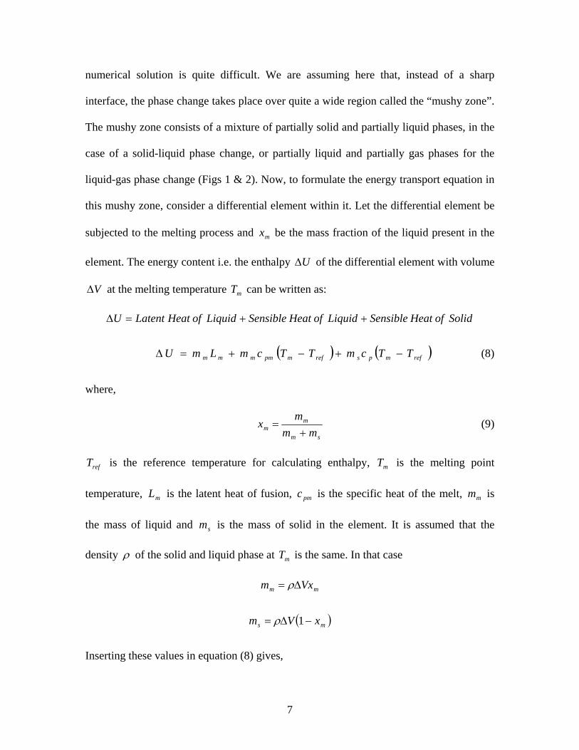
numerical solution is quite difficult. We are assuming here that, instead of a sharp

interface, the phase change takes place over quite a wide region called the “mushy zone”.

The mushy zone consists of a mixture of partially solid and partially liquid phases, in the

case of a solid-liquid phase change, or partially liquid and partially gas phases for the

liquid-gas phase change (Figs 1 & 2). Now, to formulate the energy transport equation in

this mushy zone, consider a differential element within it. Let the differential element be

subjected to the melting process and be the mass fraction of the liquid present in the

element. The energy content i.e. the enthalpy

mx

U∆ of the differential element with volume

at the melting temperature can be written as: V∆ mT

SolidofHeatSensibleLiquidofHeatSensibleLiquidofHeatLatentU ++=∆

( ) ( )refmpsrefmpmmmm TTcmTTcmLmU −+−+=∆ (8)

where,

sm

mm mm

mx

+= (9)

refT is the reference temperature for calculating enthalpy, is the melting point

temperature, is the latent heat of fusion, is the specific heat of the melt, is

the mass of liquid and is the mass of solid in the element. It is assumed that the

density

mT

mL pmc mm

sm

ρ of the solid and liquid phase at is the same. In that case mT

mm Vxm ∆= ρ

( )ms xVm −∆= 1ρ

Inserting these values in equation (8) gives,

7

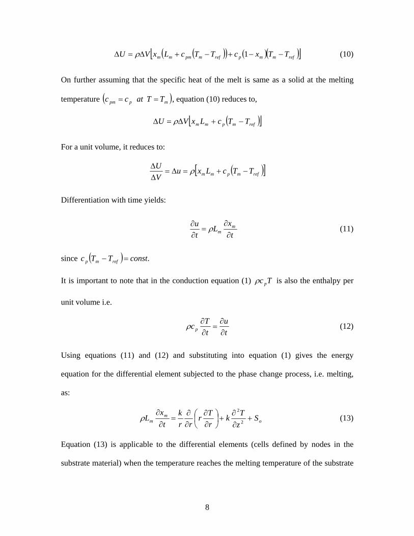
( )( ) ( )( )[ ]refmmprefmpmmm TTxcTTcLxVU −−+−+∆=∆ 1ρ (10)

On further assuming that the specific heat of the melt is same as a solid at the melting

temperature ( )mppm TTatcc == , equation (10) reduces to,

( )[ ]refmpmm TTcLxVU −+∆=∆ ρ

For a unit volume, it reduces to:

( )[ ]refmpmm TTcLxuVU

−+=∆=∆∆ ρ

Differentiation with time yields:

tx

Ltu m

m ∂∂

=∂∂ ρ (11)

since ( ) .constTTc refmp =−

It is important to note that in the conduction equation (1) Tc pρ is also the enthalpy per

unit volume i.e.

tu

tTc p ∂

∂=

∂∂ρ (12)

Using equations (11) and (12) and substituting into equation (1) gives the energy

equation for the differential element subjected to the phase change process, i.e. melting,

as:

om

m SzTk

rTr

rrk

tx

L +∂∂

+⎟⎠⎞

⎜⎝⎛

∂∂

∂∂

=∂

∂2

2

ρ (13)

Equation (13) is applicable to the differential elements (cells defined by nodes in the

substrate material) when the temperature reaches the melting temperature of the substrate

8

material and ( mTT = ) 10 ≤≤ mx , i.e. in a mushy zone. Consequently, here the

temperature of the cells with 10 ≤≤ mx is set to the melting temperature ( . When

the value of exceeds 1 ( equation (13) is no longer applicable for the

differential element under consideration because the phase change process has been

completed for that element and it is no longer in the mushy region. In this case, equation

(1) is used to determine the temperature change in the liquid phase i.e. the liquid heating

initiates and continues until the temperature reaches the boiling temperature of the

substrate material. It is important to note that inside the mushy region terms like

)

)

mTT =

mx 1>mx

rT

∂∂ and

zT

∂∂ are zero because the temperature is constant. However, equation (13) is valid at the

mushy zone/solid and mushy zone/liquid interfaces where these terms are not zero in

general.

In the case of the temperature reaching the boiling temperature, the mushy zone

consideration needs to be implemented again. In this case, equation (13) can be modified

for a differential element, which is subjected to the boiling, i.e.:

ob

b SzTk

rTr

rrk

tx

L +∂∂

+⎟⎠⎞

⎜⎝⎛

∂∂

∂∂

=∂

∂2

2

ρ (14)

Here is the latent heat of boiling or evaporation and is the mass fraction of the gas

or vapour present in the boiling differential element. The material starts ablating from the

surface elements subjected to boiling. In that case, an appropriate boundary condition is

needed at the boiling surface region. Since the boiling process occurs at a constant

bL bx

9

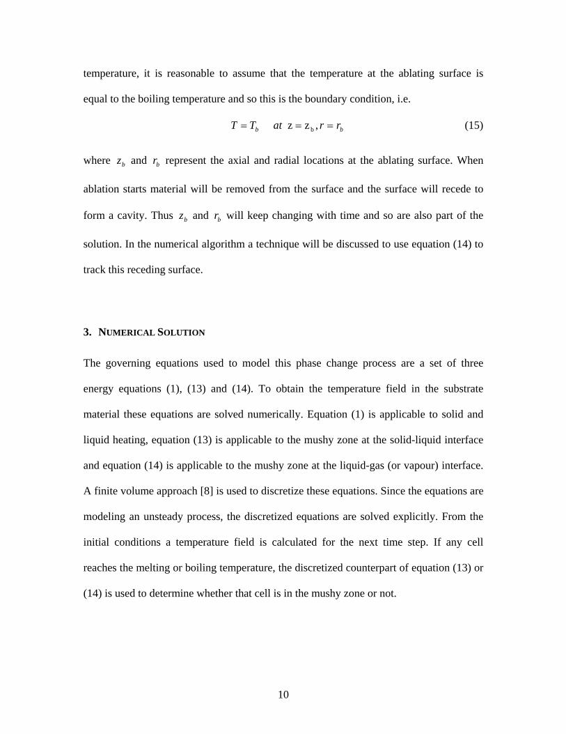
temperature, it is reasonable to assume that the temperature at the ablating surface is

equal to the boiling temperature and so this is the boundary condition, i.e.

bb rratTT === ,zz b (15)

where and represent the axial and radial locations at the ablating surface. When

ablation starts material will be removed from the surface and the surface will recede to

form a cavity. Thus and will keep changing with time and so are also part of the

solution. In the numerical algorithm a technique will be discussed to use equation (14) to

track this receding surface.

bz br

bz br

3. NUMERICAL SOLUTION

The governing equations used to model this phase change process are a set of three

energy equations (1), (13) and (14). To obtain the temperature field in the substrate

material these equations are solved numerically. Equation (1) is applicable to solid and

liquid heating, equation (13) is applicable to the mushy zone at the solid-liquid interface

and equation (14) is applicable to the mushy zone at the liquid-gas (or vapour) interface.

A finite volume approach [8] is used to discretize these equations. Since the equations are

modeling an unsteady process, the discretized equations are solved explicitly. From the

initial conditions a temperature field is calculated for the next time step. If any cell

reaches the melting or boiling temperature, the discretized counterpart of equation (13) or

(14) is used to determine whether that cell is in the mushy zone or not.

10

If, for any cell, equation (13) gives 10 ≤≤ mx , the cell is lying in the solid-liquid mushy

zone, and . Similarly, if equation (14) gives mTT = 10 ≤≤ bx , the cell is lying in the

liquid-gas mushy zone, and . bTT =

As shown in Fig 1, equation (13) will also be applicable at some points on the

boundaries. For those cases the same boundary conditions are applicable as for equation

(1). For equation (14) the boundary condition is defined in equation (15). As mentioned

earlier, equation (14) is also used to track the receding surface. Fig 1 shows that, for this

particular problem, equation (14) is applicable only on the cells near the surface. If, for

any cell, , i.e. in that particular cell all the liquid has been changed to gas and

escaped from the surface, that cell will no longer be part of the domain and the

boundaries have to be shifted to the adjacent cells in the zone.

1=bx

Since all these calculations are being performed in an explicit manner, stability analysis

[8] shows that;

12222 ≤∆⎟

⎟⎠

⎞⎜⎜⎝

⎛

∆+

∆t

zck

rck

pp ρρ (16)

Where r∆ and are the grid size in radial and axial direction respectively. The

computational domain is divided into a grid and a grid independence test was performed

for different grid sizes and distribution, resulting in a non-uniform grid with

z∆

200200×

grid points. In this set-up (Fig 3) a finer grid is used near the surface and near the axis of

symmetry, the regions where most of the energy is concentrated. The grid becomes

11

coarser as it moves towards the bulk of the substrate material. The time increment, based

on stability criteria (16), using the finest grid is calculated as seconds. A

computer program was developed to implement this scheme for calculating the

temperature field and hole geometry.

13108 −×

4. RESULTS AND DISCUSSION

Using the numerical scheme described in the previous section, the laser heating and

subsequent phase change is simulated for a step input pulse. Here steel is considered as

the substrate material and its properties are given in Table 1, whilst the laser beam

properties are given in Table 2.

Fig 4 shows the temperature variation on the surface at the beam spot centre with time.

The temperature starts to increase with heating, but at time nst 136.0= it stops

increasing. At this particular time the corresponding temperature is which shows that

the melting process has started. Once melting has been completed, the liquid heating

takes over and the temperature starts to increase again. This temperature variation is

shown to continue up to the time

mT

nst 3.0= . After this, boiling commences, material starts

to eject from the surface and the surface starts to recede towards the bulk of the substrate.

Temperature variations along the surface (Fig 5) and along the axial direction (Fig 6)

show the heating pattern during the drilling process. In Figure 5 the curves do not start

from but, rather, at some distance from the symmetry axis. Since material starts to 0=r

12

eject from the surface in the very early stages of heating, by nst 2= there is a large crater

on the surface. As the heating proceeds, with time the size of the crater on the surface

increases and this pushes the temperature curves farther away from the symmetry axis.

However, the distance between the curves decreases which shows that expansion of the

crater is slowing down. In this case, the beam has a Gaussian intensity distribution and

beyond the point where the beam intensity is less than ( )e1 times the peak intensity (Fig

3) there is not enough energy available to ablate the material from the surface. This limit

defines the radial dimension of the drilled hole. One important feature of short pulse

heating is the high temperature gradient. In the radial direction the temperature changes

from to almost room temperature within a distance of only , giving a

temperature gradient of the order of

Co 3000 m4102 −×

mC 10 o7 . There are two distinct regions on the

temperature curves. The region above shows the liquid heating, whilst the lower

part is the solid heating. The two regions are separated by a bump on the curve around

that corresponds to the mushy zone at the solid-liquid interface. The

temperature variation along the symmetry axis shows an almost similar behaviour to its

radial counterpart. One obvious difference is the way in which the curves shift away from

the surface. Because of the material removal, the surface recedes towards the bulk of the

material. Here, unlike the radial variation, the distance between the curves does not

change which shows that near the symmetry axis the material removal rate and surface

recession is uniform and does not slow down with time. Unlike the radial direction, when

the depth of the cavity increases in the axial direction, the newly exposed material

receives the same amount of energy as the old surface, which causes the same removal

rate to occur. Another difference between the radial and axial temperature variations is

Co 1800

Co 1800

13

the temperature gradient. In the axial direction the temperature gradient is even higher, of

the order of . 910

In short pulse laser heating a high amount of localized energy is deposited in the substrate

material. In the early heating period, a high-energy deposition rate results in a sharp

temperature rise in the vicinity of the surface and the bulk of the substrate remains at a

relatively lower temperature. Because of such a short duration, the energy cannot diffuse

in the bulk of the material. As the heating proceeds, it would be expected that diffusion

should take over. However, once the surface temperature reaches boiling point, material

starts to eject from the surface and so at each time step a new surface is exposed to the

laser beam. This process holds the diffusional effects in check, whilst the phase change

and material removal consume the better part of the energy deposited.

The curves in Fig 7 show the surface of the drilled hole. These curves represent surface

of revolution. The cavity surface development is in accord with the discussion for the

temperature variation in the substrate. In the early heating period, the cavity development

in the radial direction is fast but it slows down as it reaches the ( )e1 point of the beam

intensity (Fig 3). On the other hand, in the axial direction the cavity keeps extending.

This results in the walls of the drilled hole becoming steeper, whilst near the base of the

hole the surface acquires a sharper curvature.

14

Figs 8 and 9 show the temperature contours inside the substrate material at 4 and 8

nanoseconds, respectively. The energy deposition rate is 212 107 m

W× , with a pulse

length of 8 ns. This typical contour shape arises from the surface ablation and the cavity

formation in the substrate material. As described previously, the cavity does not expand

much in the radial direction but the change in the axial direction is very prominent. The

contour plots show that although these contours are moving as the surface ablation is

progressing, they do not really penetrate into the substrate material. This indicates that

there is insufficient diffusion taking place such that the heat does not conduct toward the

bulk of the substrate. In a very thin region near the surface, energy is absorbed and this

immediately raises the temperature. Before any heat diffusion can take place, the

temperature reaches the boiling point and material starts to eject from the surface. Thus,

most of the energy deposited in short pulse heating is used in cavity formation rather than

in heating of the bulk of the substrate. The contours with temperatures above

represent the very thin liquid phase layer developed in the cavity.

Co 1800

Unlike conventional drilling processes, laser drilling relies on phase change and for this

purpose the substrate is brought to temperatures far beyond the re-crystallization

temperature. Laser drilling can produce a very large heat affected zone where the material

properties may differ from the bulk of the substrate.

To see the effect of the laser parameters, namely the beam intensity and pulse length, on

the development of the heat affected zone, simulations are performed for different pulse

15

lengths and beam intensities. Since a wide range of laser beam intensity and energies are

available, arbitrary values may be chosen. In this study these parameters are adjusted

such that almost the same depth of drilled hole is achieved as for the 8 ns pulse. Figs 10,

11, 12 show temperature contours for beams with pulse lengths of 6, 4 and 2 ns and beam

intensities of , and 12103.9 × 121014 × 212 1028 m

W× , respectively. It appears from these

contours that with decreasing pulse length and increasing beam intensity, the depth of the

heat-affected zone reduces considerably. Fig 13 shows the temperature variation along

the axial direction for various beam intensities, confirming the fact that the temperature

decreases at a much faster rate along the axial direction with increasing intensity, as was

also observed from the temperature contours. The temperature at the surface of the cavity

is in the vicinity of the boiling temperature for all the beam intensities studied. Moving a

short distance away towards the bulk of the material the temperature difference at any

given point for different beam intensities could be significant, e.g. at the depth of

temperatures for m61018.1 −× 2121028 m

W× and 212107 m

W× beams are and

, respectively. This observation confirms the energy interaction picture

described previously. When the energy deposition rate increases, the rate of temperature

rise in the surface vicinity increases as well. With negligible heat diffusion toward the

bulk of the material, the surface starts evaporating. Fig 14 shows the variation of the

temperature gradient along the axial direction for various beam intensities. Since the

temperature at the surface is the boiling temperature of the material and it decreases

rapidly as we move away from the surface, it results in very large temperature gradients.

Here, it is obvious that with an increase in the beam intensity the peak temperature

gradient value also increases. It has been shown in previous work [9] that large

Co 1810

Co 2390

16

temperature gradients in laser heating result in very large thermal stresses in the substrate

material. But, interestingly, here the large thermal gradient generated with increasing

beam intensity is confined to the liquid phase and in the solid phase the temperature

gradients are not very much different for different beam intensities. Hence, it may be

expected that different beam intensities will generate almost identical stress fields.

It is interesting to note from Figs 8 and 9 that the pulse length has no effect on the size of

the heat-affected zone. With a longer pulse a deeper drilled hole is achieved, although the

depth of the heat-affected zone remains same. Indeed, the depth of the heat-affected zone

is more dependent on the energy deposition rate.

5. CONCLUSIONS

In this study a laser heating process with phase change is modeled. To model the phase

changes involved in the process the concept of a “mushy zone” is introduced and an

appropriate form of the energy equations is derived for the solid-liquid and liquid-gas

mushy zones. These model equations are solved numerically to obtain the temperature

field and the shape of the drilled hole. The following conclusions are derived from this

work:

1. The model described in this study captures the phase change process in laser

heating.

17

2. There is a high temperature gradient generated in the vicinity of the surface. With

a high-energy deposition rate, material ejection from the surface overcomes the

diffusion of energy to the bulk of the substrate.

3. The drilled hole expands in the axial direction at a steady rate but the expansion in

the radial direction is limited because of the radial energy distribution in the

beam.

4. The depth of the heat-affected zone in the substrate material is independent of

pulse length, whereas it can be reduced by using a larger pulse intensity.

6. REFERENCES

[1] Yilbas, B. S., Analytical solution for time unsteady laser pulse heating of semi-

infinite solid, Int. J. Mech. Sci., 39(6), 1997, 671-682.

[2] Modest, M. F. and Abakians, H., Evaporative cutting of a semi-infinite body with a

moving cw laser, Trans. ASME, J. Heat Transfer, 108, 1988, 602-607.

[3] Basu, B. and Date, A. W., Numerical study of steady state and transient laser melting

problems-I. Characteristics of flow field and heat transfer, Int. J. Heat and Mass Transfer,

33, 1990, 1149-1163.

[4] Wei, P. S. and Ho, J. Y., Energy considerations in high energy beam drilling, Int. J.

Heat and Mass Transfer, 33(10), 1990, 2207-2217.

[5] Bang, S. Y. and Modest, M. F., Multiple reflection effects on evaporative cutting

with a moving cw laser, Trans. ASME, J. Heat Transfer, 113, 1991, 663-669.

18

[6] Ganesh, R. K., Faghri, A. and Hahn, Y., A generalized thermal modeling for laser

drilling process-I. Mathematical modeling and numerical methodology, Int. J. Heat and

Mass Transfer, 40(14), 1997, 3351-3360.

[7] Ganesh, R. K., Faghri, A. and Hahn, Y., A generalized thermal modeling for laser

drilling process-II. Numerical simulation and results, Int. J. Heat and Mass Transfer,

40(14), 1997, 3361-3373.

[8] Patanker, S. V., Numerical Heat Transfer and Fluid Flow, Hemisphere Publishing

Corp., 1980.

[9] Yilbas, B.S. and Naqavi I.Z., Laser heating including the phase change process and

thermal stress generation in relation to drilling, Proc. Instn. Mech. Engrs. Part B J.

Engineering Manufacture,Vol. 217, 2003, 977-991.

19

Thermal

conductivity

( )mKWk

Specific heat

⎟⎠⎞⎜

⎝⎛

kgKJc p

Density

⎟⎠⎞⎜

⎝⎛

3 mkgρ

Latent heat of

fusion

⎟⎠⎞⎜

⎝⎛

kgJLm

52 330 7836 5104.2 ×

Latent heat of

boiling

⎟⎠⎞⎜

⎝⎛

kgJLb

Melting temperature

( )KTm

Boiling temperature

( )KTb

61026.6 × 1810 3030

Table 1: Material properties for steel.

Pulse intensity

( )2 mWIo

Absorption depth

parameter

( )m1 δ

Gaussian

parameter

( )ma

Heating period

( )ns

7, 9.3, 14 &

28 ( )1210×

61016.6 × 41006.3 −× 8, 6, 4 & 2

Table 2: Properties of the laser beam

20

Figure 1: Axisymmetric heating and surface ablation with two mushy zones.

Figure 2: Schematic view of the mushy cell.

21

Figure 3: Gaussian beam profile and numerical grid in the physical domain.

0

500

1000

1500

2000

2500

3000

3500

0.00 0.05 0.10 0.15 0.20 0.25 0.30

t (nsec)

T (o C

)

Temp.

Figure 4: Temporal variation of temperature at the beam centre with step input pulse.

22

0

500

1000

1500

2000

2500

3000

3500

0.0E+00 2.0E-04 4.0E-04 6.0E-04 8.0E-04 1.0E-03

r (m)

T (o C

)

t = 2 nsect = 4 nsect = 6 nsect = 8 nsec

Figure 5: Spatial temperature variation along the surface.

0

500

1000

1500

2000

2500

3000

3500

0.0E+00 5.0E-07 1.0E-06 1.5E-06 2.0E-06

z (m)

T (o C

)

t = 2 nsec

t = 4 nsec

t = 6 nsec

t = 8 nsec

Figure 6: Spatial temperature variation along the axial direction.

23

0.0E+00

2.0E-07

4.0E-07

6.0E-07

8.0E-07

0.0E+00 1.0E-04 2.0E-04 3.0E-04 4.0E-04

r (m)

z (m

)t = 2 nsect = 4 nsect = 6 nsect = 8 nsec

Figure 7: Development of the drilled hole geometry.

24

1 8 9 . 4

1 8 9 .4

1 8 9 . 4

5 6 8 . 1

5 6 8 .1

9 4 6 .9

9 4 6 .9

1 3 2 5 .6

1 32 5

.6

1 7 0 4 .4

1 7 0 4 . 4

2 0 8 3 .1

2 4 6 1 .9

2 4 6 1 .9

2 8 4 0 .6

2 8 4 0 .6

r ( m )0 0 . 0 0 0 2 0 . 0 0 0 4 0 . 0 0 0 6 0 . 0 0 0 8

0 .0 0 E + 0 0

2 . 5 0 E - 0 7

5 . 0 0 E - 0 7

7 . 5 0 E - 0 7

1 . 0 0 E - 0 6

1 . 2 5 E - 0 6

1 . 5 0 E - 0 6

1 . 7 5 E - 0 6

2 . 0 0 E - 0 6

z(m

)

Figure 8: Temperature contours in the substrate at 4 ns with pulse intensity of

212107 m

W× .

1 8 9 .4

1 8 9 .4

1 8 9 .4

5 6 8 .1

5 6 8 .1

5 68 .

1

9 4 6 . 9

9 4 6 .9

9 46 .

9

1 3 2 5 .6

1 3 2 5 . 6

1 7 0 4 . 4

1 7 0 4 .4

1 7 0 4 . 4

2 0 8 3 .1

2 0 8 3 .1

2 4 6 1 . 9

2 4 6 1 .9

246 1

.9

2 8 4 0 .6

2 8 4 0 . 6

r ( m )0 0 . 0 0 0 2 0 . 0 0 0 4 0 . 0 0 0 6 0 . 0 0 0 8

0 . 0 0 E + 0 0

2 .5 0 E - 0 7

5 .0 0 E - 0 7

7 .5 0 E - 0 7

1 .0 0 E - 0 6

1 .2 5 E - 0 6

1 .5 0 E - 0 6

1 .7 5 E - 0 6

2 .0 0 E - 0 6

z(m

)

Figure 9: Temperature contours in the substrate at 8 ns with pulse intensity of

212107 m

W× .

25

1 8 9 .4

1 8 9 . 4

1 89 .

4

5 6 8 .1

5 6 8 . 1

9 4 6 . 9

9 4 6 .9

1 3 2 5 . 6

1 3 2 5 .6

1 7 0 4 .4

1 7 0 4 .4

1 70 4

.4

2 4 6 1 .9

2 0 8 3 . 1

2 4 6 1 .9

2 27 2

. 5

2 8 4 0 .6

2 8 4 0 . 6

r ( m )0 0 . 0 0 0 2 0 . 0 0 0 4 0 . 0 0 0 6 0 . 0 0 0 8

0 . 0 0 E + 0 0

2 . 5 0 E - 0 7

5 . 0 0 E - 0 7

7 . 5 0 E - 0 7

1 . 0 0 E - 0 6

1 . 2 5 E - 0 6

1 . 5 0 E - 0 6

1 . 7 5 E - 0 6

2 . 0 0 E - 0 6

z(m

)

Figure 10:Temperature contours in the substrate at 6 ns with pulse intensity of

212103.9 m

W× .

1 8 9 . 4

1 8 9 . 4

1 89 .

4

5 6 8 .1

5 6 8 . 1

9 4 6 .9

9 4 6 . 9

1 3 2 5 .6

1 32 5

.6

1 7 0 4 .4

1 7 0 4 .4

2 0 8 3 . 1

2 08 3

. 1

2 6 5 1 . 3

2 4 6 1 .9

2 8 4 0 .6

2 8 4 0 .6

r ( m )0 0 .0 0 0 2 0 . 0 0 0 4 0 . 0 0 0 6 0 . 0 0 0 8

0 . 0 0 E + 0 0

2 .5 0 E - 0 7

5 .0 0 E - 0 7

7 .5 0 E - 0 7

1 .0 0 E - 0 6

1 .2 5 E - 0 6

1 .5 0 E - 0 6

1 .7 5 E - 0 6

2 .0 0 E - 0 6

z(m

)

Figure 11: Temperature contours in the substrate at 4 ns with pulse intensity of

2121014 m

W× .

26

1 8 9 .4

1 8 9 .4

5 6 8 . 1

5 6 8 .1

9 4 6 .9

9 4 6 .9

1 3 2 5 .6

1 3 2 5 .6

1 7 0 4 .4

1 7 0 4 .4

1 8 9 3 .8

2 08 3

.1

2 4 6 1 .9

2 4 6 1 .9

2 8 4 0 .6

2 8 4 0 .6

r ( m )0 0 . 0 0 0 2 0 . 0 0 0 4 0 . 0 0 0 6 0 . 0 0 0 8

0 . 0 0 E + 0 0

2 . 5 0 E - 0 7

5 . 0 0 E - 0 7

7 . 5 0 E - 0 7

1 . 0 0 E - 0 6

1 . 2 5 E - 0 6

1 . 5 0 E - 0 6

1 . 7 5 E - 0 6

2 . 0 0 E - 0 6

z(m

)

Figure 12: Temperature contours in the substrate at 2 ns with the pulse intensity of

2121028 m

W× .

27

0

500

1000

1500

2000

2500

3000

3500

1.0E-06 1.2E-06 1.4E-06 1.6E-06 1.8E-06 2.0E-06z (m)

T (o C

)7x10^12 W/m^29.3x10^12 W/m^214x10^12 W/m^228x10^12 W/m^2

Figure 13: Spatial temperature variation along axial direction for different beam intensities.

-2.0E+10

-1.6E+10

-1.2E+10

-8.0E+09

-4.0E+09

0.0E+00

4.0E+09

1.0E-06 1.2E-06 1.4E-06 1.6E-06 1.8E-06 2.0E-06

z (m)

dT/d

z

7x10^12 W/m^29.3x10^12 W/m^214x10^12 W/m^228x10^12 W/m^2

Figure 14: Spatial temperature gradient variation along axial direction for different beam intensities.

28