Engineering Structures 33 (2011) 2850–2860

Contents lists available at ScienceDirect

Engineering Structures

journal homepage: www.elsevier.com/locate/engstruct

A numerical procedure for simulating the multi-support seismic response ofsubmerged floating tunnels anchored by cablesLuca Martinelli a,∗, Gianluca Barbella a, Anna Feriani ba Department of Structural Engineering, Politecnico di Milano, Milano, Italyb Department of Civil Engineering, Architecture, Land and Environment, University of Brescia, Brescia, Italy

a r t i c l e i n f o

Article history:Received 9 April 2010Received in revised form26 May 2011Accepted 1 June 2011Available online 5 July 2011

Keywords:Multiple-support seismic excitationNon-linear dynamicsGeometrical effects

a b s t r a c t

The modeling and seismic analysis of submerged floating tunnels moored by cables is addressed withparticular attention to spatial variability of the excitation. Dissipation modeling issues and cables dis-cretization are also discussed.

A uniformly modulated random process, whose spatial variability is governed by a single coherencyfunction, is deemed adequate to model the multi-support seismic input for a given structure of largedimension undergoing limited plastic deformation, as the one considered here. A novel method to obtainresponse spectrum compatible accelerograms is proposed, based on the explicit expression of themedianpseudo-acceleration response spectrum induced by the adopted power density function (PSD). Thisexpression is used to identify the parameters of the PSD function that minimize the difference with theelastic response spectrum prescribed by EN 1998; the minimization process is discussed and parametersfor the PSD spectra are obtained. Samples of the free-field motion are then generated using a proved andtheoretically sound approach and reach a satisfactory agreement with the prescribed response spectra.

To model the cables, a 3 node isoparametric cable element is enriched by including hydrodynamicloading, within a numerical procedure for the dynamic time domain step-by-step analysis of non-lineardiscretized systems.

An example of application is shown that makes reference to the bed profile of Qiandao Lake (People’sRepublic of China), where a plan exists to build the first SFT prototype.

© 2011 Elsevier Ltd. All rights reserved.

1. Introduction

Submerged Floating Tunnels (SFTs) can be a valid alternative tolong-span bridges for crossing sea straits, fjords or inland waters.SFTs basically consist of a cylindrical tunnel floating at a certaindepth below the water surface, moored by an anchoring systemthat relies on slender elements: either cables or bars. Since SFTscan be set at a specific depth below the water table, they do notneed long and/or steep approaching roadways that are, instead,necessary for conventional underground tunnels or traditionalimmersed tunnels resting on the seabed, and can be thus moreeconomic.

The dynamic response of SFTs to several environmental actionsis of interest, among which are waves, current and consequentlyvortex induced vibrations, and earthquakes. Finally, these inducenot only inertial loads but also hydrodynamic ones. Non-linear

∗ Corresponding author. Tel.: +39 0 2 2399 4247; fax: +39 0 2 2399 4220.E-mail addresses: luca.martinelli@polimi.it, martinel@stru.polimi.it

(L. Martinelli), barbella@stru.polimi.it (G. Barbella), anna.feriani@ing.unibs.it(A. Feriani).

0141-0296/$ – see front matter© 2011 Elsevier Ltd. All rights reserved.doi:10.1016/j.engstruct.2011.06.009

dynamic analyses are required to correctly model both the hydro-dynamic loads and the geometrically non-linear behavior of theanchoring system, whose stiffness and resistance depend also onthe SFT buoyancy effects.Whenever the SFT length requires it, seis-mic analyses must account for the spatial variability of the groundmotion.

The work presented herein is focused, first, on accounting forthe above-mentioned ground motion spatial variability while sat-isfying a code prescribed response spectrum and, second, on somemodeling aspects of an SFT moored by cables.

As for the first goal, in Sections 2 and 3we propose a generationprocedure of the seismic input that leads to the results harmonizedwith EN 1998 [1] prescriptions. When a multi-support analysis isrequired, due to the lack of data, one has often to resort to artificialtime histories. In effect, as detailed in [2], EN 1998 requires morejustifications in order to use recorded accelerograms, or simulatedaccelerograms generated through a seismological model, with re-spect to the use of artificial time histories. The problem of gen-erating acceleration time histories representative of earthquakemotion at different stations is probably one among those that at-tracted the largest interest by researchers; a recent overview of theconcepts involved can be found in the over 130 references listedin [3].

L. Martinelli et al. / Engineering Structures 33 (2011) 2850–2860 2851

Engineering models usually relate the seismic motion to arealization of a stochastic process and consider in a probabilisticway the effects of the propagation path on the differences ofthe motion at different points. Seismological models, which arenormally more involved, introduce also a description of the sourceof the earthquake and of its propagation path.

A classical engineering model for generating acceleration timehistories resorts to the spectral representation of the stochasticprocess. According to this model, acceleration time histories canbe easily generated starting from the power spectrum densityfunction (PSD) of the stochastic process; a problem arises,however, when it is required that the acceleration time historiescomply to a code specified response spectrum. In this case, iterativemethods, like the ones in [4–6], are required to derive a suitablePSD that will give rise to time histories with response spectrasatisfying, on average, the one specified by the code.

As part of this work a procedure has been developed togenerate acceleration time histories that are compatible with theEN 1998 pseudo-acceleration elastic response spectrum (Se,EN1998hereafter), while relying on a proven procedure to represent themotion spatial variability. The method by Monti et al. [7] isadopted here to generate acceleration time histories which havethe same PSD function at all stations while the cross-PSDs satisfya single coherency function which models the spatial correlation.As a distinguishing aspect, however, in this work the parametersof the PSD function are carefully chosen in order to minimizethe difference between the median pseudo-acceleration responsespectrum (RSa hereafter) of the generated time histories andSe,EN1998. The minimization process is based on the knowledge ofthe explicit equation of RSa. With reference to the Kanai–TajimiPSD asmodified by Clough andPenzien [8] (ModifiedKanai–Tajimi,MKT, hereafter), this is given for the first time in this work, to theauthors’ knowledge.

As to the second purpose of the work, related to structuralmodeling, this requires enhancement of the numerical proceduredeveloped by the research group [9–12], which performs thestep-by-step dynamic analysis of discretized non-linear structuralsystems under arbitrary external loading, allowing for multiple-support seismic excitation.

The procedure is here applied to SFTs and is enhanced byenriching the mooring cables model, as described in Section 4. Thecable model is based on a Lagrangian three-node isoparametriccable element, formulated in the small-strain large-displacementhypothesis [13], further developed and coded in [10]. In this work,in order to model submerged cables, the implementation of theelement has been extended including the added mass matrix andthe non-linear hydrodynamic loads, determined according to theMorison approach.

Structural damping is modeled by merging two previous pro-cedures, obtaining a banded global equivalent viscous matrix, thatthanks to an iteration process represents accurately equivalentmodal damping factors, as detailed in Section 6.

In this work an example of application is shown, that makesreference to the bed profile of Qiandao Lake (People’s Republic ofChina), where a plan exists to build the first SFT prototype, andwhere the EN 1998 response spectrum was assumed as an initialdesign requirement.

2. Description of the seismic ground motion

A spatial description of themotion can be obtained by assumingthat the motion induced by the earthquake at each station i is arealization of a common stochastic process.

The seismic motion is by its own nature non-stationary. Thisnon-stationarity is related both to the amplitude of the motion, aswell as to its frequency content, which both change in time.

A possible way to characterize the time-varying nature offrequency content in seismic action is by representing theacceleration a(t) as a realization of a so-called evolutionary randomprocess [14]. The importance of the non-stationary frequencycharacteristic of the seismic ground motion for an elastic–plasticstructure is shown e.g. in the work by Wang et al. [15]; however,considering that SFTs are normally designed to behave elasticallyunder all the design scenarios, and that the one at the base of thisstudy has a stiffening behavior due to cable stretching, the issueof non-stationarity due to evolution of the frequency content is inthis case secondary.

It thus becomespossible, as done in thiswork, tomodel the non-stationary process representing the acceleration by the simpleruniformly modulated random process, which has the form a(t) =

f (t)x(t), where f (t) is a deterministic envelope function with amaximum value of 1 and x(t) is a stationary process. Such anassumption is equivalent to considering a random process withnon-stationary intensity but time invariant frequency content.

The effect of the non-stationarity of the amplitude, which is de-scribed by the function f (t), has been extensively studied in thepast [16], where the authors conclude that no simple and practicalway exists to define physically realistic envelopes. Since envelopefunctions commonly used cannot be considered unique and real-istic, only the highest response amplitudes can be regarded as re-liable. These same highest amplitudes can however be computedin a simpler way from a stationary process of suitable duration s0,which is defined in [17] as a function of the natural period of theoscillator and of its damping ratio.

The deterministic envelope f (t) here adopted, proposed byAmin and Ang [18], is:

f = (t/t0)2 0 < t < t0f = 1.0 t0 < t < tnf = e−0.155(t−tn) tn < t.

(1)

The contribution of the differentwave types to the time history canbe considered recalling that the difference tn–t0 is the significantduration of the accelerogram and is the interval within whichthe S-waves are predominant. It will be assumed as the durations0 of the stationary part hereafter. As discussed in [2], s0 can berelated to the Arias intensity and to the Peak Ground Acceleration(PGA) estimated at the site. The real duration associated withthe envelope function of (1) is larger than tn–t0; however thechoice made will not lead to large errors in matching the targetresponse spectrum, as it will be shown later. In the envelopefunction t0 models the time lag between the P- and S-waves, soit can be chosen according to the distance between the site and thehypocenter.

In order to define x(t), a possible approach to the problem isby assuming that the motion induced by the earthquake at eachstation i is a realization of a common stochastic process. Thisunderlying process can be characterized by its PSD Sii, while thestatistical differences between the motion at two stations i and jare described by the coherency function γij(ω) [19]:

γij(ω) =Sij (ω)

√Sii (ω)

Sjj (ω)

. (2)

At the circular frequency ω, this function relates the cross-powerspectral density function Sij(ω), between stations i and j, with theauto-spectra Sii and Sjj.

The coherency is a complex function; its modulus, |γ |, termed‘‘lagged coherency’’, represents a measure of the statisticaldifferences of the ground motion between stations i and j, whileits phase represents its systematic differences [19]. Experimentalevidence points out that the latter increases with the distance ξL

2852 L. Martinelli et al. / Engineering Structures 33 (2011) 2850–2860

between the stations and with the circular frequency ω. Theseaspects are reflected by the coherency functions proposed inliterature [20–25], which also retain the form, and the physicalmeaning, of the amplitude–phase expression:

γij(ξL, ω) = e−α(ω,ξL)aeiβ(ω,ξL)

b(3)

where local effects are disregarded and the exponents a and bweigh differently the two terms.

While the generation method of artificial time histories wepropose, described in the next section, can be extended to otherPSD and coherency functions, in the present work the Luco andWong [23] coherency function is assumed, as in [7], disregardinglocal effects :

γ (ξ, ω) = e−

αωξvs

2ei

ωξLvapp . (4)

In (4) the modulus decays exponentially with the horizontaldistance ξ between the stations, with the circular frequencyω, andinverselywith themechanical properties of the ground, condensedin the ratio vs/α where vs is the shear waves velocity. The phasedepends linearly on ω, on the relative distance ξL and on theinverse of the apparent velocity at the surface, vapp, of the seismicperturbation. In the generation process, the phase given by theimaginary part in (4) leads to a time delay only, due to the finitewave propagation velocity.

The direct PSD Sii of the underlying process, here adopted, isthe MKT PSD [8], which can be viewed as the effect of a filter,representing the soil, on a white noise process which represents,in turn, the motion of the bedrock:

Sg (ω) = S0SCP (ω)

= S0ω4

1 + 4ξ 21 ω2

1ω2

ω21 − ω2

2+ 4ξ 2

1 ω21ω

2

ω4ω2

2 − ω22

+ 4ξ 22 ω2

2ω2

(5)

where S0 is the intensity of the white noise process in input tothe ground (bedrock motion), ω1 and ξ1 are the parameters ofthe Kanai–Tajimi filter representing the soil natural frequency anddamping ratio, respectively, while ω2 and ξ2 are the parameters ofan additional high-pass filter introduced by Clough and Penzien toguarantee that displacements possess finite power.

3. Generation of the seismic ground motion

In this work, a novel way is followed to generate acceleration(and displacement) time histories that, on one side, are compatiblewith a prescribed pseudo-acceleration elastic response spectrum(Se,EN1998 herein) while, on the other, reflect the spatial variabilityrequired for large structures.

Methods like that in [25] by Hao et al. and in [26–28] byShinozuka allow for the generation of realizations of accelerationtime histories possessing predefined direct (Sii) and cross-spectralpower density functions (Sij) between different points in space.Here, the method by Monti et al. described in [7], which relies onthe proven spectral representation method by Shinozuka [26], isadopted to generate acceleration time histories which satisfy thesame PSD function at all stations and have cross-PSD functionsdepending on one coherency function only. In the present work,however, the parameters of this PSD are carefully chosen in orderto minimize the difference between RSa and Se,EN1998.

The minimization procedure is based on the knowledge of theequation expressing the RSa consequent to ground accelerationscomplying with the adopted PSD. With reference to the MKT PSD,this equation is given for the first time, to the authors’ knowledge.In this way, the generated acceleration time histories almostsatisfy, on average, Se,EN1998, while retaining the utilization of theproven generation method [11] described in Monti [7].

3.1. Response spectrum for an SDOF excited by a given PSD

We develop the expression of the response spectrum for aSingle Degree of Freedom (SDOF) elastic oscillator recalling that,according to Vanmarcke [29], the expected (median) value ymax,over the time period s0, of the peak (extreme) value of a stationaryprocess y, having PSD defined by the function Sy(ω), can becomputed, introducing the peak factor p, as:

ymax = pvar [y] (6)

where:

ymax is the value of the extreme response which has50% probability to be exceeded,

p =

2 log

2.88Ωs02π

is the peak factor and ‘‘Log’’

denotes the natural logarithm (7)s0 is the observation interval (here strong motion duration),

Ω =

var [y]var [y]

is the expected circular frequency

for the response during s0, (8)

var [y] =

∫+∞

−∞

ω2Sy (ω) dω is the variance of the

derived process, (9)

var [y] =

∫+∞

−∞

Sy (ω) dω is the variance of the process. (10)

Then, Sy(ω) is selected as the PSD, Sd(ω), of the relative displace-ment d for a SDOF elastic oscillator excited by an accelerationwhich satisfies a given PSD, Sg (ω), that is:

Sy (ω) = Sd (ω) = Sg (ω) |Hd|2 (11)

whereHd is the complex response function for the SDOF elastic os-cillator of natural frequency ωs and damping ratio ξs:

Hd =−1

ω2s − ω2 + i2ξsωsω

. (12)

Eqs. (6)–(10) can be used to compute the displacement responsespectrum RSd corresponding to Sd (ω). In general this responsespectrum will differ from Se,EN1998 and, to approximate it, a mini-mization process over the ground acceleration PSDparameterswillbe required. Owing to the fact that the median response spectrumdefined by (6) has to be recomputed several times during the min-imization process, a different approach from that of numericallyevaluating the integrals in (9) and (10) has to be sought. Here, withreference to the MKT PSD, the analytic expression for RSa is com-puted, and the explicit equation is used in minimizing the differ-ence with Se,EN1998. Hence a faster multidimensional minimizationprocess is carried out and knowledge of the equation allows to eas-ily match other prescribed response spectra if compliance with adifferent code is required.

3.2. Analytical computation of the response spectrum related to theClough and Penzien PSD

If the MKT PSD (5) is adopted for ground acceleration, theconsequent PSD, Sd(ω), of the relative displacement is a rationalfunction as well as the output of a stable linear dynamic system;this allows for computing the integrals in (9) and (10) resorting tocontour integration in the complex plane, so that the variance forthe relative displacement d of the SDOF can be computed as [2]:

L. Martinelli et al. / Engineering Structures 33 (2011) 2850–2860 2853

var[d] =

∫+∞

−∞

Sd (ω) dω = πS0ω21A

B(13)

where A and B are detailed in Appendix. Having defined C as inAppendix, the variance of the velocity results:

var[d] =

∫∞

−∞

Sd(ω)dω = πS0ω21C

B. (14)

Consequently, the Vanmarcke peak factor p (7) can be analyticallycomputed, and from this the response spectrum RSd for the relativedisplacement d (6):

RSd(ω1, ζ1, ω2, ζ2, ωs, ζs, S0, s0) = pvar[d]. (15)

Having computed RSd, the analytical expression of median re-sponse spectrum RSa = ω2

s RSd is easily obtainable:RSa(ω1, ζ1, ω2, ζ2, ωs, ζs, S0, s0)

= ω2s

2 log

75π

s0

C

A

var[d]. (16)

3.3. Minimization process to determine the parameters of the MKTPSD for compatibility with Se,EN1998

The sets of parameters ω1, ξ1, ω2, ξ2, S0, s0 for the explicitexpression of RSa, obtained in the previous subsection can beidentified byminimizing the errorwith the EN 1998 horizontal andvertical elastic design response spectra, Se and Sve respectively. Tothis aim, the following error function G is defined:

G(p) =

∫ Tu

Ti(RSa (Ts, ζs, p) − Se.EN1998 (Ts, ζs))2 dT (17)

where Ts = 2π/ωs and p = [ω1, ξ1, ω2, ξ2, S0, s0] is thevector listing the parameters which define the MKT PSD and theunderlying stationary process, while Se.EN1998 represents either Seor Sve.

Minimization of the non-linear function G was performed inthe MATLAB environment using the unconstrained minimizationprocess available through the fminsearch function. This usesthe simplex search method of Lagarias et al. [30] and solvesan unconstrained non-linear optimization problem finding theminimum of a scalar function of several variables, starting at aninitial estimate. The numerical algorithm fminsearch employs is adirect search method and does not require the function G to becontinuously differentiable. Therefore, the implementation doesnot require the knowledge of the gradient and of the Hessian ofthe function G.

3.4. Parameters of the MKT PSD for compatibility with the EN 1998response spectrum

In thiswork, the parameters of the PSDhave been chosen so thatRSa complies with the ‘‘type 1’’ EN 1998 elastic design spectra fora type ‘‘C’’ soil. A parameters choice for the other soil types and forthe ‘‘type 2’’ spectra are presented in [2] where sensitivity to initialvalues is also discussed, in order to evaluate the minimizationprocess.

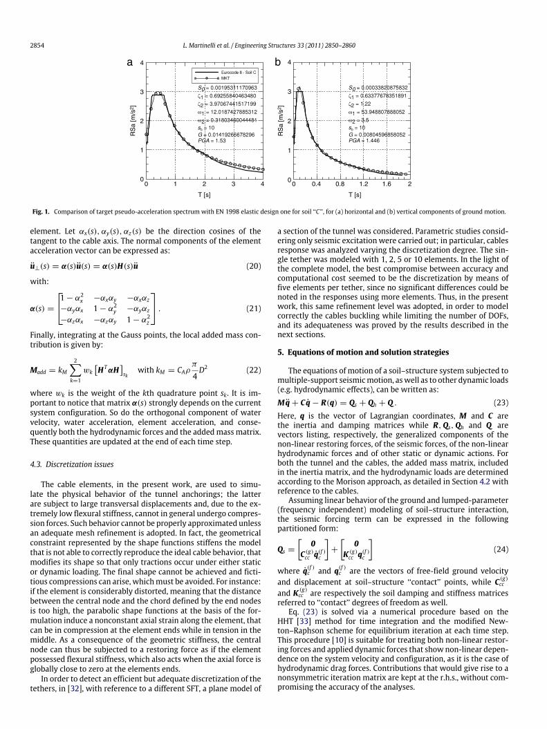
Two sets of parameters, for the explicit expression of RSaobtained in the previous subsection, have been identified byminimizing the error with the elastic design spectra Se and Sverespectively. A damping ratio ξs = 0.05 was considered inthe fittings, since the EN 1998 spectra refer to such damping.Parameter s0 coincides with tmax = tn − t0 = 10 s. In theminimization process, the period range from Ti = 0.001 s toTu = 2 s was considered. The identified values of ω1, ζ1, ω2, ζ2, S0are listed in Table 1. The visual comparison with the target spectrais depicted in Fig. 1a and b.

Table 1Values of the parameters that minimize the error with the ‘‘type 1’’ EN 1998horizontal (Se) and vertical (Sve) elastic design response spectrum in the periodsrange 0.001–2 s for type ‘‘C ’’soil.

ω1 [rad s−1] ζ1 ω2 [rad s−1] ζ2 S0 [m2 s−4 Hz−1]

Se 12.02 0.6926 0.3180 3.971 0.001953Sve 53.95 0.6338 3.50 1.22 3.382 × 10−4

4. The cable element

4.1. Formulation hypotheses

In this work three-node isoparametric cable elements are usedto model the tunnel anchorings. The adopted cable element,implemented in the FE code used for the analyses, follows theLagrangian formulation under the hypothesis of small strains andlarge displacements. It is derived from the explicit formulationproposed in [13] with reference to the static case, extended to thedynamic case and coded in [10] to fully consider the non-lineareffects of the motion of the structure on aerodynamic interactionforces. The single element matrices and internal forces vectors aredirectly computed with respect to the global coordinates system,so that no transformation is needed in the assembling procedure. Inthe numerical implementation of the element, the elastic stiffnessterms have been evaluated in closed form, while two points Gaussquadrature has been used for the geometric stiffness and forinternal forces.

The element mass matrix coefficients have been computed inclosed form, as well.

4.2. Hydrodynamic loading

The cable element has been enriched herein by introducinghydrodynamic forces according to the Morison–Chakrabarti [31]approach, which is well justified, on geometrical grounds, for theanchor cables; the relative velocity model has been adopted andtangential forces have been neglected. Accordingly, the wave forceper unit length acting on a moving cylinder is a function of thecomponents of kinematic vectors, that is relative velocity (w − u),water acceleration w, and element acceleration u, normal to theelement axis, i.e.:

f =12CDρD |w⊥ − u⊥| (w⊥ − u⊥) + CMρ

π

4D2w⊥

− CAρπ

4D2u⊥ (18)

where the subscript ⊥ denotes the orthogonal components withrespect to the element axis, ρ,D, CD, CM are the fluid density,the element diameter, the drag and inertia coefficients and CA =

CM − 1 is the added mass coefficient. The first term on the righthand side of Eq. (18) represents the drag loading, the second theinertia loading, the third the added mass effect. The first twocontributions of Eq. (18) have been dealt with as distributed loads,evaluated exactly at the nodes, and interpolated parabolicallyalong the element; a two points Gauss quadrature determinesthe vector of the equivalent non-linear dynamic nodal forces.The last term, depending on the element accelerations, yields tothe determination of additional coefficients in the element massmatrix, referred to as added mass contribution. Considering onlythe last term in (18), and integrating over the length L, we obtain:

RMadd = −CAρπ

4D2∫ L

0HT u⊥ds (19)

where H(s) is the shape functions matrix, s being the intrinsiccurvilinear coordinate, ranging from 0 to L, the length of the

2854 L. Martinelli et al. / Engineering Structures 33 (2011) 2850–2860

Fig. 1. Comparison of target pseudo-acceleration spectrum with EN 1998 elastic design one for soil ‘‘C ’’, for (a) horizontal and (b) vertical components of ground motion.

element. Let αx(s), αy(s), αz(s) be the direction cosines of thetangent to the cable axis. The normal components of the elementacceleration vector can be expressed as:

u⊥(s) = α(s)u(s) = α(s)H(s)u (20)

with:

α(s) =

1 − α2x −αxαy −αxαz

−αyαx 1 − α2y −αyαz

−αzαx −αzαy 1 − α2z

. (21)

Finally, integrating at the Gauss points, the local added mass con-tribution is given by:

Madd = kM2−

k=1

wkHTαH

sk

with kM = CAρπ

4D2 (22)

where wk is the weight of the kth quadrature point sk. It is im-portant to notice that matrix α(s) strongly depends on the currentsystem configuration. So do the orthogonal component of watervelocity, water acceleration, element acceleration, and conse-quently both the hydrodynamic forces and the addedmass matrix.These quantities are updated at the end of each time step.

4.3. Discretization issues

The cable elements, in the present work, are used to simu-late the physical behavior of the tunnel anchorings; the latterare subject to large transversal displacements and, due to the ex-tremely low flexural stiffness, cannot in general undergo compres-sion forces. Such behavior cannot be properly approximated unlessan adequate mesh refinement is adopted. In fact, the geometricalconstraint represented by the shape functions stiffens the modelthat is not able to correctly reproduce the ideal cable behavior, thatmodifies its shape so that only tractions occur under either staticor dynamic loading. The final shape cannot be achieved and ficti-tious compressions can arise, whichmust be avoided. For instance:if the element is considerably distorted, meaning that the distancebetween the central node and the chord defined by the end nodesis too high, the parabolic shape functions at the basis of the for-mulation induce a nonconstant axial strain along the element, thatcan be in compression at the element ends while in tension in themiddle. As a consequence of the geometric stiffness, the centralnode can thus be subjected to a restoring force as if the elementpossessed flexural stiffness, which also acts when the axial force isglobally close to zero at the elements ends.

In order to detect an efficient but adequate discretization of thetethers, in [32], with reference to a different SFT, a plane model of

a section of the tunnel was considered. Parametric studies consid-ering only seismic excitation were carried out; in particular, cablesresponse was analyzed varying the discretization degree. The sin-gle tether was modeled with 1, 2, 5 or 10 elements. In the light ofthe complete model, the best compromise between accuracy andcomputational cost seemed to be the discretization by means offive elements per tether, since no significant differences could benoted in the responses using more elements. Thus, in the presentwork, this same refinement level was adopted, in order to modelcorrectly the cables buckling while limiting the number of DOFs,and its adequateness was proved by the results described in thenext sections.

5. Equations of motion and solution strategies

The equations of motion of a soil–structure system subjected tomultiple-support seismicmotion, aswell as to other dynamic loads(e.g. hydrodynamic effects), can be written as:

Mq + Cq − R(q) = Qs + Qh + Q . (23)

Here, q is the vector of Lagrangian coordinates, M and C arethe inertia and damping matrices while R,Qs,Qh and Q arevectors listing, respectively, the generalized components of thenon-linear restoring forces, of the seismic forces, of the non-linearhydrodynamic forces and of other static or dynamic actions. Forboth the tunnel and the cables, the added mass matrix, includedin the inertia matrix, and the hydrodynamic loads are determinedaccording to the Morison approach, as detailed in Section 4.2 withreference to the cables.

Assuming linear behavior of the ground and lumped-parameter(frequency independent) modeling of soil–structure interaction,the seismic forcing term can be expressed in the followingpartitioned form:

Qs =

[0

C (g)cc q(f )

c

]+

[0

K (g)cc q(f )

c

](24)

where q(f )c and q(f )

c are the vectors of free-field ground velocityand displacement at soil–structure ‘‘contact’’ points, while C (g)

cc

and K (g)cc are respectively the soil damping and stiffness matrices

referred to ‘‘contact’’ degrees of freedom as well.Eq. (23) is solved via a numerical procedure based on the

HHT [33] method for time integration and the modified New-ton–Raphson scheme for equilibrium iteration at each time step.This procedure [10] is suitable for treating both non-linear restor-ing forces and applied dynamic forces that shownon-linear depen-dence on the system velocity and configuration, as it is the case ofhydrodynamic drag forces. Contributions that would give rise to anonsymmetric iteration matrix are kept at the r.h.s., without com-promising the accuracy of the analyses.

L. Martinelli et al. / Engineering Structures 33 (2011) 2850–2860 2855

6. Dissipation effects

Since dissipation effects due to the non-linear hydrodynamicforces are accounted for at the r.h.s. of (23), the damping matrix Cat the l.h.s. accounts, if an SFT is modeled, for the ground radiationdamping and for the soil–structure hysteretic damping, whichis not uniform, due to the presence of different subsystems (forinstance, considering an SFT moored by cables, soil, cables, end-restraints, tunnel).

According to the results of the comparisons presented in [34],frequency response functions relative to significant responseparameters such as internal actions are well approximated if thedamping matrix is built following the procedure called CSMD(Combined SystemModal Damping) therein. The CSMD procedureconsists in: (1) applying the ‘‘weighted damping’’ method [35]to the system components characterized by hysteretic damping,obtaining modal damping ratios, (2) building the correspondingviscous matrix [8], which is full, (3) adding directly viscouselements, which, if a lumped-parameter approach is adopted,model radiation damping.

Such procedure is modified in the present work, with respectto steps 1 and 2. First, since a non-linear dynamic analysis is tobe performed, in steps 1 and 2 a tunnel model linearized withrespect to the static equilibrium configuration is considered. Then,in order to reduce computation times, before moving to step 3, theequivalent viscous damping matrix obtained at step 2 is modifiedaccording to the iterative procedure described in [11], obtaining areduced bandwidth, while retaining, within a given tolerance, theassigned modal damping ratios.

Resuming:Step 1: computation of modal damping factors ξj, j = 1, . . . , n,where n is the number of eigenvectors determined in theeigenvalue analysis, according to the weighted damping method,taking into account all the nH hysteretic components as in [34]:

ξj =12

nH∑m=1

µ(m)E(m)def ,max,j

nH∑m=1

E(m)def ,max,j

j = 1, . . . , n. (25)

In (25) µ(m) is the hysteretic damping factor of the mth hystereticcomponent, E(m)

def ,max,j is the maximum elastic energy stored insuch component when the system, far from initial conditions, issubjected to the displacements:qj(t) = φj sin(ωjt) (26)ωj being the jth natural circular frequency, φj the correspondingeigenvector.Step 2(a): computation of the viscous damping matrix equivalentto hysteretic damping CH

v , as in [8]:

CHv = M

n−j=1

φjφTj2ξjωj

MjM (27)

whereMj is the jth modal mass.Step 2(b): computation, by the iterative procedure describedin [11], of a reduced-bandwidth damping matrix CH,rid

v .Step (3): computation of the total damping matrix C by addingdirectly the viscous contributions:

C = CH,ridv + Cv (28)

Cv in themodel described in next sectionwill account for radiationeffects.

The CSMD procedure is adopted in this work due to its superiorcapabilities in modeling dissipation effects, when compared withthe material dependent Rayleigh damping model. The latter,which is more commonly adopted due to its ease of use andimplementation, does not allow in fact for an accurate calibrationof damping ratios, especially in the high frequency range.

Table 2Tunnel cross-section mechanical and geometric characteristics.

Young modulus (MPa) Area (m2) Shear area (m2) Inertia (m4)

206 000 0.748 0.374 1.354

7. Example of application

The proposed generation procedure and modeling of themooring system was applied to an SFT model [36] makingreference to the bed profile of Qiandao Lake (People’s Republic ofChina). The maximum water depth is about 30 m, while the totallength of the crossing is 100 m. The tunnel axis is placed 9.2 mbelow the still water level.

7.1. The tunnel structure

The tunnel is divided into five 20 m long modules with asteel–concrete–aluminum sandwich cross-section, composed ofan internal steel cylinder (20 mm thick), a middle reinforcedconcrete (RC) layer (300 mm) and a protective aluminum coating.The total thickness is 420 mm and the external diameter is4.32 m. In the zone of the joint between adjacent modules, fullresistance is guaranteed by two steel ring flanges connected byhigh strength steel bolts. The tunnel self-weight (structural andnon-structural) is equal to 115 kN m−1, the maximum live load to10 kN m−1, whereas the Archimedes buoyancy is 160 kN m−1. Anon-linear dissipation deviceworking in the longitudinal directionis introduced at one end, the yielding force being set to one tenthof the tunnel weight, while at the other end of the tunnel the axialmotion is left free. The live load is considered to act only over thehalf tunnel opposite to the dissipation device position.

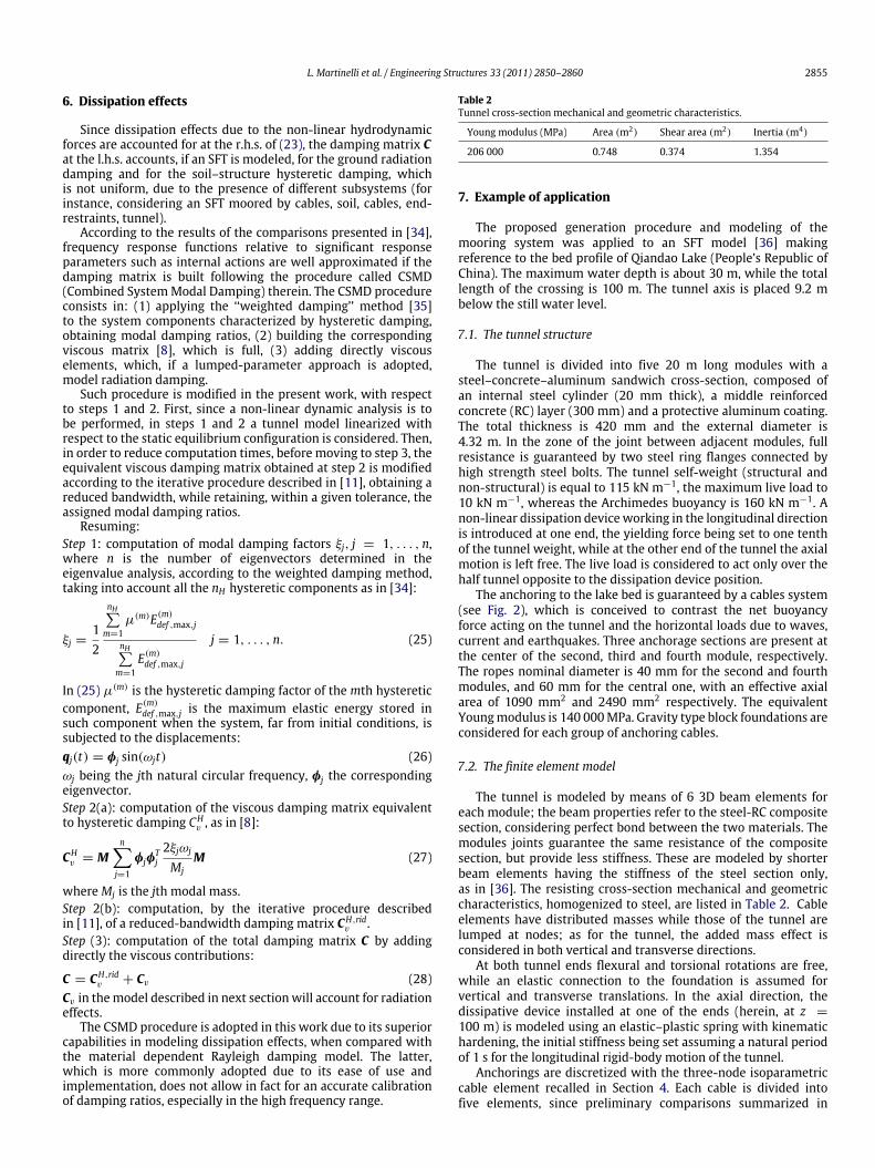
The anchoring to the lake bed is guaranteed by a cables system(see Fig. 2), which is conceived to contrast the net buoyancyforce acting on the tunnel and the horizontal loads due to waves,current and earthquakes. Three anchorage sections are present atthe center of the second, third and fourth module, respectively.The ropes nominal diameter is 40 mm for the second and fourthmodules, and 60 mm for the central one, with an effective axialarea of 1090 mm2 and 2490 mm2 respectively. The equivalentYoungmodulus is 140 000MPa. Gravity type block foundations areconsidered for each group of anchoring cables.

7.2. The finite element model

The tunnel is modeled by means of 6 3D beam elements foreach module; the beam properties refer to the steel-RC compositesection, considering perfect bond between the two materials. Themodules joints guarantee the same resistance of the compositesection, but provide less stiffness. These are modeled by shorterbeam elements having the stiffness of the steel section only,as in [36]. The resisting cross-section mechanical and geometriccharacteristics, homogenized to steel, are listed in Table 2. Cableelements have distributed masses while those of the tunnel arelumped at nodes; as for the tunnel, the added mass effect isconsidered in both vertical and transverse directions.

At both tunnel ends flexural and torsional rotations are free,while an elastic connection to the foundation is assumed forvertical and transverse translations. In the axial direction, thedissipative device installed at one of the ends (herein, at z =

100 m) is modeled using an elastic–plastic spring with kinematichardening, the initial stiffness being set assuming a natural periodof 1 s for the longitudinal rigid-body motion of the tunnel.

Anchorings are discretized with the three-node isoparametriccable element recalled in Section 4. Each cable is divided intofive elements, since preliminary comparisons summarized in

2856 L. Martinelli et al. / Engineering Structures 33 (2011) 2850–2860

Fig. 2. Scheme of the tunnel model.

Section 4.3 showed that such discretization is generally adequatein avoiding fictitious compressions. The connection betweenthe beams modeling the tunnel and the cables end nodes isimposed with rigid link elements, so that torsional effects areconsidered. Soil–structure interaction is taken into account byassuming a lumped-parameter approach. Thus six springs, placedat the centroid of the foundation–ground interface, model the soiltranslational and rotational stiffness, while six linear dashpots,acting in parallel to the springs, account for elastic wave radiation.The springs and dashpots approximate the impedance of ahomogeneous half-space [37], having a shear modulus equal to100 000 kPa, a Poisson coefficient of 0.33 and a mass density equalto 2000 kgm−3. It is assumed that the abutments have dimensionssimilar to those of the foundation blocks.

The damping matrix equivalent to the hysteretic effects ofelastic elements is assembled according to the procedure outlinedin Section 6. Different hysteretic damping ratios have beenconsidered for the tunnel, the end-restraints, the cables and theground (0.05, 0.05, 0.03, 0.03 respectively). From the tunnelmodel,linearized with respect to the static equilibrium configuration,200 vibration modes have been extracted in order to apply steps1 and 2 of the procedure. The first natural frequencies togetherwith a synthetic description of the associated mode shapes, asdetected by visual inspection [2], are listed in Table 3. Then, beforeapplying step 3, that is before adding viscous damping, modelingthe radiation effect, the dampingmatrix half-bandwidth is reducedfrom 469 to 386 degrees of freedom, while the stiffness half-bandwidth is instead equal to 81.

7.3. Seismic loading

A set of acceleration time histories, on average compatible withthe EN 1998 horizontal and vertical response spectra for a soil typeC , were generated with the procedure described in Section 3 andthe parameters listed in Table 1.With reference to Eq. (4), the shearwaves velocity is set equal to vs = 2500 m s−1 and two valuesof the incoherence factor, taken as α = 0.20 and α = 0.65, areconsidered; the former value leads to a rather high correlation.With reference to Eq. (1), t0 was chosen as 12.5% of the generatedlength of the signal (20 s), tn as t0 + tmax, where tmax = 10 s. Thetime step is equal to 0.01 s.

Table 3Linearized tunnel model: natural frequencies and synthetic description of theassociated mode shape (T transverse, V vertical, L longitudinal, C cables, Ffoundations).

Mode number 1 2 3 4 5Mode shape TF VTF L VF FCNatural frequency [Hz] 0.677 0.928 1.097 1.111 1.454Mode number 6 7 8 9 10

Mode shape FC TC VC C C

Natural frequency [Hz] 1.554 1.879 2.013 2.102 2.103Mode number 11 12 13 14 15Mode shape C C CF C CNatural frequency [Hz] 2.107 2.108 2.348 2.430 2.431Mode number 16 17 18 19 20

Mode shape C C C C C

Natural frequency [Hz] 2.449 2.449 3.497 3.497 3.515

The acceleration time historieswere generated along the tunnelat the positions of the anchorage points (0, 30, 50, 70, 100 m).The seismic motion propagates along the longitudinal direction ofthe tunnel, while its variability in the direction transverse to thetunnel is neglected, due to the small distance between the cableanchorages.

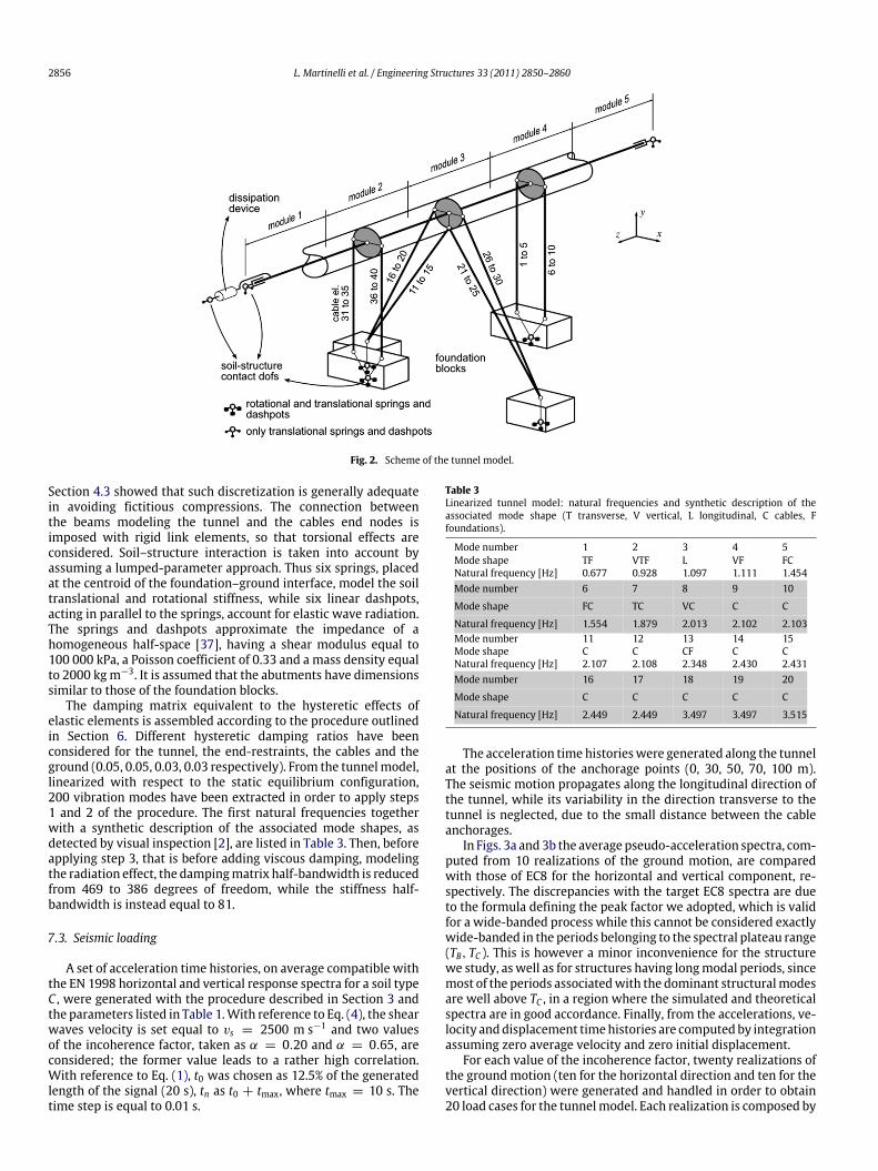
In Figs. 3a and3b the average pseudo-acceleration spectra, com-puted from 10 realizations of the ground motion, are comparedwith those of EC8 for the horizontal and vertical component, re-spectively. The discrepancies with the target EC8 spectra are dueto the formula defining the peak factor we adopted, which is validfor a wide-banded process while this cannot be considered exactlywide-banded in the periods belonging to the spectral plateau range(TB, TC ). This is however a minor inconvenience for the structurewe study, aswell as for structures having longmodal periods, sincemost of the periods associatedwith the dominant structuralmodesare well above TC , in a region where the simulated and theoreticalspectra are in good accordance. Finally, from the accelerations, ve-locity anddisplacement timehistories are computedby integrationassuming zero average velocity and zero initial displacement.

For each value of the incoherence factor, twenty realizations ofthe groundmotion (ten for the horizontal direction and ten for thevertical direction) were generated and handled in order to obtain20 load cases for the tunnelmodel. Each realization is composed by

L. Martinelli et al. / Engineering Structures 33 (2011) 2850–2860 2857

Fig. 3a. Comparison of the average spectrum from 10 generated groundmotions with that of EC8 (left) for the horizontal component, and (right) for the vertical componentα = 0.625.

Fig. 3b. Comparison of the average spectrum from 10 generated groundmotions with that of EC8 (left) for the horizontal component, and (right) for the vertical componentα = 0.2.

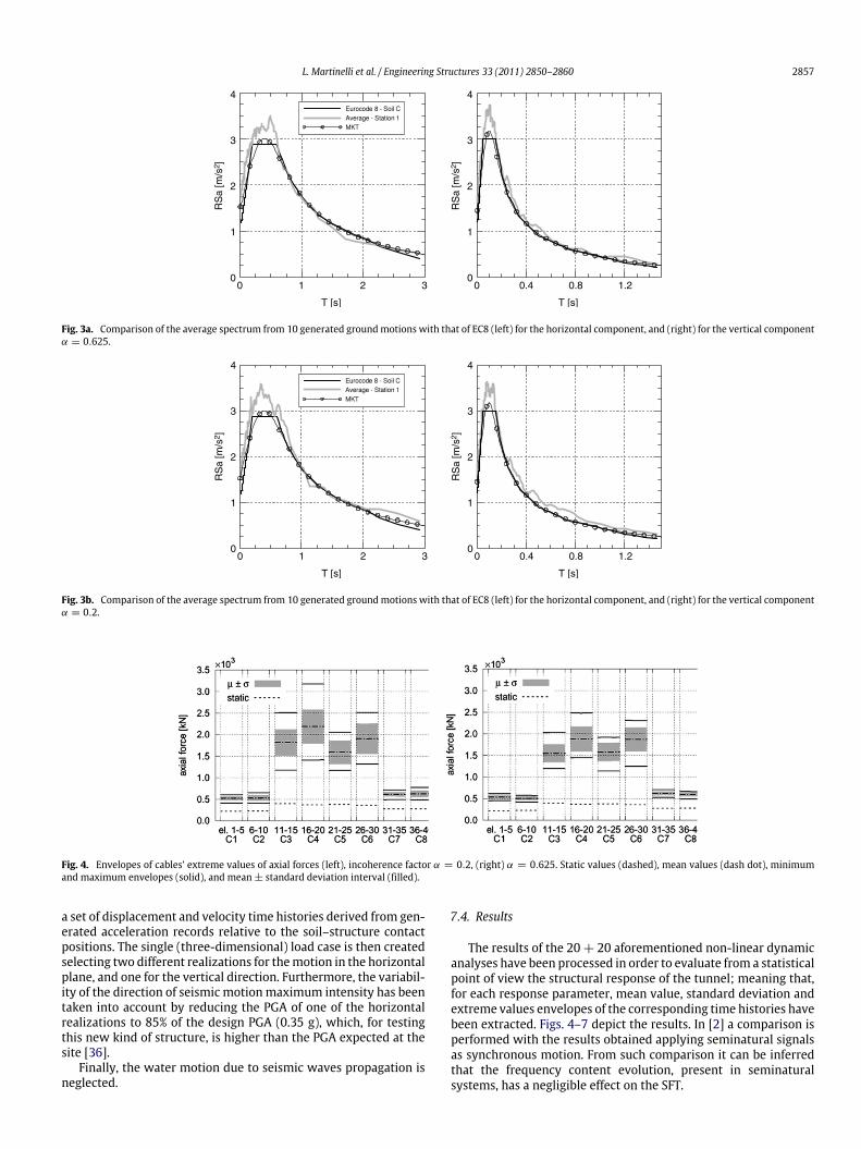
Fig. 4. Envelopes of cables’ extreme values of axial forces (left), incoherence factor α = 0.2, (right) α = 0.625. Static values (dashed), mean values (dash dot), minimumand maximum envelopes (solid), and mean ± standard deviation interval (filled).

a set of displacement and velocity time histories derived from gen-erated acceleration records relative to the soil–structure contactpositions. The single (three-dimensional) load case is then createdselecting two different realizations for themotion in the horizontalplane, and one for the vertical direction. Furthermore, the variabil-ity of the direction of seismic motionmaximum intensity has beentaken into account by reducing the PGA of one of the horizontalrealizations to 85% of the design PGA (0.35 g), which, for testingthis new kind of structure, is higher than the PGA expected at thesite [36].

Finally, the water motion due to seismic waves propagation isneglected.

7.4. Results

The results of the 20 + 20 aforementioned non-linear dynamicanalyses have been processed in order to evaluate from a statisticalpoint of view the structural response of the tunnel; meaning that,for each response parameter, mean value, standard deviation andextreme values envelopes of the corresponding time histories havebeen extracted. Figs. 4–7 depict the results. In [2] a comparison isperformed with the results obtained applying seminatural signalsas synchronous motion. From such comparison it can be inferredthat the frequency content evolution, present in seminaturalsystems, has a negligible effect on the SFT.

2858 L. Martinelli et al. / Engineering Structures 33 (2011) 2850–2860

Fig. 5. Envelopes of extreme values of positive and negative tunnel bending moments about the horizontal axis x, (left) incoherence factor α = 0.2, (right) α = 0.625.Static values (dashed), mean values (dash dot), minimum and maximum envelopes (solid), and mean ± standard deviation interval (filled).

Fig. 6. Envelopes of extreme values of positive and negative tunnel bending moments about the vertical axis y, (left) incoherence factor α = 0.2, (right) α = 0.625. Meanvalues (dash dot), minimum and maximum envelopes (solid), and mean ± standard deviation interval (filled).

Fig. 7. Envelopes of extreme values of positive and negative tunnel axial forces, (left) incoherence factor α = 0.2, (right) α = 0.625. Mean values (dash dot), minimum andmaximum envelopes (solid), and mean ± standard deviation interval (filled).

Fig. 4 depicts the envelopes of the axial forces of the cables; werecall here that elements 1 to 5 belong to cable 1, elements 6 to 10to cable 2, and so on. Cable 1 and 2 restrain sections S1, cables 3,4, 5 and 6 the central section S2 while cables 7 and 8 Section S3.Section S1 is closer to the free end while section S3 to the end withthe dissipative device.

For all the sections S1, S2 and S3, in these analysis the effect of alarger value of α is generally to diminish the scatter of the results.Median values remain about the same or decrease in some cables.

Fig. 5 depicts the envelopes of the extremevalues of the bendingmoment in the tunnel about the horizontal axis x.

Here, in static conditions, a negative (hogging) moment occursalong the tunnel. The shape of the bending moment distributionreflects the peculiarity of the adopted cable configuration. Infact, the non-linear behavior of the cables restraining section S2provides a flexible elastic bilateral/almost unilateral restraint forthe horizontal/vertical motion respectively. When tensioned orloosened, the cables couple the horizontal and vertical motion of

the tunnel at this section. As also confirmed by 3D animations ofthe SFT motion, under an horizontal motion the central sectionis also subject to a downward vertical displacement, since thetensioned cables are inclined and their non-linear behavior is takeninto account. The vertical cables restraining sections S1 and S3do not provide a similar downward displacement. This down-pullingmechanism and the buoyancy of the tunnel are responsiblefor the high negative (hogging) values of bending moments andfor the reduction of the maximum positive (sagging) bendingmoment at section S2 (Fig. 5). Moreover, the envelope of positivebending moment is distributed more evenly, since the tunnel ismore effectively restrained in the upward direction and behaves,under the inertia and buoyancy forces, like a four spans beam onelastic supports. The effect of a larger value of α is to increasethe asymmetry of the results. Median values slightly decrease inmodulus.

Fig. 6 shows the distribution of the bending moment aboutthe vertical axis y. This is similar to that associated to a uniformbeam vibrating according to the first mode shape, and is due to the

L. Martinelli et al. / Engineering Structures 33 (2011) 2850–2860 2859

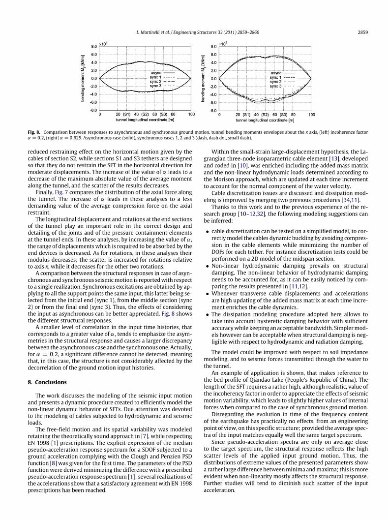
Fig. 8. Comparison between responses to asynchronous and synchronous ground motion, tunnel bending moments envelopes about the x axis, (left) incoherence factorα = 0.2, (right) α = 0.625. Asynchronous case (solid), synchronous cases 1, 2 and 3 (dash, dash dot, small dash).

reduced restraining effect on the horizontal motion given by thecables of section S2, while sections S1 and S3 tethers are designedso that they do not restrain the SFT in the horizontal direction formoderate displacements. The increase of the value of α leads to adecrease of the maximum absolute value of the average momentalong the tunnel, and the scatter of the results decreases.

Finally, Fig. 7 compares the distribution of the axial force alongthe tunnel. The increase of α leads in these analyses to a lessdemanding value of the average compression force on the axialrestraint.

The longitudinal displacement and rotations at the end sectionsof the tunnel play an important role in the correct design anddetailing of the joints and of the pressure containment elementsat the tunnel ends. In these analyses, by increasing the value of α,the range of displacementswhich is required to be absorbed by theend devices is decreased. As for rotations, in these analyses theirmodulus decreases; the scatter is increased for rotations relativeto axis x, while it decreases for the other two rotations.

A comparison between the structural responses in case of asyn-chronous and synchronous seismicmotion is reportedwith respectto a single realization. Synchronous excitations are obtained by ap-plying to all the support points the same input, this latter being se-lected from the initial end (sync 1), from the middle section (sync2) or from the final end (sync 3). Thus, the effects of consideringthe input as asynchronous can be better appreciated. Fig. 8 showsthe different structural responses.

A smaller level of correlation in the input time histories, thatcorresponds to a greater value of α, tends to emphasize the asym-metries in the structural response and causes a larger discrepancybetween the asynchronous case and the synchronous one. Actually,for α = 0.2, a significant difference cannot be detected, meaningthat, in this case, the structure is not considerably affected by thedecorrelation of the ground motion input histories.

8. Conclusions

The work discusses the modeling of the seismic input motionand presents a dynamic procedure created to efficiently model thenon-linear dynamic behavior of SFTs. Due attention was devotedto the modeling of cables subjected to hydrodynamic and seismicloads.

The free-field motion and its spatial variability was modeledretaining the theoretically sound approach in [7], while respectingEN 1998 [1] prescriptions. The explicit expression of the medianpseudo-acceleration response spectrum for a SDOF subjected to aground acceleration complying with the Clough and Penzien PSDfunction [8] was given for the first time. The parameters of the PSDfunctionwere derivedminimizing the differencewith a prescribedpseudo-acceleration response spectrum [1]; several realizations ofthe accelerations show that a satisfactory agreement with EN 1998prescriptions has been reached.

Within the small-strain large-displacement hypothesis, the La-grangian three-node isoparametric cable element [13], developedand coded in [10], was enriched including the added mass matrixand the non-linear hydrodynamic loads determined according tothe Morison approach, which are updated at each time incrementto account for the normal component of the water velocity.

Cable discretization issues are discussed and dissipation mod-eling is improved by merging two previous procedures [34,11].

Thanks to this work and to the previous experience of the re-search group [10–12,32], the following modeling suggestions canbe inferred:

• cable discretization can be tested on a simplified model, to cor-rectlymodel the cables dynamic buckling by avoiding compres-sion in the cable elements while minimizing the number ofDOFs for each tether. For instance discretization tests could beperformed on a 2D model of the midspan section.

• Non-linear hydrodynamic damping prevails on structuraldamping. The non-linear behavior of hydrodynamic dampingneeds to be accounted for, as it can be easily noticed by com-paring the results presented in [11,12].

• Whenever transverse cable displacements and accelerationsare high updating of the added mass matrix at each time incre-ment enriches the cable dynamics.

• The dissipation modeling procedure adopted here allows totake into account hysteretic damping behavior with sufficientaccuracywhile keeping an acceptable bandwidth. Simplermod-els however can be acceptable when structural damping is neg-ligible with respect to hydrodynamic and radiation damping.

The model could be improved with respect to soil impedancemodeling, and to seismic forces transmitted through the water tothe tunnel.

An example of application is shown, that makes reference tothe bed profile of Qiandao Lake (People’s Republic of China). Thelength of the SFT requires a rather high, although realistic, value ofthe incoherency factor in order to appreciate the effects of seismicmotion variability, which leads to slightly higher values of internalforces when compared to the case of synchronous ground motion.

Disregarding the evolution in time of the frequency contentof the earthquake has practically no effects, from an engineeringpoint of view, on this specific structure; provided the average spec-tra of the input matches equally well the same target spectrum.

Since pseudo-acceleration spectra are only on average closeto the target spectrum, the structural response reflects the highscatter levels of the applied input ground motion. Thus, thedistributions of extreme values of the presented parameters showa rather large difference betweenminima andmaxima; this ismoreevident when non-linearity mostly affects the structural response.Further studies will tend to diminish such scatter of the inputacceleration.

2860 L. Martinelli et al. / Engineering Structures 33 (2011) 2850–2860

Acknowledgments

The authors wish to thank Prof. F. Perotti of the Department ofStructural Engineering, Politecnico di Milano, for the discussionson the relevant topics of this researchwork. Financial support fromMIUR (under PRIN 2005), from the ‘‘Ponte di Archimede’’ company,and from the University of Brescia is gratefully acknowledged.

Appendix

Variables quoted in formulas (13) and (14)

A = ζsω31ω2

ζ1ω

31 + 4ζ 2

1 ζ2ω21ω2 + 4ζ1

ζ 21 + ζ 2

2

ω1ω

22

+1 + 4ζ 2

1

ζ2ω

32

+ ω2

1

ζ1ζ2ω

41

+ 4ζ 21

ζ 22 + ζ 2

s

ω3

1ω2 + 2ζ1ζ2−1 + 2ζ 2

2

+ 4ζ 2s + ζ 2

1

2 + 8ζ 2

s

ω2

1ω22 + 4

ζ 21 ζ 2

2

+4ζ 4

1 +1 + 4ζ 2

1

ζ 22

ζ 2s

ω1ω

32

+ ζ1ζ21 + 16ζ 2

1 ζ 2s

ω4

2

ωs

+ 2ζsω1ζ1ω

21 +

1 + 4ζ 2

1

ζ2ω1ω2 + 4ζ 3

1 ω22

×2ζ 2

1 ω1ω2 +−1 + 2ζ 2

2 + 2ζ 2s

ω1ω2 + 2ζ1ζ2

×ω2

1 + ω22

ω2

s + 4ζ1ζ2

ζ 21 + ζ 2

s

ω4

1

+4ζ 4

1 ζ 22 +

ζ 22 + ζ 2

1

1 + 4ζ 2

2

ζ 2s

ω3

1ω2

+ ζ1ζ24ζ 4

1 + ζ 2s + ζ 2

1

−2 + 4ζ 2

2 + 8ζ 2s

ω2

1ω22

+4ζ 41

ζ 22 + ζ 2

s

ω1ω

32 + ζ 3

1 ζ2ω42

ω3

s

+ ζs1 + 4ζ 2

1

ζ2ω

31 + ζ1

×1 + 16ζ 2

1 ζ 22

ω2

1ω2 + 16ζ 41 ζ2ω1ω

22 + 4ζ 3

1 ω32

ω4

s (A.1)

B = 2ζ1ζ2ζs×ω4

1 + 4ζ1ζ2ω31ω2 + 2

−1 + 2ζ 2

1 + 2ζ 22

ω2

1ω22

+ 4ζ1ζ2ω1ω32 + ω4

2

ω4

1 + 4ζ1ζsω31ωs

+ 2−1 + 2ζ 2

1 + 2ζ 2s

ω2

1ω2s + 4ζ1ζsω1ω

3s + ω4

s

×ω4

2 + 4ζ2ζsω32ωs + 2

−1 + 2ζ 2

2 + 2ζ 2s

ω2

2ω2s

+ 4ζ2ζsω2ω3s + ω4

s

(A.2)

C = ζsω41ω

32

ζ1ω

21 +

1 + 4ζ 2

1

ζ2ω1ω2 + 4ζ 3

1 ω22

+ 4ζ 2

s ω31ω

22 (ζ2ω1 + ζ1ω2)

ζ1ω

21 +

1 + 4ζ 2

1

× ζ2ω1ω2 + 4ζ 3

1 ω22

ωs

+ 2ζsω21ω2

2ζ1ζ 2

2 ω41 + ζ2

−1 +

2 + 8ζ 2

1

ζ 22 + ζ 2

s

× ω3

1ω2

+ ζ1−1 + 4ζ 2

2 + 2ζ 2s + ζ 2

1

2 + 8ζ 2

2

1 + 4ζ 2

s

ω2

1ω22

+ 2ζ 21 ζ2

1 + 4ζ 2

1

1 + 4ζ 2

s

ω1ω

32 + 4ζ 3

1

×−1 + 2ζ 2

1 + 2ζ 2s

ω4

2

ω2

s

+ ω1ζ1ζ2ω

51 + 4ζ 2

2

ζ 2s + ζ 2

1

1 + 4ζ 2

s

ω4

1ω2

+ 2ζ1ζ2−1 + 2ζ 2

2 + 4ζ 2s + ζ 2

1

2 + 8ζ 2

s

1 + 4ζ 2

2

× ω3

1ω22 + 4ζ 2

1

ζ 2s + ζ 2

2

1 + 32ζ 2

1 ζ 2s

ω2

1ω32

+ ζ1ζ21 + 16ζ 2

1

1 + 4ζ 2

1

ζ 2s

ω1ω

42 + 16ζ 4

1 ζ 2s ω5

2

× ω3

s + ζs

1 + 4ζ 21

ζ2ω

51 + 4ζ1

1 + 8ζ 2

1

ζ 22 ω4

1ω2

+ 4ζ 21 ζ2

1 + 4ζ 2

1

1 + 4ζ 2

2

ω3

1ω22 + ζ1

×1 + 16ζ 2

1

1 + 4ζ 2

1

ζ 22

ω2

1ω32

+ 32ζ 41 ζ2ω1ω

42 + 4ζ 3

1 ω52

ω4

s

+ 4ζ 31 ζ2

ω4

1 + 4ζ1ζ2ω31ω2 + 2

−1 + 2ζ 2

1 + 2ζ 22

× ω2

1ω22 + 4ζ1ζ2ω1ω

32 + ω4

2

ω5

s . (A.3)

References

[1] Eurocode 8. Design of structures for earthquake resistance. Part 1: Generalrules, seismic actions and rules for buildings. EN 1998–1, 2005.

[2] Martinelli L, Barbella G, Feriani A. Multi-support seismic input and responseof submerged floating tunnels anchored by cables. Technical Report N.6/2010,DICATA, Università degli Studi di Brescia, 2010.

[3] Zerva A, Zervas V. Spatial variation of seismic ground motions: an overview.Appl Mech Rev 2002;55(1):271–96.

[4] Der Kiureghian A, Neuenhofer A. Response spectrum method for multi-support seismic excitations. Earthq Eng Struct Dyn 1992;21:713–40.

[5] Kaul MK. Stochastic characterization of earthquakes through their responsespectrum. Earthq Eng Struct Dyn 1978;6:497–509.

[6] Christian JT. Generating seismic design power spectral density functions.Earthq Spectra 1989;5:351–68.

[7] Monti G, Nuti C, Pinto PE. Nonlinear response of bridges under multisupportexcitation. J Struct Eng 1996;1147–59.

[8] Clough RW, Penzien J. Dynamics of structures. New York, NY: McGraw-Hill;1975.

[9] Martinelli L,MulasMG, Perotti F. The seismic response of concentrically bracedmoment-resisting frames. Earthq Eng Struct Dyn 1996;25:1275–99.

[10] Martinelli L, Perotti F. Numerical analysis of the non-linear dynamic behaviourof suspended cables under turbulentwind excitation. Internat J Struct StabilityDynam 2001;1:207–33.

[11] Fogazzi P, Perotti F. The dynamic response of seabed anchored floating tunnelsunder seismic excitation. Earthq Eng Struct Dyn 2000;29:273–95.

[12] Di Pilato M, Perotti F, Fogazzi P. 3D dynamic response of submerged floatingtunnels under seismic and hydrodynamic excitation. Eng Struct 2008;30:268–81.

[13] Desai YM, Popplewell N, Shah A, Buragohain DN. Geometric nonlinear analysisof cable supported structures. Computer & Structures 1988;29(6):1001–9.

[14] Priestley MB. Power spectral analysis of non-stationary random processed.J Sound Vib 1967;6(1):68–97.

[15] Wang J, Fan L, Qian S, Zhou J. Simulations of non-stationary frequency contentand its importance to seismic assessment of structures. Earthq Eng Struct Dyn2002;31:993–1005.

[16] Gupta ID, Trifunac MD. A note on the nonstationarity of seismic response ofstructures. Eng Struct 2000;23:1567–77.

[17] Gupta ID, Trifunac MD. Defining equivalent stationary PSDF to account fornonstationarity of earthquake ground motion. Soil Dyn Earthq Eng 1998;17:89–99.

[18] Amin M, Ang AH-S. Nonstationary stochastic model of earthquake motions.J Eng Mech Div 1968;94(2):559–83. ASCE.

[19] Abrahamson NA. Generation of spatially incoherent strong motion timehistories. In: Earthquake engineering, tenth world conference. Rotterdam:Balkema; 1992. p. 845–9.

[20] Harichandran RS, Vanmarcke E. Stochastic variation of earthquake groundmotion in space and Time. ASCE J Eng Mech 1986;112:154–74.

[21] Abrahamson NA. Estimation of seismic wave coherency and rupture velocityusing SMART-1 strong motion array recordings. Report no. UCB/EERC-85-02,EERC, Univ. of California at Berkeley, CA, 1985.

[22] Abrahamson NA, Scheider JF, Stepp JC. Empirical spatial coherency functionsfor applications to soil–structure interaction analysis. Earthq Spectra 1991;7:1–28.

[23] Luco JE,Wong HL. Response of a rigid foundation to a spatially random groundmotion. Earthq Eng Struct Dyn 1986;14:891–908.

[24] Loh CH, Yeh YT. Spatial variation and stochastic modelling of seismicdifferential ground movement. Earthq Eng Struct Dyn 1988;15:583–96.

[25] Hao H, Oliveira CS, Penzien J. Multiple-station ground motion processing andsimulation based on SMART-1 array data. Nucl Eng Des 1989;111:293–310.

[26] Shinozuka M. Monte Carlo solution of structural dynamics. Comput Struct1972;2:855–74.

[27] Shinozuka M, C.M. Jan. Digital simulation of random processes and itsapplications. J Sound Vib 1972;25(1):111–28.

[28] Shinozuka M. Stochastic fields and their digital simulation, for publication inlecture notes: stochastic methods in structural mechanics. CISM, Udine, Italy:August 28–30, 1985.

[29] Vanmarcke EH. Structural response to earthquakes. In: Lomnitz C, editor.Seismic risk and engineering decision. New York: McGraw-Hill; 1977.p. 287–337.

[30] Lagarias JC, Reeds JA, Wright MH, Wright PE. Convergence properties of theNelder-Mead simplex method in low dimensions. SIAM J Optim 1998;9(1):112–47.

[31] Chakrabarti SK. Hydrodynamics of offshore structures. computational me-chanics publications. Springer-Verlag; 1987.

[32] Barbella G, Di Pilato M, Feriani A. Effects of the anchoring systems on thedynamic behaviour of the submerged floating structures (SFT). In: AIMETA2007, XVIII Congresso AIMETA di Meccanica Teorica e Applicata, Brescia,11–14 settembre 2007, ed. Starrylink, Brescia, Italy, 2007, CD-ROM, P. 12.

[33] Hilber HM, Hughes TJR, Taylor RL. Improved numerical dissipation for time-integration algorithms in structural dynamics. Earthq Eng Struct Dyn 1977;5:283–93.

[34] Feriani A, Perotti F. The formation of viscous dampingmatrices for the dynamicanalysis of M.D.O.F. systems. Earthq Eng Struct Dyn 1996;25:689–709.

[35] Roesset JM, Whitman RV, Dobry R. Modal analysis for structures withfoundation interaction. ASCE J Struct Div 1973;99:399–415.

[36] Mazzolani FM, Landolfo R, Faggiano B, Esposito M, Perotti F, Barbella G.Structural analyses of the submerged floating tunnel prototype in QiandaoLake (PR of China). Adv Struct Eng 2008;11(4):439–54.

[37] Sieffert JG, Cevaer F. Handbook of impedance functions-surface foundations.Ouest ed. Presses Academiques; 1992.