a numerical study - homepage |...
TRANSCRIPT
Analysis of the Effect of Flow Rate on the DopplerContinuity Equation for Stenotic Orifice Area Calculations
A Numerical Study
Curt G. DeGroff, MD; Robin Shandas, PhD; Lilliam Valdes-Cruz, MD
Background—Flow-rate dependencies of the Doppler continuity equation are addressed in this study.Methods and Results—By use of computational fluid dynamic (CFD) software with turbulence modeling, three-
dimensional axisymmetric models of round stenotic orifices were created. Flow simulations were run for various orificearea sizes (0.785, 1.13, 1.76, and 3.14 cm2) and flow rates (0.37 to 25.0 L/min). Reynolds numbers ranged from 100to 8000. Once adequate convergence was obtained with each simulation, the location of the vena contracta wasdetermined. For each run, maximum and average velocities across the cross section of the vena contracta were tabulatedand vena contracta cross-sectional area (effective orifice area) determined. The difference between the maximumvelocity and the average velocity at the vena contracta was smallest at high-flow states, with more of a difference atlow-flow states. At lower-flow states, the velocity vector profile at the vena contracta was parabolic, whereas athigh-flow states, the profile became more flattened. Also, the effective orifice area (vena contracta cross-sectional area)varied with flow rate. At moderate-flow states, the effective orifice area reached a minimum and expanded at low- andhigh-flow states, remaining relatively constant at high-flow states.
Conclusions—We have shown that significant differences exist between the maximum velocity and the average velocityat the vena contracta at low flow rates. A likely explanation for this is that viscous effects cause lower velocities at theedges of the vena contracta at low flow rates, resulting in a parabolic profile. At higher-flow states, inertial forcesovercome viscous drag, causing a flatter profile. Effective orifice area itself varies with flow rate as well, with thesmallest areas seen at moderate-flow states. These flow-dependent factors lead to flow rate-dependent errors in theDoppler continuity equation. Our results have strong relevance to clinical measurements of stenotic valve areas by useof the Doppler continuity equation under varying cardiac output conditions. (Circulation. 1998;97:1597-1605.)
Key Words: echocardiography • stenosis • blood flow
rphe impetus for assessing valve areas by Doppler tech-J. niques arose from the fact that Doppler-estimated pres-
sure gradients across stenotic valves derived from the sim-plified Bernoulli equation are a flow-dependent index ofstenosis severity.1 Valve area measurement methods usingDoppler techniques were developed as an attempt to providea flow-independent assessment of valve stenosis. Originally,a modified form of the Gorlin and Gorlin equation2 was usedin the Doppler quantification of valve areas.3 Later, thecontinuity equation was introduced4 as an alternative Dopplermethod to estimate valve areas, and it has since become themost commonly used technique.5"14
Nonetheless, the assumption that the Doppler continuityequation is flow independent has not been proved and may beerroneous. Although some investigators have observed amarked flow dependence of valve areas computed from theDoppler continuity equation in the clinical setting,6-7 others
have reported no dependence,8'12 and still others have seenresults varying according to whether low or high flow ratesare used in in vitro flow models.5 Clinical studies examiningthe effect of increasing flow volume through exercise ordobutamine infusion on Doppler-calculated valve areas havealso been performed.7'9'12 Many of these investigators havefound variations in Doppler-calculated valve area as a resultof changing flow conditions and conclude that there may bea flow dependence inherent in this method.
The purpose of this investigation was to use numericalmodeling experimentation to (1) determine whether the venacontracta cross-sectional area, called the "effective" orificearea, changes with flow rate; (2) determine whether orificeareas derived from the Doppler continuity equation accu-rately measure effective orifice areas; and (3) determinewhether the results of the Doppler continuity equation areflow dependent and if so provide explanations for such
Received June 24, 1997; revision received November 10, 1997; accepted December 1, 1997.From the University of Colorado Health Sciences Center, The Children's Hospital, Denver, Colo.Presented in part at the 69th Annual Scientific Sessions of the American Heart Association, New Orleans, La, November 11-14, 1996, and published
in abstract form (Circulation. 1997;96(suppl I):I-471).Correspondence to Curt G. DeGroff, MD, Cardiovascular Flow Dynamics Laboratory, University of Colorado Health Science Center, The Children's
Hospital, 1056 E 19th Ave, B-100, Denver, CO 80218.E-mail [email protected]© 1998 American Heart Association, Inc.
by guest on June 4, 2018http://circ.ahajournals.org/
Dow
nloaded from

1598 Flow Rate and Doppler Continuity Equation
Figure 1. Streamlines through an orifice. Streamlines are linesdrawn in a flow field such that they are always tangent (parallel)to direction of flow. Vena contracta represents a contraction inedges of flow streamlines as they move through an orifice.
dependencies by study of the basic fluid dynamics around astenotic orifice.
In this study, we use numerical experimentation to studythe fluid dynamics around stenotic orifices. Numerical meth-ods allow for a measurement window of the flow dynamicsaround such orifices, which is more precise than otherexperimental techniques, such as in vitro models.
Theoretical Considerations
Vena ContractaFig 1 shows schematically the flow dynamics around astenotic orifice. Streamlines are lines drawn within a flowfield that are always parallel to the direction of flow. Thevena contracta represents a contraction in the edges of theflow streamlines as they move through an orifice.15 Fororifices without a smoothly tapering proximal geometry,inertia prevents proximal streamlines entering from the sidefrom changing direction instantly; in this region, thesestreamlines are directed almost perpendicular to the generalflow direction. As the flow passes through the orifice, thestreamlines change direction to run parallel to the main flowdirection but not before "squeezing" the main flow andcausing a constriction in the cross-sectional area of flowimmediately distal to the orifice. The mechanism that causesthis reduction in distal flow area has been called the venacontracta effect.15 The resulting constricted area (cross-sec-tional area of the vena contracta) is the effective orifice areareflecting the actual area available for flow, which is usuallysmaller than the true orifice area.916 Flow separation justdistal to the orifice causes a recirculation zone to form.Through the middle of the recirculation zone, the mainstream"fresh" flow continues to accelerate from the orifice to itshighest velocity, presumably where the cross-sectional areaof the mainstream flow is narrowest (ie, at the vena con-tracta). Past the vena contracta, blood decelerates again to fillthe vessel. Velocity and pressure vary inversely along thecenterline of blood flow through the orifice. Proximal to theorifice, pressures are high and velocities are low. Approach-ing the vena contracta, pressures drop and velocities increase.Past the vena contracta, in what is called the pressurerecovery zone, pressures rise toward their original magnitudeand velocities decrease.6'17'18
O ADCE ~ Qreference' » Doppler •
Doppler Continuity EquationThe Doppler continuity equation is derived from the conceptsof conservation of mass (continuity equation)15 and thecontrol volume theory,15 whereby flow rate through a refer-ence point (Qreference) and through an orifice along a flowstream must be equal.1 We assume there is a means toaccurately measure flow rate through a reference location.The Doppler continuity equation method assumes a uniformvelocity profile along the cross section of the orifice (VDoppier).The Doppler continuity equation orifice area (OADCE) is givenas
(1)
Typically in clinical practice, when there is pulsatile flow, thevelocity (VDoppler) used in the Doppler continuity equation isthe peak continuous-wave (CW) spectral Doppler velocityused in conjunction with a reference peak flow rate (Qreference)-Because CW Doppler records all velocities along its samplebeam, and the highest velocities along a properly alignedsample beam through a stenotic orifice are thought to be at thevena contracta, the Doppler continuity equation is measuringthe cross-sectional area of the vena contracta, called theeffective orifice area (at peak flow), and not the true orificearea.6
Often in clinical practice, the velocity (VDoppler) used in theDoppler continuity equation is the temporal mean of thehighest recorded CW velocities through a pulsatile cycle (inconjunction with a reference mean flow rate, Qreference)- Thesetemporal means are generally obtained by measuring veloc-ity-time integrals.1 In this case, the Doppler continuity equa-tion is measuring a mean vena contracta cross-sectional areaand not the true orifice area, because (1) the highest velocitiesalong a properly aligned sample beam through a stenoticorifice are thought to be at the vena contracta and (2) themean CW velocity is a temporal mean of the highestvelocities recorded along that sample beam.
Because of the constriction of flow at the vena contracta,this effective orifice area is generally smaller than the trueorifice area (as in Fig 1) and reflects the actual area availablefor flow through the orifice.9'18
The assumption of a uniform velocity through the crosssection of the vena contracta (where the maximum velocityobtained by CW Doppler is assumed to be representative ofthe velocities over the entire cross section of the venacontracta) may not hold at certain flow states. If this assump-tion of a flat velocity profile is erroneous, inaccuracies will beintroduced into the Doppler continuity equation.
Methods
Numerical ModelingNumerical modeling flow experimentation consists of several stages:(1) grid generation, (2) specification of fluid properties and boundaryconditions, (3) acquisition of flow solution, and (4) analysis offlow-data results. A software package from CFD Research was usedin the numerical modeling experimentation. This software packagewas chosen because of superior qualities offered in (1) grid construc-tion, (2) range of CFD solution schemes, (3) range of turbulencemodel selections, (4) visualization and analysis tools, and (5)technical support offered through CFD Research.
by guest on June 4, 2018http://circ.ahajournals.org/
Dow
nloaded from
DeGroff et al April 28, 1998 1599
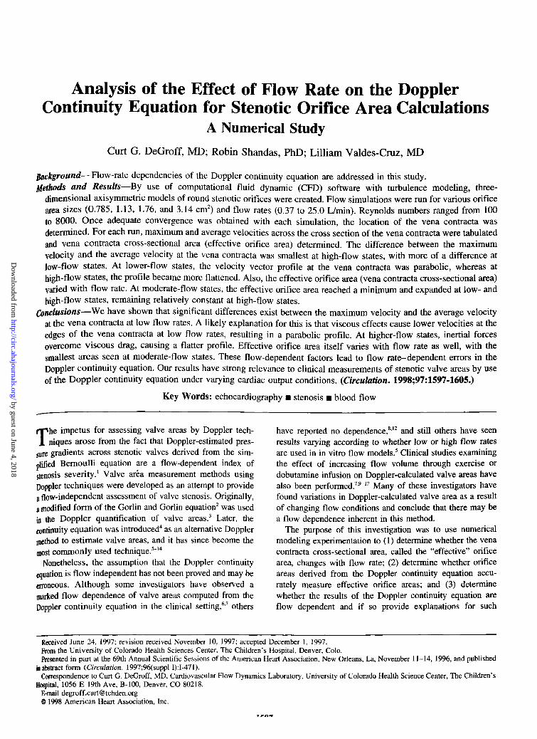
Figure 2. Grid of numerical model used in flow experiments.Inlet chamber is 5 cm long and 27.5 cm in diameter. Outletchamber is 11.25 cm long and 27.5 cm in diameter. Round ste-notic orifices with diameters ranging between 1.0 and 2.5 cmwere placed between inlet and outlet chambers. Width of orificewas 0.1 cm.
Grid GenerationGrid generation is the division of a flow domain (eg, a stenotic valveand the surrounding vessel structure) into a number of smallnonoverlapping subdomains called finite control volumes. CFD-GEOM grid generation software was used to create all of ourthree-dimensional axisymmetric grids.
Fig 2 shows the grid used in our steady-flow experiments. Theinlet chamber was 5 cm in length and 27.5 cm in diameter. The outletchamber was 11.25 cm in length and 27.5 cm in diameter. The widthof the orifice was 0.1 cm. These dimensions were chosen so thatresults could be directly compared with results obtained from our invitro model with these dimensions. Round stenotic orifices withdiameters of 1.0, 1.2, 1.5, and 2.0 cm (giving orifice areas of 0.785,1.13,1-76, and 3.14 cm2, respectively) were placed between the inletand outlet chambers.
Fluid Properties and Boundary ConditionsAll models had fixed boundaries (ie, noncompliant vessel walls).Blood was assumed to be a viscous, incompressible Newtonian fluidof density p=1060 kg/m3 and kinematic viscosity i^=4xlO~6 m2/s.Flow rates (6 to 400 mL/s, or 0.37 to 25 L/min) were prescribed bysetting uniform flow velocities at the inlet boundary. Because ofcomputing hardware constraints (ie, size of grids required), not allflow rates were run through all orifices. Reynolds numbers rangedfrom 100 to 8000.
Flow SolutionGrids were fed into a finite-volume computational fluid dynamics(CFD) analysis package (CFD-ACE) by use of laminar and turbu-lence modeling. The finite-volume numerical algorithm consists ofthree steps19'21: integration of the governing equations of fluid flow(Appendix) over all the control volumes in the flow domain,conversion of these integral equations into a system of algebraicequations (called discretization), and solution of the algebraic equa-tions by an iterative method called SIMPLEC.22"24 We used asecond-order-accurate central differencing discretization scheme19'21
available in CFD-ACE. The performance of CFD-ACE in cardio-vascular applications has previously been well documented.25"29
A solution was considered proper once adequate convergence wasobtained. At each iteration, CFD-ACE calculates a "residual" foreach variable (variables defined in the governing equations of fluidflow, see Appendix) for all control volumes. A residual is thedifference in value of a variable in a control volume from one
Blood Plow
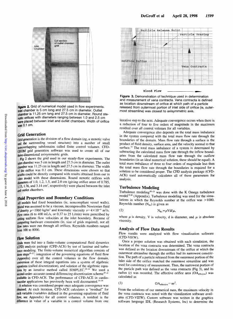
Figure 3. Demonstration of technique used in determinationand measurement of vena contracta. Vena contracta is definedas location downstream of orifice at which path of a particlereleased from outermost portion of inlet side of orifice (ie, outer-most streamline) was closest to axisymmetric axis.
iterative step to the next. Adequate convergence occurs when there isa reduction of four to five orders of magnitude in the maximumresidual over all control volumes for all variables.
Adequate convergence also depends on the total mass imbalancein the system compared with the total mass flow rate through theboundaries of the domain. Mass flow rate through a surface is theproduct of fluid density, surface area, and the velocity normal to thatsurface.15 The total mass imbalance of a system is determined bysubtracting the calculated mass flow rate through the inflow bound-aries from the calculated mass flow rate through the outflowboundaries (in an ideal numerical solution, these should be equal). Atotal mass imbalance of three to four orders of magnitude less thanthe total mass flow rate through the boundaries is required for asolution to be considered proper. The CFD analysis package (CFD-ACE) used automatically calculates all of these parameters foranalysis.
Turbulence ModelingTurbulence modeling19-21 was done with the K Omega turbulencemodel19'20 (Appendix). Turbulence modeling was used for the simu-lations in which the Reynolds number at the orifice was >1000.Reynolds number (NRe) is given as
(2) NRe=pVd/|Lt,
where p is density, V is velocity, d is diameter, andviscosity.
is absolute
Analysis of Flow Data ResultsFlow results were analyzed with flow visualization software(CFD-VIEW).
Once a proper solution was obtained with each simulation, thelocation of the vena contracta was determined. The vena contractawas defined as the location downstream of the orifice at which theoutermost streamline through the orifice had its narrowest constric-tion. The path of a particle released from the outermost portion of theinlet side of the orifice matched the outermost streamline and wasused for consistency of measurement. Thus, the narrowest portion ofthe particle path was defined as the vena contracta (Fig 3), and itsradius (r) was recorded. The effective orifice area (OAeffective) wascalculated as
(3) OAeffective— TTT .
From the solutions of our numerical runs, the maximum velocity inthe vena contracta was noted with the visualization software avail-able (CFD-VIEW). Custom software was written in the graphicssoftware language IDL (Research Systems, Inc) to determine the
by guest on June 4, 2018http://circ.ahajournals.org/
Dow
nloaded from
1600 Flow Rate and Doppler Continuity Equation
Vena Contracta Velocity Profile
(a)
O . 3 7 L/min
34% Differencebetween Maximum and Mean Velocity
6% Differencebetween Maximum and Mean velocity
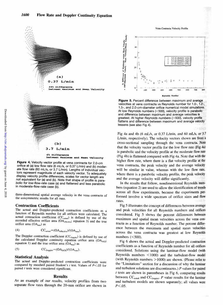
Figure 4. Velocity vector profile at vena contracta for 2.0-cmorifice at (a) low flow rate (6 ml_/s, or 0.37 L/min) and (b) moder-ate flow rate (60 mL/s, or 3.7 L/min). Lengths of individual vec-tors represent magnitude of each velocity vector. To adequatelydisplay velocity profile differences, scales for vector length arenot equivalent for (a) and (b). Note that shape of profile is para-bolic for low-flow-rate case (a) and flattened and less parabolicin moderate-flow-rate case (b).
three-dimensional spatial average velocity in the vena contracta ofthe axisymmetric results for all runs.
Contraction CoefficientsThe actual and Doppler-predicted contraction coefficients as afunction of Reynolds number for all orifices were calculated. Theactual contraction coefficient (CCactual) is defined by use of therecorded effective orifice area (OAeffective; equation 3) and the trueorifice area (OA^) as
(4) CCactual=(OAeffective)/(OAtrue).
The Doppler contraction coefficient (€0^^) is defined by use ofthe calculated Doppler continuity equation orifice areaequation 1) and the true orifice area (OA^) as
(5) CCDoppte=(OADCE)/(OAlrae).
Statistical AnalysisThe actual and Doppler-predicted contraction coefficients werecompared by standard paired Student's t test. Values of /><.05 forpaired t tests were considered significant.
ResultsAs an example of our results, velocity profiles from twoseparate flow rates through the 20-mm orifice are shown in
s*5I
.
onA
V
1.0 c1 ? r1 S r2.0 c
m diameterm diameterm diameterm diameter
orificeorificeorificeorifice
Reynolds Number
Figure 5. Percent difference between maximum and averagevelocities at vena contracta vs Reynolds number for 1.0-, 1.2-,1.5-, and 2.0-cm-diameter orifice numerical model simulations.At low Reynolds numbers (<500), velocity profile is parabolicand difference between maximum and average velocities isgreatest. At higher Reynolds numbers (>500), velocity profileflattens and difference between maximum and average velocitylessens (see also Fig 4).
Fig 4a and 4b (6 mL/s, or 0.37 L/min, and 60 mL/s, or 3.7L/min, respectively). The velocity vectors shown are from across-sectional sampling through the vena contracta. Notethat the velocity vector profile for the low flow rate (Fig 4a)is parabolic and the velocity profile at the moderate flow rate(Fig 4b) is flattened compared with Fig 4a. Note that with thehigher flow rate, where there is a flat velocity profile at thevena contracta, the peak velocity and the average velocitywill be similar in value, whereas with the low flow rate,where there is a parabolic velocity profile, the peak velocityand the average velocity will differ significantly.
In the results that follow, nondimensional Reynolds num-bers (equation 2) are used to allow the identification of trendsacross all flow experiments, because the experiments per-formed involve a wide spectrum of orifice sizes and flowrates.
Fig 5 illustrates the concept of differences between averageand peak velocities for all Reynolds numbers and orificesconsidered. Fig 5 shows the percent differences betweenmaximum and spatial mean velocities across the vena con-tracta as a function of Reynolds number. The percent differ-ence between the maximum and spatial mean velocitiesacross the vena contracta was greatest at low Reynoldsnumbers (<500).
Fig 6 shows the actual and Doppler-predicted contractioncoefficients as a function of Reynolds number for all orificesconsidered. Solutions using the laminar-flow model (withReynolds numbers <1000) and the turbulent-flow model(with Reynolds numbers >1000) are shown. (Please refer tothe "Limitations" section for a discussion of why the laminarand turbulent solutions are discontinuous.) P values for pairedt tests are shown in parentheses in Fig 6, comparing resultsbetween CCactual and CCr^e,. P value results for the laminarand turbulent models are shown separately; all values wereP<.05.
by guest on June 4, 2018http://circ.ahajournals.org/
Dow
nloaded from
DeGroff et al April 28, 1998 1601
1.0 cm Diameter Orifice
(Anatomic Orifice Area = 0.785 cm2)B
(p = 0.048)
Reynolds Number
1.5 cm Diameter Orifice
(Anatomic Orifice Area = 1.766 cm2)
(p = 0.019)
1.2 cm Diameter Orifice
(Anatomic Orifice Area =1.13 cm2)
(p = 0.041)
2000 3000 5000 6000
Reynolds Number
2.0 cm Diameter Orifice
(Anatomic Orifice Area = 3.14 cm2)
Reynolds Number Reynolds Number
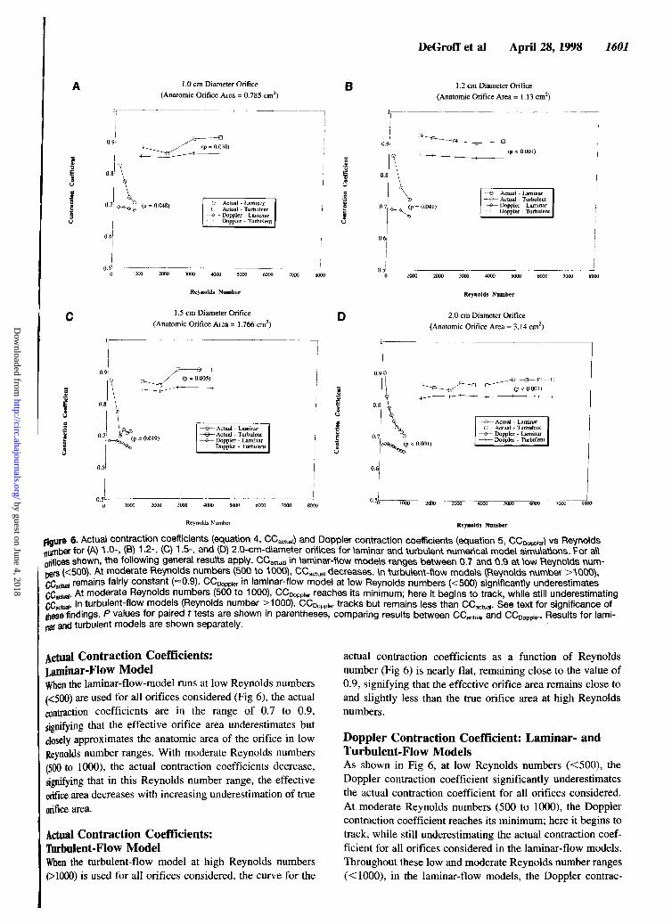
figure 6. Actual contraction coefficients (equation 4, CCactuai) and Doppler contraction coefficients (equation 5, CCDopptev) vs Reynoldpumber for (A) 1 .0-, (B) 1 .2-, (C) 1 .5-, and (D) 2.0-cm-diameter orifices for laminar and turbulent numerical model simulations. For all
spu . , . , . , . . a l lorifices shown, the following general results apply. CCactuai in laminar-flow models ranges between 0.7 and 0.9 at low Reynolds num-bers (<500). At moderate Reynolds numbers (500 to 1000), CCactual decreases. In turbulent-flow models (Reynolds number >AOOO),
i remains fairly constant (~0.9). CCD0ppier in laminar-flow model at low Reynolds numbers (<500) significantly underestimatesi- At moderate Reynolds numbers (500 to 1000), CCDoppier reaches its minimum; here it begins to track, while still underestimatingi- In turbulent-flow models (Reynolds number >1000), CCDoppler tracks but remains less than CCactua,. See text for significance of
these findings. P values for paired t tests are shown in parentheses, comparing results between CCactual and CCDoppier. Results for lami-nar and turbulent models are shown separately.
Actual Contraction Coefficients:Laminar-Flow ModelWhen the laminar-flow-model runs at low Reynolds numbers(<500) are used for all orifices considered (Fig 6), the actualcontraction coefficients are in the range of 0.7 to 0.9,signifying that the effective orifice area underestimates butclosely approximates the anatomic area of the orifice in lowReynolds number ranges. With moderate Reynolds numbers(500 to 1000), the actual contraction coefficients decrease,signifying that in this Reynolds number range, the effectiveorifice area decreases with increasing underestimation of trueorifice area.
Actual Contraction Coefficients:Turbulent-Flow ModelWhen the turbulent-flow model at high Reynolds numbers(>1000) is used for all orifices considered, the curve for the
actual contraction coefficients as a function of Reynoldsnumber (Fig 6) is nearly flat, remaining close to the value of0.9, signifying that the effective orifice area remains close toand slightly less than the true orifice area at high Reynoldsnumbers.
Doppler Contraction Coefficient: Laminar- andTurbulent-Flow ModelsAs shown in Fig 6, at low Reynolds numbers (<500), theDoppler contraction coefficient significantly underestimatesthe actual contraction coefficient for all orifices considered.At moderate Reynolds numbers (500 to 1000), the Dopplercontraction coefficient reaches its minimum; here it begins totrack, while still underestimating the actual contraction coef-ficient for all orifices considered in the laminar-flow models.Throughout these low and moderate Reynolds number ranges(<1000), in the laminar-flow models, the Doppler contrac-
by guest on June 4, 2018http://circ.ahajournals.org/
Dow
nloaded from
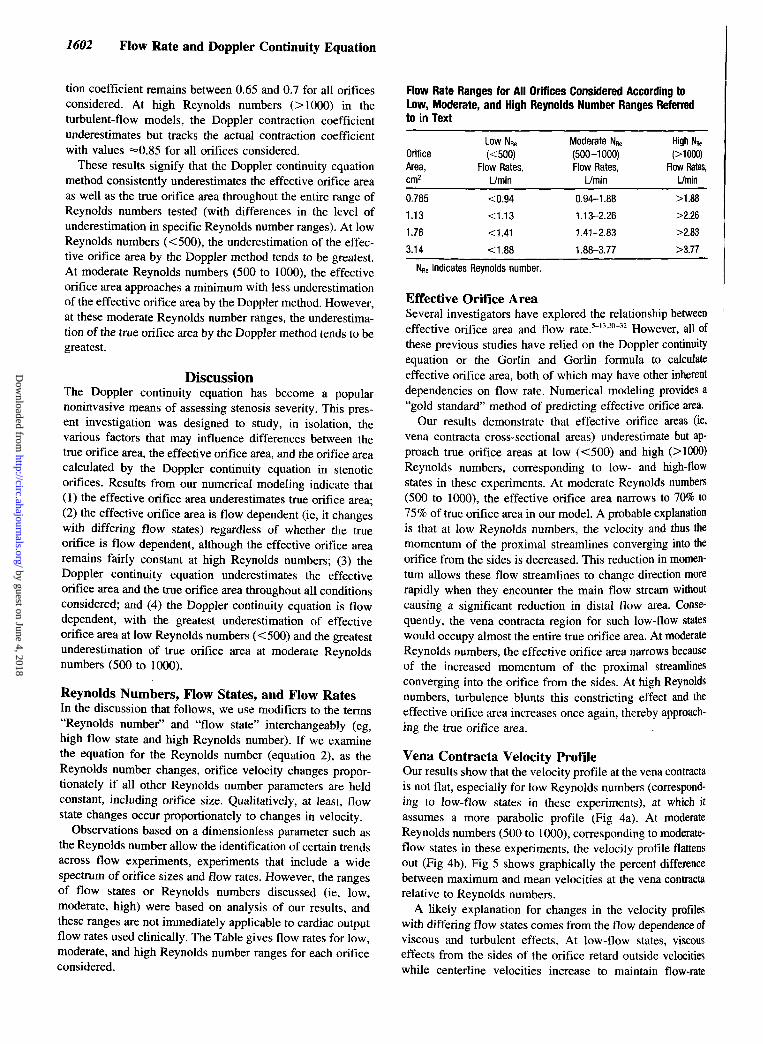
1602 Flow Rate and Doppler Continuity Equation
tion coefficient remains between 0.65 and 0.7 for all orificesconsidered. At high Reynolds numbers (>1000) in theturbulent-flow models, the Doppler contraction coefficientunderestimates but tracks the actual contraction coefficientwith values =«0.85 for all orifices considered.
These results signify that the Doppler continuity equationmethod consistently underestimates the effective orifice areaas well as the true orifice area throughout the entire range ofReynolds numbers tested (with differences in the level ofunderestimation in specific Reynolds number ranges). At lowReynolds numbers (<500), the underestimation of the effec-tive orifice area by the Doppler method tends to be greatest.At moderate Reynolds numbers (500 to 1000), the effectiveorifice area approaches a minimum with less underestimationof the effective orifice area by the Doppler method. However,at these moderate Reynolds number ranges, the underestima-tion of the true orifice area by the Doppler method tends to begreatest.
DiscussionThe Doppler continuity equation has become a popularnoninvasive means of assessing stenosis severity. This pres-ent investigation was designed to study, in isolation, thevarious factors that may influence differences between thetrue orifice area, the effective orifice area, and the orifice areacalculated by the Doppler continuity equation in stenoticorifices. Results from our numerical modeling indicate that(1) the effective orifice area underestimates true orifice area;(2) the effective orifice area is flow dependent (ie, it changeswith differing flow states) regardless of whether the trueorifice is flow dependent, although the effective orifice arearemains fairly constant at high Reynolds numbers; (3) theDoppler continuity equation underestimates the effectiveorifice area and the true orifice area throughout all conditionsconsidered; and (4) the Doppler continuity equation is flowdependent, with the greatest underestimation of effectiveorifice area at low Reynolds numbers (<500) and the greatestunderestimation of true orifice area at moderate Reynoldsnumbers (500 to 1000).
Reynolds Numbers, Flow States, and Flow RatesIn the discussion that follows, we use modifiers to the terms"Reynolds number" and "flow state" interchangeably (eg,high flow state and high Reynolds number). If we examinethe equation for the Reynolds number (equation 2), as theReynolds number changes, orifice velocity changes propor-tionately if all other Reynolds number parameters are heldconstant, including orifice size. Qualitatively, at least, flowstate changes occur proportionately to changes in velocity.
Observations based on a dimensionless parameter such asthe Reynolds number allow the identification of certain trendsacross flow experiments, experiments that include a widespectrum of orifice sizes and flow rates. However, the rangesof flow states or Reynolds numbers discussed (ie, low,moderate, high) were based on analysis of our results, andthese ranges are not immediately applicable to cardiac outputflow rates used clinically. The Table gives flow rates for low,moderate, and high Reynolds number ranges for each orificeconsidered.
Flow Rate Ranges for All Orifices Considered According toLow, Moderate, and High Reynolds Number Ranges Referredto in Text
OrificeArea,cm2
0.785
1.13
1.76
3.14
Low NRe
(<500)Flow Rates,
L/min
<0.94
<1.13
<1.41
<1.88
Moderate NRe
(500-1000)Flow Rates,
L/min
0.94-1 .88
1.13-2.26
1.41-2.83
1.88-3.77
High NRe(>1000)
Flow Rates,L/min
>1.88
>2.26
>2.83
>3.77
NRe indicates Reynolds number.
Effective Orifice AreaSeveral investigators have explored the relationship betweeneffective orifice area and flow rate.5'13'30'32 However, all ofthese previous studies have relied on the Doppler continuityequation or the Gorlin and Gorlin formula to calculateeffective orifice area, both of which may have other inherentdependencies on flow rate. Numerical modeling provides a"gold standard" method of predicting effective orifice area.
Our results demonstrate that effective orifice areas (ie,vena contracta cross-sectional areas) underestimate but ap-proach true orifice areas at low (<500) and high (>1000)Reynolds numbers, corresponding to low- and high-flowstates in these experiments. At moderate Reynolds numbers(500 to 1000), the effective orifice area narrows to 70% to75% of true orifice area in our model. A probable explanationis that at low Reynolds numbers, the velocity and thus themomentum of the proximal streamlines converging into theorifice from the sides is decreased. This reduction in momen-tum allows these flow streamlines to change direction morerapidly when they encounter the main flow stream withoutcausing a significant reduction in distal flow area. Conse-quently, the vena contracta region for such low-flow stateswould occupy almost the entire true orifice area. At moderateReynolds numbers, the effective orifice area narrows becauseof the increased momentum of the proximal streamlinesconverging into the orifice from the sides. At high Reynoldsnumbers, turbulence blunts this constricting effect and theeffective orifice area increases once again, thereby approach-ing the true orifice area.
Vena Contracta Velocity ProfileOur results show that the velocity profile at the vena contractais not flat, especially for low Reynolds numbers (correspond-ing to low-flow states in these experiments), at which itassumes a more parabolic profile (Fig 4a). At moderateReynolds numbers (500 to 1000), corresponding to moderate-flow states in these experiments, the velocity profile flattensout (Fig 4b). Fig 5 shows graphically the percent differencebetween maximum and mean velocities at the vena contractarelative to Reynolds numbers.
A likely explanation for changes in the velocity profileswith differing flow states comes from the flow dependence ofviscous and turbulent effects. At low-flow states, viscouseffects from the sides of the orifice retard outside velocitieswhile centerline velocities increase to maintain flow-rate
by guest on June 4, 2018http://circ.ahajournals.org/
Dow
nloaded from

DeGroff et al April 28, 1998 1603
equity, resulting in a velocity profile that diverges from flat atthe vena contracta. At moderate- and high-flow states, vis-cous effects diminish, allowing turbulence effects to play amore important role. Velocity profiles in turbulent flow areknown to be inherently blunt and flat,33 and our resultsconfirm this. To the best of our knowledge, no previousinvestigations have studied the actual velocity profiles acrossthe vena contracta in stenotic lesions.
Doppler Continuity EquationOur results elucidate two fundamental reasons why thepoppler continuity equation underestimates true orifice areaand is flow dependent. First, because of the vena contractaeffect, the Doppler continuity equation theoretically measuresthe effective orifice area (see "Theoretical Considerations").As we have demonstrated, the effective orifice area itselfunderestimates true orifice area and is flow dependent.Second, the Doppler continuity equation does not accuratelytrack the effective orifice area. The inaccuracies in trackingthe effective orifice area can be explained by the fact that themaximum velocity obtained clinically with CW Doppler andused in the Doppler continuity equation is thought to berepresentative of the spatial average of velocities over theentire cross section of the vena contracta. This holds true onlyin the presence of a flat velocity profile throughout the venacontracta. Any variation from a flat velocity profile will leadto overestimation of the spatial average of velocities andconsequently to an underestimation of orifice area in thepoppler continuity equation, because velocity is in thedenominator (see equation 1).
At low Reynolds numbers (<500), corresponding to low-flow states in these experiments, the effective orifice areaunderestimates the true orifice area and the vena contractavelocity shows a parabolic nonflat profile. Both of theseeffects (especially the parabolic velocity profile) cause thePoppler continuity equation to underestimate the true orificearea.
At moderate Reynolds numbers (500 to 1000), correspond-ing to moderate-flow states in these experiments, the effectiveorifice area begins to succumb to constriction effects, andthere is increasing underestimation of true orifice area. Thevena contracta velocity profile is flatter. Thus, errors fromvelocity profile effects become minimal and changes in theeffective orifice area dominate, causing the Doppler continu-ity equation to continue to underestimate the true orifice area.
At high Reynolds numbers (>1000), corresponding tohigh-flow states in these experiments, the effective orificearea increases because of turbulence effects, and the venacontracta velocity profile continues to be flat. Thus, errorsfrom both of these effects are minimized, and there is lessunderestimation of true orifice area by the Doppler continuityequation.
Clinical ImplicationsThe flow rate dependence of the Doppler continuity equationhas been explored by investigators in the clinical setting byexercise or dobutamine stress echocardiography in aorticstenosis.7'9'12 Most of these studies demonstrate changingDoppler valve areas with varying cardiac outputs. Investiga-
tors who have shown an increase in Doppler valve areas withincreasing flow theorize that the valve leaflets open fartherwhen exposed to the greater pressure gradient.7'9'11 Althoughthis may undoubtedly be part of the explanation, our studieson rigid orifices offer an additional reason for the Dopplerunderestimation of effective orifice area at low cardiacoutputs, which is inherent in the assumptions of the equationitself. These assumptions must be kept in mind when weapply Doppler methods in clinical practice. If treatmentdecisions are to be based on the measurements derived fromthe Doppler continuity equation, understanding these flow-rate dependencies becomes quite important.
LimitationsWith our numerical experimentation tools, we performeddetailed investigations of the flow dynamics through stenoticorifices, which provided a unique means of assessing theaccuracy of the Doppler continuity method. Although thefixed rigid orifices in our model are admittedly a simplifica-tion of a complex three-dimensional structure of a stenoticvalve, they allow isolation of the effects of flow on venacontracta or effective orifice area without the added complex-ity of possible anatomic expansion of a physiological orificeas flow rate increases.7"9'11
Numerical modeling was used because it provides a uniquemedium for detailed examination of the fluid dynamicsaround the vena contracta region. The limitations of allnumerical models include the fact that a selected number ofnumerical solutions should be validated with in vitro models.Preliminary in vitro studies in our laboratory show similarresults for the deviation of the velocity profile away from flatto more parabolic profiles across the vena contracta atlow-flow states as well as changes in effective orifice areafrom low- to moderate-flow states.34 Work is in progresscomparing the velocity vector fields of the numerical and invitro models for further validation of our method.
Numerical modeling over such a wide range of Reynoldsnumbers presents unique problems for any CFD algorithm.Our ranges of Reynolds numbers include modeling laminarflow, transitional flow, and turbulent flow. The decision toturn on turbulence modeling at Reynolds numbers >1000was done with some insight as to when turbulence occurs inthese types of problems.15 However, selecting this turbulencethreshold was still somewhat arbitrary.
A discontinuity between laminar and turbulent modelcontraction coefficients (Fig 6) occurs at this turbulencethreshold. We believe this represents a weakness of the CFDalgorithm we used in predicting results in the transitionalflow range. To the best of our knowledge, this weakness isshared by all CFD algorithms developed to date. A weaknessof a CFD algorithm in predicting results in this transitionalflow range does not negate its results in the laminar andturbulence ranges. Such a sharp discontinuity in the contrac-tion coefficient curves probably does not occur in reality. It ismore likely that there is a much smoother transition from onecurve to the other in the transitional-flow Reynolds numberregion (^lOOO). Overall, however, the finite-volume CFDanalysis package (CFD-ACE) we used provides a robustsolution algorithm, as suggested by the agreement with our in
by guest on June 4, 2018http://circ.ahajournals.org/
Dow
nloaded from
1604 Flow Rate and Doppler Continuity Equation
vitro validation studies to date.34 A complete description ofthe transition from laminar- to turbulent-flow processes isbeyond the scope of this investigation; for further discussion,the reader is referred to Landahl et al.35
Our definition of the vena contracta relies on determiningstreamlines and particle-tracking algorithms. How well thesealgorithms predict the average path of a particle in turbulentflow is a question that we will be addressing in future studies.
Our model considers steady flow. Pulsatile-flow numericalruns were prohibitive in computing-power and time require-ments to obtain solution convergence practically. A relativelydense grid pattern in our model was required for the detailthat was necessary in examining the vena contracta region.Dense grid patterns require relatively small time incrementsin solving for pulsatile flow. Unfortunately, to obtain propernumerical solutions, dense grid patterns and small timeincrements require computational power beyond our presentcapabilities. With this, we elected to run the required densegrid patterns under steady-flow conditions.
We considered flow rates (6 to 400 mL/s, or 0.37 to 25L/min) that allow for comparison to mean and peak flow ratesseen clinically. Strictly speaking, simplifying the analysis ofpulsatile flow by comparing conditions at peak or mean flowstates in a pulsatile system with steady-flow conditions atequivalent flow states is not entirely accurate. Thus, thesesteady-flow experiments do not allow for the direct assess-ment of the ability of the Doppler continuity equation methodto measure the effective orifice area using peak or mean flowrates and velocities under pulsatile conditions. However,these steady-flow experiments have allowed us a uniquewindow into the complexities of the fluid dynamics near astenotic orifice. Further pulsatile-flow studies will be re-quired. In preliminary numerical and in vitro pulsatile-flowexperiments in our laboratory, similar trends in velocityprofiles versus Reynolds number have been noted.
Extending our results to the aortic valve does not accountfor the effects of the aortic walls, which are much closer tothe stenotic orifice than in our model. In addition, we have notexamined errors introduced into the clinically applied Dopp-ler continuity equation as a result of calculations involved inthe determination of the reference flow rate (see equation 1),in which this reference flow rate (Qreference) is typicallydetermined by use of spectral Doppler measurements.
ConclusionsOur results demonstrate the flow dependency of the Dopplercontinuity equation. This flow dependency is due to flow-dependent changes of the effective orifice area (cross-section-al area of the vena contracta) as well as to changes in the venacontracta velocity profile. At low-flow states, the velocityprofile is skewed, causing underestimation of true orificeareas. At moderate-flow states, the velocity profile becomesmore flattened, lessening its effects on orifice area errors;however, the vena contracta (effective orifice area) becomesmore constricted, causing continued underestimation of trueorifice areas. At high-flow states, the velocity profile remainsflattened, and there is less constriction at the vena contracta(ie, greater effective orifice area), causing less underestima-tion of true orifice areas.
The clinical implications of our study are that (1) theunderestimation of true orifice area at low cardiac outputstates by the Doppler continuity equation may lead toerroneous clinical assessments and unnecessary therapeuticinterventions, and (2) results of clinical studies by otherinvestigators that have shown an increase in the Dopplercontinuity equation-calculated valve area with exercise ordobutamine infusion can be explained by fundamentallysound fluid dynamic principles that compound the generallyaccepted explanation of increase in valve leaflet opening.
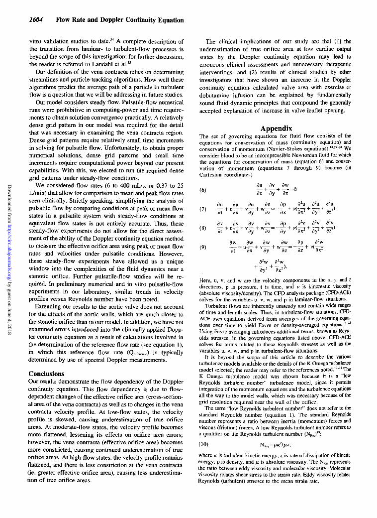
AppendixThe set of governing equations for fluid flow consists of theequations for conservation of mass (continuity equation) andconservation of momentum (Navier-Stokes equations).15'19"21 Weconsider blood to be an incompressible Newtonian fluid for whichthe equations for conservation of mass (equation 6) and conser-vation of momentum (equations 7 through 9) become (inCartesian coordinates)
(6)du dv dw
dx dy dz
du du du du dp d2u d2u
dv dv dv(8) ¥ + Ud7 + Vd7 + W^=~dy-
dv dp d2V d2V d V-j 2
dx dy
(9)dw dw dw dw dp d2W
d2w d2w
Here, u, v, and w are the velocity components in the x, y, and idirections, p is pressure, t is time, and v is kinematic viscosity(absolute viscosity/density). The CFD analysis package (CFD-ACE)solves for the variables u, v, w, and p in laminar-flow situations.
Turbulent flows are inherently unsteady and contain wide rangesof time and length scales. Thus, in turbulent-flow situations, CFD-ACE uses equations derived from averages of the governing equa-tions over time to yield Favre or density-averaged equations.19"21
Using Favre averaging introduces additional terms, known as Reyn-olds stresses, in the governing equations listed above. CFD-ACEsolves for terms related to these Reynolds stresses as well as thevariables u, v, w, and p in turbulent-flow situations.
It is beyond the scope of this article to describe the variousturbulence models available or the details of the K Omega turbulencemodel selected; the reader may refer to the references noted.19"21 TheK Omega turbulence model was chosen because it is a "lowReynolds turbulent number" turbulence model, since it permitsintegration of the momentum equations and the turbulence equationsall the way to the model walls, which was necessary because of thegrid resolution required near the wall of the orifice.
The term "low Reynolds turbulent number" does not refer to thestandard Reynolds number (equation 1). The standard Reynoldsnumber represents a ratio between inertia (momentum) forces andviscous (friction) forces. A low Reynolds turbulent number refers toa qualifier on the Reynolds turbulent number (NRet)
19:
(10) NRet=PK2//*e,
where K is turbulent kinetic energy, e is rate of dissipation of kineticenergy, p is density, and /A is absolute viscosity. The NRe, representsthe ratio between eddy viscosity and molecular viscosity. Molecularviscosity relates shear stress to the strain rate. Eddy viscosity relatesReynolds (turbulent) stresses to the mean strain rate.
by guest on June 4, 2018http://circ.ahajournals.org/
Dow
nloaded from
DeGroff et al April 28, 1998 1605
The K Omega turbulence model requires that the first grid pointfrom a wall must be placed in the laminar sublayer. The laminarsublayer is defined by a location in the grid at which the distancefrom the wall specifies a value of a dimensionless number, y + ,between 0 and 5. y + is a dimensionless number at the walls, defined
(H) y4
where y equals the distance to closest grid point from the wall and UT
is the friction velocity [UT= (rw/p)1/2, where TW is wall shear stress].CFD-ACE automatically calculates y + (equation 11) at the walls.
To ensure that the first grid point from any wall was in the viscoussublayer (for those runs requiring turbulence modeling), the grid waschecked (and modified if necessary) for each run so that the value ofy + at the walls was between 0 and 5.15'19
AcknowledgmentThis study was supported in part by a Pilot Grant from TheChildren's Hospital Research Institute, Denver, Colo.
References1. Snider AR, Serwer GA. Echocardiography in Pediatric Heart Disease.
Baltimore, Md: Mosby Year Book; 1990:108.2. Gorlin R, Gorlin SG. Hydraulic formula for calculation of the area of the
stenotic mitral valve, other cardiac valves, and central circulatory shunts.Am Heart J. 1951;41:l-29.
3. Kosturakis D, Allen HD, Goldberg SJ, Sahn DJ, Valdes-Cruz LM. Non-invasive quantification of stenotic semilunar valve areas by Dopplerechocardiography. / Am Coll Cardiol. 1984;3:1256-1262.
4. Skjaerpe T, Hegrenaes L, Hatle L. Noninvasive estimation of valve areain patients with aortic stenosis by Doppler ultrasound and two dimen-sional echocardiography. Circulation. 1985;72:810-818.
5. Otto CM, Pearlman AS, Gardner CL, Enomoto DM, Togo T, Tsuboi H,Ivey TD. Experimental validation of Doppler echocardiographic mea-surement of volume flow through the stenotic aortic valve. Circulation.1988;78:435-441.
6. Dumensil JG, Yoganathan AP. Theoretical and practical differencesbetween the Gorlin formula and the continuity equation for calculatingaortic and mitral valve areas. Am J Cardiol. 1991;67:1268-1272.
7. Burwash IG, Thomas DD, Sadahiro M, Pearlman AS, Verrier ED, Thom-as R, Kraft CD, Otto CM. Dependence of Gorlin formula and continuityequation valve areas on transvalvular volume flow rate in valvular aorticstenosis. Circulation. 1994;89:827-835.
8. Segal J, Lerner DJ, Miller C, Mitchell RS, Alderman EA, Popp RL. Whenshould Doppler-determined valve area be better than the Gorlin formula? Variation in hydraulic constants in low flow states. J Am Coll Cardiol.1987;9:1294-1305.
9. Pascoe RD, Roger VL, Pellikka PA, Seward JB, Tajik AJ. Use ofdobutamine stress echocardiography in patients with aortic stenosis,reduced left ventricular ejection fraction, and low mean transvalvulargradient: preliminary experience. J Am Soc Echocardiog. 1994;7(3-II):S8. Abstract.
10. Vanoverschelde J-L, D'Hondt A-M, De Kock M. Flow-dependence ofaortic stenosis severity during dobutamine infusion: comparison of theGorlin and continuity equations with measurements of aortic valveresistance. Circulation. 1995;92(suppl I):I-464. Abstract.
11. Otto CM, Pearlman AS, Kraft CD, Miyake-Hull CY, Burwash IG,Gardner CJ. Physiologic changes with maximal exercise in asymptomaticvalvular aortic stenosis assessed by Doppler echocardiography. J Am CollCardiol. 1992;20:1160-1167.
12. Casale PN, Palacios IF, Abrascal VM, Harrel L, Davidoff R, WeymanAE, Fifer MA. Effects of dobutamine on Gorlin and continuity equationvalve areas and valve resistance in valvular aortic stenosis. Am J Cardiol.1992;70:1175-1179.
13. Yoganathan AP, Woo YR, Sung HW, Williams FP, Franch RH, JonesMJ. In-vitro hemodynamic characteristics of tissue bioprostheses in theaortic position. J Thorac Cardiovasc Surg. 1986;92:198-209.
14. Dumensil JG, Honos GN, Lemieux M, Beauchemin J. Validation andapplications of mitral prosthetic valvular areas calculated by Dopplerechocardiography. Am J Cardiol. 1990;65:1443-1448.
15. Fox RW, McDonald AT. Introduction to Fluid Mechanics. 4th ed. NewYork, NY: John Wiley & Sons; 1992:98-354.
16. Shandas R, Kwon J, Kringlen M, Jones M, Valdes-Cruz LM. Hysteresisbehavior of stenotic aortic bioprosthesis as a function of flow rate:in-vitro studies. J Am Coll Cardiol. 1996;27(suppl A):233A. Abstract.
17. Lender MS, Shaffer EM, Valdes-Cruz LM, Wiggins JW, Cape EG.Insights into catheter/Doppler discrepancies: a clinical study of congenitalaortic stenosis. Circulation. 1996;94(suppl I):I-415. Abstract.
18. Cape EG, Jones M, Yamada I, VanAuker MD, Valdes-Cruz LM. Turbu-lent/viscous interactions control Doppler/catheter pressure discrepanciesin aortic stenosis: the role of the Reynolds number. Circulation. 1996;94:2975-2981.
19. CFD Research Theory Manual. Version 1.0. Huntsville, Ala: CFDResearch; 1993:9.12-9.13.
20. Wilcox DC. Turbulence Modeling for CFD. La Canada, Calif: DCWIndustries; 1993.
21. Versteeg HK, Malalasekera W. An Introduction to Computational FluidDynamics: The Finite Volume Method. New York, NY: John Wiley &Sons; 1995.
22. Patankar SV, Spalding DB. A calculation procedure for heat, mass andmomentum transfer in three-dimensional parabolic flows. Int J Heat MassTransfer. 1972;15:1787-1806.
23. Van Doormal JP, Raithby GD. Enhancements of the SIMPLE method forpredicting incompressible fluid flows. Numerical Heat Transfer. 1984;7:147-163.
24. Yang HQ, Habchi SD, Przekwas AJ. A general strong conservationformulation of Navier-Stokes equations in non-orthogonal curvilinearcoordinates. AIAA J. 1994;32:936-941.
25. Makhijani VB, Yang HQ, Singhal AK, Hwang NC. An experimental-numerical analysis of MHV cavitation: effects of leaflet squeezing andrebound. J Heart Valve Dis. 1994;3(suppl l):35-48.
26. Makhijani VB, Siegel JM, Hwang NC. Numerical analysis ofsqueeze-flow in tilting disc mechanical heart valves. J Heart Valve Dis.1996;5:97-103.
27. Makhijani VB, Yang HQ, Dionne PJ, Thubrikar MJ. Three-dimensionalcoupled fluid-structure simulation of pericardial bioprosthetic aortic valvefunction. ASAIO J. 1997;43:M387-M392.
28. Sukumar R, Athavale MM, Makhijani VB, Przekwas AJ. Application ofcomputational fluid dynamics techniques to blood pumps. Artif Organs.1996;20:529-533.
29. Bergman HL, Siegel JM, Oshinski JN, Pettigrew RI, Ku DN. Computa-tional simulation of magnetic resonance angiograms in stenotic vessels:effect of stenosis severity. Adv Bioeng. 1996;33:295-296.
30. Voelker W, Reul H, Nienhaus G, Stelzer T, Schmitz B, Steegers A,Karsch KR. Comparison of valvular resistance, stroke work loss, andGorlin valve area for quantification of aortic stenosis: an in-vitro study ina pulsatile aortic flow model. Circulation. 1995;91:1196-1204.
31. Gorlin R. Calculations of cardiac valve stenosis: restoring an old conceptfor advanced applications. J Am Coll Cardiol. 1987;10:920-922.
32. Cannon SR, Richards KL, Crawford M. Hydraulic estimation of stenoticorifice area: a correction of the Gorlin formula. Circulation. 1985;71:1170-1178.
33. Caro CG, Pedley TJ, Schroter RC, Seed WA. The Mechanics of theCirculation. New York, NY: Oxford University Press; 1978:55-63.
34. Shandas R, Kwon J, Valdes-Cruz LM. In-vitro studies of velocity profileswithin the proximal jet using digital particle image velocimetry: impli-cations for clinical Doppler method. Circulation. 1996;94(suppl I):I-492.Abstract.
35. Landahl MT, Mollo-Christensen E. Turbulence and Random Processes inFluid Mechanics. New York, NY: Cambridge University Press; 1992.
by guest on June 4, 2018http://circ.ahajournals.org/
Dow
nloaded from

Curt G. DeGroff, Robin Shandas and Lilliam Valdes-CruzOrifice Area Calculations: A Numerical Study
Analysis of the Effect of Flow Rate on the Doppler Continuity Equation for Stenotic
Print ISSN: 0009-7322. Online ISSN: 1524-4539 Copyright © 1998 American Heart Association, Inc. All rights reserved.
is published by the American Heart Association, 7272 Greenville Avenue, Dallas, TX 75231Circulation doi: 10.1161/01.CIR.97.16.1597
1998;97:1597-1605Circulation.
http://circ.ahajournals.org/content/97/16/1597the World Wide Web at:
The online version of this article, along with updated information and services, is located on
http://circ.ahajournals.org//subscriptions/
is online at: Circulation Information about subscribing to Subscriptions:
http://www.lww.com/reprints Information about reprints can be found online at: Reprints:
document.
Permissions and Rights Question and Answer Further information about this process is available in therequested is located, click Request Permissions in the middle column of the Web page under Services.the Editorial Office. Once the online version of the published article for which permission is being
can be obtained via RightsLink, a service of the Copyright Clearance Center, notCirculationpublished in Requests for permissions to reproduce figures, tables, or portions of articles originallyPermissions:
by guest on June 4, 2018http://circ.ahajournals.org/
Dow
nloaded from