a numerical study of the effects of wind forcing on the...

Journal of OceanographyVol. 51, pp. 585 to 614. 1995

A Numerical Study of the Effects of Wind Forcingon the Chile Current System

MARY L. BATTEEN, CHIH-PING HU, JEFFREY L. BACON and CRAIG S. NELSON

Department of Oceanography, Naval Postgraduate School, Monterey, CA 93943, U.S.A.

(Received 26 October 1993; in revised form 10 April 1995; accepted 12 April 1995)

A high-resolution, multi-level, primitive equation ocean model is used to examinethe response of the coastal region from 22.5°S to 35°S of the Chile Current Systemto both equatorward and climatological wind forcing. The results from both typesof forcing show that an equatorward surface current, a poleward undercurrent,upwelling, meanders, filaments and eddies develop in response to the predominantequatorward wind forcing. When climatological wind forcing is used, an offshorebranch of the equatorward surface current is also generated. These features areconsistent with available observations of the Chile Current System. The modelresults support the hypothesis that wind forcing is an important mechanism forgenerating currents, eddies and filaments in the Chile eastern boundary currentsystem and in other eastern boundary current regions which have predominantlyequatorward wind forcing.

1. IntroductionThe eastern boundary current (EBC) system off the west coast of Chile is part of the Peru

Humboldt coastal upwelling system, which extends from 5°S to 50°S. This system is influencedpredominantly by equatorward winds throughout the year (Fig. 1). The direction, and to a largedegree the magnitude of the winds, are the result of a semipermanent subtropical high pressuresystem that is similar in nature and behavior to its counterpart in the Northern Hemisphere, theNorth Pacific Subtropical High, as described in Nelson (1977). The South Pacific SubtropicalHigh migrates meridionally with the seasons, reaching its northernmost extent during the australwinter (Figs. 1B and 1C), with its center located roughly at 25°S. As the seasons progress, thehigh pressure system moves southward until its center reaches about 32.5°S during the australsummer (Figs. 1E and 1F).

Because of this migration, maximum values of wind stress (Fig. 1) vary temporally at givenlocations. North of Chile, for example, the maximum wind stress is seen during the austral winter(Figs. 1B and 1C), presumably because the South Pacific Subtropical High reaches its northernmostmigration at that time, and the resulting winds take on more of an alongshore characteristic. Themiddle of the Chilean coastline, in contrast, does not experience maximum wind stress valuesuntil late spring and summer (Figs. 1D and 1E).

The oceanic regime adjacent to the coast of Chile is comprised of several major features (seeFig. 2), including an equatorward surface current called the Chile-Peru Current (CPC) and apoleward undercurrent known as both the Gunther Current and the Peru-Chile Undercurrent(PCU). The climatological CPC is similar to other EBCs in that it is a sluggish (Order (10cm/s)), wide and generally shallow flow moving equatorward along a west coast (Wooster andReid, 1963). Mass transports have been estimated to be ~19 × 106 m3/s (Wooster and Reid, 1963).The primary source of the CPC is, as expected, the West Wind Drift, because the South American

586 M. L. Batteen et al.

continent extends far enough south to intercept at least part of the flow, and divert it towards thenorth. The CPC consists of two equatorward currents (Tchernia, 1980; Gunther, 1936). The outercurrent is usually referred to as the oceanic CPC, which has a maximum depth of ~700 m(Tchernia 1980). The inner surface current is known as the coastal CPC, which extends to ~200m depth (Tchernia, 1980).

Until recently, the PCU had been relatively unexplored. Although Gunther (1936) discussedthe undercurrent that would eventually carry his name, very little additional research wasconducted on the PCU until 1961, when Wooster and Gilmartin (1961) measured it using

Fig. 1. Wind stress fields for the time period A: April–May, B: June–July, C: August–September, D:October–November, E: December–January, and F: February–March. Vectors are scaled in units ofdyne/cm2. Ellipses show areas of large standard errors (after Bakun and Nelson, 1991).

A Numerical Study of the Effects of Wind Forcing on the Chile Current System 587

parachute drogues. Their article sparked a new interest in the region, and soon severalexpeditions set out to study the waters adjacent to the South American coast. Between 1960 and1982 the area was explored by twelve different expeditions (Fonseca, 1989). Results of theexpeditions revealed that the PCU is present all year, has its core at ~150–200 m depth, isprincipally located between the coast and 200 km offshore, has average speeds on the order of10 cm/s, and has a mass transport of ~10 × 106 m3/s (Fonseca, 1989).

Recent observations have shown that, superimposed on the broad, climatological mean flowin this and other EBC regions, such as the California Current System, are highly energetic,mesoscale features such as meanders, eddies and filaments (Mooers and Robinson, 1984). Thesefeatures have been observed during periods of predominantly equatorward winds, which are

Fig. 2. Generalized circulation schematic for the Chile Current System (after Codispoti et al. 1989): Thebroad equatorward Chile-Peru Current (CPC) (solid lines) separates into two branches: the coastalCPC and the oceanic CPC. The coastal CPC overlies the poleward undercurrent, known as the Peru-Chile Undercurrent (PCU) (dashed line). Model Domain: Area of study is a 1152 km (cross-shore) by1280 km (alongshore) box off the coast of Chile.


favorable for upwelling. These observations provide evidence for wind forcing as a possibleimportant mechanism for the formation of currents, meanders, eddies, and filaments in EBCregions.

The Chile Current System offers a unique opportunity to isolate the effects of predominantlyequatorward winds in an EBC system. Since the coastline is relatively straight (see Fig. 2), thereshould be no significant effects of wind forcing with irregular coastline geometry (such as capesand bays). Also, since the topography abruptly drops off the coast to the Peru-Chile Trench, thereshould be no major effects of wind forcing with topography.

In contrast, the other EBC regions that have predominantly equatorward winds, such as thecentral and southern regions of the California Current System, have irregular coastline geometryand topography. Also, in other EBC regions where the coastlines are relatively straight, such asin the northern regions of the California Current System and of the Canary Current System, thewind stress is predominantly equatorward only during the upwelling season, from around Aprilto September. (During the rest of the year, the winds reverse and become predominantlypoleward.) In the EBC region off Western Australia, the winds are predominantly equatorwardand the coastline is relatively straight; however, the thermal forcing is so strong in this region thatthe predominantly observed surface current (the Leeuwin Current) opposes the winds (e.g.,Batteen et al. 1992).

There have been numerous wind forcing models used over the past few decades to modelEBCs, particularly the California Current System. Early work included that of Pedlosky (1974)and Philander and Yoon (1982), who used steady wind stress and transient wind forcing,respectively. Carton (1984) and Carton and Philander (1984) investigated the response ofreduced gravity models to realistic coastal winds. Another series of experiments were done byMcCreary et al. (1987) utilizing a linear model with both transient and steady wind forcing in theCalifornia Current System. In all of these models, relatively weak currents (5–10 cm/s) weregenerated but no eddies or filaments developed.

Batteen et al. (1989) used a primitive equation, multi-level model with biharmonic (ratherthan Laplacian, as used by the previous authors) heat and momentum diffusion which had bothsteady and meridionally varying wind forcing. In both cases, when the baroclinic/barotropicshear between the surface current and undercurrent became strong enough, meanders andfilaments developed. Although this was the first EBC model to simulate meanders and filamentsin the California Current System, no eddies were generated by the end of the 90-day experiments,presumably due to the relatively short simulation time.

The objective of this study is to extend the work of Batteen et al. (1989) by investigating theeffects that both equatorward and climatological wind forcing have on the generation of not onlycurrents, meanders, and filaments, but also eddies, in the Chile Current System. A slightlymodified version of the high-resolution, multi-level, primitive equation model of Batteen et al.(1989) will be used to simulate the effects of wind stress in this region. Longer simulation timesthan 90 days will be used to allow the eddies to be generated and subsequently analyzed.

This paper emphasizes the generation of the currents and eddies due to wind forcing. Themajor structure of the currents is generated early in the experiment; subsequently meanders andeddies develop. The structure of the currents is important prior to the generation of the meandersand eddies, so that is why the eddy energy analysis will be done during the first 180 days of eachexperiment.

The organization of this study is as follows: Section 2 describes the numerical model, theforcing, the specific initial and experimental conditions, and the energy analysis technique. This


technique is used to investigate the dynamical reasons for the generation of eddies in the ChileCurrent System. Section 3 includes an analysis of the results of the modeling experiments, alongwith a comparison of model results with available observations, while Section 4 contains asummary.

2. The Model

2.1 Model description and initial conditionsTo investigate the role of wind forcing on the generation of currents, eddies, and filaments

in the Chile EBC region, the wind stress fields, discussed below, were used to specify the windforcing for a high-resolution, multi-level, primitive equation (PE) model of a baroclinic oceanon a β-plane. The model is based on the hydrostatic, Boussinesq, and rigid lid approximations.The governing equations are defined in Batteen et al. (1989). For the finite differencing, a space-staggered B-scheme (Arakawa and Lamb, 1977) is used in the horizontal. Batteen and Han(1981) have shown that this scheme is appropriate when the grid spacing is approximately on thesame order as, or less than, the Rossby radius of deformation, which meets the criteria of thisstudy. The horizontal grid spacing is 10 km alongshore and 9 km cross-shore, while the internalRossby radius of deformation is ~30 km. In the vertical, the 10 layers are separated by constantz levels at depths of 13, 46, 98, 182, 316, 529, 870, 1416, 2283, and 3656 m. Consistent withHaney (1974), this spacing scheme concentrates more on the upper, dynamically active part ofthe ocean, above the thermocline.

The model domain (Fig. 2) extends off the west coast of Chile, from ~22.5°S to 35°S (1280km alongshore), and from ~72.5°W to 82.5°W (1152 km cross-shore). The eastern boundary ofthe model domain is closed, and has both the tangential and normal components of velocity setto zero. To isolate the role of wind forcing in the generation of eddies, the eastern boundary ismodeled as a straight, vertical wall extending from the surface to 4500 m depth. Theseassumptions are justified since the Chilean coastline is relatively straight and smooth (see Fig.2), the continental shelf is relatively narrow, and the continental slope is steep, dropping fromsea level to over 2000 m depth in a distance of less than 25 km from the coast (Zeigler et al. 1957).The northern, southern and western borders are open boundaries which use a modified versionof the radiation boundary conditions of Camerlengo and O’Brien (1980). Some spatial smoothingis applied in the vicinity of the open boundaries.

The model uses biharmonic lateral heat and momentum diffusion with the same choice ofcoefficients (i.e., 2.0 × 1017 cm4s–1) as in Batteen et al. (1989). Holland (1978) showed that thehighly scale-selective biharmonic diffusion acts predominantly on submesoscales, while Hol-land and Batteen (1986) found that baroclinic mesoscale processes can be damped by Laplacianlateral heat diffusion. As a result, the use of biharmonic lateral diffusion should allow mesoscaleeddy generation via barotropic (horizontal shear) and/or baroclinic (vertical shear) instabilitymechanisms. As in Batteen et al. (1989), weak (0.5 cm2s–1) vertical eddy viscosities and con-ductivities are used. Bottom stress is parameterized by a simplified quadratic drag law (Weatherly,1972), as in Batteen et al. (1989).

The method of solution is straightforward with the rigid lid and flat bottom assumptionsbecause the vertically integrated horizontal velocity is subsequently nondivergent. The verticalmean flow can be described by a stream function which can be predicted from the vorticityequation, while the vertical shear currents can be predicted after the vertical mean flow issubtracted from the original equations. The other variables, i.e., temperature, density, vertical


velocity and pressure, can be explicitly obtained from the thermodynamic energy equation,equation of state, continuity equation, and hydrostatic relation, respectively. Since density isprimarily a function of temperature (e.g., see Wooster and Reid, 1963) and there are no majorsalinity sources or sinks (such as major rivers) in the region being modeled, effects of salinitychanges on density are neglected.

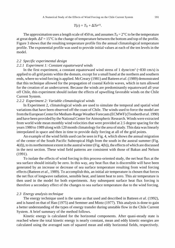
An annual climatological temperature profile (Fig. 3), centered at ~28°S (corresponding tothe middle of the model domain), based on Levitus (1982), was used to represent the initialtemperature conditions for the model domain. An exponential curve was then used to approximatethis. The form of the equation used was:

Fig. 3. Temperature profile (i.e., temperature in degrees Celsius versus depth in meters) used in the model:A smooth exponential curve (solid line) was used to approximate the climatological temperatureprofile (solid line with small circles) computed from Levitus (1982).


T(z) = TB + ∆Tez/h.

The approximation uses a length scale of 450 m, and assumes TB = 2°C to be the temperatureat great depth. ∆T = 15°C is the change of temperature between the bottom and top of the profile.Figure 3 shows that the resulting temperature profile fits the annual climatological temperatureprofile. The exponential profile was used to provide initial values at each of the ten levels in themodel.

2.2 Specific experimental design2.2.1 Experiment 1: Constant equatorward winds

In the first experiment, a constant equatorward wind stress of 1 dyne/cm2 (~830 cm/s) isapplied to all grid points within the domain, except for a small band at the northern and southernends, where no wind forcing is applied. McCreary (1981) and Batteen et al. (1989) demonstratedthat this technique allowed for the propagation of coastal Kelvin waves, which in turn allowedfor the creation of an undercurrent. Because the winds are predominantly equatorward all yearoff Chile, this experiment should isolate the effects of upwelling favorable winds on the ChileCurrent System.2.2.2 Experiment 2: Variable climatological winds

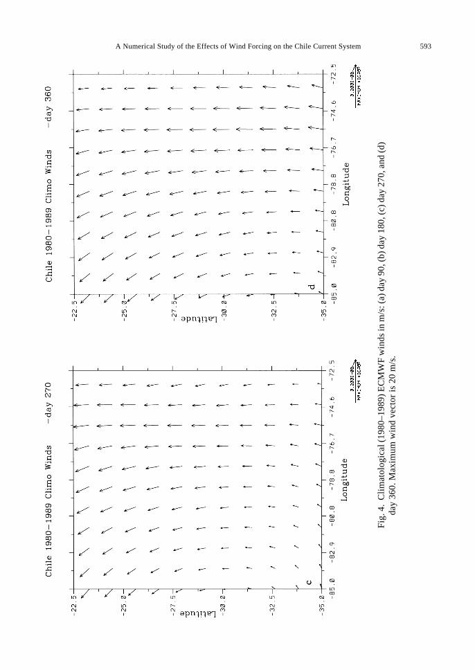
In Experiment 2, climatological winds are used to simulate the temporal and spatial windvariations that have been observed off the coast of Chile. The winds used to force the model arefrom the European Center for Medium-Range Weather Forecasts (ECMWF) (Trenberth et al. 1990)and have been provided by the National Center for Atmospheric Research. Winds were extractedfrom world wide mean monthly wind velocities that were provided at 2.5 degree spacing for theyears 1980 to 1989 along with 120 month climatology for the area of study. This data was linearlyinterpolated in space and then in time to provide daily forcing at all of the grid points.

An example of the wind fields used can be seen in Fig. 4, which shows the annual migrationof the center of the South Pacific Subtropical High from the south in the austral summer (Fig.4(d)), to its northernmost extent in the austral winter (Fig. 4(b)), the effects of which are discussedin the next section. These wind field patterns are consistent with those of Bakun and Nelson(1991).

To isolate the effects of wind forcing in this process-oriented study, the net heat flux at thesea surface should initially be zero. In this way, any heat flux that is discernible will have beengenerated by an increase or decrease of sea surface temperature resulting from wind forcingeffects (Batteen et al., 1989). To accomplish this, an initial air temperature is chosen that forcesthe net flux of longwave radiation, sensible heat, and latent heat to zero. This air temperature isthen used in the model for both experiments. Any subsequent surface heat flux forcing istherefore a secondary effect of the changes to sea surface temperature due to the wind forcing.

2.3 Energy analysis techniqueThe energy technique used is the same as that used and described in Batteen et al. (1992),

and is based on that of Han (1975) and Semtner and Mintz (1977). This analysis is done to gaina better understanding of the types of energy transfer during unstable flow in the Chile CurrentSystem. A brief summary of the method follows.

Kinetic energy is calculated for the horizontal components. After quasi-steady state isreached where the total kinetic energy is nearly constant, mean and eddy kinetic energies arecalculated using the averaged sum of squared mean and eddy horizontal fields, respectively.


Fig

. 4.

Cli

mat

olog

ical

(19

80–1

989)

EC

MW

F w

inds

in m

/s: (

a) d

ay 9

0, (

b) d

ay 1

80, (

c) d

ay 2

70, a

nd (

d)da

y 36

0. M

axim

um w

ind

vect

or is

20

m/s

.


Fig

. 5.

Exp

erim

ent 1

: Sur

face

vel

ocit

y ve

ctor

s in

the

coas

tal r

egio

n at

day

s (a

) 30,

(b) 4

5, (c

) 105

, and

(d)

360.

In

the

velo

city

fie

lds

pres

ente

d (F

igs.

5 a

nd 1

1), t

o av

oid

clut

ter,

vel

ocit

y ve

ctor

s ar

e pl

otte

d at

ever

y th

ird

grid

poi

nt i

n bo

th t

he c

ross

-sho

re a

nd a

long

shor

e di

rect

ions

, an

d ve

loci

ties

les

s th

an 5

cm/s

are

not

plo

tted

. T

he n

umbe

rs a

ssoc

iate

d w

ith

the

high

s in

Fig

s. 6

(c)

and

6(d)

cor

resp

ond

tote

mpe

ratu

re, n

ot v

eloc

ity.

Max

imum

cur

rent

vec

tor

is 8

0 cm

/s.


Next, the available potential energy is calculated and used to determine when a quasi-steady stateis reached and when statistics should be collected. Then, both mean and eddy available potentialenergies are computed. The barotropic and baroclinic energy transfers, defined in Batteen et al.(1992), are used to argue for the type of instability mechanism (e.g., barotropic, baroclinic, ormixed) which leads to the initial eddy generation in each experiment.

3. Results of the ExperimentsExperiments 1 and 2 study the role of wind forcing in the formation of currents and eddies

in the Chile Current System. Experiment 1 uses steady equatorward winds, while Experiment 2uses climatological average (1980–1989) winds.

3.1 Experiment 1: Constant equatorward windsExperiment 1 was forced with a constant equatorward wind stress (1 dyne/cm2), which was

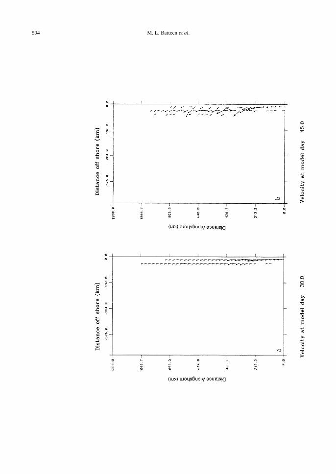
uniform in both the alongshore and cross-shore directions. As expected, the equatorward windforcing resulted in an equatorward surface current along most of the coast (Fig. 5(a)). Thecurrent’s velocities ranged from ~10 to 30 cm/s throughout the duration of the experiment. Thecoastal jet axis was within ~50 km of the coast and extended to ~150 m depth (Fig. 6(a)).

A poleward undercurrent with a core velocity of ~8 cm/s at ~100 to 150 m depth is also seenin Fig. 6(a) below the surface current. The undercurrent extends along the entire coast and isconfined to ~50 km of the coast. Typical velocities for the undercurrent ranged from ~5 to 15cm/s throughout the duration of the experiment.

Along with the equatorward surface current, upwelling also occurred, as seen in Fig. 7(a).Meanders in the equatorward surface current formed by model day 45 and are evident in both thevelocity and temperature plots (Figs. 5(b) and 7(b), respectively). As the meanders intensify, coldupwelling filaments develop along the coast and subsequently extend farther offshore. (Compareday 45 in Fig. 7(b) with day 75 in Fig. 7(c) to see the time evolution.)

More detailed analysis was performed to determine the type of instability mechanism thatcould generate the meander features. Barotropic instability can result from horizontal shear,while baroclinic instability can result from vertical shear in the current. As Fig. 6(a) shows, thereis considerable horizontal and vertical shear between the equatorward surface current and thepoleward undercurrent. As a result, both types of instabilities (mixed), can be present simulta-neously. Energy transfer calculations which consist of barotropic (mean kinetic energy to eddykinetic energy) and baroclinic (mean potential energy to eddy potential energy to eddy kineticenergy) components were performed for the time period (i.e., days 39–60) during which themeanders developed. The results for the instability analyses (Fig. 8) show that both barotropic(Fig. 8(a)) and baroclinic (Fig. 8(b)) instabilities were present in the coastal region of the domain.

By model day 105, the meanders began to form cold core, cyclonic eddies and warm core,anticyclonic eddies, as seen in Figs. 5(c) and 7(d), due to vertical and horizontal shear instabilitiesbetween the equatorward jet and the poleward undercurrent. The eddies initially appeared to beabout 100 km in diameter and extended about 100–200 km off the coast. Subsequently, the eddiespropagated farther offshore with speeds of ~5–10 km/day, consistent with Rossby wavepropagation speeds. The time scales of the eddies are on the order of months.

At the end of the model year, the coastal jet, undercurrent (not shown), meanders and eddies(which have propagated further offshore) are still present (Fig. 5(d)). Upwelling and filamentsare also still discernible (Fig. 7(e)). These features are due to the constant equatorward windforcing, which provides a continual source for the maintenance of the currents and the subsequent


Fig. 6. Experiment 1: Cross-shore section at y ~ 640 km (~29°S) of the meridional component of velocityat day 30 for (a) Experiment 1 and (b) Experiment 2. Solid lines indicate equatorward flow, whiledashed lines indicate poleward flow. The contour interval is 2 cm/s. The maximum equatorwardvelocity is ~20 cm/s at the surface, ~50 km off the coast.


Fig

. 7.

Exp

erim

ent 1

: Sur

face

tem

pera

ture

in th

e co

asta

l reg

ion

at d

ays

(a) 3

0, (b

) 45,

(c) 7

5, (d

) 105

, and

(e) 3

60. T

he c

onto

ur in

terv

al is

0.5

°C. T

he te

mpe

ratu

re d

ecre

ases

tow

ard

the

coas

t. N

ote

the

exis

tenc

eof

upw

elli

ng a

nd m

eand

ers.


Fig

. 8.

E

xper

imen

t 1:

Ene

rgy

tran

sfer

s in

the

coa

stal

reg

ion

of (

a) m

ean

to e

ddy

kine

tic

ener

gy (

i.e.,

baro

trop

ic e

nerg

y tr

ansf

er)

and

(b)

eddy

pot

enti

al t

o ed

dy k

inet

ic e

nerg

y (i

.e.,

the

fina

l st

age

ofba

rocl

inic

ene

rgy

tran

sfer

) fo

r m

odel

day

s 39

to 6

0. T

he c

onto

ur in

terv

al is

10

ergs

cm

–3s–1

.


Fig. 9. Experiment 1: Total (solid line), mean (dashed line), and eddy (dotted line) kinetic energy per unitmass time series for the upper layer over the entire domain for the first 900 days.

Fig. 10. Experiment 1: Time-averaged meridional component of velocity at (a) the surface and (b) ~200m depth. The time averaging is every 3 days from days 33–900. The contour interval is 5 cm/s in (a)and 2.5 cm/s in (b).


Fig

. 11.

Exp

erim

ent 2

: Sur

face

vel

ocit

y ve

ctor

s in

the

coas

tal r

egio

n at

day

s (a

) 30

, (b)

45,

(c)

135

, (d)

180,

(e)

225

, and

(f)

360

. The

num

bers

ass

ocia

ted

wit

h th

e hi

ghs

in F

igs.

10(

d) a

nd 1

0(f)

cor

resp

ond

to te

mpe

ratu

re, n

ot v

eloc

ity.

Max

imum

cur

rent

vec

tor

is 8

0 cm

/s.


development (via barotropic/baroclinic instability mechanisms) of meanders, filaments, andeddies.

Longer experimental runs of three more years show that the system has reached a quasi-steady state (Fig. 9), and that these features, such as the coastal jet (the CPC) and the undercurrent(the PCU), continue to be maintained (Fig. 10). Note that the mean kinetic energy (Fig. 9) remainsfairly constant throughout the experiment. This is expected, since the source for the mean kineticenergy, i.e., the wind forcing, is steady and equatorward. As a result, a quasi-steady equatorwardjet (the CPC) should be present throughout the duration of the experiment. Because of thedominance of eddies in the model domain offshore of the CPC (e.g., see Fig. 5(d)), it is usefulto do time averaging over periods longer than months (the time scale of the eddies) to see thepermanent structure of features in the Chile Current System. To see these structures for the CPCand also the PCU, time averaging every 3 days from days 33–900 of the meridional componentof velocity was taken. The results (Fig. 10) show the presence of a permanent equatorward CPCand poleward PCU, with speeds of ~10–30 cm/s and ~2–10 cm/s, respectively. A comparison ofFigs. 10(a) and 10(b) also shows that there is considerable horizontal and vertical shear in thecurrents.

Since the coastal currents are confined to a narrow region of the model domain (i.e., within90 km of the 1152 km model domain), their contribution to the total kinetic energy shown in Fig.9 is small. The main contribution to the total kinetic energy is the eddy kinetic energy. The growthof eddy kinetic energy seen in Fig. 9 from days 100 to 360 is consistent with the appearance andgrowth of eddies over the same time period (e.g., see Figs. 5(c) and 5(d) for days 105 and 360,respectively). Since the eddies are generated on the offshore side of the coastal currents andsubsequently move slowly westward, they dominate the model domain outside the narrowcoastal current region, resulting in the large contribution to the domain-averaged eddy and totalkinetic energies (Fig. 9).

3.2 Experiment 2: Variable climatological windsExperiment 2 was forced with the climatological average (1980–1989) winds (Fig. 4). An

equatorward surface current was observed all along the coast by model day 30 (Fig. 11(a)) dueto the prevailing equatorward winds. The current’s velocities ranged from ~10 to 30 cm/sthroughout the experiment. The coastal jet axis was within ~50 km of the coast and extended to~250 m depth (Fig. 6(b)). These results are similar to Experiment 1, as expected, since the windsare still predominantly equatorward.

Unlike Experiment 1, an equatorward surface current also develops ~200–300 km offshorebetween days 30 and 45 in the poleward end of the model domain (Fig. 11(b)). The core of thecurrent extends to a depth of ~250 m depth (Fig. 6(b)). From days 90 to 150, it extends along theentire coast (e.g., see Fig. 11(c)). From days 165 to 210, it is strongest in the equatorward endof the domain (e.g., see Fig. 11(d)). It subsequently restrengthens in the poleward end of thedomain by day 225 (Fig. 11(e)). The location of the strongest velocities for this feature appearsto migrate with the center of the South Pacific Subtropical High, which reaches its northernmostextent in the austral winter (Fig. 4(b)) and moves southward during the austral summer (Fig.4(d)).

In addition to the coastal and offshore branches of the surface equatorward currents, apoleward undercurrent with a core velocity of ~3 cm/s at ~150 m depth is also seen in Fig. 6(b)below the coastal, equatorward current. As in Experiment 1, the undercurrent extends along theentire coast and is confined to ~50–75 km of the coast. Typical velocities for the undercurrent


Fig

. 12.

E

xper

imen

t 2:

Sur

face

tem

pera

ture

at

days

(a)

45,

(b)

135

, (c)

180

, (d)

225

, and

(e)

360

. The

cont

our i

nter

val i

s 0.5

°C. T

he te

mpe

ratu

re d

ecre

ases

tow

ard

the

coas

t. N

ote

the

exis

tenc

e of

upw

elli

ngan

d m

eand

ers.


Fig

. 12.

(co

ntin

ued)

.


Fig

. 13.

E

xper

imen

t 2:

Ene

rgy

tran

sfer

s in

the

coa

stal

reg

ion

of (

a) m

ean

to e

ddy

kine

tic

ener

gy (

i.e.,

baro

trop

ic e

nerg

y tr

ansf

er)

and

(b)

eddy

pot

enti

al t

o ed

dy k

inet

ic e

nerg

y (i

.e.,

the

fina

l st

age

ofba

rocl

inic

ene

rgy

tran

sfer

) fo

r m

odel

day

s 12

0 to

135

. The

con

tour

inte

rval

is 1

0 er

gs c

m–3

s–1.


range from 3 to 15 cm/s throughout the duration of the experiment.Along with the equatorward surface currents, upwelling also occurs, as seen in the surface

temperature field (Fig. 12(a)). The coastal location of colder temperatures due to upwellingappears to migrate from poleward (Fig. 12(a)) to equatorward (Fig. 12(d)), possibly followingthe migration of the South Pacific Subtropical High.

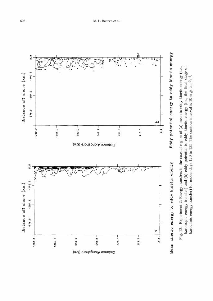
Meanders in the equatorward surface current formed by model day 135 in the equatorwardend of the model domain, as seen in the velocity and temperature plots (Figs. 11(c) and 12(b),respectively). The results for the instability analysis (Fig. 13) for the time period (i.e., days 120–135) during which the meanders developed, show that, although both types of instabilities arepresent in the coastal region of the model domain, barotropic instability (Fig. 13(a)) is dominantover baroclinic (Fig. 13(b)) instability in the equatorward end of the model domain.

By model day 180, the meanders begin to form cold core, cyclonic eddies as seen in thetemperature and velocity plots (Figs. 11(d) and 12(c), respectively), due to vertical and horizontalshear instabilities between the equatorward jet and the poleward undercurrent. By model day225, the meanders also begin to form warm, anticyclonic eddies, as seen in the temperature andvelocity plots (Fig. 11(d) and 12(e), respectively). Both the cyclonic and anticyclonic eddiesinitially appear to be about 100 km in diameter and extend about 200 km off the coast. As inExperiment 1, the eddies propagate farther offshore with speeds of ~5–10 km/day, and have timescales on the order of months. Unlike Experiment 1, as the eddies move offshore, they becomeembedded in the oceanic branch of the surface equatorward current, which veers further offshorewith time (see Figs. 11(e) and 11(f), for example).

At the end of the model year, these features are still discernible. Upwelling and filaments arestill present (Fig. 12(e)). The coastal branch of the equatorward surface current, the undercurrent,

Fig. 14. Experiment 2: Total (solid line), mean (dashed line), and eddy (dotted line) kinetic energy perunit time series for the upper layer over the entire domain for the first 900 days.


upwelling, meanders, filaments, and eddies are due to the predominantly equatorward windforcing. These features are similar to Experiment 1. Unlike Experiment 1, an offshore branch ofthe equatorward surface current is also generated. This feature originates in the vicinity of theSouth Pacific Subtropical High and its location of highest velocities migrates meridionally withthe location of the center of the South Pacific Subtropical High.

Longer experimental runs of three more years show that the system reaches a quasi-equilibrium of the annual cycle (Fig. 14) and that these features continue to be maintained (Fig.15). Note that the mean kinetic energy (Fig. 14) reaches a quasi-equilibrium of the annual cycle.This is expected, since the source for the mean kinetic energy, i.e., the wind forcing, is seasonal.Time averaging every 3 days from days 365–1085 of the meridional component of velocity isuseful for showing the permanent currents. The results (Fig. 15) show the presence of a coastalequatorward CPC, within ~100 km of the coast with speeds from 10–30 cm/s, which broadensoffshore in the equatorward end of the model domain; an offshore CPC centered ~300 kmoffshore with speeds of ~10 cm/s in the poleward end of the model domain; and a poleward PCUwithin ~50 km of the coast with speeds of ~1–5 cm/s. The location of the strongest velocities (~10cm/s) of the oceanic CPC seasonally migrates with the location of the center of the South PacificSubtropical High.

As in Experiment 1, the main contribution to the total kinetic energy is the eddy kineticenergy. The growth of eddy kinetic energy seen in Fig. 14 from ~days 100 to 500 is consistentwith the growth of eddies over the same time period (e.g., see Figs. 11(c)–(f)). Since the eddies,which have average velocities larger than the offshore CPC, are generated on the offshore side

Fig. 15. Experiment 2: Time-averaged meridional component of velocity at (a) the surface and (b) ~300m depth. The time averaging is every 3 days from days 365–1085. The contour interval is 10 cm/s in(a) and 2 cm/s in (b).


References:(1)Wooster and Reid (1963).(2)Tchernia (1980).(3)Fonseca (1989).(4)Codispoti et al. (1989).(5)Neshyba (1989).

Features Observation Experiment 1 Experiment 2

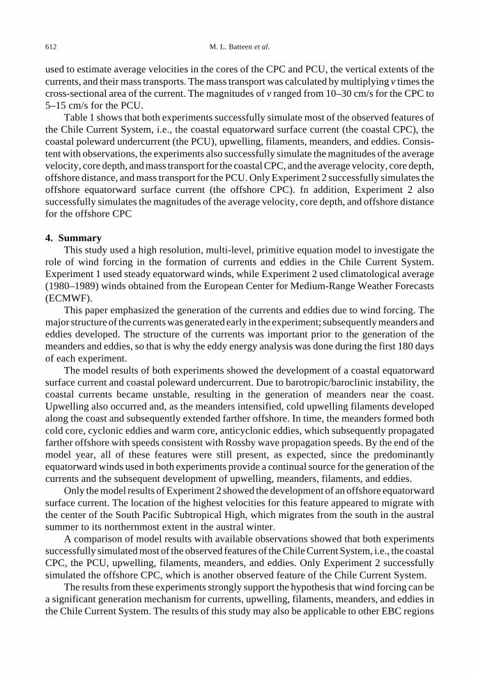
A. Coastal equatorward surface current (coastal Peru-Chile Current (CPC))1. Average velocity (cm/s) >10(1) 10–30 10–302. Core depth, vertical extent (m) Surface, <200(2) Surface, <150 Surface, <2503. Mass transport (10 6 m3/s) 19(1) 20 20

B. Offshore equatorward surface current (offshore CPC)1. Average velocity (cm/s) 10–15(2) not simulated 102. Core depth, vertical extent (m) Surface, <700(2) not simulated Surface, <250–4003. Offshore distance (km) >200(2) not simulated >200

C. Coastal poleward undercurrent (Peru-Chile Undercurrent (PCU))1. Average velocity (cm/s) 5–10(3),(4) 5–15 3–152. Core depth, vertical extent (m) 150–200,

<600(3)100–150, <600 150, <600

3. Offshore distance (km) <200(3) 50 75–1004. Mass transport (10 6 m3/s) 10(3) 10 10

D. Upwelling observed simulated simulated

E. Filaments: Offshore extent (km) 0 (100)(5) 0 (100) 0 (100)

F. Meander observed simulated simulated

G. Eddies: Core size (km) 0 (100)(5) 0 (100) 0 (100)

Table 1. Comparisons of model results with available observations.

of the coastal CPC and subsequently move slowly westward, they dominate most of the modeldomain throughout most of the model simulation time, resulting in the large contribution to thedomain-averaged eddy and total kinetic energies (Fig. 14).

3.3 Comparison of model results with observationsA comparison of model results with available observations was carried out to see if model

simulations of the currents and other features were consistent with the observed data for the ChileCurrent System. Table 1 highlights the primary features in the Chile Current System. It also liststhe specific characteristics (if available observations exist for them) for each feature along withthe corresponding model result for each experiment.

For the model results, meridional velocity (v) cross-sections, taken in the middle of themodel domain and averaged over 30-day periods (from days 360–900 of each experiment), were


used to estimate average velocities in the cores of the CPC and PCU, the vertical extents of thecurrents, and their mass transports. The mass transport was calculated by multiplying v times thecross-sectional area of the current. The magnitudes of v ranged from 10–30 cm/s for the CPC to5–15 cm/s for the PCU.

Table 1 shows that both experiments successfully simulate most of the observed features ofthe Chile Current System, i.e., the coastal equatorward surface current (the coastal CPC), thecoastal poleward undercurrent (the PCU), upwelling, filaments, meanders, and eddies. Consis-tent with observations, the experiments also successfully simulate the magnitudes of the averagevelocity, core depth, and mass transport for the coastal CPC, and the average velocity, core depth,offshore distance, and mass transport for the PCU. Only Experiment 2 successfully simulates theoffshore equatorward surface current (the offshore CPC). fn addition, Experiment 2 alsosuccessfully simulates the magnitudes of the average velocity, core depth, and offshore distancefor the offshore CPC

4. SummaryThis study used a high resolution, multi-level, primitive equation model to investigate the

role of wind forcing in the formation of currents and eddies in the Chile Current System.Experiment 1 used steady equatorward winds, while Experiment 2 used climatological average(1980–1989) winds obtained from the European Center for Medium-Range Weather Forecasts(ECMWF).

This paper emphasized the generation of the currents and eddies due to wind forcing. Themajor structure of the currents was generated early in the experiment; subsequently meanders andeddies developed. The structure of the currents was important prior to the generation of themeanders and eddies, so that is why the eddy energy analysis was done during the first 180 daysof each experiment.

The model results of both experiments showed the development of a coastal equatorwardsurface current and coastal poleward undercurrent. Due to barotropic/baroclinic instability, thecoastal currents became unstable, resulting in the generation of meanders near the coast.Upwelling also occurred and, as the meanders intensified, cold upwelling filaments developedalong the coast and subsequently extended farther offshore. In time, the meanders formed bothcold core, cyclonic eddies and warm core, anticyclonic eddies, which subsequently propagatedfarther offshore with speeds consistent with Rossby wave propagation speeds. By the end of themodel year, all of these features were still present, as expected, since the predominantlyequatorward winds used in both experiments provide a continual source for the generation of thecurrents and the subsequent development of upwelling, meanders, filaments, and eddies.

Only the model results of Experiment 2 showed the development of an offshore equatorwardsurface current. The location of the highest velocities for this feature appeared to migrate withthe center of the South Pacific Subtropical High, which migrates from the south in the australsummer to its northernmost extent in the austral winter.

A comparison of model results with available observations showed that both experimentssuccessfully simulated most of the observed features of the Chile Current System, i.e., the coastalCPC, the PCU, upwelling, filaments, meanders, and eddies. Only Experiment 2 successfullysimulated the offshore CPC, which is another observed feature of the Chile Current System.

The results from these experiments strongly support the hypothesis that wind forcing can bea significant generation mechanism for currents, upwelling, filaments, meanders, and eddies inthe Chile Current System. The results of this study may also be applicable to other EBC regions


which have predominantly equatorward wind forcing, such as the central and southern regionsof the California Current System.

AcknowledgementsThis work was done in the Department of Oceanography at the Naval Postgraduate School

under the support of the Office of Naval Research and the National Science Foundation. We wishto thank Dr. Yoshiteru Kitamura and the reviewers for valuable comments on how to clarify thetext.

ReferencesArakawa, A. and V. R. Lamb (1977): Computational design of the basic dynamical process of the UCLA general

circulation model. p. 173–265. In Methods in Computational Physics, Vol. 17, ed. by J. Chang, Academic Press,New York.

Bakun, A. and C. S. Nelson (1991): The seasonal cycle of windstress curl in subtropical eastern boundary currentregions. J. Phys. Oceanogr., 21, 1815–1834.

Batteen, M. L. and Y.-J. Han (1981): On the computational noise of finite-difference schemes used in ocean models.Tellus, 33, 387–396.

Batteen, M. L., R. L. Haney, T. A. Tielking and P. G. Renaud (1989): Numerical study of wind forcing of eddiesand jets in the California Current System. J. Mar. Res., 47, 493–523.

Batteen, M. L., M. J. Rutherford and E. J. Bayler (1992): A numerical study of wind- and thermal-forcing effectson the ocean circulation off Western Australia. J. Phys. Oceanogr., 22, 1406–1433.

Camerlengo, A. L. and J. J. O’Brien (1980): Open boundary conditions in rotating fluids. J. Comput. Phys., 35, 12–35.

Carton, J. A. (1984): Coastal circulation caused by an isolated storm. J. Phys. Oceanogr., 14, 114–124.Carton, J. A. and S. G. H. Philander (1984): Coastal upwelling viewed as a stochastic phenomena. J. Phys. Oceanogr.,

14, 1499–1509.Codispoti, L. A., R. T. Barber and G. E. Friederich (1989): Do nitrogen transformations in the poleward undercurrent

off Peru and Chile have a globally significant influence? p. 281–310. In Poleward Flows along Eastern OceanBoundaries, ed. by S. J. Neshyba, C. N. K. Mooers, R. L. Smith and R. T. Barber, Springer-Verlag, New York.

Fonseca, T. R. (1989): An overview of the poleward undercurrent and upwelling along the Chilean Coast. p. 203–218. In Poleward Flows along Eastern Ocean Boundaries, ed. by S. J. Neshyba, C. N. K. Mooers, R. L. Smithand R. T. Barber, Springer-Verlag, New York.

Gunther, E. R. (1936): A report on oceanographical investigations in the Peru Coastal Current. Discovery Rep., 13,107–276.

Han, Y.-J. (1975): Numerical simulation of mesoscale eddies. Ph.D. Thesis, University of California, Los Angeles,154 pp.

Haney, R. L. (1974): A numerical study of the response of an idealized ocean to large-scale surface heat andmomentum flux. J. Phys. Oceanogr., 4, 145–167.

Holland, W. R. (1978): The role of mesoscale eddies in the general circulation of the ocean—Numerical experimentsusing a wind-driven quasigeostrophic model. J. Phys. Oceanogr., 8, 363–392.

Holland, W. R. and M. L. Batteen (1986): The parameterization of subgrid scale heat diffusion in eddy-resolvedocean circulation models. J. Phys. Oceanogr., 16, 200–206.

Levitus, S. (1982): Climatological atlas of the world ocean. NOAA Prof. Paper 13, U.S. Dept. of Commerce,Washington, D.C., 173 pp.

McCreary, J. P. (1981): A linear stratified ocean model of the coastal undercurrent. Phil. Trans. R. Soc. Lond. A, 302,385–413.

McCreary, J. P., P. K. Kundu and S. Y. Chao (1987): On the dynamics of the California Current System. J. Mar. Res.,45, 1–32.

Mooers, C. N. K. and A. R. Robinson (1984): Turbulent jets and eddies in the California Current and inferred cross-shore transports. Science, 223, 51–53.

Nelson, C. S. (1977): Wind stress and wind stress curl over the California Current. NOAA Tech. Rep. NMFS SSFR-714, U.S. Dept. Commerce, 87 pp.

Neshyba, S. (1989): Oceanography: Perspectives on a Fluid Earth. John Wiley and Sons, Inc., New York, 506 pp.


Pedlosky, J. (1974): Longshore currents, upwelling and bottom topography. J. Phys. Oceanogr., 4, 214–226.Philander, S. G. H. and J. H. Yoon (1982): Eastern boundary currents and coastal upwelling. J. Phys. Oceanogr.,

12, 862–879.Semtner, A. J. and Y. Mintz (1977): Numerical simulation of the Gulf Stream and midocean eddies. J. Phys. Oceanogr.,

7, 208–230.Tchernia, P. (1980): Descriptive Regional Oceanography. Pergamon Press, New York, 253 pp.Trenberth, K. E., W. G. Large and J. G. Olson (1990): The mean annual cycle in global ocean wind stress. J. Phys.

Oceanogr., 20, 1742–1760.Weatherly, G. L. (1972): A study of the bottom boundary layer of the Florida Current. J. Phys. Oceanogr., 2, 54–

72.Wooster, W. S. and M. Gilmartin (1961): The Peru-Chile Undercurrent. J. Mar. Res., 19, 97–122.Wooster, W. S. and J. L. Reid (1963): Eastern boundary currents. p. 253–280. In The Sea, Vol. 2, ed. by M. N. Hill,

Wiley Interscience, New York.Zeigler, J. M., W. D. Athearn and H. Small (1957): Profiles across the Peru-Chile Trench. Deep-Sea Res., 4, 238–

249.

a numerical study of the effects of wind forcing on the...

Documents