a parameterization of size resolved below cloud scavenging of

Atmos. Chem. Phys., 6, 3363–3375, 2006www.atmos-chem-phys.net/6/3363/2006/© Author(s) 2006. This work is licensedunder a Creative Commons License.

AtmosphericChemistry

and Physics

A parameterization of size resolved below cloud scavenging ofaerosols by rain

J. S. Henzing1, D. J. L. Olivi e2, and P. F. J. van Velthoven1

1Royal Netherlands Meteorological Institute KNMI, De Bilt, The Netherlands2Meteo France, CNRM, Toulouse, France

Received: 28 October 2005 – Published in Atmos. Chem. Phys. Discuss.: 20 February 2006Revised: 19 June 2006 – Accepted: 29 June 2006 – Published: 14 August 2006

Abstract. A size dependent parameterization for the re-moval of aerosol particles by falling rain droplets is devel-oped. Scavenging coefficients are calculated explicitly as afunction of aerosol particle size and precipitation intensityincluding the full interaction of rain droplet size distribu-tion and aerosol particles. The actual parameterization is asimple and accurate three-parameter fit through these pre-calculated scavenging coefficients. The parameterization isapplied in the global chemistry transport model TM4 and theimportance of below-cloud scavenging relative to other re-moval mechanisms is investigated for sea salt aerosol. For afull year run (year 2000), we find that below-cloud scaveng-ing accounts for 12% of the total removal of super-micronaerosol. At mid-latitudes of both hemispheres the fractionalcontribution of below-cloud scavenging to the total removalof super-micron sea salt is about 30% with regional maximaexceeding 50%. Below-cloud scavenging reduces the globalaverage super-micron aerosol lifetime from 2.47 to 2.16 daysin our simulations. Despite large uncertainties in precipita-tion, relative humidity, and water uptake by aerosol particles,we conclude that below cloud scavenging is likely an impor-tant sink for super-micron sized sea salt aerosol particles thatneeds to be included in size-resolved aerosol models.

1 Introduction

Aerosol removal processes remain an important source ofuncertainty in global aerosol transport models (Rasch et al.,2000). Recent aerosol model intercomparisons such as Aero-Com (AeroCom, 2005; Textor et al., 2006) show significantdifferences in modeled atmospheric aerosol concentrationsthat might be due to differences in the model representationsof wet removal of aerosols. Aerosol particles are very effi-

Correspondence to:P. F. J. van Velthoven([email protected])

ciently removed from the atmosphere by in-cloud and below-cloud scavenging processes. For accumulation mode aerosolthe in-cloud removal, governed by aerosols serving as cloudcondensation nuclei or ice nuclei and subsequent removal byprecipitation, is by far the most efficient atmospheric sink.However, very small particles are more easily scavenged byrain droplets because they are rapidly transferred into fallingdroplets as their Brownian motion exceeds the rain dropletfall velocity. Coarse particles are also more easily scavengedthan accumulation mode aerosols because of their size andinertness (Slinn, 1984; Pruppacher and Klett, 1997). Us-ing explicit calculations of the efficiency of collision be-tween size distributions of raindrops and aerosol particles,Andronache (2004) and Zhang et al. (2004) showed that evenweak precipitation can remove 50–80% of the below-cloudaerosol in both number and mass.

On-line calculation of the full interaction between thesize spectra of aerosol particles and precipitation, in orderto obtain below-cloud scavenging parameters in large-scaleaerosol models is (yet) unrealistic due to the large compu-tational time involved. Therefore, studies often describe thesize-resolved aerosol load as a diagnostic variable (Collinset al., 2001) or they confine themselves to precipitation freeepisodes so that wet removal can be neglected (Schulz et al.,1998; Vignati et al., 2001). Studies that do include size re-solved below-cloud scavenging use constant scavenging pa-rameters for aerosols that are confined to size-modes (Stieret al., 2005), use simple bulk parameterizations based onprecipitation intensities (Balkanski, et al., 1993) or use ap-proximate expressions for the scavenging rate based on e.g.mean rain droplet size (Gong et al., 2003a). Tost et al. (2006)actually calculate the size-dependent scavenging coefficientsonline, but they assume a monodisperse (rain) droplet spec-trum. However, Andronache (2003) showed that the colli-sion efficiency and thus the scavenging coefficients depen-dent strongly on the raindrop size.

Published by Copernicus GmbH on behalf of the European Geosciences Union.

3364 J. S. Henzing et al.: Size resolved below cloud scavenging of aerosols

The purpose of this study is the development of a pa-rameterization that provides the scavenging coefficient as afunction of aerosol particle size and precipitation intensity.The parameterization consists of a simple fit through below-cloud scavenging coefficients calculated at high resolution.The calculations are based on the concept of efficiency ofcollision between polydisperse aerosol and raindrop distri-butions (Slinn, 1983; Pruppacher and Klett, 1997; Seinfeldand Pandis, 1998). This method is widely applied and hasbeen evaluated (e.g. Mircea et al., 2000; Andronache, 2003,2004; Zhang, 2004). The parameterization will be appliedto size resolved sea salt aerosol in the global chemistry trans-port model TM4. The importance of below-cloud scavengingrelative to other removal mechanisms will be discussed andthe impact on the overall sea salt aerosol lifetime will be in-vestigated.

2 Below cloud scavenging coefficient

2.1 Explicit calculation

A rain droplet with radiusR, sweeps per unit of time approx-imately the volume of a cylinder equal toπ(R+r)2(Ut−ut ),whereUt is the droplet speed of fall,ut the aerosol particlespeed of fall, andr the aerosol particle radius. However, afalling droplet also perturbs the neighboring air and createsa flow-field around the droplet. Therefore, the actual vol-ume swept by the falling droplet depends on the ability ofthe aerosol particle to adjust to the flow streamlines. Thesolution of this fluid mechanics problem is often expressedin terms of the collision efficiencyE(R, r), which is de-fined as the fraction of aerosol particles contained within thesweep-cylinder-volume that actually collides with the fallingdroplets. We can assume that the aerosol particle speed of fallis small compared to the rain droplet speed of fall and that theaerosol particle radius is small compared to the rain dropletradius. The differential scavenging coefficientβ, which is thefractional amount (number, mass etc.) of aerosol removed byprecipitation per unit time for a fixed aerosol particle radius,is then given by (Engelmann, 1968):

β (r) =

∫∞

0πR2Ut (R) εE (R, r) N (R) dR , (1)

where N (R)dR is the number of rain droplets with radiibetweenR andR+dR per unit volume andε is the reten-tion efficiency that determines whether the collision betweendroplet and particle is effective. Below it is explained howthe various terms that are necessary to perform the integra-tion of Eq. (1) can be calculated.

2.1.1 Rain droplet velocity

In our calculations we will assume that rain droplets alwaysfall at their terminal velocities. We base our rain droplet ter-minal velocity on an empirical representation given by Atlas

et al. (1973) but forR<0.3 mm we force the droplet veloc-ity smoothly to zero using a linear fit to measurements ofGunn and Kinzer (1949) as proposed by Matzler (2002). Thepressure-independent droplet terminal velocity [m s−1] overthe whole range is then given by:

Ut (R)=

0 ; R ≤ 0.015 mm4.323(R−0.015) ; 0.015≤R≤0.3 mm9.65−10.3 exp(−0.3R) ; R>0.3 mm

(2)

2.1.2 Rain droplet size distribution

We base our rain droplet size distribution on a gamma func-tion fit of De Wolf (2001) to the pioneering size distribu-tion measurements of Laws and Parsons (1943). We choosethe gamma fit instead of the more traditional exponentialfunction fit (Marshall and Palmer, 1948), because it repre-sents the size distribution over the whole particle size spec-trum whereas the exponential fits overestimate the numberof droplets at the small end of the particle size spectrum.Making use of the droplet terminal velocity (Eq. 2), Matzler(2002) properly normalized the De Wolf size distribution.Normalization assures that the precipitation intensity com-puted from the droplet size distribution (Eqs. 3a, b) and theiraccessory speed of fall (Eq. 2) is consistent with the rain rateinput variable,P (Eqs. 3a, b). The empirical expression forthe number of drops with drop radii betweenR andR+dR,per unit volume of air, as a function of rain rateP is given:

N (R, P ) = norm· 1.98 · 10−5P −0.384R2.93

exp[−

(5.38P −0.186

· R)]

, (3a)

where

norm= 1.047− 0.0436· ln P + 0.00734· (ln P)2 . (3b)

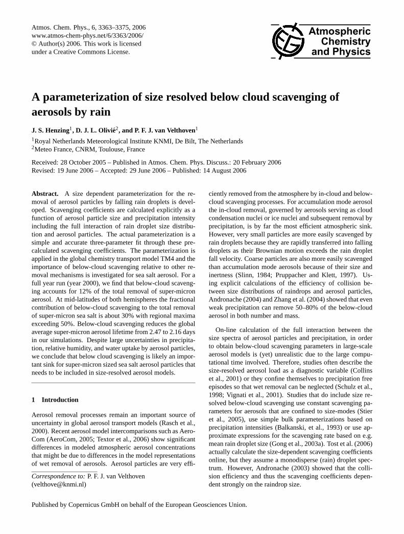
The adopted rain droplet size distribution (“De Wolf”) isshown in Fig. 1 for a precipitation intensity of 5 mm h−1.

2.1.3 Raindrop-aerosol collection efficiency

The collision efficiency,E(R, r) expresses the probabilitythat an aerosol particle that resides in the geometrical cylin-der swept in a certain time interval by the cross-section of afalling rain droplet, actually collides with the droplet. Weassume that every collision is efficient: the sticking effi-ciency or retention,ε, is unity (Pruppacher and Klett, 1997),in contrast to particle-particle collisions. The collection ef-ficiency, εE, is therefore equal to the collision efficiency.A value of εE=1 implies that all particles in the geomet-ric sweep-cylinder will be collected. In generalεE�1, ex-cept for charged particles and very small Brownian particles(e.g. nanometer-sized particles formed by homogeneous nu-cleation) that are both not considered in our study. Theo-retical solution of the Navier-Stokes equation for predictionof the collision efficiency for the general rain droplet-aerosol

Atmos. Chem. Phys., 6, 3363–3375, 2006 www.atmos-chem-phys.net/6/3363/2006/

J. S. Henzing et al.: Size resolved below cloud scavenging of aerosols 3365

0 1 2 3 4 5 6 7 8raindrop radius [mm]

10-4

10-3

10-2

10-1

100

101

102

103

104

105

N [m

-3 m

m-1

]

Marshall PalmerJoss DrizzleJoss ThunderstormDe Wolf

Fig. 1. The normalized rain droplet size distribution (precipita-tion intensity 5 mm h−1), as used in our study (De Wolf) togetherwith three other widely used size distributions (for a discussion seeSect. 5).

interaction case is a difficult undertaking due to the compli-cated induced flow patterns around the falling drop. Insteadof exactly solving the Navier-Stokes equations we use an al-ternative expression forE that is based on dimensional anal-ysis and experimental data (Slinn, 1984). The reader is re-ferred to Seinfeld and Pandis (1998, their Sect. 20.3.1) for afull description of the appliedE.

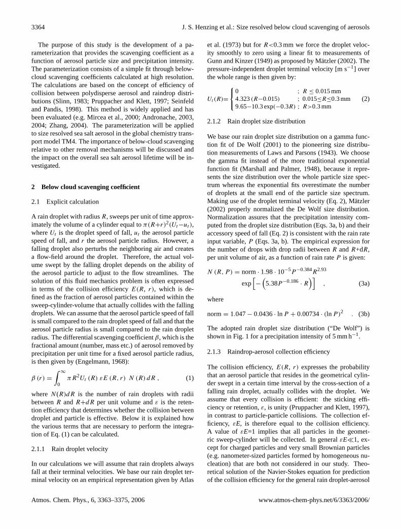
The scavenging coefficientβ as a function of aerosol par-ticle radius and precipitation intensity is explicitly calculatedusing Eq. (1) and is shown in Fig. 2. The dark blue/black areain the figure clearly identifies the well-known Greenfield gap,where aerosols are not effectively removed by falling raindroplets. The strong increase in the scavenging coefficient atparticle sizes of about 2µm marks the transition to the sizeregion where inertial impaction becomes the dominant con-tributor to the collection efficiency.

2.2 Parameterization

To avoid the computationally expensive integration of Eq. (1)in our chemistry transport model, we fit an analytical func-tion through the pre-calculated values of the scavenging coef-ficient for every aerosol particle radius (1000 log-equidistantincrements per order of magnitude increase in particle radius)(Fig. 2). A function of the form

β (P ) = A0

(eA1P

A2− 1

), (4)

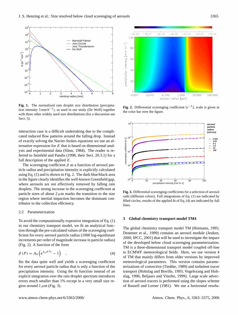
fits the data quite well and yields a scavenging coefficientfor every aerosol particle radius that is only a function of theprecipitation intensity. Using the fit function instead of anexplicit integration over the rain droplet spectrum introduceserrors much smaller than 1% except in a very small size re-gion around 1µm (Fig. 3).

Fig. 2. Differential scavenging coefficient [s−1], scale is given inthe color bar over the figure.

0 20 40 60 80 100precipitation intensity [mm hr-1]

10-8

10-6

10-4

10-2

100

scav

engi

ng c

oeffi

cien

t [s-

1] 0.0010.010.11.010100

aerosolparticleradius[micron]

Fig. 3. Differential scavenging coefficients for a selection of aerosolradii (different colors). Full integrations of Eq. (1) are indicated byfilled circles, results of the applied fit of Eq. (4) are indicated by fulllines.

3 Global chemistry transport model TM4

The global chemistry transport model TM (Heimann, 1995;Dentener et al., 1999) contains an aerosol module (Jeuken,2000; IPCC, 2001) that will be used to investigate the impactof the developed below cloud scavenging parameterization.TM is a three-dimensional transport model coupled off-lineto ECMWF meteorological fields. Here, we use version 4of TM that mainly differs from older versions by improvedmeteorological parameters. This version contains parame-terizations of convective (Tiedtke, 1989) and turbulent tracertransport (Holtslag and Boville, 1993; Vogelezang and Holt-slag, 1996; Beljaars and Viterbo, 1999). Large scale advec-tion of aerosol tracers is performed using the slopes schemeof Russell and Lerner (1981). We use a horizontal resolu-

www.atmos-chem-phys.net/6/3363/2006/ Atmos. Chem. Phys., 6, 3363–3375, 2006


tion of 6◦ in longitude and 4◦ in latitude. In the verticalthe total number of hybridσ -pressure levels (Simmons andBurridge, 1981) has been reduced from 60 (ECMWF) to 25(TM4) by merging selected layers, mostly in the stratosphere.The scavenging parameterization will be evaluated for seasalt whose parameterization in the model was recently up-dated, as described below.

3.1 Sea salt source function

A source for sea salt aerosol particles (Gong, 2003b) that isbased on the source function given by Monahan et al. (1986)has been included in the model. This source function, whichis a function of the wind speed at 10-m height (U10), providesthe number of particles emitted in a certain size range per unittime and per unit sea surface:

dF

dr= 1.373u3.41

10 r−A(1 + 0.057r3.45

)· 101.607e−B2

, (5)

where r is the particle radius at relative humidity 80%,A=4.7(1+2r) −0.017r−1.44

, B=(0.433−logr)/0.433, and2in A is an adjustable parameter that controls the shape ofthe sub-micron size distribution. Here2=30 as in Gong etal. (2003b). In our model the series of physical transport pro-cesses on sea salt aerosol are most conveniently formulatedin terms of the dry part of the aerosol particles. Therefore,we have translated the source function, which is valid at 80%relative humidity (Monahan et al., 1983), in a dry particlesource function using the size dependence of sea salt aerosolas a function of relative humidity given by Gerber (1985):

r =

[C1r

C2d

C3rC4d − logRH

+ r3d

]1/3, (6)

where rd is the dry particle radius [cm], RHthe relative humidity [%], and C1(=0.7664),C2(=3.079),C3(=2.5730·10−11),C4(=−1.424) are pa-rameters for different types of aerosol particles (valuesbetween brackets are valid for sea salt. To solve the sizedistribution both in number and mass it is sufficient to use 12log-equidistant sectional bins (Gong et al., 2003a). Our 12bins cover the dry radius spectrum from 0.03µm to 10.0µm.Offline, we have calculated the mass emission [kg sea saltper second and per unit sea surface] in every bin of 1 m s−1

wind speed, from which the actual emission is obtained bymultiplication with U3.41

10 (Eq. 5). In the model, aerosolparticles are assumed to be in a stable equilibrium size withrespect to ambient relative humidity. The actual size ofsea salt aerosol, which is used to calculate the below-cloudscavenging, is related to their dry size by the relationship ofGerber (1985).

3.2 Aerosol sinks

3.2.1 Large scale cloud systems

The change in aerosol mass mixing ratioµ due to thescavenging by precipitation can be obtained by applyingan equivalent fractional loss termf that accounts for thesubgrid-scale patchiness of precipitation (Walton et al.,1988):

µ (t + 1t) = µ (t) · f ≡ µ (t) · (V1f1 + V2f2 + V3) , (7)

where indicesi=1–3 represent respectively the region insideprecipitating clouds, the region below precipitating clouds,and cloud free regions,Vi is the fraction of the grid cell oc-cupied by region of typei, andfi=exp[−βi1t ] whereβi isthe scavenging coefficient for region of typei and1t is thetime between two calls of the removal scheme. VolumeV1is simply the cloud fraction. VolumeV2 (below precipitatingcloud) is the fraction of the cell that is cloud free but over-cast (using the maximum overlap assumption). VolumeV3 iscloud free and there are no clouds in overlying layers. Theassumption of an equivalent fractional loss term implicitlyassumes that aerosols are uniformly distributed within eachgrid cell. We observed that when this scheme is applied athigh temporal resolution, aerosol is removed too efficiently.The explanation is that it is implicitly assumed that aerosolis mixed from aerosol rich (cloud free) regions into aerosolpoor (precipitating) regions after every removal step whereasin reality the precipitating systems still affect, for a large part,the same aerosol containing air mass. To overcome this prob-lem, we effectively postpone the mixing. To do so we defineda no-mixing-timescale,1tno−mix=N ·1t , whereN is an ad-justable parameter, and we reformulated the equivalent frac-tional loss term that then becomes a function of the numberof calls,n, of the removal scheme since the last mixing in-stant:

f ∗ (n) =V1f

n1 + V2f

n2 + V3

V1fn−11 + V2f

n−12 + V3

. (8)

If we neglect all other processes but the removal scheme wefind for n=N :

µ (t + N1t) = f ∗ (N) · µ (t + (N − 1) 1t) , (9)

µ (t + N1t) = f ∗ (N)·f ∗ (N − 1)·.....·f ∗ (1)·µ (t) , (10)

µ (t + N1t) =

(V1f

N1 + V2f

N2 + V3

)· µ (t) , (11)

which equals the mixing ratio that would be obtained if airmasses and precipitating clouds would be kept fixed at theirrelative positions for a time period1tno−mix. A convenientassumption for the no-mixing-timescale is the time betweensuccessive updates of the meteorological input, which is sixhours in our model.



Below cloud scavenging

The differential scavenging coefficient,β(r), obtainedup to now, corresponds to a given, fixed aerosol particleradius. To derive an integral scavenging coefficient that isvalid for the total aerosol mass contained within a certainsize bin, Eq. (1) has to be integrated over the aerosol particlemass distribution (Dana and Hales, 1976):

β (rs) =

∫ rr

rl

β (r) fmass(r) dr , (12)

where rl and rr are the left and right borders of the sizebin, fmass(r)dr is the mass probability distribution func-tion (pdf), and subscript “s” indicates that the scavengingcoefficient is obtained by integration over the aerosol massspectrum that is contained in the size bin. Within a sizebin the mass-pdf is unknown. As a first approximation wesimply assume that the mass is equally distributed withina bin. The resolution with respect to aerosol radius of theparameterized differential scavenging coefficients is chosensuch that the scavenging coefficient at the exact radiusof the (wet) size bin borders can be obtained by linearinterpolation of adjacent scavenging coefficients withoutintroducing additional errors (�1%). A table with theselected coefficientsA0−A2 that are used to calculate thedifferential scavenging coefficients with Eq. (4) are availableathttp://www.knmi.nl/∼velthove/wetdeposition.

In-cloud scavenging

The in-cloud scavenging coefficient is determined bytwo sequential steps: In the first step cloudwater is formedfrom water vapor. Here, we neglect the existence of inter-stitial aerosol and thus assume that all aerosol particles actas condensation nuclei. All aerosol is therefore included inthe cloudwater that is formed. In the second step precip-itation is formed from the aerosol-containing cloudwater.The precipitation formation rate thus fully determines theremoval process (Roelofs and Lelieveld, 1995). The actualscavenging coefficient is the fraction of cloud water that isconverted into rain water per unit of time.

3.2.2 Dry deposition

Dry deposition, the amount of material deposited to a unitsurface area per unit time,F , is calculated as:

F = −vdC , (13)

where the constant of proportionality,vd , with units of lengthper unit time is the deposition velocity. The dry depositionvelocity of aerosol particles is a function of turbulent state ofthe atmosphere and of particle aerodynamic size. Based on

theoretical considerations Slinn and Slinn (1980) derived anexpression for the deposition velocity,

vd =

(va + vg

) (vb + vg

)(va + vb + vg

) , (14)

whereva , vb, andvg are velocities. Velocityva , representsthe rate of material transport by turbulence from a referenceheight in the free troposphere to a layer of stagnant air justabove and adjacent to the surface (quasi-laminar sublayer).In our modelva=1/ra , wherera is the aerodynamic resis-tance that is calculated and stored at ECMWF. Analogously,the transfer velocity in the quasi-laminar sublayer is writtenvb=1/rb, whererb is the resistance to transfer which dependsupon Brownian diffusion accounted for by the Schmidt num-ber (Sc), and upon inertial impaction, accounted for by theStokes number (St) (Slinn, 1982):

rb =1

u∗

(Sc

−2/3 + 10−3/St

) , (15)

where u∗ is the friction velocity, Sc=ν/D, where ν is

the kinematic viscosity andD the Brownian diffusion andSt=vgu

2∗

/gν, whereg is the gravitational acceleration. The

gravitational settling velocity is given by Stokes Law,

vg =4ρpr2

pg

18µ, (16)

whereρp is the density of the particle,rp is the particle ra-dius,µ is the viscosity of air.

3.2.3 Convective cloud systems

The scavenging by convective precipitation is proportional tothe mass flux entrained in convective clouds, as in Balkanskiet al. (1993) and Guelle et al. (1998). We apply rather arbi-trary scavenging efficiencies of 50% for shallow convectionup to 700 hPa and of 80% for deep convection. Furthermore,we include an exponential scaling factor to avoid removal inthe case of relatively dry updrafts. In the absence of pre-cipitation there is no removal, for a precipitation intensityof 1 mm/h the scaling is 0.85, and for higher intensities thescaling rapidly goes to 1 (no scaling).

4 Results

4.1 Emission, load, and lifetime

Applying our model with the newly implemented sea saltsource function (Gong, 2003b), we find for the year 2000a total sea salt mass emission of 2440 Tg for particles withdry radii between 0.03 and 10µm. This value falls wellwithin the range of estimates reported in the literature (1000to 3000 Tg/yr, Erickson and Duce, 1988; 5900 Tg/yr, Tegenet al., 1997) and can be compared to the current best estimate


http://www.knmi.nl/~velthove/wet_deposition


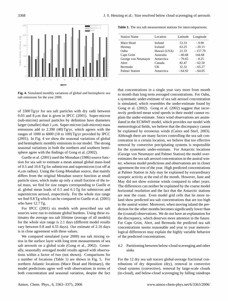
Fig. 4. Simulated monthly variations of global and hemispheric seasalt emissions for the year 2000.

of 3300 Tg/yr for sea salt particles with dry radii between0.03 and 8µm that is given in IPCC (2001). Super-micron(sub-micron) aerosol particles by definition have diameterslarger (smaller) than 1µm. Super-micron (sub-micron) massemissions add to 2.390 (48) Tg/yr, which agrees with theranges of 1000 to 6000 (18 to 100) Tg/yr provided by IPCC(2001). In Fig. 4 we show the seasonal variations of globaland hemispheric monthly emissions in our model. The strongseasonal variations in both the northern and southern hemi-sphere agree with the findings of Gong et al. (2002).

Guelle et al. (2001) used the Monahan (1986) source func-tion for sea salt to estimate a mean annual global mass-loadof 0.5 and 10.6 Tg for submicron and supermicron (cut off at4µm radius). Using the Gong-Monahan source, that mainlydiffers from the original Monahan source function at smallparticle sizes, which make up only a small fraction of the to-tal mass, we find for size ranges corresponding to Guelle etal. global mean loads of 0.5 and 6.1 Tg for submicron andsupermicron aerosol, respectively. For the whole size rangewe find 9.8 Tg which can be compared to Guelle et al. (2001)who have 12.7 Tg.

For IPCC (2001) six models with prescribed sea saltsources were run to estimate global burdens. Using these es-timates the average sea salt lifetime (average of all models)for the whole size range is 2.1 days (different model resultsvary between 0.8 and 4.55 days). Our estimate of 2.16 daysis in close agreement with these values.

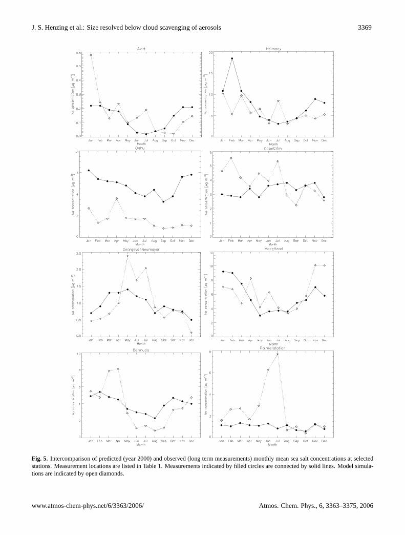
We compared simulated (year 2000) sea salt mixing ra-tios in the surface layer with long term measurements of seasalt aerosols on a global scale (Gong et al., 2002). Gener-ally, seasonally averaged model results agreed with observa-tions within a factor of two (not shown). Comparisons fora number of locations (Table 1) are shown in Fig. 5. Fornorthern Atlantic locations (Mace Head and Heimaey), themodel predictions agree well with observations in terms ofboth concentration and seasonal variation, despite the fact

Table 1. The sea salt measurement stations for intercomparisons.

Station Name Location Latitude Longitude

Mace Head Ireland 53.33 −9.90Heimay Iceland 63.25 −20.15Oahu Hawaii (USA) 21.33 −157.70Cape Grim Australia −40.68 144.68George von Neumayer Antarctica −70.65 −8.25Alert Canada 82.47 −62.50Bermuda UK 32.32 −65.27Palmer Station Antarctica −64.92 −64.05

that concentrations in a single year vary more from monthto month than long term averaged concentrations. For Oahu,a systematic under-estimate of sea salt aerosol concentrationis simulated, which resembles the under-estimate found byGong et al. (2002). Gong et al. (2002) suggest that incor-rectly predicted mean wind speeds in their model cannot ex-plain the under-estimate. Since wind observations are assim-ilated in the ECMWF model, which provides our model withmeteorological fields, we believe that the discrepancy cannotbe explained by erroneous winds (Caires and Sterl, 2003).Although there are many factors controlling the sea salt con-centration in a certain location, we believe that too effectiveremoval by convective precipitating systems is responsiblefor the systematic under-estimate. For Antarctic locations(George von Neumayer and Palmer Station) the model over-estimates the sea salt aerosol concentration in the austral win-ter, whereas model predictions and observations are in closeragreement the rest of the year. High predicted concentrationsat Palmer Station in July may be explained by extraordinarysynoptic activity at the end of the month. However, June andMay did not show extreme winds compared to other years.The differences can neither be explained by the coarse modelhorizontal resolution and the fact that the Antarctic stationsare near the coast. Even model grid cells that lie more in-land show predicted sea salt concentrations that are too highin the austral winter. Moreover, when moving inland the pre-diction for the other months becomes significantly lower thanthe (coastal) observations. We do not have an explanation forthe discrepancy, which deserves more attention in the future.For Cape Grim, Alert, and Bermuda the predicted sea saltconcentrations seems reasonable and year to year meteoro-logical differences may explain the highly variable behaviorof the predicted concentrations.

4.2 Partitioning between below-cloud scavenging and othersinks

For the 12 dry sea salt tracers global-average fractional con-tributions of dry deposition (dry), removal in convectivecloud systems (convective), removal by large-scale clouds(in-cloud), and below-cloud scavenging by falling raindrops



Fig. 5. Intercomparison of predicted (year 2000) and observed (long term measurements) monthly mean sea salt concentrations at selectedstations. Measurement locations are listed in Table 1. Measurements indicated by filled circles are connected by solid lines. Model simula-tions are indicated by open diamonds.



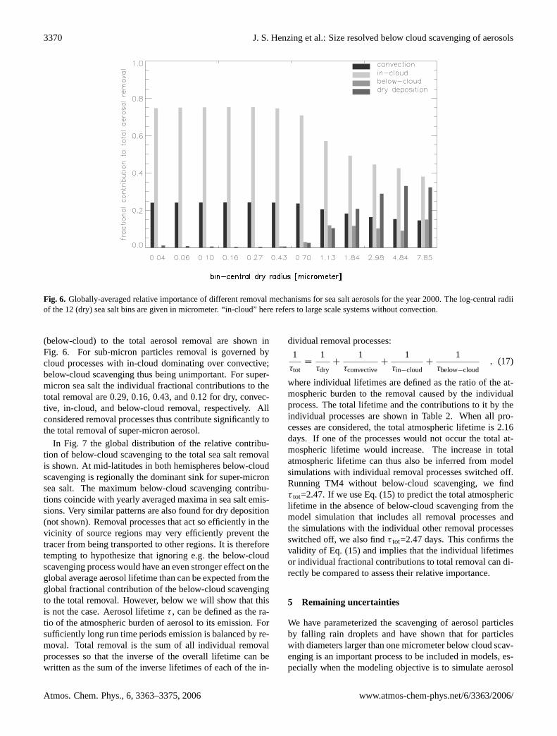
Fig. 6. Globally-averaged relative importance of different removal mechanisms for sea salt aerosols for the year 2000. The log-central radiiof the 12 (dry) sea salt bins are given in micrometer. “in-cloud” here refers to large scale systems without convection.

(below-cloud) to the total aerosol removal are shown inFig. 6. For sub-micron particles removal is governed bycloud processes with in-cloud dominating over convective;below-cloud scavenging thus being unimportant. For super-micron sea salt the individual fractional contributions to thetotal removal are 0.29, 0.16, 0.43, and 0.12 for dry, convec-tive, in-cloud, and below-cloud removal, respectively. Allconsidered removal processes thus contribute significantly tothe total removal of super-micron aerosol.

In Fig. 7 the global distribution of the relative contribu-tion of below-cloud scavenging to the total sea salt removalis shown. At mid-latitudes in both hemispheres below-cloudscavenging is regionally the dominant sink for super-micronsea salt. The maximum below-cloud scavenging contribu-tions coincide with yearly averaged maxima in sea salt emis-sions. Very similar patterns are also found for dry deposition(not shown). Removal processes that act so efficiently in thevicinity of source regions may very efficiently prevent thetracer from being transported to other regions. It is thereforetempting to hypothesize that ignoring e.g. the below-cloudscavenging process would have an even stronger effect on theglobal average aerosol lifetime than can be expected from theglobal fractional contribution of the below-cloud scavengingto the total removal. However, below we will show that thisis not the case. Aerosol lifetimeτ , can be defined as the ra-tio of the atmospheric burden of aerosol to its emission. Forsufficiently long run time periods emission is balanced by re-moval. Total removal is the sum of all individual removalprocesses so that the inverse of the overall lifetime can bewritten as the sum of the inverse lifetimes of each of the in-

dividual removal processes:

1

τtot=

1

τdry+

1

τconvective+

1

τin−cloud+

1

τbelow−cloud, (17)

where individual lifetimes are defined as the ratio of the at-mospheric burden to the removal caused by the individualprocess. The total lifetime and the contributions to it by theindividual processes are shown in Table 2. When all pro-cesses are considered, the total atmospheric lifetime is 2.16days. If one of the processes would not occur the total at-mospheric lifetime would increase. The increase in totalatmospheric lifetime can thus also be inferred from modelsimulations with individual removal processes switched off.Running TM4 without below-cloud scavenging, we findτ tot=2.47. If we use Eq. (15) to predict the total atmosphericlifetime in the absence of below-cloud scavenging from themodel simulation that includes all removal processes andthe simulations with the individual other removal processesswitched off, we also findτ tot=2.47 days. This confirms thevalidity of Eq. (15) and implies that the individual lifetimesor individual fractional contributions to total removal can di-rectly be compared to assess their relative importance.

5 Remaining uncertainties

We have parameterized the scavenging of aerosol particlesby falling rain droplets and have shown that for particleswith diameters larger than one micrometer below cloud scav-enging is an important process to be included in models, es-pecially when the modeling objective is to simulate aerosol



Table 2. Aerosol lifetimes,τ , for super-micron sea salt particles for a model simulation with and a simulation without the below-cloudscavenging parameterization. Subscripts “dry”, “below-cloud”, “in-cloud”, and “convective” refer to dry deposition, below cloud scavenging,scavenging in large scale clouds, and scavenging by convective clouds, respectively.

All Removal processes No below-cloud scavengingProcess Lifetime Fractional contribution Lifetime Fractional contribution

total removal total removal

Dry 7.43 0.29 7.77 0.32Below-cloud 17.43 0.12 – –In-cloud 5.07 0.43 4.85 0.51Convective 13.64 0.16 14.38 0.17Total 2.16 1.00 2.47 1.00

Fig. 7. Average fractional contribution of below-cloud scavenging to the total removal of super-micron sea salt aerosol for the year 2000.

mass (rather than number). We also made it plausible thatthe new parameterization itself (i.e. the fit through pre-calculated scavenging coefficients and conversion from dif-ferential scavenging coefficients to integral scavenging coef-ficients that are valid for an aerosol size bin) is quite accu-

rate numerically. So far, however, we have not yet discussedphysical uncertainties e.g. related to the choice of the raindroplet spectrum or particle humidity growth. Below we givean overview of the most relevant issues.



5.1 Rain droplet spectrum

Differential scavenging coefficients depend strongly on thechoice of the rain droplet size distribution. The gamma dis-tribution we have chosen (fit parameters specified by Eqs. 3a,b) represents global average continues rainfall. It is unlikelythat the rain droplet distributions of individual precipitatingsystems are properly described with this specific distribution.Therefore, we also determined the differential scavengingcoefficients using Eq. (1) with the three other rain droplet sizedistributions that are shown in Fig. 1. The “Marshall Palmer”distribution is the widely used exponential fit of Marshall andPalmer (1948) to the Laws and Parsons (1943) data that isalso used by De Wolf (2001). Droplet distributions associ-ated with drizzle and precipitation from thunderstorms aredominated by small and large droplets, respectively. TheJoss (Joss et al., 1968) “drizzle” and “thunderstorm” expo-nential distributions (Fig. 1) can be expected to indicate ex-tremes in this case. However, De Wolf (2001) found thata gamma function fit to the data (Laws and Parsons, 1943)represents the measurements at the small end of the dropletrange (R<0.5–1 mm) better than exponential functions thatpredict maximum droplet number concentration for dropletswith sizes approaching zero diameter. Therefore, the distri-bution used in this study has fewer small rain droplets, whichare very effective aerosol collectors, than the other distribu-tions show in Fig. 1. Results from the “Thunderstorm” distri-bution pretty much resembled our results, but the “MarshallPalmer” and “Drizzle” distributions yielded scavenging co-efficients that were a factor of 3 and 5, respectively, higherover the whole range of precipitation intensities and for allaerosol particles sizes. The “De Wolf” distribution plus theadditionally investigated rain droplet distributions do not en-compass the whole range of possible rain droplet size distri-butions (for an overview see Pruppacher and Klett, 1997) sothat deviations could potentially be even larger. Moreover,the distributions are the same everywhere below precipitat-ing clouds, whereas it is known that large differences in raindroplet spectra may occur between cloud base and surfacedue to e.g. breakup and evaporation of large droplets and co-agulation of droplets. It is not possible to produce reliablerain droplet size distributions with our model, nor can weintegrate the aerosol and rain droplet size distributions to ob-tain the scavenging coefficients online. As yet it is thus notpossible to get around the droplet size distribution problem.This would require an explicit microphysical package to beincluded which for the moment is numerically too expensivefor our model.

5.2 Particle humidity growth

Another possible source of uncertainty is the growth of par-ticles with increasing humidity. For the water uptake ofsea salt particles we applied a relation provided by Gerber(1985). In our model sea salt is externally mixed with other

aerosol particles. Applying the Gerber relation implicitly as-sumes that the composition of our sea salt resembles that ofthe Navy Aerosol Model (NAM). In reality, sea salt parti-cles may act as a substrate for heterogeneous chemistry andwill therefore be internally mixed to some extent (Dentenerand Crutzen, 1993). Internal mixing of sea salt particles withcontinental pollution and organic compounds reduces theirhygroscopic growth rate (Swietlicki, 2000; Randles et al.,2004). For below-cloud scavenging this may become impor-tant for aerosol particles with radii around 1 or 2µm wherethe differential scavenging coefficient grows very rapidlywith increasing aerosol particle size. Keeping track of inter-nal mixtures combined with online particle humidity growthcalculations is not foreseen in our model in the near future,but it is in principle possible. A related issue is the accu-racy of the relative humidity itself, especially at high rela-tive humidity. At the coarse resolution used here (6◦

×4◦) asingle, using only an average, value of the relative humidityin each cell is a poor representation of the spatial variabil-ity of relative humidity. The large changes in relative hu-midity fields that are experienced between successive meteoupdates, especially in situations with precipitation, indicatesthat the model neither represents temporal variability well.Moreover relative humidity may not be accurately predictedbelow precipitating clouds. The importance of uncertaintiesrelated to relative humidity may be best demonstrated withan example: The aerosol mass (including associated water)of a sea salt particle with dry radius 1µm will be underesti-mated by a factor 2 if the ambient relative humidity of 90% isunderestimated at 80%, the corresponding underestimate inthe differential scavenging coefficient is more than a factorof 20.

5.3 Precipitation and evaporation

Below-cloud scavenging is directly proportional to the pre-cipitation intensity. Uncertainties in precipitation intensitystem from uncertainties in the distribution of precipitation intime and space and in the calculated precipitation formationrates. Determination of the raining fraction of a model gridcell is difficult. Wilcox and Ramanathan (2004) show that itis likely that most models underestimate the raining fraction.In our model, precipitation is assumed to be distributed uni-formly over the cloud covered fraction within the grid cell sothat it is more likely that we overestimate the raining frac-tion. Furthermore, precipitation is assumed to be distributedover the period between two meteo updates. In reality it maynot rain continuously; some of the clouds in the domain maynot precipitate at all and thus leave the aerosol unaffected.Our precipitation intensities will thus likely be biased to-wards lower values. For lower intensities, the rain drop sizedistribution will consist of more and smaller-sized dropletsthat scavenge aerosols more easily. Together this will over-estimate removal of aerosol particles by below-cloud scav-enging. Secondly, the precipitation formed in a grid cell is



(almost) always larger than the precipitation intensities at thesurface given by the ECMWF data. Part of this differencemay be explained by evaporation. Therefore, we scale ourprecipitation formation rates with ECMWF surface precipita-tion implicitly handling the evaporation of rain droplets. Un-certainties in ECMWF precipitation will thus directly trans-late to uncertainties in below-cloud scavenging. Moreover,when falling rain droplets evaporate the aerosol particlesthat resided in the droplet are released. In our approachthe aerosol is released within the cloud and aerosols remainprone to in-cloud scavenging. However, in reality most ofthe evaporation will take place below cloud base and aerosolsare only scavenged by falling rain droplets. Evaporation offalling rain droplets may be an effective downward transportmechanism for aerosol and once properly accounted for mayincrease the relative contribution of below-cloud scavengingcompared to that of in-cloud scavenging. In a (near) futureversion of the model evaporation fields stored experimentallyby ECMWF will be used to investigate this issue further.

The parameterization for below-cloud aerosol scavengingpresented in this paper is valid for liquid precipitation. How-ever, part of the yearly precipitation is solid, especially athigher latitudes and altitudes and this has influenced the esti-mates of the fractional contribution of below-cloud scaveng-ing to the total scavenging in regions or seasons with wintryconditions. When studying cold seasons or regions in moredetail, a parameterization for below-cloud aerosol scaveng-ing by solid precipitation would be needed. Development ofsuch a parameterization is beyond the scope of this paper.Moreover, such a development is hindered by the poor un-derstanding of the processes involved in snowfall scavengingdespite ongoing experimental and theoretical efforts (Prup-pacher and Klett, Ch. 17; Puxbaum and Wagenbach, 1998)

6 Conclusions

A size dependent parameterization for the removal of aerosolparticles by falling rain droplets has been developed. The pa-rameterization has been applied in the global chemistry trans-port model TM4 and the relative importance of below-cloudscavenging relative to other removal mechanisms has beeninvestigated. To investigate the impact of below-cloud scav-enging we have adopted a source for sea salt aerosol (Gong,2003b). A scheme with 12 log-equidistant bins covering thedry aerosol spectrum from 0.03 to 10.0µm keeps track of theaerosol size distribution. We have shown that our modeledresults fall well within the range of current models. We havealso shown that in general and on a global scale simulatedsea salt concentrations agree well with long term observa-tions in terms of both concentration and seasonal variation.However, at some locations (e.g. Antarctica and Oahu) wefound differences that we could not readily explain.

For a full year run (year 2000), we find that for particleswith diameter larger than 1µm, below-cloud scavenging is

as important as the removal in convective updrafts and thatbelow-cloud scavenging accounts for 12% of the total yearlyaverage removal. At mid-latitudes of both hemispheres thefractional contribution of below-cloud scavenging to the to-tal removal is about 30% with regional maxima exceeding50%. The maxima in relative importance of below-cloudscavenging coincide with maxima in emissions. Excludingthe below-cloud scavenging process would result in an in-crease of global average aerosol lifetime from 2.16 days to2.47 days.

Despite uncertainties in the obtained deposition by below-cloud scavenging by uncertainties in precipitation, relativehumidity, and particle humidity growth, we conclude thatbelow cloud scavenging is likely an important sink for super-micron sized sea salt aerosol particles. The same conclusionwould not necessarily hold for other super-micron sizedparticles such as e.g. desert dust. Desert dust is produced inarid areas under dry conditions. Therefore, dust is lifted andtransported from its source regions and resides generally inthe lower free troposphere, whereas coarse mode sea saltremains in the boundary layer.

Edited by: A. Laaksonen

References

AeroCom:http://nansen.ipsl.jussieu.fr/AEROCOM/, global aerosolmodel Intercomparison, 2005.

Andronache, C.: Estimated variability of below-cloud aerosol re-moval by rainfall for observed aerosol size distributions, Atmos.Chem. Phys., 3, 131–143, 2003,http://www.atmos-chem-phys.net/3/131/2003/.

Andronache, C.: Estimates of sulfate aerosol wet scavenging coeffi-cient for locations in the Eastern United States, Atmos. Environ.,38, 795–804, 2004.

Atlas, D., Srivastava, R. C., and Sekhon, R. S.: Doppler radar char-acteristics of precipitation at vertical incidence, Rev. Geophys.,11, 1–35, 1973.

Balkanski, Y. J., Jacob, D. J., Gardner, G. M., Graustein, W. C., andTurekian, K. K.: Transport and residence times of troposphericaerosols inferred from a global three-dimensional simulation of210Pb, J. Geophys. Res., 98(D11), 20 573–20 586, 1993.

Beljaars, A. C. M. and Viterbo, P.: Role of the boundary layerin a numerical weather prediction model, in: Clear and cloudyboundary layers, edited by: Holtslag, A. A. M. and Duynkerke,P. G., NH-publishers, 287–304, 1999.

Caires, S. and Sterl, A.: Validation of ocean wind and wavedata using triple collocation, J. Geophys. Res., 108(C3), 3098,doi:10.1029/2002JC001491, 2003.

Collins, W. D., Rasch, P. J., Eaton, B. E., Khattatov, B. V., Lamar-que, J.-F., and Zender, C. S.: Simulating aerosols using a chem-ical transport model with assimilation of satellite aerosol re-trievals: Methodology for INDOEX, J. Geophys, Res., 106(D7),7313–7336, 2001.

Dana, M. T. and Hales, J. M.: Statistical aspects of the washout ofpolydisperse aerosols, Atmos. Environ., 10, 45–50, 1976.


http://nansen.ipsl.jussieu.fr/AEROCOM/

http://www.atmos-chem-phys.net/3/131/2003/


Dentener, F. and Crutzen, P. J.: Reaction of N2O5 on troposphericaerosols: Impact on the global distribution of NOx, O3, and OH,J. Geophys. Res., 98, 7149–7163, 1993.

Dentener, F., Feichter, J., and Jeuken, A.: Simulation of the trans-port of Rn222 using on-line and off-line global models at differ-ent horizontal resolutions: a detailed comparison with measure-ments, Tellus, 51B, 573–602, 1999.

de Wolf, D. A.: On the Laws-Parsons distribution of raindrop sizes,Radio Sci., 36, 639–642, 2001.

Engelmann, R. J.: The calculation of precipitation scavenging, in:Meteorology and Atomic Energy, edited by: Slade, D. H., US-AEC 68-60097, 1968.

Erickson III, D. J. and Duce, R. A.: On the global flux of atmo-spheric sea salt, J. Geophys. Res., 93, 14 079–14 088, 1988.

Fitzgerald, J. W., Marti, J. J., Hoppel, W. A., Frick, G. M., and Gel-bard, F.: A one-dimensional sectional model to simulate mul-ticomponent aerosol dynamics in the marine boundary layer 2.Model application, J. Geophys. Res., 103(D13), 16 103–16 117,1998.

Gerber, H. E.: Relative-humidity parameterization of the NavyAerosol Model (NAM), NRL Report 8956, Naval Research Lab-oratory, Washington, D.C., 1985.

Gong S. L., Barrie, L. A., and Lazare, M.: Canadian aerosol mod-ule (CAM): A size-segregated simulation of atmospheric aerosolprocesses for climate and air quality models 2. Global sea-salt aerosol and its budgets, J. Geophys. Res., 107(D24), 4779,doi:10.1029/2001JD002004, 2002.

Gong, S. L., Barrie, L. A., Blanchet, J.-P., v. Salzen, K., Lohmann,U., Lesins, G., Spacek, L., Zhang, L. M., Girard, E., Lin, H.,Leaitch, R., Leighton, H., Chylek, P., and Huang, P.: Cana-dian Aerosol Module: A size-segregated simulation of atmo-spheric aerosol processes for climate and air quality models,1, Module development, J. Geophys. Res., 108(D1), 4007,doi:10.1029/2001JD002002, 2003a.

Gong, S. L.: A parameterization of sea-salt aerosol source functionfor sub and super-micron particles, Global Biogeochem. Cycles,17(4), 1097, doi:10.1029/2003GB002079, 2003b.

Guelle, W., Balkanski, Y. J., Schulz, M., Dulac, F., and Mon-fray, P.: Wet deposition in a global size-dependent aerosol trans-port model 1. Comparison of a 1 year210Pb simulation withground measurements, J. Geophys. Res., 103(D10), 11 429–11 445, 1998.

Guelle, W., Schulz, M., and Balkanski, Y.: Influence of the sourceformulation on modeling the atmospheric global distribution ofsea salt aerosol, J. Geophys. Res., 106(D21), 27 509–27 524,2001.

Gunn, R. and Kinzer, G. D.: The terminal velocity of fall for waterdroplets in stagnant air, J. Meteorol., 6, 243–248, 1949.

Heimann, M.: The global atmospheric tracer model TM2, Tech.Rep. 10, Deutsches Klimarechenzentrum, Hamburg, Germany,1995.

Holtslag, A. A. M. and Boville, B. A.: Local versus nonlocalboundary-layer diffusion in a global climate model, J. Climate,6, 1825–1842, 1993.

IPCC, Climate Change 2001: The scientific basis, Contribution ofWorking Group I to the Third Assessment Report of the Inter-governmental Panel on Climate Change, Cambridge UniversityPress, 881 p., 2001.

Jeuken, A. B. M.: Evaluation of chemistry and climate models us-

ing measurements and data assimilation, Ph.D. Thesis, TechnicalUniversity of Eindhoven, 2000.

Joss, J., Thams, J. C., and Waldvogel, A.: The variation of raindropsize distributions at Locarno, in: Proc. Internat. Conf. on cloudphysics, 369–373, 1968.

Laws, J. O. and Parsons, D. A.: The relationship of raindrop size tointensity, Trans. AGU, 24, 452–460, 1943.

Matzler, C.: Drop-size distributions and Mie computations for rain,IAP research report, 2002-16, 2002.

Marshall, J. S. and Palmer, W. M.: The distribution of raindrop withsize, J. Meteorol. Soc., 5, 165–166, 1948.

Mircea, M., Stefan, S., and Fuzzi, S.: Precipitation scavenging co-efficient: influence of measured aerosol and raindrop size distri-butions, Atmos. Environ., 34, 5169–5174, 2000.

Monahan, E. C., Spiel, D. E., and Davidson, K. L.: Model of marineaerosol generation via whitecaps and wave disruption, PreprintVolume, 9th conference on aerospace and aeronautical meteorol-ogy, American Meteorological Society, Boston, 147–152, 1983.

Monahan, E. C., Spiel, D. E., and Davidson, K. L.: A model ofmarine aerosol generation via whitecaps and wave disruption, in:Oceanic Whitecaps, edited by: Monahan, E. C. and Mac Nio-caill, G., 167–174, D. Reidel, Norwell, Mass., 1986.

Pruppacher, H. R. and Klett, J. D.: Micronphysics of clouds andprecipitation, 2nd ed., 954 p., Kluwer Academic Publishers,1997.

Puxbaum, H. and Wagenbach, D.: guest editors, special issue At-mos. Environ., 32, ALPTRAC: High alpine aerosol and snow-chemistry, 3923–4085, 1998.

Randles, C. A., Russell, L. M., and Ramaswamy, V.: Hygroscopicand optical properties of organic sea salt aerosol and conse-quences for climate forcing, Geophys. Res. Lett., 31, L16108,doi:10.1029/2004GL020628, 2004.

Rasch, P. J., Feichter, J., Law, K., et al.: A comparison of scaveng-ing and deposition processes in global models: Results from theWCRP Cambridge workshop of 1995, Tellus, 52, 1025–1056,2000.

Roelofs, G.-J. and Lelieveld, J.: Distribution and budget of O3 inthe troposphere calculated with a chemistry general circulationmodel, J. Geophys. Res., 100(D10), 20 983–20 998, 1995.

Russell, G. L. and Lerner, J. A.: A new finite-differencing schemefor the tracer transport equation, J. Appl. Meteorol., 20, 1483–1498, 1981.

Schulz, M., Balkanski, Y. J., Guelle, W., and Dulac, F.: Roleof aerosol size distribution and source location in a three-dimensional simulation of a Saharan dust episode tested againstsatellite-derived optical thickness, J. Geophys. Res., 103(D9),10 579–10 592, 1998.

Seinfeld, J. H. and Pandis, S. N.: Atmospheric Chemistry andPhysics, Wiley, New York, pp. 1326, 1998.

Simmons, A. J. and Burridge, D. M.: An energy and angular-momentum conserving vertical finite-difference scheme and hy-brid vertical coordinates, Mon. Wea. Rev., 109, 758–766, 1981.

Slinn, S. A. and Slinn, W. G. N.: Prediction for particle depositionon natural waters, Atmos. Environ., 14, 1013–1016, 1980.

Slinn, W. G. N.: Prediction for particle deposition to vegetativecanopies, Atmos. Environ., 16, 1785–1794, 1982.

Slinn, W. G. N.: Precipitation scavenging, in: Atmospheric Sci-ence and Power Production, edited by: Randerson, D., Doc.DOE/TIC-27601, Tech. Inf. Cent., Off. Of Sci. and Tech. Inf.,



U.S. Dep. Of Energy, Washington, D.C., 466–532, 1984.Stier, P., Feichter, J., Kinne, S., Kloster, S., Vignati, E., Wilson,

J., Ganzeveld, L., Tegen, I., Werner, M., Balkanski, Y., Schulz,M., Boucher, O., Minikin, A., and Petzhold, A.: The aerosol-climate model ECHAM5-HAM, Atmos. Chem. Phys., 5, 1125–1156, 2005,http://www.atmos-chem-phys.net/5/1125/2005/.

Swietlicki, E., Zhou, J., Covert, D. S., Hameri, K., Busch, B.,Vakeva, M., Dusek, U., Berg, O. H., Wiedensohler, A., Aalto, P.,Makela, J., Martinsson, B. G., Papaspiropoulos, G., Mentes, B.Frank, G., and Stratmann, F.: Hygroscopic properties of aerosolparticles in the north-eastern Atlantic during ACE-2, Tellus, 52B,201–227, 2000.

Tegen, I., Hollrig, P., Chin, M., Fung, I., Jacob, D., and Penner, J. E.:Contribution of different aerosol species to the global aerosol ex-tinction optical thickness: Estimates from model results, J. Geo-phys. Res., 102, 23 895–23 915, 1997.

Textor, C., Schulz, M., Guibert, S., Kinne, S., Balkanski, Y., Bauer,S., Berntsen, T., Berglen, T., Boucher, O., Chin, M., Dentener,F., Diehl, T., Easter, R., Feichter, H., Fillmore, D., Ghan, S., Gi-noux, P., Gong, S., Grini, A., Hendricks, J., Horowitz, L., Huang,P., Isaksen, I., Iversen, T., Kloster, S., Koch, D., Kirkevag, A.,Kristjansson, J. E., Krol, M., Lauer, A., Lamarque, J. F., Liu,X., Montanaro, V., Myhre, G., Penner, J., Pitari, G., Reddy, S.,Seland, Ø., Stier, P., Takemura, T., and Tie, X.: Analysis andquantification of the diversities of aerosol life cycles within Ae-roCom, Atmos. Chem. Phys., 6, 1777–1813, 2006,http://www.atmos-chem-phys.net/6/1777/2006/.

Tiedtke, M.: A comprehensive mass flux scheme for cumulusparameterization in large-scale models, Mon. Wea. Rev., 117,1779–1800, 1989.

Tost, H., Jockel, P., Kerkweg, A., Sander, R., and Lelieveld, J.:Technical note: A new comprehensive SCAVenging submodelfor global atmospheric chemistry modelling, Atmos. Chem.Phys., 6, 565–574, 2006,http://www.atmos-chem-phys.net/6/565/2006/.

Vignati, E., de Leeuw, G., and Berkowicz, R.: Modeling coastalaerosol transport and effects of surf-produced aerosols on pro-cesses in the marine atmospheric boundary layer, J. Geophys.Res., 106(D17), 20 225–20 238, 2001.

Vogelezang, D. H. P. and Holtslag, A. A. M.: Evaluation andmodel impacts of alternative boundary-layer height formulations,Bound.-Layer Meteorol., 81, 245–269, 1996.

Walton, J. T., MacCracken, M. C., and Ghan, S. J.: A global-scalelagrangian trace species model of transport, transformation, andremoval processes, J. Geophys. Res., 93(D7), 8339–8354, 1988.

Wilcox, E. M. and Ramanathan, V.: The impact of observed pre-cipitation upon the transport of aerosols from South Asia, Tellus,56B, 435–450, 2004.

Zhang, L., Michelangeli, D. V., and Taylor, P. A.: Numerical studiesof aerosol scavenging by low-level, warm stratiform clouds andprecipitation, Atmos. Environ., 38, 4653–4665, 2004.





a parameterization of size resolved below cloud scavenging of

Documents