a partial equilibrium analysis of nafta’s impact on u.s...

89

International Journal of Economic Sciences and Applied Research 7 (1): 89-112

A partial equilibrium analysis of NAFTA’s impact on U.S. bilateral trade

Cephas Naanwaab1 and Osei-Agyeman Yeboah2

Abstract

This paper examines the effects of the North American Free Trade Agreement on agricultural commodity trade using extensive data. The data cover agricultural exports and imports between the U.S. and NAFTA partners over the extended period of 1989-2010. The commodities covered in the analyses include; corn, soy bean, cotton, wheat, fresh vegetables, poultry, dairy products, and red meats. A partial equilibrium model, in which we derive each trading partner’s excess demand and excess supply, is used to study the impact of NAFTA on trade, controlling for other trade-inducing variables such as exchange rates, tariffs, per capita incomes, and relative prices. Regression results show mixed effects of NAFTA on different commodities while graphical and counterfactual analyses indicate strictly positive effects.

Keywords: NAFTA, Agricultural commodity trade, partial equilibrium analysis

JEL Classification: F130, F140, F150

1. Introduction

The foundation of free trade, emphasizing comparative advantage, was laid by Adam Smith in The Wealth of Nations, published in 1776. Economists, since Adam Smith, have believed that free trade, defined by absence of tariffs, quotas, or other non-tariff barriers, is a good thing, and that all countries that engage in it stand to benefit. Since the General Agreement on Tariffs and Trade (GATT) was signed in 1947, average tariff rates in industrial countries have fallen from 40% to about 5%, increasing world trade by volumes never before seen. The GATT1 served as the only multilateral conduit for regulating international trade from 1948 until it gave way to the World Trade Organization (WTO) in 1995. The idea of Regional Trade Agreements (RTAs) originated from Viner’s (1950)

1 At its signing in 1947 the GATT had 23 members which has increased to the current 153 WTO member countries.

1 Corresponding Author, [email protected], ph: +1 336-285-3351, Assistant Professor of Economics, School of Business and Economics, North Carolina A&T State University, 1601 East Market Street, Greensboro, NC 27411, USA. 2 Associate Professor and Interim Director, L.C. Cooper Jr. International Trade Center, North Carolina A&T State University, 1601 East Market Street, Greensboro, NC 27411, USA.

Volume 7 issue 1.indd 89Volume 7 issue 1.indd 89 26/5/2014 2:13:16 μμ26/5/2014 2:13:16 μμ

90

Cephas Naanwaab and Osei-Agyeman Yeboah

piece “The Customs Union Issue” in which the distinction between trade-creation and trade-diversion as it relates to RTA formation was laid out (OECD, 2001). RTAs can take on a variety of forms, such as a simple agreement on tariff reduction (preferential trade agreement), free trade area with common external tariff (customs union), free trade area with factor movements (common market), and a much more harmonized system of regulatory and fiscal policies (economic union). On the basis of this definition, the North American Free Trade Agreement (NAFTA) may be considered a preferential trade agreement that extends reduced tariffs to members. While there were a few regional trade agreements during the GATT era, it was not until the 1990s that a lot of countries understood the importance of RTAs. There has, since the early 1990s, been a proliferation of RTAs across the globe. According to WTO statistics, there are currently 227 RTAs in force. Of these RTAs, 93 were signed in the 1990-1999 decade compared to 16 and 8 in the prior two decades (Davey, 2005). The United States has entered into 16 FTA and RTA partnerships with 17 countries in different regions of the world2. Other than NAFTA, the U.S. has RTAs with Central American countries (DR-CAFTA)3, as well as with the Caribbean Basin countries. The U.S. is also involved in trade talks to form a trade agreement known as Trans-Pacific Partnership (TPP) with countries in the Asia-Pacific region. Most recently, negotiations fora proposed Transatlantic Trade and Investment Partnership (TTIP) agreement between the U.S. and the E.U. has been launched. Regional Trade Agreements (RTAs) are important to creating economic integration and thereby promoting trade among the members of the RTA. RTAs are multilateral agreements involving several countries that may or may not share any geographical boundaries. A number of free trade areas exist throughout the world, a few of which are the European Union, Southern Common Market (MERCOSUR), Common Market for Eastern and Southern Africa (COMESA), and Association of Southeast Asian Nations (ASEAN). Bilateral trade agreements are also quite common and play a significant role in promoting trade between countries. The Canada-U.S. Trade Agreement (CUSTA), a precursor of NAFTA, was a bilateral trade agreement between Canada and the U.S., which came into effect January 1, 1989. This agreement gradually eliminated tariffs between the two countries while non-tariff barriers were gradually reduced. By January 1, 1998, all tariffs on goods traded between U.S. and Canada, with the exception of a few tariff rate quotas (TRQs), had been eliminated. The provisions under CUSTA were absorbed into the North American Free Trade Agreement (NAFTA) which was implemented on January 1, 1994. In addition to the reduction of trade barriers already provided for under CUSTA, NAFTA agreement

2 Examples of concluded RTAs are Israel (1986), Canada (1989), Mexico (1994), Jordan (2001), Chile (2004), Morocco (2004), South Korea (2012).The FTA agreement with Panama has been implemented (2012) while the U.S.-Colombia Trade Promotion Agreement (TPA) is going through the ratification phase.3 DR-CAFTA members include: Costa Rica, Dominican Republic, El Salvador, Guatemala, Honduras, and Nicaragua


91


eliminated most non-tariff barriers and a gradual reduction of tariffs between the U.S. and Mexico (Koo and Kennedy, 2005). While many tariffs were to be eliminated immediately following the implementation of the NAFTA agreement, others were to be phased out gradually over a 4-, 9-, or 14-year period. Under the agreement, all other tariffs and quotas were to be eliminated by January 1, 2008. NAFTA also provided guidelines on Sanitary and Phytosanitary (SPS) measures as a way for each member country to maintain and protect the lives or health of humans, animals, or plants in its territory. A lot of controversy surrounds the impacts of RTAs on trade. While some view RTAs as trading diverting, others hail such treaties as instruments of trade creation. Trade creation takes place when higher-cost domestic production of a commodity is displaced by imports from lower-cost RTA member countries. According to Burfisher and Jones (1998) «an RTA is trade-diverting if members shift their imports from efficient non-member producers to less efficient member producers within the RTA to take advantage of reduced tariffs provided by the preferential treatment. Consequently, consumers will have to pay higher prices because they are now importing from higher-cost RTA member countries.» In light of this, trade diversion is inefficient, insofar as it contradicts the tenets of comparative advantage espoused by economists. Previous studies have outlined the benefits of regional integration, both between members on the one hand, and between members and non-members on the other (Hejazi and Safarian, 2005). In their study, Hejazi and Safarian found that NAFTA has brought significant trade gains to members, particularly Mexico, as well as non-members such as Japan. In a review of the impact of RTAs, the OECD (2001) found mixed results. The OECD review concluded that RTAs increase intra-bloc trade in some cases, but they found little evidence of trade diversion. Burfisher and Jones (1998) analyzed the agricultural trade impacts of RTAs noting that most of these RTAs, such as Canada-U.S. Trade Agreement (CUSTA) and Australia-New Zealand Closer Economic Relations, have led to increased agricultural trade among members and non-members. Data from the USDA Foreign Agricultural Service indicate that since the signing of the agreement, U.S. total agricultural commodity trade with NAFTA members has increased more than three-fold from $18 billion in 1994 to $76 billion in 2012 (USDA-FAS, 2012). While all of this increased volume of trade cannot be attributed to NAFTA alone, evidence from other researchers has shown that the effect of NAFTA has generally been positive (Zahniser and Link, 2002; Zahniser and Roe, 2011). Other events pre- and post-NAFTA, such as Mexico’s unilateral trade liberalization and exchange rate devaluation, the establishment of the WTO in 1995, and other bilateral trade agreements, could have accounted for some of the growth in trade (Agama and McDaniel, 2002). The objective of the present study is to analyze the impact of NAFTA on agricultural trade between the three partners in a partial equilibrium framework. To this end, we use extensive data on eight of the leading agricultural commodities traded between NAFTA partners. The rest of the paper is organized as follows: Section 2 discusses materials and methods of the study, Section 3 presents the empirical findings, and Section 4 offers the concluding remarks.


92


2. Research Methodology and Data

2.1 Impacts of NAFTA on Trade

U.S. trade with NAFTA partners has seen a remarkable growth since the implementation of the NAFTA agreement. Estimates show that U.S. Trade with NAFTA partners has increased by 78% in real terms since 1993, and trade with Mexico alone has increased by 141%, compared to an average trade growth of 43% with the rest of the world during the same period (Hillberry and McDaniel, 2002). Using a decomposition analysis of trade growth offered by Hummels and Klenow (2002), Hillberry and McDaniel (2002) found that U.S. trade has increased both at the extensive and intensive margins. Their results show that post-NAFTA changes in U.S. trade with partners saw larger increases in quantities of goods traded in HTS4 lines that were already traded as of 1993. This suggests that trade growth at the extensive margin was less than the intensive margin. Thus, U.S. industries that were exporting goods to NAFTA members before the Agreement are exporting more of those same goods, as opposed to more of new goods, post-implementation of the Agreement. Since NAFTA implementation, U.S. agricultural trade with Canada and Mexico has more than tripled, even after accounting for recent economic downtown (Zahniser and Roe, 2011). NAFTA’s effect on trade in the region varies by commodity and trading partner, with commodities that enjoyed the largest tariff reductions having the greatest increases in trade under the agreement (Zahniser and Roe, 2011). Zahniser and Link (2002) estimated that U.S. agricultural exports to Canada and Mexico combined increased by 59% between 1993 and 2000, while exports to the rest of the world grew by just 10% within the same period. Likewise, U.S. agricultural imports from Canada and Mexico increased by 86% compared to an increase of 42% from the rest of the world. Many agricultural commodities have seen increases in trade volumes following the implementation of NAFTA. Zahniser and Link (2002) and ERS (1999) found that the effect of NAFTA on U.S. agricultural commodity trade varies by commodity and trading partner, with the biggest increases occurring for those commodities that had the largest declines in tariff and non-tariff barriers. The economic downturn of 2008/2009 affected agricultural trade in the NAFTA region, much like for other commodities in the region and globally. Figure 1 indicates the pattern of growth in U.S. agricultural trade within the NAFTA region and the rest of the world. Agricultural trade, both within NAFTA area and worldwide, took a hit during the recession but has since recovered at the beginning of 2010.

4 Harmonized Tariff Schedule


93


Figure 1: U.S. Agricultural Trade with NAFTA and world

0

50000

100000

150000

200000

250000

300000

1980 1985 1990 1995 2000 2005 2010

Val

ue ($

mill

ion)

Imports from NAFTAExports to NAFTAWorld Imports

World Exports

Data Source: Foreign Agricultural Service, USDA

Figure 2 indicates that U.S. agricultural trade with Canada held steady following implementation of the Agreement before rapidly increasing in the late 1990s. The fact that agricultural trade with Canada did not immediately increase is attributable to the CUSTA Agreement which had already been in effect since 1989, and the rapid increase in the late 1990s was due to the complete elimination of all tariffs with Canada in 1998. Essentially, NAFTA merely replaced CUSTA Agreement which had already made provisions for tariff reduction on most agricultural commodities; as such NAFTA’s immediate effect on agricultural trade between U.S. and Canada was modest. As U.S. agricultural exports to Canada increased, so did imports from Canada, which implies that both countries have benefited from the implementation of the Agreement. What does seemapparent in the immediate aftermath of CUSTA implementation was that U.S. agricultural trade deficit with Canada gave way to surpluses, at least until 1996 (see Figure 2).


94


Figure 2: U.S. Agricultural Trade with Canada: All Commodities

-

2.000,00

4.000,00

6.000,00

8.000,00

10.000,00

12.000,00

14.000,00

16.000,00

18.000,00

1989 1993 1994 1995 1998 2005 2010

Val

ue ($

mill

ion)

Exports to Canada Imports from Canada


A simple analysis of the impact of NAFTA on agricultural trade can be carried out by analyzin gthe pre-and post-NAFTA pattern of trade. Figure 3 presents the annual average values of exports of various agricultural commodities to Canada in the decade preceding and after NAFTA. Generally, post-NAFTA values are greater than their pre-NAFTA equivalent values. The commodities that have seen the most significant increases are grains, vegetables, and livestock and meats. The top three agricultural commodities with the greatest increases in value of exports to Canada are grains/feeds, vegetables, and livestock/meats.

Figure 3: U.S. Agricultural Exports to Canada, Pre- and Post-NAFTA

0

200

400

600

800

1000

1200

1400

Grains & Feeds

Vegetables and

Preparations

Livestock & Meats

Oilseeds & Products

Poultry & Products

Dairy & Products

Mill

ion

Dol

lars

Avg Pre-NAFTA

Avg Post-NAFTA



95


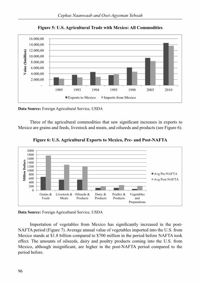
Similar to exports, the imports of these agricultural commodities have significantly increased during the implementation phase of the Agreement. Figure 4 presents the comparison of average values of imports of selected commodities pre- and post-NAFTA. Annual average imports of vegetables, grains and oilseeds have increased by 473%, 215% and 268% respectively since 1994. By the same token, importation of dairy products, and livestock/meats from Canada increased by 760% and 131%,respectively, since NAFTA was signed. Figure 5 shows that U.S. agricultural trade with Mexico has enjoyed an increasing trend since the signing of the Agreement, buoyed by rapid increases in exports of grains and oilseeds. As a result of increased demand for meat in Mexico, poultry and hog producers rely heavily on importation of feed grains from the U.S. as feedstuffs. U.S. exports of feed grains and oilseeds to Mexico increased by 134% during NAFTA compared to the periods immediately before the Agreement came into force. Corn, wheat and rice exports to Mexico have quadrupled in the NAFTA era, which largely reflects the enhanced liberalization of agricultural trade provided by the NAFTA framework. With the exception of 1995, the U.S. maintains a trade surplus in agricultural commodities with Mexico both before and after NAFTA was implemented (Figure 5). Both partners appear to have gained from NAFTA; as U.S. increased its exports to Mexico, imports from Mexico increased by about the same margins.

Figure 4: U.S. Agricultural Imports from Canada, Pre- and Post-NAFTA

0500

100015002000250030003500

Mill

ion

Dol

lars

Avg Pre-NAFTA

Avg Post-NAFTA



96


Figure 5: U.S. Agricultural Trade with Mexico: All Commodities

-2.000,00 4.000,00 6.000,00 8.000,00

10.000,00 12.000,00 14.000,00 16.000,00

1989 1993 1994 1995 1998 2005 2010

Val

ue ($

mill

ion)

Exports to Mexico Imports from Mexico


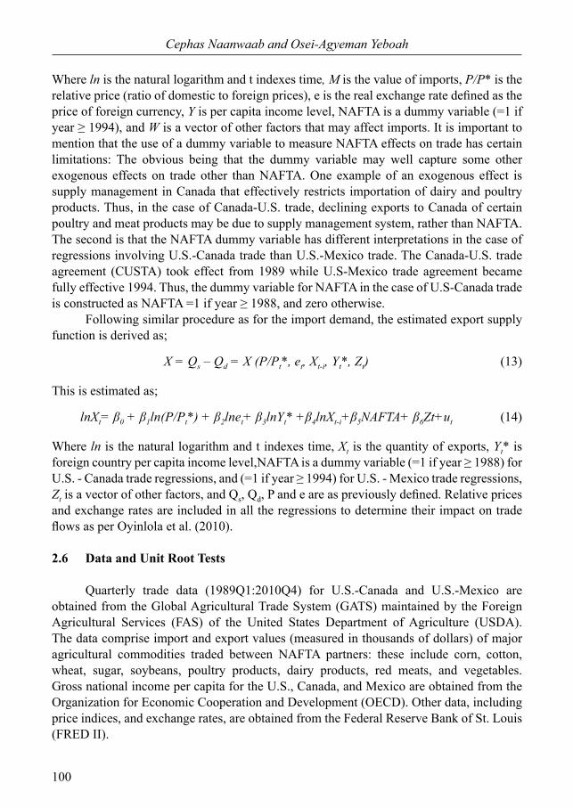
Three of the agricultural commodities that saw significant increases in exports to Mexico are grains and feeds, livestock and meats, and oilseeds and products (see Figure 6).

Figure 6: U.S. Agricultural Exports to Mexico, Pre- and Post-NAFTA

0200400600800

100012001400160018002000

Grains & Feeds

Livestock & Meats

Oilseeds & Products

Dairy & Products

Poultry & Products

Vegetables and

Preparations

Mill

ion

Dol

lars

Avg Pre-NAFTA

Avg Post-NAFTA


Importation of vegetables from Mexico has significantly increased in the post-NAFTA period (Figure 7). Average annual value of vegetables imported into the U.S. from Mexico stands at $1.8 billion compared to $700 million in the period before NAFTA took effect. The amounts of oilseeds, dairy and poultry products coming into the U.S. from Mexico, although insignificant, are higher in the post-NAFTA period compared to the period before.


97


Figure 7: U.S. Agricultural Imports from Mexico, Pre- and Post-NAFTA

0200400600800

100012001400160018002000

Vegetables and

Preparations

Livestock & Meats

Grains & Feeds

Dairy & Products

Oilseeds & Products

Poultry & Products

Mill

ion

Dol

lars

Avg Pre-NAFTA

Ave Post-NAFTA


2.2 Partial Equilibrium Analysis of U.S. Trade with NAFTA partners

To study the effect of NAFTA on US trade with other NAFTA partners, a partial equilibrium model is posited. Partial equilibrium, as opposed to general equilibrium, allows the study of the impact of a trade policy on one sector of the economy. Koo and Kennedy (2005) used partial equilibrium analysis to derive the import demand and export supply functions for a particular commodity or sector of the economy. The information derived from partial equilibrium analysis can be used by policy makers to estimate welfare effects (consumer and producer surpluses) associated with certain trade policies.

2.3 Import Demand Function

The import demand function can be derived as the excess domestic demand for a good. In this context, import demand for a particular commodity is defined at the points where the domestic quantity demanded of the good is greater than the domestic supply, as in Figure 8 below (Koo and Kennedy, 2005). Algebraically, import demand is defined as;

Qm(P,Y) = Qd(P, Y(P)) – Qs(P) = Qm (P, Y) (1)

where Qm(.) is the quantity of the commodity imported as a function of domestic price P and income Y, Qd(.) is the domestic quantity demanded as a function of price P, and income Y, and Qs(P) is the quantity of the good supplied domestically at each price level. It can be proved that the import demand is inversely related to domestic price level, as derived in Figure 8 below.


98


Figure 8: Derivation of import Demand curve

This inverse relationship between import demand and price can also be derived algebraically as;

* 0m d d sQ Q Q QY

P P Y P P

(2)

where the first term on the right is negative by the law of demand, the second term is negative by assumption that the imported good in question is a normal good, such that ∂Qd/∂Y>0 and ∂Y/∂P< 0 because higher prices reduce the consumers real income. Lastly, ∂Qs/∂P is positive by the law of supply. From Figure 8, when the domestic price is $40 per unit, domestic quantity demanded is equal to domestic supply of 30 units, thus, the domestic market clears and import demand is zero. As the price falls to $20 per unit, domestic producers have less incentive to produce and therefore cut supply to 20 units while domestic demand increases to 40 units. The domestic excess demand of 20 units (40-20) is the import demand at the price of $20. As price further decreases to $10, import demand increases to 30 units (45-15).

2.4 Export Supply Function

The export supply function is derived as the horizontal difference between the domestic quantity supplied and domestic quantity demanded of a commodity at any given price. Export supply is positive when the domestic quantity supplied exceeds domestic quantity demanded, and this occurs at price levels at which the domestic price is higher than the international price, thus creating a surplus (excess supply) on the domestic market. The export supply (or excess supply) is zero at the point where the domestic and international prices of the commodity are equalized. Export supply may be derived as;

x s dQ (P) Q (P) – Q (P) (3)


99


where Qx(P) is the quantity of exports of the commodity as a function of price, Qs and Qd are domestic quantity supplied and domestic quantity demanded, respectively.

2.5 Empirical Models

Following Khan and Ross (1977) and Boylan et al. (1980), the import demand is specified as

Mt* = f (Yt, Pmt/Pdt); (4)

Which can be linearized as;

Mt*= α0 + α1Yt + α2Pt +et (5)

Where Mt* is the desired quantity of imports, Ytis the gross domestic product (or income), Pt

is the relative price defined as the ratio of import price (Pmt) to domestic price (Pdt). A partial adjustment mechanism may be introduced into the model in equation 5 above (Doroodian, 1994). This is expressed as;

*

1 1( )t t t t tM M M M M (6)

Where Mt and Mt-1 are actual quantities imported at time t and t-1 respectively, and is the coefficient of adjustment, such that; 0 1 . Substituting equation 5 into equation 6, and rearranging the terms yields the following dynamic import demand equation;

0 1 2 1 (1 )t t t t tM Y P M e (7)

Partial equilibrium analysis is used to model U.S. import demand for agricultural commodities. The following equations represent the domestic market clearing conditions for each commodity;

Qd = Qd (P, Y, e) (8)

Qs = Qs (P, e,W) (9)

Qd = Qs (10)

Assuming that there is a negative price differential between the domestic and international markets, the estimated excess demand or import demand is given as;

Mt = Qd-Qs = M (P/Pt*, et, Yt, Mt-i,Wt) (11)

This is estimated econometrically as;

lnMt= α0 + α1ln(P/Pt*) + α2lnet+ α3 lnYt +α4lnMt-i+α5NAFTA+ α6Wt +εt (12)


100


Where ln is the natural logarithm and t indexes time, M is the value of imports, P/P* is the relative price (ratio of domestic to foreign prices), e is the real exchange rate defined as the price of foreign currency, Y is per capita income level, NAFTA is a dummy variable (=1 if year ≥ 1994), and W is a vector of other factors that may affect imports. It is important to mention that the use of a dummy variable to measure NAFTA effects on trade has certain limitations: The obvious being that the dummy variable may well capture some other exogenous effects on trade other than NAFTA. One example of an exogenous effect is supply management in Canada that effectively restricts importation of dairy and poultry products. Thus, in the case of Canada-U.S. trade, declining exports to Canada of certain poultry and meat products may be due to supply management system, rather than NAFTA. The second is that the NAFTA dummy variable has different interpretations in the case of regressions involving U.S.-Canada trade than U.S.-Mexico trade. The Canada-U.S. trade agreement (CUSTA) took effect from 1989 while U.S-Mexico trade agreement became fully effective 1994. Thus, the dummy variable for NAFTA in the case of U.S-Canada trade is constructed as NAFTA =1 if year ≥ 1988, and zero otherwise. Following similar procedure as for the import demand, the estimated export supply function is derived as;

X = Qs – Qd = X (P/Pt*, et, Xt-i, Yt*, Zt) (13)

This is estimated as;

lnXt= β0 + β1ln(P/Pt*) + β2lnet+ β3lnYt* +β4lnXt-i+β5NAFTA+ β6Zt+ut (14)

Where ln is the natural logarithm and t indexes time, Xt is the quantity of exports, Yt* is foreign country per capita income level,NAFTA is a dummy variable (=1 if year ≥ 1988) for U.S. - Canada trade regressions, and (=1 if year ≥ 1994) for U.S. - Mexico trade regressions, Zt is a vector of other factors, and Qs, Qd, P and e are as previously defined. Relative prices and exchange rates are included in all the regressions to determine their impact on trade flows as per Oyinlola et al. (2010).

2.6 Data and Unit Root Tests

Quarterly trade data (1989Q1:2010Q4) for U.S.-Canada and U.S.-Mexico are obtained from the Global Agricultural Trade System (GATS) maintained by the Foreign Agricultural Services (FAS) of the United States Department of Agriculture (USDA). The data comprise import and export values (measured in thousands of dollars) of major agricultural commodities traded between NAFTA partners: these include corn, cotton, wheat, sugar, soybeans, poultry products, dairy products, red meats, and vegetables. Gross national income per capita for the U.S., Canada, and Mexico are obtained from the Organization for Economic Cooperation and Development (OECD). Other data, including price indices, and exchange rates, are obtained from the Federal Reserve Bank of St. Louis (FRED II).


101


Time series data used in regression analysis should be stationary (Enders, 2004). A stationary time series is one that has a constant mean and variance over time (covariance stationary process). A violation of the stationarity assumption results in a spurious regression, in which the R2 is high and t ratios appear to be significant but the output results have no economic meaning (Granger and Newbold, 1974). The Augmented Dickey-Fuller test, equation (15) below, proposed by Dickey and Fuller (Dickey and Fuller, 1979;Dickey and Fuller, 1981), was performed to check presence of unit roots. The null hypothesis for the ADF unit root test consists of testing 0 . Failure to reject this null hypothesis signifies the presence of a unit root. By this definition, the tests show that all variables are unit root processes, or integrated of order one, I(1). First differencing the variables, thus, achieves required stationary series, or I(0) processes.

0 1 1

pt t j t j tj

y a y y (15)

3. Results and Discussion

3.1 Regression Analysis

The analysis covers top agricultural commoditi es traded in the NAFTA area including corn, wheat, cotton, soy bean, poultry products, dairy products, red meats, sugar, and vegetables. Tables 1 and 2 compare the pre-NAFTA and post-NAFTA average values of trade between the U.S. and Canada for the commodities covered in the regression analysis. The post-NAFTA average values traded are significantly higher than pre-NAFTA values. Similar analysis (not shown for brevity) of pre- and post-NAFTA trade between the U.S. and Mexico reveal the same findings as for U.S. –Canada trade.

Table 1: Pre- and Post-NAFTA Analysis of U.S. Exports to Canada

Exports Avg. Pre-NAFTA Avg. Post-NAFTA Difference (Value $mil) (Value $mil) (Value $mil)

Corn 15635.75 57461.74 41825.99* Cotton 14888.15 16616.7 1728.55* Wheat 507.1 1110.5 603.4* Soya bean 10574 23004.39 12430.39* Vegetables (fresh) 142125.3 271677.8 129552.5* Dairy Products 11392.9 65656.48 54263.58*Poultry Products 46813.5 97236.56 50423.06*

Red Meats 92702.75 194819.8 102117.05*

*=Difference statistically significant at the 5% level


102


Table 2: Pre- and Post-NAFTA Analysis of U.S. Imports from Canada

Imports Avg. Pre-NAFTA Avg. Post-NAFTA Difference (Value $mil) (Value $mil) (Value $mil)

Corn 4297.6 8802.03 4504.43*Wheat 30067.7 88222.53 58154.83*Soya bean 4983 12430.59 7447.59*Vegetables (fresh) 24313 144306.5 119993.5*Dairy Products 7963.45 68261.18 60297.73*Poultry Products 9167.9 36694.14 27526.24*

Red Meats 160764.9 416805.8 256040.9*

*=Difference statistically significant at the 5% level

Regression analyses show mixed findings regarding the direction of NAFTA effects on agricultural commodity trade between NAFTA partners. A number of econometric specifications were tried to determine if the mixed sign effects of NAFTA could be due to a misspecification, but all turned up almost similar results. Autocorrelation and heteroskedasticity were identified as potential issues that could be causing this mixed signs. Estimating the models in first differences did not change the signs. Consequently, we employed Prais-Winsten and Cochrane-Orcutt transformations to deal with the time series issues relating to autocorrelation. In Tables 3A and 3B, the results of regression analyses of U.S. agricultural commodity trade with Canada are presented, while Tables 4A and 4B present similar regression analyses for U.S. – Mexico trade. Tables 3A and 4A show estimates of the export supply functions for U.S. exports to Canada and Mexico, respectively. The regression results show that since NAFTA’s inception, U.S. corn and poultry product exports to Canada have significantly declined, while U.S. exports of corn to Mexico has significantly increased. Before NAFTA, Mexico strictly regulated the importation of corn from U.S. and Canada using import licensing requirements. Under NAFTA, tariffs were replaced with duty-free tariff rate quotas during the period of 1994-1997 and eventually eliminated by 2008. The increased trade in corn is a reflection of the removal of these trade barriers. The impact of NAFTA on U.S. exports of cotton to Canada is positive but not significant. NAFTA’s effect on the exports of U.S. soy bean to Canada is negative but statistically insignificant. The regression results also show that the effect of NAFTA on U.S. exports of wheat, soy bean, and poultry products to Mexico is not statistically significant. U.S. dollar depreciation against the Canadian dollar increases U.S. exports of cotton to Canada, and in the same vein U.S. dollar depreciation against the Mexican Peso increases U.S. exports of poultry products to Mexico. The exchange rate effect is however negative in the export of poultry products to Canada, but insignificant with regard to U.S. exports of corn, soy bean and wheat to Mexico. Increases in gross national income per


103


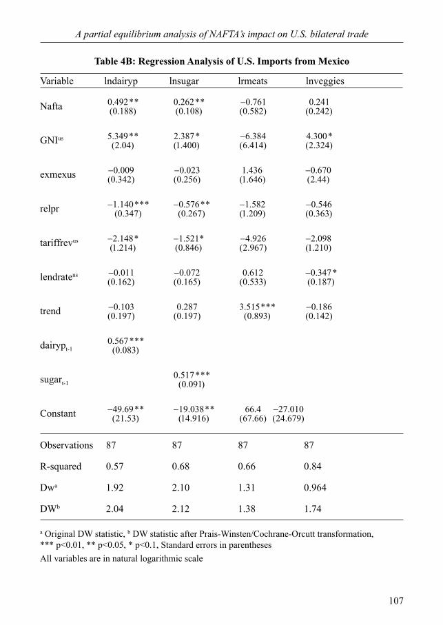
capita in Canada lead to increases in U.S. exports, while U.S. exports of corn to Mexico increases with increasing per capita incomes in Mexico. Similar findings of the effect of GDP on trade flows have been reported for trade between the E.U. and the Western Balkans (Botrić, 2013). Matchaya et al. (2013) found evidence that GDP (income) growth leads to increased trade in the case of imports to Malawi. Other explanatory variables, namely, relative prices, average tariffs, and lending rates are shown to have mixed effects on U.S. exports to Canada and Mexico. Similarly, Tables 3B and 4B show the estimated import demand functions for U.S. imports from Canada and Mexico, respectively. In Table 3B we present the estimated import demand functions for U.S. imports of dairy products, poultry products, red meats, and wheat from Canada. The effect of NAFTA on the exports of all these products is negative but statistically significant only for wheat imports from Canada and insignificant for dairy, poultry and read meats. Further results from Table 3B show the income effect is positive and significant for U.S. imports of poultry and red meats from Canada, while the exchange rate is insignificant, except for red meats, in which case it has a positive effect, opposite of what we would expect for imports. The relative price effect is negative and significant for dairy products and wheat imports from Canada, indicating that lower domestic prices of these commodities result in an increased excess demand, and consequently increased importation. In Table 4B we present regression results of U.S. imports of dairy products, sugar and related products, red meats, and vegetables from Mexico. The results show that U.S. imports of dairy products and sugar have significantly increased under NAFTA than in the period preceding the agreement. There is no significant impact of NAFTA on the importation of red meats and vegetables in general from Mexico. The income and relative price effects are significant in the dairy and sugar equations with the expected signs: Increase in U.S. per capita income increases the amounts of each commodity imported, which conform to the assumption that these are normal goods. Also, lower domestic prices lead to increased domestic demand, and hence higher import demand. The exchange rate effect is negative as expected but statistically insignificant. All things remaining constant, it is expected that an appreciation of the dollar increases the purchasing power of U.S. consumers; as such we would expect an increase in imports. In other words, a depreciation of the peso increases Mexican exports (i.e. increases in U.S. imports). The average tariff rate does have a marginal effect on U.S. imports but the lending rate does not significantly affect the imports of dairy products, sugar products, red meats, and vegetables from Mexico. The regression results also show mixed effects with regard to the tariff revenues (a proxy for tariff rates) in most of the models estimated. The effect of Canada’s tariffs is positive and significant in the case of U.S. exports of corn to Canada (Table 3A). On the other hand U.S. tariff has a negative effect on imports of poultry and red meats from Canada and positively related to imports of wheat (Table 3B). Mexico’s tariff rate negatively impacted U.S. exports of corn, soy bean and wheat to Mexico (Table 4A). In the same vein, Table 4B shows that U.S. tariff rate negatively affected imports of dairy, sugar, and red meats from Mexico.


104


Table 3A: Regression Analysis of U.S. Exports to Canada

Variable lncorn lncotton lnsoyb lnpoultry

Nafta .844**(0.384) 0.425

(0.369) 0.818(0.608) 0.202**

(0.098)

excaus 0.963(0.592) 1.947***

(0.667) 1.44(0.916) 0.389**

(0.157)

GNIcan 5.673***(1.842) 2.75*

(1.635) 6.61**(2.52) 0.156

(0.409)

lendratecan 0.537*(0.285) 0.815***

(0.277) 0.634(0.401) 0.012

(0.067)

tariffrevcan 2.067***(0.551) 0.293

(0.489) 0.311(0.742) 0.169

(0.133)

relpr 20.88***(7.02)

20.42***(7.26) 4.847

(9.878) 3.407*

(1.739)

trend 0.054(0.323) 0.623*

(0.321) 0.44(0.376) 0.309***

(0.059)

cornt-1 0.486***(0.110)

cornt-2 0.327***(0.106)

cottont-1 0.552***(0.110)

cottont-2 0.018(0.104)

soybt-1 0.416***(0.111)

Constant 49.47***(17.93)

28.72*(16.44)

58.02**24.91

1 2.40***(4.204)

Observations 85 85 85 87

R-squared 0.75 0.75 0.63 0.89

DWa 1.94 1.95 2.04 1.83

DWb 1.97 1.95 1.98 1.95

a Original DW statistic, b DW statistic after Prais-Winsten/Cochrane-Orcutt transformation, *** p<0.01, ** p<0.05, * p<0.1, Standard errors in parenthesesAll variables are in natural logarithmic scale


105


Table 3B: Regression Analysis of U.S. Imports from Canada

Variable lndairyp lnpoultry lnrmeats lnwheat

Nafta 0.168(0.163) 0.056

(0.075) 0.055

(0.066) 0.604***

(0.217)

excaus 0.002(0.543) 0.226

(0.146) 0.485***

(0.145) 0.227(0.346)

GNIus 1.98(1.846) 1.358*

(0.749) 1.536**(0.732) 3.11*

(1.81)

lendrateus 0.197(0.141) 0.063

(0.057) 0.038

(0.045) 0.057(0.144)

tariffrevus 0.718(0692) 0.718*

(0.349) 0.262

(0.290) 2.458**

(0.994)

relpr 8.584**(3.637) 0.173

(1.374) 1.129

(1.333) 27.12***(5.616)

trend 0.186(0.155) 0.061

(0.053) 0.055(0.049) 0.311*

(0.156)

poultryt-1 0.654***(0.092)

rmeatst-1 0.555***(0.105)

wheatt-1 0.403***(0.095)

Constant 9.311(9.725) 10.43

(7.142) 35.76*

(20.02)


R-squared 0.08 0.98 0.98 0.83

DWa 1.16 2.16 2.15 2.11

DWb 2.28 2.09 2.01 2.01



106


Table 4A: Regression Analysis of U.S. Exports to Mexico

Variable lncorn lnsoyb lnwheat lnpoultry

Nafta 1.244***(0.239) 0.288

(0.351) 0.501(0.552) 0.007

(0.184)

exmeus 0.340(0.426) 0.798

(0.719) 1.856

(1.122) 1.059***

(0.286)

GNImex 3.111**(1.346) 1.515

(2.349) 0.394(3.704) 1.558

(1.272)

relpr 1.096***(4.08) 0.996**

(0.499) 0.497(0.799) 0.602

(0.642)

tariffrevmex 0.699***(0.211)

0.590**(0.28)

0.542(0.445) 0.364*

(0.213)

lendratemex 0.133(0.116) 9.3 06

(0.201)E 0.205

(0.315) 0.122

(0.086)

trend 1.317***(0.312)

0.344(0.313) 1.035**

(0.512) 0.455**(0.204)

cornt-1 0.783***(0.105)

cornt-2 0.251**(0.099)

Constant 16.51(11.71) 3.683

(20.31) 10.51(31.97)


R-squared 0.91 0.56 0.65 0.18

Dwa 2.13 2.19 2.22 1.06

Dwb 1.93 2.06 2.58 2.3



107


Table 4B: Regression Analysis of U.S. Imports from Mexico

Variable lndairyp lnsugar lrmeats lnveggies

Nafta 0.492**(0.188) 0.262**

(0.108) 0.761(0.582)

0.241

(0.242)

GNIus 5.349**(2.04) 2.387*

(1.400) 6.384

(6.414)

4.300*

(2.324)

exmexus 0.009(0.342) 0.023

(0.256) 1.436

(1.646) 0.670

(2.44)

relpr 1.140***(0.347)

0.576**(0.267) 1.582

(1.209) 0.546

(0.363)

tariffrevus 2.148*(1.214) 1.521*

(0.846) 4.926

(2.967)

2.098

(1.210)

lendrateus 0.011(0.162) 0.072

(0.165) 0.612

(0.533) 0.347*(0.187)

trend 0.103(0.197) 0.287

(0.197) 3.515***(0.893) 0.186

(0.142)

dairypt-1 0.567***

(0.083)

sugart-1 0.517***(0.091)

Constant 49.69**(21.53) 19.038**

(14.916) 66.4

(67.66) 27.010(24.679)


R-squared 0.57 0.68 0.66 0.84

Dwa 1.92 2.10 1.31 0.964

DWb 2.04 2.12 1.38 1.74



108


Table 5: Description of Variables Used in the Models

Variable Description Data SourceExcaus U.S.-Canada real exchange rate ($US/$can) Federal Reserve BankExmeus U.S.-Mexico real exchange rate ($US/peso) Federal Reserve BankGNI Gross national income per capita OECDLendrate Domestic lending rate (cost of borrowing) OECDTariffrev Average tariff revenues collected OECDRelpr Relative price (domestic/foreign price ratio) Federal Reserve BankTrend Time trend N/ADairyp Quantity of Dairy products GATS-FASRmeats Quantity of Red meats products GATS-FASVeggies Quantity of Vegetables GATS-FASCorn Quantity of corn GATS-FASSugar Quantity of sugar GATS-FASSoyb Quantity of soy beans GATS-FAS

3.2 Counterfactual Analysis

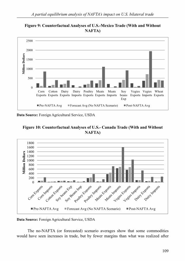
The mixed findings from the regression analyses contrast with the all-positive effects of NAFTA shown in Tables 1 and 2, as well as in the preceding graphical analyses. A plausible explanation for this could be the failure of the dummy variable (NAFTA=1 for years>1994) to pick up the true effect of NAFTA on traded commodities in a regression analytic framework. An alternative to the regression analyses, then, is to perform counterfactual analyses, whereby, we compare the realized trade values (for each commodity) to what would have obtained, had NAFTA not come into existence. Essentially, with counterfactual analyses, we aim to answer the question: What would have been the path of U.S. agricultural trade with Canada and Mexico had NAFTA not existed? To do this, we would have to assume that NAFTA did not exist at all, and then, using the historical trade data up until 1993, forecast the trend that trade in each commodity would have taken without the NAFTA agreement. This is implemented by conducting a three-period moving average forecast of trade for ten years beyond 1993. Comparing these forecasted no-NAFTA trade data to the actual (or realized) data post-NAFTA reveals that NAFTA indeed had a positive effect on the trade of most of these commodities. Figures 9 and 10 present a graphical summary of the counterfactual analyses for different commodities. These graphs compare the pre-NAFTA, forecast (No NAFTA), and the post-NAFTA averages for each commodity. What is clear from these graphs is that for almost all the commodities, post-NAFTA averages are higher than both the pre-NAFTA and forecasted values.


109


Figure 9: Counterfactual Analyses of U.S.-Mexico Trade (With and Without NAFTA)

0

500

1000

1500

2000

2500

Corn Exports

Cotton Exports

Dairy Exports

Dairy Imports

Poultry Exports

Meats Exports

Meats Imports

Soy beans Exp

Vegies Exports

Vegies Imports

Wheat Exports

Mill

ion

Dol

lars

Pre-NAFTA Avg Forecast Avg (No NAFTA Scenario) Post-NAFTA Avg


Figure 10: Counterfactual Analyses of U.S.- Canada Trade (With and Without NAFTA)

0200400600800

10001200140016001800

Mill

ion

Dol

lars

Pre-NAFTA Avg Forecast Avg (No NAFTA Scenario) Post-NAFTA Avg


The no-NAFTA (or forecasted) scenario averages show that some commodities would have seen increases in trade, but by fewer margins than what was realized after


110


NAFTA’s implementation. For example, U.S. trade in poultry products, meats and vegetables with Canada is forecasted to be higher than the case before NAFTA came into existence. Similarly, U.S. trade in cotton, wheat, meats, soybeans, and vegetables with Mexico are higher in the forecasted scenario than pre-NAFTA case, indicating that trade in these commodities would have continued an upward trend whether or not NAFTA existed. Overall, however, post-NAFTA averages are significantly higher than pre-NAFTA or forecasted averages, an indication of the positive effect that NAFTA had on trade between the U.S. and NAFTA partners.

4. Conclusion

This paper presents an empirical analysis of the effects of the North American Free trade Agreement (NAFTA) on agricultural commodity trade between U.S.-Canada on the one hand, and U.S.-Mexico on the other hand. Using quarterly data from 1989 to 2010, we explore, using different approaches, the trends in agricultural commodity trade between NAFTA partners. Overall agricultural trade has been increasing since the inception of the agreement, as tariff and non-tariff barriers were gradually reduced. By 2008, all tariff and non-tariff barriers on agricultural commodities were eliminated, thus, allowing unfettered trade among the signatories of the agreement. Graphical analyses of the trends in trade indicate that most of the agricultural commodities have seen increased trade, with post-NAFTA average quantities traded far exceeding pre-NAFTA averages. Regression analysis, however, show mixed effects of NAFTA on trade, which is attributed to the inability of the dummy variable for NAFTA to pick up the true effect of the agreement. The regression results show that since NAFTA’s implementation, U.S. exports of corn and poultry products to Canada significantly decreased, while U.S. exports of corn to Mexico significantly increased. At the same time, while U.S. importation of sugar and dairy products from Mexico significantly increased following NAFTA, imports of wheat and poultry products from Canada significantly decreased. More robust estimation approaches, other than the dummy-variable approach, might accurately capture the positive effects observed in the graphical analyses. For this reason, a counterfactual approach, using pre-NAFTA data to forecast the trends in trade, assuming NAFTA had not existed, is used to augment the regression analysis. We find that increases in trade would have been far less than what we observed in the actual data after NAFTA came into existence.

Acknowledgement

The paper has benefitted immensely from the constructive suggestions of two anonymous reviewers, to whom we gracefully acknowledge.


111


References

Botrić, V., 2013, Determinants of Intra-industry Trade between Western Balkans and EU-15: Evidence from Bilateral Data, International Journal of Economic Sciences and Applied Research, 6, 2, pp. 7-23.

Boylan,T., Cuddy, M. and O’Muircheartaigh, I., 1980, ‘The Functional Form of the Aggregate Import Demand Equation: A Comparison of Three European Economies’, Journal of International Economics, 10, 4, pp. 561-566.

Burfisher, M.E. and Jones, E.A. (eds.), 1998, ‘Regional Trade Agreements and U.S. Agriculture’, Market and Trade Economics Division, Economic Research Service, U.S. Department of Agriculture, Agricultural Information Bulletin No. 745.

Burfisher, M.E., Robinson, S. and Thierfelder. K., 2001, ‘The Impact of NAFTA on the United States’, Journal of Economic Perspectives, 15, 1, pp. 125-144.

Davey, W.J., 2005, ‘Regional Trade Agreements and the WTO: General Observations and NAFTA Lessons for Asia’, Illinois Public Law and Legal Theory Research Paper Series, Research Paper No. 05-18.

Dickey, D.A. and Fuller, W.A., 1979, ‘Distributions of the Estimators for Autoregressive Time Series with a Unit Root’, Journal of the American Statistical Association, 74, pp. 427-431.

Dickey, D.A. and Fuller, W.A., 1981, ‘Likelihood ratio statistics for autoregressive time series with a unit root’, Econometrica, 49, pp. 1057-1072.

Doroodian, K., Koshal, R.K. and Al-Muhanna S., 1994, ‘An Examination of the Traditional Aggregate Import Demand Function for Saudi Arabia’, Applied Economics, 26, 9, pp. 909-915.

Enders, W., 2004, Applied Econometric Time Series, 2nd ed. John Wiley & Sons Inc., pp. 171.

ERS (Economic Research Service of the USDA), 1999. ‘NAFTA: The Record to Date’, World Agriculture and Trade, Agricultural Outlook, September, 1999.

Granger, C. and Newbold, P., 1974, ‘Spurious Regressions in Econometrics’, Journal of Econometrics, 2, pp. 111-120.

Hejazi, W. and Safarian, A.E., 2005, ‘NAFTA Effects and the Level of Development’, Journal of Business Research, 58, 12, pp. 1741-1749.

Hillberry, R.H. and McDaniel, C.A., 2002, ‘A Decomposition of North American Trade Growth since NAFTA’, International Trade Commission.Office of Economics Working Paper, No. 2002-12-A.

Hinojosa-Ojeda, R., Runsten, D., De Paolis, F. and Kamel, N., 2000, ‘The U.S. Employment Impacts of North American Integration after NAFTA: A Partial Equilibrium Approach’, Unpublished manuscript, North American Integration and Development Center, School of Public Policy and Social Research, UCLA.

Hummels, D. and Klenow, P.J., 2002, ‘The Variety and Quality of a Nation’s Trade’, National Bureau of Economic Research (NBER) Working Paper 8712.


112


Khan, M.S. & Ross, K., 1977, ‘The Functional form of the Aggregate Import Demand Equation’, Journal of International Economics, 7, 2, pp. 149-160.

Koo, W.W. and Kennedy, P.L., 2005, International Trade and Agriculture, Blackwell Publishing.

Matchaya, G. C., Chilonda, P. and Nhelengethwa, S., 2013, ‘International Trade and Income in Malawi: A Co-integration and Causality Approach’, International Journal of Economic Sciences and Applied Research, 6, 2, pp. 125-147.

McDaniel, C.A. and Agama, L-A., 2003, ‘The NAFTA Preference and U.S. - Mexico Trade: Aggregate-Level Analysis’, The World Economy, 26, 7, pp. 939-955.

OECD (Organization for Economic Co-operation and Development), 2001, ‘Regional Integration: Observed Trade and other Economic Effects’, OECD Doc, TD/TC/WP (2001)19/Final.

Oyinlola, M. A., Adeniyi, O. and Omisakin, O., 2010, Responsiveness of Trade Flows to Changes in Exchange rate and Relative prices: Evidence from Nigeria, International Journal of Economic Sciences and Applied Research, 3, 2, pp. 123-141.

USDA (U.S. Department of Agriculture), 1997, NAFTA. WRS-97-2, Washington, DC.USDA-FAS (Foreign Agricultural Service of the U.S. Department of Agriculture), 2012,

Global Agricultural Trade System (GATS Database), http://www.fas.usda.gov/gats/default.aspx.

Viner, J., 1950,The Customs Union Issue, New York, Carnegie Endowment for International Peace.

Zahniser, S. and Link, J. (eds.), 2002, ‘Effects of North American Free Trade Agreement on Agriculture and the Rural Economy’, A Report from the Economic Research Service, ERS/USDA, WRS (02-01).

Zahniser, S. and Roe A. (eds.), 2011, ‘NAFTA at 17: Full Implementation leads to Increased Trade and Integration’, A Report from the Economic Research Service, ERS/USDA, WRS (11-01).


a partial equilibrium analysis of nafta’s impact on u.s...

Documents