a penalty method for a linear koiter shell model

HAL Id: hal-01956616https://hal.archives-ouvertes.fr/hal-01956616

Submitted on 16 Dec 2018

HAL is a multi-disciplinary open accessarchive for the deposit and dissemination of sci-entific research documents, whether they are pub-lished or not. The documents may come fromteaching and research institutions in France orabroad, or from public or private research centers.

L’archive ouverte pluridisciplinaire HAL, estdestinée au dépôt et à la diffusion de documentsscientifiques de niveau recherche, publiés ou non,émanant des établissements d’enseignement et derecherche français ou étrangers, des laboratoirespublics ou privés.

A penalty method for a linear Koiter shell modelIsmail Merabet, Serge Nicaise

To cite this version:Ismail Merabet, Serge Nicaise. A penalty method for a linear Koiter shell model. ESAIM:Mathematical Modelling and Numerical Analysis, EDP Sciences, 2017, 51 (5), pp.1783-1803.�10.1051/m2an/2017009�. �hal-01956616�

https://hal.archives-ouvertes.fr/hal-01956616

https://hal.archives-ouvertes.fr

ESAIM: M2AN 51 (2017) 1783–1803 ESAIM: Mathematical Modelling and Numerical AnalysisDOI: 10.1051/m2an/2017009 www.esaim-m2an.org

A PENALTY METHOD FOR A LINEAR KOITER SHELL MODEL

Ismail Merabet1and Serge Nicaise

2

Abstract. In this paper a penalized method and its approximation by finite element method areproposed to solve Koiter’s equations for a thin linearly elastic shell. In addition to existence anduniqueness results of solutions of the continuous and the discrete problems we derive some a priori errorestimates. We are especially interested in the behavior of the solution when the penalty parameter goesto zero. We propose here a new formulation that leads to a quasi optimal and uniform error estimatewith respect to the penalized parameter. In other words, we are able to show that this method convergesuniformly with respect to the penalized parameter and to the mesh size. Numerical tests that validateand illustrate our approach are given.

Mathematics Subject Classification. 74K25, 65N30, 74S05.

Received April 22, 2016. Accepted March 7, 2017.

1. Introduction

Linear models of thin elastic shells can be classified into two different families: the Kirchhoff−Love theoryand the Reissner−Mindlin theory. The Reissner−Mindlin plates theory was generalized to shells by P. M.Naghdi [24]. In the framework of the Kirchhoff−Love theory, Koiter [19] derived a two dimensional model forlinearly elastic shells. The comparison between Koiter’s and Naghdi’s model leads to the comparison between theKirchhoff−Love and Reissner−Mindlin theories. For “moderately” thin shells, the Naghdi model is better thanthe Koiter model, because it takes in account the transverse shear. Naghdi’s model is also preferred becauseit better represents boundary conditions (it can distinguish between hard and soft simple support). But forvery thin shells and for very smooth solutions, Koiter’s model is better than Naghdi’s model. Koiter’s model isactually one of the most currently used for numerical computations, it contains both membrane and bendingeffects coupled at different order of magnitudes. W.T Koiter based his derivation on two a priori assumptions,one of a mechanical nature about the stresses inside the shell during the deformation. It states that if thethickness is small enough, then the state of stress is approximately planar and parallel to the tangent plane tothe middle surface S. The second a priori assumption is of geometrical nature and states that the normal vectorto the undeformed middle surface, considered as a set of particles of the shell, remains on a line normal to thedeformed middle surface and the lengths are unmodified along this line after the deformation has taken place.For very thin elastic shells, Koiter’s model was rigorously justified (see [15, 16]). For the classical formulation,

Keywords and phrases. Shell theory, Koiter’s model, finite elements error analysis.

1 LMA, Universite Kasi Merbah – Ouargla, 30000, Algerie. [email protected] LAMAV, Universite de Valenciennes et du Hainaut-Cambresis, Valenciennes cedex 9, [email protected]

Article published by EDP Sciences c© EDP Sciences, SMAI 2017

https://doi.org/10.1051/m2an/2017009

http://www.esaim-m2an.org

http://www.edpsciences.org

1784 I. MERABET AND S. NICAISE

the problem was formulated by the use of the covariant and contravariant components representation of theunknowns and a huge literature is dedicated to its approximation by various finite element methods. Thisformulation requires that the shell has a C3-middle surface at least, which is restrictive from the point ofview of the applications (see [7]). The use of C1 elements gives good results, but the main drawbacks are thecomplexity of the elements and the poor stability for irregular solution. A second type of approximation, so-called non conforming approximation, is based on the idea of relaxing the continuity of functions and of theirnormal derivatives along the boundaries of elements. The most well-known elements in this class is the discreteKirchhoff triangle DKT (discrete Kirchhoff triangle) which was used in [4] to approximate a Koiter model.Numerical locking is a serious drawback for this element when considering bending-dominated shells with verysmall thickness.

A new formulation was introduced in [7]; it is based on the idea of using a local basis-free formulation inwhich the unknowns are described in Cartesian coordinates. This new formulation allows to handle shells witha W 2,∞-middle surface. Its approximation by finite element methods was considered in [6] and implementedusing the finite element software Freefem++ [17]. This new formulation enters in the family of problems wherethe constraint is distributed over the domain, like the divergence-free constraint for incompressible Stokes flows.

Penalty methods are already efficiently used to handle constrained problems (see [20]). Roughly speaking, apenalty method consists in adding an extra term, the penalty term p−1b(u, v)3, to the variational formulationin order to handle the constraint. In [3] a penalty approach was used to prescribe non-homogeneous Dirichletboundary conditions on the boundary. Recently, in the finite element context, some interesting contributionsof the penalty method were presented in [23] where the author is also interested to geometrical constraints,namely interested in solving an elliptic problem on a simply shaped domain with holes. He highlights thedifference between two kinds of penalty problems; closed and non closed penalty problems, i.e., the case whenb(u, v) = (Bu,Bv) with B a linear operator with closed range or not. At the continuous level, the closed penaltyproblem was proved to be more accurate. In the same spirit, we reformulate Koiter’s equation in Cartesiancoordinates with a “closed penalization”. Note that a non-closed penalization was already considered in [6].We intend to show that the corresponding finite element method converges in the energy norm uniformly withrespect to the mesh size and to the penalized parameter.

This paper is organized as follow: in Section 2, we first briefly recall the geometry of the surface as wellas Koiter’s shell model formulated in Cartesian coordinates and we point out the main difficulty for whichthe original problem can not be implemented in a conforming way. In Section 3 we introduce a penalizedformulation of Koiter’s model in which a new functional space and a new bilinear form are introduced. Weprove that the penalized problem is well-posed. We present in Section 4 its finite element discretization andprove its well-posedness and its consistency. Hence the convergence of the method depend on its stability,which involves boundedness and coercivity of the bilinear form. As a result, for this problem, error estimatescannot be uniform in p. In Section 5 we introduce a new formulation for which we are able to show that themethod converges uniformly with respect to the penalized parameter and the mesh size. Finally, we presentsome numerical tests in Section 6 that validate and illustrate our approach.

In the whole paper, the notation a � b is used for the estimate a ≤ c b, where c is a generic constant thatdoes not depend on any mesh-size or penalized parameter. The convention of summation of repeated indices,which run from 1 to 2 when they are Greek is used.

2. The linear Koiter model for elastic shells

2.1. The continuous problem

Let (e1, e2, e3) be the canonical orthogonal basis of R3, u · v the inner product of R3, u× v the vector productof u and v. For a given domain ω of R2 with a C1,1 boundary, we consider a shell whose middle surface S is

3The parameter p is 0 < p < 1 and is supposed to tend to zero.

A PENALTY METHOD FOR A LINEAR KOITER SHELL MODEL 1785

given byS = ϕ (ω) where ϕ ∈W 2,∞ (ω,R3

)(2.1)

where Wm,p denotes the usual Sobolev space. ϕ is supposed to be a one-to-one mapping such that the twovectors4

aα = ∂αϕ, α = 1, 2 (2.2)

are linearly independent. The normal vector a3 is given by

a3 =a1 × a2

|a1 × a2|· (2.3)

The contravariant basis ai is defined by the relation

ai · aj = δji , δj

i being the Kronecker symbol. (2.4)

The covariant and contravariant components of the metric (or the fist fundamental form) are given by:

(aαβ) = (aα · aβ) and (aαβ) = (aαβ)−1, a = det(aαβ). (2.5)√a is the area element of the midsurface in the chart. The length element � on the boundary ∂ω is given by√aαβτατβ , (τ1, τ2) being the covariant coordinates of a unit vector tangent to ∂ω.The second fundamental form of the surface is given in covariant components by

bαβ = a3 · ∂βaα = −aα · ∂βa3. (2.6)

The Christoffel symbols of the surface Γ γαβ take the form

Γ γαβ = Γ γ

βα = aγ · ∂βaα = aγ · ∂αaβ. (2.7)

We consider here the case of a homogeneous, isotropic material with Young modulus E > 0 and Poissonratio ν, 0 ≤ ν < 1

2 . We also denote by ε the thickness of the shell which is assumed to be constant and positive.Let aαβρσ denote the contravariant components of the elasticity tensor, its components are given by

aαβρσ =E

2(1 + ν)(aαρaβσ + aασaβρ) +

Eν

2(1 − ν2)aαβaρσ . (2.8)

We note that the Assumption (2.1) on the chart is made such that each component of the elasticity tensor belongsto W 1,∞. Moreover, this tensor satisfies the usual symmetry properties and is uniformly strictly positive i.e.,there exists a positive constant c0 such that

aαβρσταβτρσ ≥ c0|τ |2 a.e. in ω, ∀τ, symmetric tensor of order 2. (2.9)

Let u ∈ H1(ω,R3) be the middle surface displacement. Following [7], the covariant components of the changeof metric tensor and the covariant components of the change of curvature tensor are respectively defined by

γαβ (u) =12

(∂αu · aβ + ∂βu · aα) , (2.10)

Υαβ (u) =(∂αβu− Γ ρ

αβ∂ρu)· a3 . (2.11)

We finally introduce respectively the stress resultant and the stress couple

nαβ(u) = εaαβρσγαβ(u), (2.12)

mαβ(u) =ε3

12aαβρσΥαβ(u). (2.13)

4For simplicity, here and below, we omit x in the previous notations aα(x), a3(x), . . .


2.2. The variational formulation for a totally clamped shell

The functional space for Koiter’s solution is H1(ω)×H1(ω)×H2(ω), when the classical formulation is usedand the totally clamping condition reads

ui = ∂νu3 = 0, on ∂ω (2.14)

where ∂ν denotes the normal derivative on the boundary. Blouza and Le Dret in [7], rewrite the condition (2.14)in a simpler and more intrinsic fashion that makes sense in the context of shells with little regularity; the newclamping condition reads5

u = 0 on ∂ω and ∂αu · a3 = 0 in H1/2(∂ω). (2.15)

Therefor, the functional space V(ω), which is appropriate for shell with little regularity, reads

V(ω) ={v ∈ H1

0

(ω,R3

), ∂αv · a3 ∈ H1

0 (ω)}, (2.16)

equipped with the norm:

‖v‖V(ω) =

(‖v‖2

H1(ω,R3) + ‖∂αv · a3‖2H1(ω)

) 12. (2.17)

The variational formulation of the problem corresponding to the linear Koiter model for shells with littleregularity reads: {

Find u ∈ V(ω) such thata (u, v) = L (v) , ∀v ∈ V(ω),

(2.18)

where,

a (u, v) =∫

ω

(nρσ (u)γρσ (v) +mρσ (u)Υρσ (v))√adx, (2.19)

L (v) =∫

ω

f · v√adx. (2.20)

Theorem 2.1 [7]. Let f ∈ L2(ω,R3) be a given force resultant density. Then the variational problem (2.18) hasa unique solution in V(ω).

Recently, a more realistic formulation was proposed by considering the terms ∂αu·a3 as independent unknownssay rα. Then it is clear that, if sα := ∂αv · a3, the vector s := sαa

α belongs to the space H10 (ω,R3) provided

that v belongs to V(ω). A straightforward calculus amounts to rewrite the new change of curvature tensor andthe stress couple as follows:

Υαβ(u) := χαβ (u, r) :=12

(∂αu · ∂βa3 + ∂βu · ∂αa3) +12

(∂αr · aβ + ∂βr · aα) , (2.21)

:= θαβ(u) + γαβ(r) (2.22)

mαβ(u) := mαβ(u, r) :=ε3

12aαβρσχαβ(u, r) (2.23)

and to reformulate the problem (2.18) as follows:

{Find U = (u, r) ∈ W(ω) such that

a ((u, r) ; (v, s)) = L ((v, s)) , ∀V = (v, s) ∈ W(ω),(2.24)

5The condition (2.15) coincides with the classical clamping condition for ϕ smooth.


where,

W(ω) ={(v, s) ∈ (H1

0

(ω,R3

))2 | s+ (∂αv · a3)aα = 0 a.e in ω

}, (2.25)

a ((u, r) ; (v, s)) =∫

ω

(nρσ (u)γρσ (v) +mρσ (U)χρσ (V ))√adx, (2.26)

L ((v, s)) =∫

ω

f · v√adx. (2.27)

Remark 2.2. Note that, if (v, s) ∈ W(ω) the constraint

s+ (∂αv · a3)aα = 0 a.e, in ω, (2.28)

ors · aα + (∂αv · a3) = 0 a.e, in ω, α = 1, 2 (2.29)

cannot be implemented in a standard conforming way (see [6]). This amounts to say that the problem (2.24)cannot be approximated by conforming methods for a general shell.

3. A penalized version

According to Remark 2.2, in order to avoid the constraint (2.28), as alternative approach we propose tointroduce a penalized version of (2.24). This means that we reformulate the original constrained problem as anunconstrained one.

Let us consider the functional space:

X(ω) = {(v, s) ∈ H10

(ω,R3

)×H1

0 (ω,R3), ∂αv · a3 ∈ H10 (ω)} (3.1)

equipped with the norm

‖(v, s)‖X(ω) =

(‖v‖2

H1(ω,R3) + ‖s‖2H1(ω,R3) + ‖∂αv · a3‖2

H1(ω)

) 12. (3.2)

Clearly, equipped with this norm, X(ω) is a Hilbert space.Let p ∈ R, 0 < p ≤ 1. We consider the following variational problem:{

Find Up = (up, rp) ∈ X(ω) such thata(Up, V ) + (1 + p−1)b(Up, V ) = L(V ), ∀V ∈ X(ω).

(3.3)

For W = (w, t), V = (v, s) ∈ X(ω), the bilinear form b(·, ·) reads

b(W,V ) =∫

ω

∇(t+ (∂αw · a3)aα) : ∇(s+ (∂αv · a3)aα)dx (3.4)

Here, for v = (v1, v2, v3) ∈ H1(ω,R3), we have set

∇v =

⎛⎜⎝∂1v1 ∂2v1

∂1v2 ∂2v2

∂1v3 ∂2v3

⎞⎟⎠ and A : B =

∑α,j

AαjBαj = tr(ABT )

Note that the space H10 (ω,R3) has the inner product:

(u, v)H10 (ω,R3) =

∫ω

∇u : ∇v dx =∑

i

∫ω

∇ui · ∇vi dx =∑α,j

∫ω

∂αuj∂αvj dx


Remark 3.1. Alternatively, we could consider the following bilinear form:

b(W,V ) =∫

ω

(t+ (∂αw · a3)aα) · (s+ (∂αv · a3)aα)dx, (3.5)

instead of b. At the continuous level, the difference between choosing (3.4) and (3.5) lies on the fact that the useof b(·, ·) leads to an error of order

√p between the original solution and the penalized one (see [6,23]). Whereas,

the choice (3.4) gives an error of order p.

Lemma 3.2. The bilinear form a + b is X(ω)-elliptic.

Proof. The proof is quite similar to that of ([7], Lem. 11), for the sake of completeness, let us give the proofby a contradiction argument. Indeed if a + b is not X(ω)-elliptic, then there exists a sequence of (Vn)n∈N =((vn, sn))n∈N with Vn ∈ X(ω), for all n ∈ N such that

‖Vn‖X(ω) = 1, ∀n ∈ N, and a(Vn, Vn) + b(Vn, Vn) → 0 as n→ +∞. (3.6)

Then, by extracting a subsequence, still denoted (Vn)n∈N, there exists a V ∈ X(ω) such that Vn ⇀ V weakly inX(ω) and a(V, V ) + b(V, V ) = 0. This means that V ∈ W(ω) and a(V, V ) = 0. Then the rigid movement lemma(see [7]) implies that V = 0.

Hence, vn ⇀ 0, sn ⇀ 0 weakly in H1(ω,R3) and ∂αvn · a3 ⇀ 0 weakly in H1(ω).Let wn = (vn · a1, vn · a2) then we have

2eαβ(wn) = 2γαβ(wn) + vn · (∂αaβ + ∂βaα) → 0 in L2(ω).

By the two dimensional version of Korn’s inequality wn → 0 in H1(ω) and therefore ∂α(vn · aβ) → 0 in L2(ω).This property, the identity ∂α(vn · aβ) = ∂αvn · aβ + vn · ∂αaβ and the weak convergence of vn to 0 in H1(ω,R3)imply, up to a subsequence, that ∂αvn · aβ → 0 in L2(ω).

Since ∂αvn · a3 ⇀ 0 weakly in H1(ω), again up to a subsequence, it convergences strongly in L2(ω), and bythe previous property, we get

vn → 0 strongly in H1(ω,R3). (3.7)

We have also

‖γαβ(sn) + θαβ(vn)‖L2(ω) → 0 as n→ +∞

together with ‖θαβ(vn)‖L2(ω) ≤ ‖vn‖H1(ω,R3) → 0, we deduce that

θαβ(vn) → 0 and γαβ(sn) → 0 in L2(ω).

Now let tn = (sn · a1, sn · a2) then a simple calculation gives

2eαβ(tn) = 2γαβ(sn) + sn · (∂αaβ + ∂βaα) → 0 in L2(ω) as n→ +∞.

By two dimensional Korn’s inequality

tn → 0 in H1(ω) =⇒ ∂α(tn · aβ) → 0 in L2(ω),

thus,∂α(sn · aβ) → 0 and sn · aβ → 0 strongly in H1(ω). (3.8)

In addition we have

‖sn + (∂αvn · a3)aα‖H1(ω,R3) → 0 and sn · aα → 0 strongly in H1(ω).

Hence,∂αvn · a3 → 0 strongly in H1(ω) as n→ +∞.

This last property, combined with (3.7) and (3.8) lead to contradiction with the first properties of (3.6). �


Theorem 3.3. Let f ∈ L2(ω,R3). Then the problem (3.3) has a unique solution.

Proof. Apply the Lax−Milgram lemma. �

Now we need to prove that the penalized problem provides an approximation of the constrained problem.Let Λ = H1

0 (ω,R3) and define the operator B by

B : X(ω) → Λ : V = (v, s) �→ B(v, s) = s+ (∂αv · a3)aα.

Then clearlyb((w, t); (v, s)) = (B(w, t), B(v, s))Λ .

Proposition 3.4. The operator B is surjective.

Proof. It is clear that B is a linear bounded operator. Indeed,

‖B(v, s)‖Λ = ‖s+ (∂αv · a3)aα‖Λ � ‖(v, s)‖X(ω)

LetB∗ : H−1(ω,R3) �→ (X(ω))∗

be the adjoint operator of B then

‖B∗ϕ‖(X(ω))∗ = sup(v,s) �=0

| 〈B∗ϕ, (v, s)〉]‖(v, s)‖X(ω)

= sup(v,s) �=0

| 〈ϕ,B(v, s)〉 |‖(v, s)‖X(ω)

� | 〈ϕ, y〉 |‖y‖H1(ω)

,

where we have chosen (v, s) = (0, y), with y ∈ Λ satisfies 〈ϕ, v〉 = (y, v)H1 , ∀v ∈ Λ and ‖ϕ‖H−1 = ‖y‖H10.

This directly implies that‖B∗ϕ‖(X(ω))∗ � ‖ϕ‖Λ∗ , ∀ϕ ∈ Λ∗. (3.9)

By the open mapping theorem and the closed range theorem (see [12], Thm. 2.20 for instance), we deduce thatB is surjective. �

Following to Maury ([23], Cor. 2.4), we have the following estimates.

Corollary 3.5. Let U = (u, r) and Up = (up, rp) respectively, be the unique solutions of problems (2.24)and (3.3). Then

‖rp + (∂αup · a3)aα‖H10 (ω,R3) � p‖f‖L2(ω,R3). (3.10)

‖Up − U‖X(ω) � p‖f‖L2(ω,R3). (3.11)

It is readily checked that the variational problem (3.3) is equivalent to the following boundary values problem:⎧⎪⎨⎪⎩

−∂ρ((nρσ(up)aσ +mρσ(Up)∂σa3)√a) + (1 + p−1)∂ρ ((Δ(rp + (∂σup · a3)aσ) · aρ)a3) = f

√a in ω,

−∂ρ(mρσ(Up)aσ

√a) − (1 + p−1)Δ(rp + (∂σup · a3)aσ) = 0 in ω,

up = rp = 0 on ∂ω.(3.12)

When the bilinear form b(·, ·) is replaced by b(·, ·) defined in (3.5), we notice that the corresponding system isan elliptic system of linear second-order partial differential equations. However, in their classical formulation(see [15]), Koiter’s equations for a linearly elastic shell are made of a linear fourth-order partial differentialequation for the normal component u · a3 and two linear second-order partial differential equations for thetangential components as it is the case for system (3.12).

The next section is devoted to the discretization of the problem (3.3) by a finite element method.


4. Approximation by finite elements of the penalized problem (3.3)

Let (Th)h>0 be a regular affine family of triangulations which covers the domain ω. Let Eh be the set of(open) edges in Th, E i

h and Ebh the set of interior and boundary edges. Nh the set of all nodes. We introduce the

finite dimensional spaces

Xh ={Vh = (vh, sh) ∈ (C0(ω)3)2/Vh|T ∈ (Pk(T )3)2, ∀T ∈ Th, k ≥ 2, Vh|∂Ω = 0}. (4.1)

For e ∈ Eh and s a piecewise H2 vector, we define the jump [[s]] of s across e and its average [[s]] on e asfollows. If e ⊂ ω, we choose νe = (ν1, ν2) to be one of the two unit vector normal to e. Then e is the commonside of T± ∈ Th, where ν = νe+ is pointing from T+ to T−.

[[s]] = s+ − s−, (4.2)

If e ⊂ ∂ω, we simply take [[s]] = s.Then we consider the following discrete problem:

{Find Up,h = (up,h, rp,h) ∈ Xh such that

A(Up,h, Vh) + p−1b(Up,h, Vh) = L(Vh), ∀Vh = (vh, sh) ∈ Xh,(4.3)

where

A(Uh, Vh) = a(Uh, Vh) + b(Uh, Vh) + d(Uh, Vh),

and the bilinear forms a(., .) and b(., .) are given by

a(Uh, Vh) =∑

T∈Th

∫T

(nρσ (uh) γρσ (vh) +mρσ (Uh)χρσ (Vh))√adx

b(Uh, Vh) =∑

T∈Th

∫T

∇(rh + (∂αuh · a3)aα) : ∇(sh + (∂αvh · a3)aα) dx,

Furthermore, we take

d(Uh, Vh) =∑e∈Eh

∫e

[[(∂αuh · a3)aα]] · [[(∂αvh · a3)aα]] de.

4.0.1. Mesh-dependent norms

Let us define the following quantities: for (vh, sh) ∈ Xh, we set

‖ (vh, sh) ‖2h =

∑T∈Th

(∑αβ

(‖γαβ (vh)‖2

0,T + ‖χαβ (vh, sh)‖20,T

)(4.4)

+∑

T∈Th

(‖∇(sh + (∂αvh · a3)aα)‖2

(L2(T ))3×2

)

+∑e∈Eh

(‖[[(∂αvh · a3)aα]]‖2

(L2(e))3

). (4.5)


Proposition 4.1. ‖ · ‖h defines a norm on the space Xh given by (4.1).

Proof. Let V = (v, s) ∈ Xh. Then ‖V ‖h = 0 if and only if

∑αβ

∑T∈Th

(‖γαβ (v)‖2

L2(T ) + ‖χαβ (v, s)‖2L2(T )

)= 0, (4.6)

∑e∈Eh

(‖[[(∂αv · a3)aα]]‖2

L2(e)3

)= 0, (4.7)

∑T∈Th

‖ (∇(s+ ∂αv · a3)aα) ‖2L2(T )3 = 0. (4.8)

Equation (4.7) immediately implies that: (∂αv · a3)aα is continuous and it vanishes on ∂ω, equation (4.8) andPoincare’s inequality imply that s+ (∂αv · a3)aα = 0. Hence

(v, s) ∈ W(ω).

Then equation (4.6) means that a((v, s); (v, s)) = 0. Hence (v, s) must be identically zero since a(· ; ·) isW(ω)-elliptic (see [7], Lem. 11). �

Proposition 4.2. The bilinear form A(., .) + p−1b(., .) is continuous and coercive on Xh.

Proof. Let V = (v, s) and W = (w, t) ∈ Xh. Then by the Cauchy−Schwarz inequality we have:∣∣∣A(V,W ) + p−1b(V,W )∣∣∣ � p−1‖V ‖h‖W‖h.

For the coercivity we haveA(V, V ) + p−1b(V, V ) ≥ A(V, V )

and thereforeA(V, V ) + p−1b(V, V ) ≥ ||(v, s)||2h . (4.9)

Hence, the bilinear form A(., .) + p−1b(., .) is uniformly Xh-elliptic. �

5. A priori error analysis for the penalized problem (3.3)

Note that Xh � X(ω) because ∂αuh · a3 /∈ H10 (Ω). But for any Vp = (vp, sp) ∈ X(ω) we have

d(Vp,W ) = 0, ∀W ∈ X(ω) ∪ Xh.

Hence, the scheme (4.3) is consistent in the sense that .

A(Up, Vh) + p−1b(Up, Vh) = L(Vh), ∀Vh ∈ Xh. (5.1)

Recalling that the solution Up,h ∈ Xh of (4.3) satisfies

A(Up,h, Vh) + p−1b(Up,h, Vh) = L(Vh), ∀Vh ∈ Xh. (5.2)

This allows to deduce the next error estimate.

Theorem 5.1. Let Up be the solution of problem (3.3) and Up,h the solution of problem (4.3). Then

‖Up − Up,h‖h � (1 + p−1) infVh∈Xh

‖Up − Vh‖h (5.3)


Proof. We recall that the continuity constant of the bilinear form A(., .) + p−1b(., .) behaves like p−1 andcoercivity constant like 1. Then we have:

‖Up − Up,h‖h ≤ ‖Up − Vh‖h + ‖Vh − Up,h‖h

≤ ‖Up − Vh‖h + supWh∈Xh

A(Vh − Up,h,Wh) + p−1b(Vh − Up,h,Wh)‖Wh‖h

= ‖Up − Vh‖h + supWh∈Xh

A(Vh − Up,Wh) + p−1b(Vh − Up,Wh)‖Wh‖h

� (1 + p−1)‖Up − Vh‖h, for any Vh ∈ Xh. �

Remark 5.2. Notice that the estimate provided for ‖Up − Up,h‖ in Theorem 5.1 is not uniform in p. Hencefor the scheme (4.3), the determination of the “best” parameter 1/p is typically performed experimentally. Analternative is to use a very fine mesh that is sufficient to deduce the optimal error estimate as long as h/p isuniformly bounded.

To obtain uniform estimate, we use a mixed formulation of problem (3.3). Let us first introduce the followingquantity

ψp =B(Up)p

,

and rewrite the continuous penalized problem (3.3) as⎧⎪⎨⎪⎩

Find Up = (up, rp) ∈ X(ω) such thatA(Up, V ) + (ψp, B(V ))Λ = L(V ), ∀V = (v, s) ∈ X(ω),(B(Up), φ)Λ − p(ψp, φ)Λ = 0, ∀φ ∈ Λ

(5.4)

Now we consider the following discrete problem:⎧⎪⎨⎪⎩

Find Uh = ((uh, rh), ψh) ∈ Xh × Λh such thatA(Uh, Vh) + (ψh, B(Vh))Λ = L(Vh), ∀Vh = (vh, sh) ∈ Xh,

(B(Uh), φh)Λ − p(ψh, φh)Λ = 0, ∀φh ∈ Λh.

(5.5)

where

Λh ={φh ∈ C0(ω)3/φh|T ∈ Pk(T )3, ∀T ∈ Th, φh = 0 on ∂ω}, (5.6)

Proposition 5.3. The discrete problem (5.5) has a unique solution.

Proof. The proof follows easily from the Lax−Milgram lemma applied to the bilinear form:

C : ((U,ψ); (V, φ)) �→ A(U, V ) + (ψ,B(V ))Λ − (B(U), φ)Λ + p(ψ, φ)Λ

that is positive definite, in the sense that

C((V, φ); (V, φ)) = A(V, V ) + p(φ, φ)Λ ≥ ‖V ‖2h + p‖φ‖2

Λ, ∀(V, φ) ∈ Xh × Λh. (5.7)

So there exist a unique solution (Uh, ψh) ∈ Xh × Λh to the following problem:{Find Uh = ((uh, rh), ψh) ∈ Xh × Λh such that

C((Uh, ψh); (Vh, φh) = L(Vh), ∀(Vh, φh) ∈ Xh × Λh,(5.8)

Take Vh = 0 (Resp. φh = 0) in (5.8) we get the second equation in (5.5) (Resp. the first equation in (5.5)).Hence the problem (5.5) has a unique solution. �


5.1. A priori analysis of the problem (5.4)

Theorem 5.4. Let (Up, ψp) be the solution of (5.4) and let (Uh, ψh) be the solution of problem (5.5). Then wehave the following error estimate

‖Up − Uh‖h +√p‖ψp − ψh‖Λ � (1 +

√p)(

infWh∈Xh

‖Up −Wh‖h√p

+ infϕh∈Λh

‖ψp − ϕh‖Λ

)· (5.9)

Proof. For any Wh, Vh ∈ Xh and ϕh, φh ∈ Λh we have

A(Uh −Wh, Vh)+(ψh − ϕh, B(Vh))Λ = L(Vh) −A(Wh, Vh) − (ϕh, B(Vh))=A(Up, Vh) + (ψp, B(Vh))Λ −A(Wh, Vh) − (ϕh, B(Vh))Λ

=A(Up −Wh, Vh) + (ψp − ϕh, B(Vh))Λ, (5.10)

and

(φh, B(Uh −Wh))Λ − p(ψh − ϕh, φh)Λ = (φh, B(Up −Wh))Λ − p(ψp − ϕh, φh)Λ. (5.11)

Take Vh = Uh −Wh and φh = ψh − ϕh and subtracting (5.11) from (5.10), we get

A(Uh −Wh, Uh −Wh) + p(ψh − ϕh, ψh − ϕh)Λ =A(Up −Wh, Uh −Wh) + (ψp − ϕh, B(Uh −Wh))Λ

− (ψh − ϕh, B(Up −Wh))Λ + p(ψp − ϕh, ψh − ϕh)Λ. (5.12)

But we have,

A(Up −Wh, Uh −Wh) + (ψp − ϕh, B(Uh −Wh))Λ

‖Uh −Wh‖h +√p‖ψh − ϕh‖Λ

� ‖Up −Wh‖h + ‖ψp − ϕh‖Λ (5.13)

p(ψh − ϕh, ψp − ϕh)Λ


� √p‖ψp − ϕh‖Λ (5.14)

(ψh − ϕh, B(Up −Wh))Λ


� ‖Up −Wh‖√p

· (5.15)

Since (see (5.7)),

‖Wh − Uh‖2h + p‖ϕh − ψh‖2

Λ � A(Uh −Wh, Uh −Wh) + p(ψh − ϕh, ψh − ϕh)Λ (5.16)

then

‖Wh − Uh‖h +√p‖ϕh − ψh‖Λ � (1 +

√p)(‖Up −Wh‖√

p+ ‖ψp − ϕh‖

)�

Again, the estimate provided for ‖Up − Uh‖h and ‖ψp − ψh‖Λ in Theorem 5.4 is not uniform in p. The nexttheorem gives a uniform estimate with respect to the penalized parameter p.

Theorem 5.5. Let (Up, ψp) the solution of (5.4) and let (Uh, ψh) the solution of problem (5.5). Then we havethe following error estimate

‖Up − Uh‖h +√p‖ψp − ψh‖Λ � inf

Wh∈Xh

‖Up −Wh‖h + infϕh∈Λh

‖ψp − ϕh‖Λ. (5.17)


Proof. From (5.12) and Proposition 4.2 we observe that:

A(Uh −Wh, Uh −Wh) + p(ψh − ϕh, ψh − ϕh)Λ =A(Up −Wh, Uh −Wh) + (ψp − ϕh, B(Uh −Wh))Λ

− (ψh − ϕh, B(Up −Wh))Λ + p(ψp − ϕh, ψh − ϕh)Λ (5.18)

this gives,


Λ ≤ C1(‖Up −Wh‖h‖Uh −Wh‖h + ‖Uh −Wh‖h‖ψp − ϕh‖Λ

+ ‖Up −Wh‖h‖ψh − ϕh‖Λ + p‖ψp − ϕh‖Λ‖ψh − ϕh‖Λ) (5.19)

To obtain (5.17) we need to treat ‖Up −Wh‖h‖ψh − ϕh‖Λ differently. Indeed, we have

‖ψh − ϕh‖Λ � supVh∈Xh\{0}

(ψh − ϕh, B(Vh))Λ

‖Vh‖h(5.20)

which can be obtained by choosing Vh = (0, ψh − ϕh) which implies that B(Vh) = ψh − ϕh and that

‖Vh‖2h =

∑T∈Th

(∑αβ

(‖γαβ (ψh − φh)‖2

0,T + ‖∇(ψh − φh)‖2L2(T )2×3

)� ‖ψh − φh‖2

Λ.

From (5.20) and (5.10) we infer

‖ψh − ϕh‖Λ � ‖Up −Wh‖h + ‖ψp − ϕh‖Λ + ‖Uh −Wh‖h.

This estimate in (5.19) yields


Λ � ‖Up −Wh‖h‖Uh −Wh‖h + ‖Uh −Wh‖h‖ψp − ϕh‖Λ

+ ‖Up −Wh‖2h + ‖Up −Wh‖h‖ψp − ϕh‖Λ

+ p‖ψp − ϕh‖Λ‖ψh − ϕh‖Λ.

The conclusion follows by using Young’s inequality. �

Proposition 5.6. Assume that the solution Up ∈ (H2(ω,R3))2. Then we have the following concrete estimate:

‖Up − Uh‖h + ‖ψp − ψh‖Λ � h‖Up‖(H2(ω,R3))2 (5.21)

for the solution Uh of (5.4).

Proof. Let Πh be the Lagrange interpolation operator. We have the following standard interpolation errorestimates (see [11, 14]) ∀T ∈ Th, ∀ξ ∈ H2(ω).

h−4T ‖ξ −Πh(ξ)‖2

L2(T ) + h−2T |ξ −Πh(ξ)|2H1(T ) + |ξ −Πh(ξ)|2H2(T ) � ‖ξ‖2

H2(T ), (5.22)

Note that if Up ∈ X(ω) ∩ (H2(ω,R3))2 then using the second equation in (3.12), the elliptic regularity theoryimplies that ψp ∈ Λ ∩H2(ω,R3) with the estimate

‖ψp‖H2(ω,R3) � 1p+ 1

‖∂ρ(mρσ(Up)aσ

√a)‖L2(ω,R3) � ‖Up‖H2 .

Taking in (5.17), (Wh, ϕh) = Πh(Up, ψp), the conclusion follows by using the previous estimates in (5.3). �

Similarly, we can state the next error estimate.


-60-40

-20 0

20 40

60-60-40

-20 0

20 40

60

-6

-4

-2

0

2

4

6

Figure 1. The surface S = ϕ(ω).

Proposition 5.7. Assume that the solution Up of problem (3.3) satisfies Up ∈ (Hs(ω,R3))2, for some s > 1and let Uh be the solution of (5.4). Then we have the following concrete estimate:

‖Up − Uh‖h + ‖ψp − ψh‖Λ � hγ−1‖Up‖(Hs(ω,R3))2 , (5.23)

where γ = min(s, k + 1) and we recall that k ≥ 2 is the order of the Lagrange finite element space Xh.

Remark 5.8. From the previous proof we notice that to bound the error between U the solution of (2.24) andUh the solution of (5.4) we have to add a term of order p to the right hand side due to the fact that:

‖U − Uh‖h ≤ ‖U − Up‖h + ‖Up − Uh‖h � p+ ‖Up − Uh‖h (5.24)

6. Numerical experiments

In this section we have implemented two penalized versions of (4.3) (with b and b) and the mixed formula-tion (5.4) using the finite element package FreeFem++ [17].

6.1. Hyperbolic paraboloid shell

We consider the hyperbolic paraboloid shell which is a literature benchmark for shell elements (see [4, 5, 8]).We intend to obtain reasonable results using the P2 Lagrange elements for all unknowns.

The reference domain ω isω =

{(x, y) ∈ R2, | x | + | y |< 50

√2}

(6.1)

and the chart is defined by (see Fig. 1)

ϕ(x, y) = (x, y,K(x2 − y2)), K = 0.002. (6.2)

The shell is clamped on ∂ω and subjected to a uniform pressure q = 0.01 kp/cm2.As Young’s modulus and Poisson’s ratio we take E = 2.85 × 104 kp/cm2, ν = 0.4 respectively, while the

thickness of the shell is ε = 0.8 cm. The reference value for this test is u3(0, 0). Its computed value by variouscontinuous or discontinuous finite element methods is around −0.024313 cm (see [4,8]). Due to symmetry, onlyone quarter of the domain is modeled. The symmetry conditions are:

u2 = r2 = 0 on y = 0,u1 = r1 = 0 on x = 0.


(a) isovalues for u3, p−1 =200E

2(ν + 1)(b) isovalues for u3, p−1 =

500E2(ν + 1)

Figure 2. Isovalues for u3 using (4.3) with b.

(a) Isovalues for u3, p−1 =E

2(ν + 1)(b) Isovalues for u3, p−1 =

500E2(ν + 1)

Figure 3. Isovalues for u3 using (4.3) with b.

Table 1. Error and constraint using (4.3).

p−1 1e04 5e04 1e05 5e05 1e06 5e06

Err 0.000376788 9.57444e-06 6.35988e-05 0.000100536 0.000313105 0.000471888

Maximum valuefor the constraint 4.7024e-08 5.40932e-09 4.17743e-09 3.83302e-09 2.81434e-09 2.39829e-09

First, we consider the discrete problem (4.3). The range values for the parameter p−1 are betweenE

2(1 + ν)

and500 E

2(1 + ν). As a first guess we choose the penalized parameter p−1 =

εE

2(1 + ν)that is of the same order as

the coefficient of the shear energy for the analogous Naghdi’s model, but we have observed in practice that thisis not always the optimal choice, while very large values of p−1 may lead to wrong results. Hence for our tests,we take different values between a value close to the guess one up to a larger but relatively moderated one.

Table 1 shows the error at the origin for uh3 and the maximum value for the constraint ‖rh + (∂αuh · a3)aα‖2

using the formulation (4.3) with b. Table 2 shows the results using the scheme (5.4).In Table 2 we observe that as p goes to 0 the error decreases and converges to the value 0.0001 for the

scheme (5.4); whereas, according to Table 1 the total error deteriorates for the penalized problem (4.3) (seeFigs. 5). This is due to the fact that the error is the sum of the error which comes from the penalty term, and


Table 2. Error and constraint using (5.4).

p−1 1e04 5e04 1e05 5e05 1e06 1.5e06 5e06

Err 5.21561e-05 7.2932e-05 7.97911e-05 9.7089e-05 0.000104576 0.00010857 0.00011116

Maximum

value for 3.7733e-09 3.7132e-09 3.9537e-09 4.7377e-09 5.0871e-09 5.2603e-09 5.3638e-09

the constraint

(a) isovalues for u3, p−1 =200E

2(ν + 1)(b) isovalues for u3, p−1 =

500E2(ν + 1)

Figure 4. Isovalues for u3 using (5.4).

the error of interpolation (see (5.24)). In other words, we believe that both methods will give better results if arefined mesh is used. In Table 2 one can observe that some results are much better than the asymptotic ones,this is due to the fact that the error is evaluated on a single scalar quantity u3(0, 0) and therefore errors maymore easily cancel out and actually yield a better result.

As it is shown in Figures 2 and 3 the form of the isovalues changes when p decreases. Figures 4A and 4Bshow that the scheme (5.4) is stable when p goes to zero. For the constraint we observe that the penaltyformulation (4.3) gives better results than (5.4) even if both methods give reasonable results for p sufficientlysmall.

Finally, in Figure 5, we display the error at the origin as a function of the parameter 1/p. We observe thatfor the same mesh size and the same parameter 1/p the mixed method (5.4) gives better results than thescheme (4.3) when 1/p becomes very large.

6.2. Pinched cylinder

In this subsection we consider a model problem where the shell is a cylinder with freely supported ends. Theproblem data and geometry are illustrated in Figure 6. The midsurface is described by:

ϕ(x, y) = (x,R cos(y), R sin(y)), −L ≤ x ≤ L, 0 ≤ y ≤ π

2· (6.3)

The shell is subjected to two centrally located and diametrically opposite forces of magnitude P at the center.Using the double symmetry of the structure and the load, only one eighth of the cylinder is analyzed.

Our numerical test is performed with a mesh containing 392 triangles, for p−1 = 5.72769e+ 12 and using theformulation (4.3) with P2-Lagrange elements. The plotted distributions of Eu · a3 presented in Figures 7, 8Aand B are in good agreement with the results reported in [4, 9, 21]. In particular, in Table 3 we report someresults at the points C, B and D. The values of the theoretical solution are given in [21] and once again our


(a) The error at the origin as a func-tion of 1/p using (4.3)

(b) The error at the origin as a func-tion of 1/p using (5.4)

Figure 5.

A

BD

C

P

Z

2LR

E = 3 × 107 psi

ν = 0.3

ε = 1.0 in

R = 100 in

L = 100 in

P = 1 lb

Figure 6. Cylindrical shell.

Figure 7. E u · a3 on DC.


(a) E u · a3 on BC (b) E u · a1 on AD

Figure 8.

(a) An eight of the shell before deformation (b) An eight of the shell after deformation

Figure 9. An eight of the shell before and after deformation.

Table 3. Values of E (u · a3)(C), E (u · a3)(B) and E (u · a1)(D).

[21] (4.3)

E (u · a3)(C) −164.24 −166.8E (u · a1)(D) 4.14 4.35004E (u · a3)(B) −0.47 −0.478694

results are in good agreement with them. Finally Figure 9B represent the deformed configuration of an eight ofthe pinched cylinder for 0.5E u · a3.

6.3. Bending dominant shell problems

The membrane locking phenomena may occur in shells, when the shell deforms by inextensional displace-ments. Since the tensor of change of metrics γαβ vanishes for this type of displacements, the membrane energyvanishes, giving an exceedingly stiff behavior of the thin shell. Notice that in this case an appropriate scaled


solution converges to a well-defined limit, which is indeed a non-trivial inextensional displacement. Further-more, the whole elastic energy is asymptotically stored in the bending part and the problem is said bendingdominant. For such problem, standard finite element methods fail to give reasonable approximation for smallvalues of the thickness ε. Several approaches have been developed to circumvent the locking phenomena, werefer to [1, 10, 13, 18, 22, 25].

For bending dominated shell problems, the proper load-scaling factor is 3.0, i. e., the load f is given byf = ε3f0, where f0 is independent of ε (see [2,22]). Therefore, problem (2.24) is equivalent to the following one(changing the Dirichlet boundary conditions by u = s = 0 on a part γ0 of ∂ω):

Find U ∈ X(ω) = {(v, s) ∈ H1(ω,R3

)2, ∂αv · a3 ∈ H1(ω), v|γ0 = s|γ0 = 0} such that:∫

ω

(aρσαβ

12χαβ (U)χρσ (V ) + ε−2(aρσαβγαβ (u) γρσ (v)

)√adx =

∫ω

f0v√a dx. (6.4)

We define the scaled energy as:

Esc :=12

∫ω

(aρσαβ

12χαβ (U)χρσ (U) + ε−2(aρσαβγαβ (u) γρσ (u)

)√adx

:=12(ab(U,U) + ε−2am(u, u)).

As it was mentioned in the beginning of this paper, the bilinear form from the left hand-side of (6.4) is notcoercive on X(ω). Hence following [1, 10, 25], we introduce “the membrane stresses” as independent unknowns,

ψαβ = (ε−2 − c0)aαβρσγρσ(U),

and propose to replace (6.4) by a penalized one using the bilinear form (3.4) or (3.5). In other words, we considerthe following mixed problem:⎧⎪⎪⎨

⎪⎪⎩Find U = ((u, r),ψ

≈) ∈ X(ω) ×Λ≈ such that

A(U, V ) + B(ψ≈, V ) = L(V ), ∀V = (v, s) ∈ X(ω),

B(U, φ) − ε2C(ψ≈,φ

≈) = 0, ∀φ

≈∈ Λ≈ ,

(6.5)

where we set

Λ≈ ={φ≈

= (φαβ)1≤α,β≤2, φαβ ∈ L2(ω)}

A(U, V ) =∫

ω

aρσαβ

12χαβ (U)χρσ (V )

√adx+ c0

∫ω

aρσαβγαβ (u)γρσ (v)√adx

+ p−1

∫ω

(r + (∂αu · a3)aα) · (s+ (∂αv · a3)aα)dx,

B(ψ≈, V ) =

∫ω

aαβρσγρσ(V )ψρσ

√a dx, when ψ

≈=(ψ11 ψ12

ψ21 ψ22

),

C(ψ≈,φ

≈) =

∫ω

ψαβφαβ dx and ε =ε2

1 − c0ε2,

and c0 is an arbitrary positive constant independent of ε.Its discrete couterpart is:

⎧⎪⎪⎨⎪⎪⎩

Find Uh = ((uh, rh),ψh≈

) ∈ Xh ×Λh≈such that

A(Uh, Vh) + B(ψh≈, Vh) = L(Vh), ∀Vh = (vh, sh) ∈ Xh,

B(Uh, φh) − ε2C(ψh≈,φh

≈) = 0, ∀φh

≈∈ Λh≈

.

(6.6)


(a) The surface S = ϕ(ω) (b) Half of the domain

Figure 10.

Table 4. Energy values for P2 elements, c0 = 1 and p−1 = E×10−6

1+ν .

k = 2 ε = 0.1 ε = 0.01 ε = 0.001 ε = 0.0001 ε = 0.00001

Em 1.37911e-16 4.4088e-14 4.30382e-11 1.1677e-09 3.19627e-09Eb 0.000374695 0.00037464 0.000374797 0.000374775 0.000374697Esc 0.000374695 0.00037464 0.000374797 0.000374776 0.0003747

(b) Adapted meshInitial mesh(a)

Figure 11. Initial and adapted meshes for ε = 0.0001

6.3.1. Partly clamped hyperbolic paraboloid shell problem

In order to assess the behaviour of our proposed method with respect to the locking, we consider the hyperbolicparaboloid test problem: Its midsurface is described by the equation

(x, y, x2 − y2), (x, y) ∈ ω =]−1

2,12

[2,

and is supposed to be clamped along the side γ0 = {x = −1/2}. The scaled loading (force per unit area) is 80ε3,where ε is thickness of the shell. We here take Young’s modulus E = 2×1011 and Poisson’s ration ν = 0.3. Notethat, this example was already studied by [22] using MITC shell elements using the Naghdi shell model. Fordifferent values of p−1, we compare our results with those obtained in [22]. Note that the asymptotic directions6

of the surface S are y = ±x.In Table 4 we present the results of the scheme (6.6) for different values of thicknesses, using P2-Lagrange

elements for all unknowns and a mesh made of 400 triangles. As we see, the numerical locking is avoided.

6The directions (dx, dy) that cancel b11dx2 − 2b12dxdy + b22dy2.


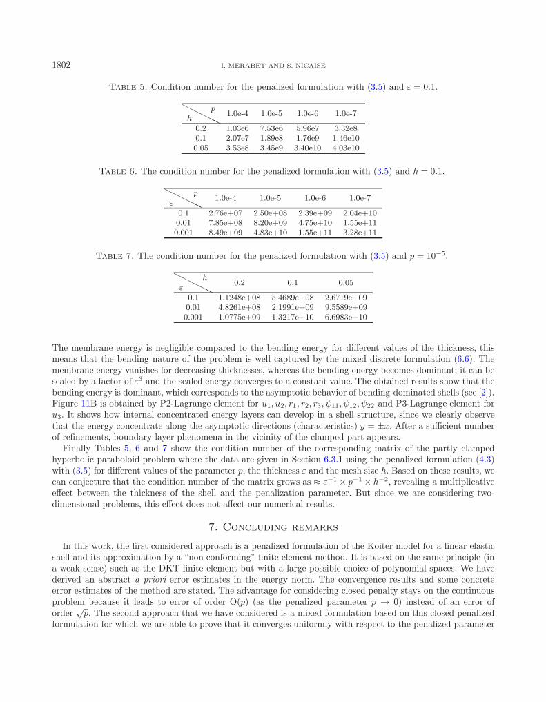
Table 5. Condition number for the penalized formulation with (3.5) and ε = 0.1.

��hp

1.0e-4 1.0e-5 1.0e-6 1.0e-7

0.2 1.03e6 7.53e6 5.96e7 3.32e80.1 2.07e7 1.89e8 1.76e9 1.46e100.05 3.53e8 3.45e9 3.40e10 4.03e10

Table 6. The condition number for the penalized formulation with (3.5) and h = 0.1.

��εp

1.0e-4 1.0e-5 1.0e-6 1.0e-7

0.1 2.76e+07 2.50e+08 2.39e+09 2.04e+100.01 7.85e+08 8.20e+09 4.75e+10 1.55e+110.001 8.49e+09 4.83e+10 1.55e+11 3.28e+11

Table 7. The condition number for the penalized formulation with (3.5) and p = 10−5.

��εh

0.2 0.1 0.05

0.1 1.1248e+08 5.4689e+08 2.6719e+090.01 4.8261e+08 2.1991e+09 9.5589e+090.001 1.0775e+09 1.3217e+10 6.6983e+10

The membrane energy is negligible compared to the bending energy for different values of the thickness, thismeans that the bending nature of the problem is well captured by the mixed discrete formulation (6.6). Themembrane energy vanishes for decreasing thicknesses, whereas the bending energy becomes dominant: it can bescaled by a factor of ε3 and the scaled energy converges to a constant value. The obtained results show that thebending energy is dominant, which corresponds to the asymptotic behavior of bending-dominated shells (see [2]).Figure 11B is obtained by P2-Lagrange element for u1, u2, r1, r2, r3, ψ11, ψ12, ψ22 and P3-Lagrange element foru3. It shows how internal concentrated energy layers can develop in a shell structure, since we clearly observethat the energy concentrate along the asymptotic directions (characteristics) y = ±x. After a sufficient numberof refinements, boundary layer phenomena in the vicinity of the clamped part appears.

Finally Tables 5, 6 and 7 show the condition number of the corresponding matrix of the partly clampedhyperbolic paraboloid problem where the data are given in Section 6.3.1 using the penalized formulation (4.3)with (3.5) for different values of the parameter p, the thickness ε and the mesh size h. Based on these results, wecan conjecture that the condition number of the matrix grows as ≈ ε−1 × p−1 × h−2, revealing a multiplicativeeffect between the thickness of the shell and the penalization parameter. But since we are considering two-dimensional problems, this effect does not affect our numerical results.

7. Concluding remarks

In this work, the first considered approach is a penalized formulation of the Koiter model for a linear elasticshell and its approximation by a “non conforming” finite element method. It is based on the same principle (ina weak sense) such as the DKT finite element but with a large possible choice of polynomial spaces. We havederived an abstract a priori error estimates in the energy norm. The convergence results and some concreteerror estimates of the method are stated. The advantage for considering closed penalty stays on the continuousproblem because it leads to error of order O(p) (as the penalized parameter p → 0) instead of an error oforder

√p. The second approach that we have considered is a mixed formulation based on this closed penalized

formulation for which we are able to prove that it converges uniformly with respect to the penalized parameter


and the mesh size; hence this method is robust with respect to p. Indeed, if the bilinear form (3.5) is used(which leads to non closed penalization), the error deteriorates as p goes to zero. Another advantage of theproposed method is the fact that we can use very simple elements (in our numerical experiments we have usedP2 Lagrange elements for both displacement and rotation unknowns). This approach has been illustrated withgood numerical results.

For Koiter’s model, membrane locking can occur when the thickness goes to zero, its approximation byrobust and accurate mixed finite element methods was considered in [1,10,25]. We have proposed a “‘penalized-mixed” method and have tested it for the partly clamped hyperbolic paraboloid shell problem. This is a bendingdominated benchmark problem that allows to test whether a finite element procedure locks or not ([22]). Atleast for the chosen benchmark (Sect. 6.3), we have seen that combining the two techniques lead to a robustmethod in the sense that it does not suffer from the “membrane locking”. A rigorous analysis of this new methodis postponed to future works.

References

[1] D.N. Arnold and F. Brezzi, Locking-free finite element method for shells. Math. Comput. 66 (1997) 1–14.

[2] F. Auricchio, L. Beirao da Veiga and C. Lovadina, Remarks on the asymptotic behaviour of koiter shells. Comput. Struct. 80(2002).

[3] I. Babuska, The finite element method with penalty. Math. Comput. 27 (1973) 221–228.

[4] M. Bernadou, Methode d’elements finis pour les problemes de coques minces. Dunod (1994).

[5] C. Bernardi, A. Blouza, F. Hecht and H. Le Dret, A posteriori analysis of finite element discretizations of a Naghdi shell model.IMA. J. Numer. Anal. 33 (2013) 190–211.

[6] A. Blouza, L. El Alaoui and S. Mani−Aouadi, A posteriori analysis of penalized and mixed formulations of Koiter’s shellmodel. J. Comput. Appl. Math. 296 (2016) 138–155.

[7] A. Blouza and H. Le Dret, Existence and uniqueness for the linear Koiter shell model with little regularity. Quarterly Appl.Math. 57 (1999) 317–338.

[8] A. Blouza, F. Hecht and H. Le Dret, Two finite element approximations of Naghdi’s shell model in Cartesian coordinates.SIAM J. Numer. Anal. 44 (2006) 636–654.

[9] K.-J. Bathe and L.-W. Ho, A simple and effective element for analysis of general shell structures. Comput. Struct. 13 (1981).

[10] J.H. Bramble and T. Sun, A locking-free finite element method for Naghdi shells. J. Comput. Appl. Math. 89 (1997) 119–133.

[11] S.C. Brenner and L.R. Scott, The Mathematical Theory of Finite Element Methods. Springer Verlag, New York (2008).

[12] H. Brezis, Analyse fonctionnelle, Theorie et applications. Mathematiques Appliquees pour la Maıtrise. Masson, Paris (1983).

[13] D. Chapelle and R. Stenberg, Stabilized finite element formulations for shells in a bending dominated state. SIAM J. Numer.Anal. 36 (1998) 32–73.

[14] Ph.G. Ciarlet, The Finite Element Method for Elliptic Problems. Studies in Mathematics and its Applications. North-HollandAmsterdam (1978).

[15] Ph.G. Ciarlet, Mathematical elasticity. Theory of shells. III. Vol. 29 of Studies in Mathematics and its Applications. North-Holland Publishing Co., Amsterdam (2000).

[16] M. Dauge and E. Faou, Koiter estimate revisited. Math. Models Methods Appl. Sci. 20 (2010) 1–42.

[17] F. Hecht, New development in freefem++. J. Numer. Math. 20 (2010) 251–265.

[18] J. Pitkaranta, Y. Leino, O. Ovaskainen and J. Piila, Shell deformation states and the finite element method: a benchmarkstudy of cylindrical shells. Comput. Methods Appl. Mech. Eng. 181 (1995) 81–121.

[19] W.T. Koiter, On the foundations of the linear theory of thin elastic shells. Number B73 in Wetensch. Proc. Kon. Ned. Akad(1970).

[20] J.L. Lions. Quelques methodes de resolution des problemes aux limites non lineaires. Dunod-Gauthier-Viltars Paris (1969).

[21] G.M. Lindberg, M.D. Olson and G.R. Cowper, New developments in the finite element analysis bf shells. Ouart. Bull. Div.Mech. Comput. 4 (1969).

[22] P.-S. Lee and K-J. Bathe, On the asymptotic behavior of shell structures and the evaluation in finite element solutions. Comput.Struct. 80 (2002).

[23] B. Maury, Numerical analysis of finite element/volume penalty method. SIAM J. Numer. Anal. 47 (2009) 1126–1148.

[24] P.M. Naghdi, Foundations of elastic shell theory. In Vol. IV of Progress in Solid Mechanics. North-Holland, Amsterdam (1963)1–90.

[25] T. Sun, A locking-free mixed finite element method for the Koiter shell model. In Proc. of The 3rd IMACS Inter. Symp.Iterative Methods Sci. Comput. Edited by Jackson Hole. Wyoming (1977) 307–312.

a penalty method for a linear koiter shell model

Documents