A Physical Approach to Large-scaleStructure and Galaxy Formation

Malcolm Longair

Cavendish LaboratoryUniversity of Cambridge.

1

The Physics of Large-scale Structureand Galaxy Formation

In the second lecture, I will focus on the physics of the development of perturbations inthe standard picture and temperature fluctuations in the Cosmic Microwave BackgroundRadiation.

• Jeans’ Instability in the Expanding Universe

• The Development of the Standard Picture

• The Evolution of the Power-spectrum

• Physics of Fluctuations in the Cosmic Microwave Background Radiation

• Cosmological Parameters Revisited

2

The Object of the Exercise

The aim of the cosmologist is to explain how large-scale structures formed in theexpanding Universe in the sense that, if δ is the enhancement in density of someregion over the average background density , the density contrast ∆ = δ/ reachedamplitude 1 from initial conditions which must have been remarkably isotropic andhomogeneous. Once the initial perturbations have grown in amplitude to∆ = δ/ ≈ 1, their growth becomes non-linear and they rapidly evolve towardsbound structures in which star formation and other astrophysical process lead to theformation of galaxies and clusters of galaxies as we know them (see Lecture 3).

The density contrasts ∆ = δ/ for galaxies, clusters of galaxies and superclusters atthe present day are about ∼ 106, 1000 and a few respectively. Since the averagedensity of matter in the Universe changes as (1 + z)3, it follows that typical galaxiesmust have had ∆ = δ/ ≈ 1 at a redshift z ≈ 100. The same argument applied toclusters and superclusters suggests that they could not have separated out from theexpanding background at redshifts greater than z ∼ 10 and 1 respectively.

3

The Wave Equation for the Growthof Small Density Perturbations

The standard equations of gas dynamics for a fluid in a gravitational field consist ofthree partial differential equations which describe (i) the conservation of mass, or theequation of continuity, (ii) the equation of motion for an element of the fluid, Euler’sequation, and (iii) the equation for the gravitational potential, Poisson’s equation.

Equation of Continuity :∂

∂t+ ∇ · (v) = 0 ; (1)

Equation of Motion :∂v

∂t+ (v · ∇)v = −1

∇p −∇φ ; (2)

Gravitational Potential : ∇2φ = 4πG . (3)

These equations describe the dynamics of a fluid of density and pressure p in whichthe velocity distribution is v. The gravitational potential φ at any point is given byPoisson’s equation in terms of the density distribution .

The partial derivatives describe the variations of these quantities at a fixed point inspace. This coordinate system is often referred to as Eulerian coordinates.

4

The Wave Equation for the Growthof Small Density Perturbations

We perturb the system about the uniform expansion v = H0r:

v = v0 + δv, = 0 + δ, p = p0 + δp, φ = φ0 + δφ . (4)

After a bit of algebra, we find the following equation for the peculiar velocity induced bythe growth of the perturbation:

d

dt

(

δ

0

)

=d∆

dt= −∇ · δv , (5)

where ∆ = δ/0 is the density contrast. After much further algebra, we obtain thewave equation for ∆

d2∆

dt2+ 2

(

a

a

)

d∆

dt= ∆(4πG0 − k2c2s) , (6)

where the adiabatic sound speed c2s is given by ∂p/∂ = c2s and k is the properwavevector.

5

The Jeans’ Instability

The differential equation for gravitational instability in a static medium is obtained bysetting a = 0 . Then, for waves of the form ∆ = ∆0 exp i(k · r − ωt), the dispersionrelation,

ω2 = c2sk2 − 4πG0 , (7)

is obtained.

• If c2sk2 > 4πG0, the right-hand side is positive and the perturbations areoscillatory, that is, they are sound waves in which the pressure gradient is sufficientto provide support for the region. Writing the inequality in terms of wavelength,stable oscillations are found for wavelengths less than the critical Jeans’wavelength λJ

λJ =2π

kJ= cs

(

π

G

)1/2

. (8)

6

The Jeans’ Instability

• If c2sk2 < 4πG0, the right-hand side of the dispersion relation is negative,corresponding to unstable modes. The solutions can be written

∆ = ∆0 exp(Γt + ik · r) , (9)

where

Γ = ±[

4πG0

(

1 − λ2J

λ2

)]1/2

. (10)

The positive solution corresponds to exponentially growing modes. Forwavelengths much greater than the Jeans’ wavelength, λ ≫ λJ, the characteristicgrowth time for the instability is

τ = Γ−1 = (4πG0)−1/2 ∼ (G0)

−1/2 . (11)

This is the famous Jeans’ Instability and the time scale τ is the typical collapsetime for a region of density 0.

7

The Jeans’ Instability in an Expanding Medium

We return first to the full version of the differential equation for ∆.

d2∆

dt2+ 2

(

a

a

)

d∆

dt= ∆(4πG − k2c2s) . (12)

The second term 2(a/a)(d∆/dt) modifies the classical Jeans’ analysis in crucialways. It is apparent from the right-hand side of (12) that the Jeans’ instability criterionapplies in this case also but the growth rate is significantly modified. Let us work out thegrowth rate of the instability in the long wavelength limit λ ≫ λJ, in which case we canneglect the pressure term c2sk2. We therefore have to solve the equation

d2∆

dt2+ 2

(

a

a

)

d∆

dt= 4πG0∆ . (13)

Let us first consider the special cases Ω0 = 1 and Ω0 = 0 for which the scalefactor-cosmic time relations are

a = (32H0t)2/3 and a = H0t (14)

respectively.

8

The Jeans’ Instability in an Expanding Medium

The Einstein–de Sitter Critical Model Ω0 = 1. In this case,

4πG =2

3t2and

a

a=

2

3t. (15)

and we find the key result

∆ =δ

∝ (1 + z)−1 . (16)

In contrast to the exponential growth found in the static case, the growth of theperturbation in the case of the critical Einstein–de Sitter universe is algebraic. The

Empty, Milne Model Ω0 = 0 In this case,

= 0 anda

a=

1

t, (17)

and ∆ = constant.

In the early stages of the matter-dominated phase, the dynamics of the world modelstend to a ∝ t2/3, and the density contrast grows linearly with a. At redshifts Ω0z ≪ 1,the amplitudes of the perturbations grow very slowly.

9

The General Solutions

A general solution for the growth of the density contrast with scale-factor for allpressure-free Friedman world models can be rewritten in terms of the densityparameter Ω0 as follows:

d2∆

dt2+ 2

(

a

a

)

d∆

dt=

3Ω0H20

2a−3∆ , (18)

where, in general,

a = H0

[

Ω0

(

1

a− 1

)

+ ΩΛ(a2 − 1) + 1

]1/2. (19)

The solution for the growing mode can be written as follows:

∆(a) =5Ω0

2

(

1

a

da

dt

)∫ a

0

da′(

da′

dt

)3, (20)

where the constants have been chosen so that the density contrast for the standardcritical world model with Ω0 = 1 and ΩΛ = 0 has unit amplitude at the present epoch,a = 1. With this scaling, the density contrasts for all the examples we will considercorrespond to ∆ = 10−3 at a = 10−3. It is simplest to carry out the calculationsnumerically for a representative sample of world models.

10

Models with ΩΛ = 0

The development of densityfluctuations from a scale factora = 1/1000 to a = 1 are shownfor a range of world models withΩΛ = 0. These results areconsistent with the calculationscarried out above, in which it wasargued that the amplitudes of thedensity perturbations vary as∆ ∝ a so long as Ω0z ≫ 1, butthe growth essentially stops atsmaller redshifts.

11

Models with finite ΩΛ

The models of greatest interest are theflat models for which (Ω0 +ΩΛ) = 1,in all cases, the fluctuations havingamplitude ∆ = 10−3 at a = 10−3.The growth of the density contrast issomewhat greater in the cases Ω0 =0.1 and 0.3 as compared with thecorresponding cases with ΩΛ = 0.The fluctuations continue to grow togreater values of the scale-factor a,corresponding to smaller redshifts, ascompared with the models withΩΛ = 0.

12

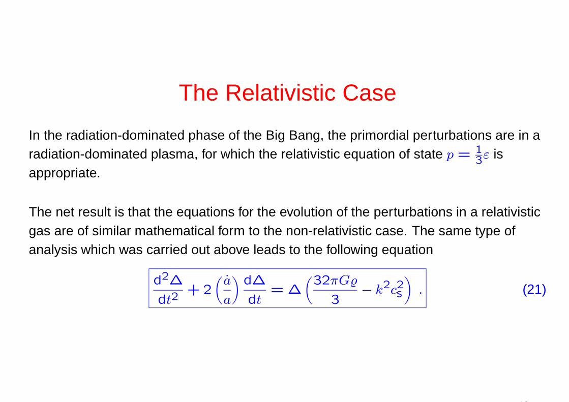
The Relativistic Case

In the radiation-dominated phase of the Big Bang, the primordial perturbations are in aradiation-dominated plasma, for which the relativistic equation of state p = 1

3ε isappropriate.

The net result is that the equations for the evolution of the perturbations in a relativisticgas are of similar mathematical form to the non-relativistic case. The same type ofanalysis which was carried out above leads to the following equation

d2∆

dt2+ 2

(

a

a

)

d∆

dt= ∆

(

32πG

3− k2c2s

)

. (21)

13

The Relativistic Case

The relativistic expression for the Jeans’ length is found by setting the right-hand sideequal to zero,

λJ =2π

kJ= cs

(

3π

8G

)1/2

, (22)

where cs = c/√

3 is the relativistic sound speed. The result is similar to the standardexpression for the Jeans’ length.

Neglecting the pressure gradient terms in (21), the following differential equation for thegrowth of the instability is obtained

d2∆

dt2+ 2

(

a

a

)

d∆

dt− 32πG

3∆ = 0 . (23)

In the radiation-dominated phases, the scale factor-cosmic time relation is given bya ∝ t1/2. Hence, for wavelengths λ ≫ λJ, the growing solution corresponds to

∆ ∝ t ∝ a2 ∝ (1 + z)−2 . (24)

Thus, once again, the unstable mode grows algebraically with cosmic time.

14

The Basic Problem of Structure Formation

Let us summarise the implications of the key results derived above. Throughout thematter- dominated era, the growth rate of perturbations on physical scales muchgreater than the Jeans’ length is

∆ =δ

∝ a =

1

1 + z. (25)

Since galaxies and astronomers certainly exist at the present day z = 0, it follows that∆ ≥ 1 at z = 0 and so, at the last scattering surface, z ∼ 1,000, fluctuations musthave been present with amplitude at least ∆ = δ/ ≥ 10−3.

• The slow growth of density perturbations is the source of a fundamental problem inunderstanding the origin of galaxies – large-scale structures did not condense outof the primordial plasma by exponential growth of infinitesimal statisticalperturbations.

• Because of the slow development of the density perturbations, we have theopportunity of studying the formation of structure on the last scattering surface at aredshift z ∼ 1,000.

15

Summary of the Thermal History of the Universe

This diagram summarises the keyepochs in the thermal history of theUniverse. The key epochs are

• The epoch of recombinationz = 1000.

• The epoch of equality of matterand radiation, includingneutrinos, z = 3530.

16

The Sound Speed as a Function of Cosmic Epoch

The speed of sound cs is given by

c2s =

(

∂p

∂

)

S

, (26)

where the subscript S means ‘at constant entropy’, that is, adiabatic sound waves. Thedominant contributors to p and change dramatically as the Universe changes frombeing radiation- to matter-dominated. The sound speed can then be written

c2s =(∂p/∂T)r

(∂/∂T)r + (∂/∂T)m, (27)

where the partial derivatives are taken at constant entropy. This reduces to thefollowing expression:

c2s =c2

3

4r

4r + 3m. (28)

Thus, in the radiation-dominated era, the speed of sound tends to the relativistic soundspeed, cs = c/

√3.

17

The Damping of Sound Waves

Although the matter and radiation are closely coupled throughout the pre-recombinationera, the coupling is not perfect and radiation can diffuse out of the densityperturbations. Since the radiation provides the restoring force for support for theperturbation, the perturbation is damped out if the radiation has time to diffuse out of it.This process is often referred to as Silk damping.

At any epoch, the mean free path for scattering of photons by electrons isλ = (NeσT)−1, where σT = 6.665 × 10−29 m2 is the Thomson cross-section. Thedistance which the photons can diffuse is

rD ≈ (Dt)1/2 =(

13λct

)1/2, (29)

where t is cosmic time. The baryonic mass within this radius, MD = (4π/3)r3DB, cannow be evaluated for the pre-recombination era.

18

The Particle Horizon

One of the key concepts is that of particle horizons. At any epoch t, the particle horizonis defined to be the maximum distance over which causal communication could havetaken place by that epoch. In other words, this distance describes how far a light signalcould have travelled from the origin of the Big Bang at t = 0 by the epoch t.

The radial comoving distance coordinate r corresponding to the distance travelled by alight signal from the origin of the Big Bang to the epoch t is

r =

∫ t

0

cdt

a(t)=

∫ z

∞(1 + z)cdt . (30)

To find the horizon scale at the epoch corresponding to redshift z, we simply scale r bythe scale factor a(t) = (1 + z)−1. Thus, the definition of the particle horizon rH(t) atthe cosmic epoch t, corresponding to the redshift z is

rH(t) = a(t)∫ t

0

cdt

a(t)=

1

1 + z

∫ z

∞(1 + z)cdt . (31)

19

Horizons

At early times, all the Friedman models tend toward the dynamics of the critical modeland the particle horizon becomes rH(t) = 3ct. This make physical sense since onemight expect that the typical distance which light could travel by the epoch t would be oforder ct. The factor 3 takes account of the fact that fundamental observers were closertogether at early epochs and so greater distances could be causally connected than ct.A similar calculation can be carried out for the radiation-dominated era and then we findrH(t) = 2ct.

Equally important is the Hubble sphere. This is the distance at which v = c accordingto Hubble’s law v = Hr at any epoch, where H = a/a. This is the distance over whichcausal phenomena can take place at a particular epoch. We will have a lot to say aboutthe Hubble sphere in the first pedagogical lecture.

20

The Simple Baryonic Picture

We can put together all these ideasto develop the simplest picture ofgalaxy formation. This is thesimplest baryonic picture. Itincludes many of the featureswhich will reappear in the ΛCDMpicture. The diagram shows howthe horizon mass MH, the Jeansmass MJ and the Silk Mass MD

change with scale factor a.

21

The Simple Baryonic Picture

This diagrams, from Coles andLucchin (1995) showsschematially how structuredevelops in a purely baryonicUniverse. The problem is thatthe temperature fluctuations onthe last scattering surface asexpected to be at least∆T/T ∼ 10−3, far in excess ofthe observed limits.The solution to this problemcame with the realisation thatthe dark matter is the dominantcontribution to Ω0.

22

Dark Matter

There is no question but that the Universe is dominated gravitationally on small scalesby Dark Matter.

These reconstructions of the total mass distribution from gravitational lensing show thatthe dark matter is dynamically dominant in clusters of galaxies.

23

Instabilities in the Presence of Dark Matter

Neglecting the internal pressure of the fluctuations, the expressions for the densitycontrasts in the baryons and the dark matter, ∆B and ∆D respectively, can be writtenas a pair of coupled equations

∆B + 2

(

a

a

)

∆B = AB∆B + AD∆D , (32)

∆D + 2

(

a

a

)

∆D = AB∆B + AD∆D . (33)

Let us find the solution for the case in which the dark matter has Ω0 = 1 and thebaryon density is negligible compared with that of the dark matter. Then (33) reduces tothe equation for which we have already found the solution ∆D = Ba where B is aconstant. Therefore, the equation for the evolution of the baryon perturbations becomes

∆B + 2

(

a

a

)

∆B = 4πGDBa . (34)

24

Instabilities in the Presence of Dark Matter

Since the background model is the critical model, equation (34) simplifies to

a3/2 d

da

(

a−1/2d∆

da

)

+ 2d∆

da= 3

2B . (35)

The solution, ∆ = B(a − a0), satisfies (35). This result has the following significance.Suppose that, at some redshift z0, the amplitude of the baryon fluctuations is verysmall, that is, very much less than that of the perturbations in the dark matter. Theabove result shows how the amplitude of the baryon perturbation developssubsequently under the influence of the dark matter perturbations. In terms of redshiftwe can write

∆B = ∆D

(

1 − z

z0

)

. (36)

Thus, the amplitude of the perturbations in the baryons grows rapidly to the sameamplitude as that of the dark matter perturbations. The baryons fall into the dark matterperturbations and rapidly attain amplitudes the same as those of the dark matter.

25

The Cold Dark Matter Picture

This diagram shows how structuredevelops in a cold dark matterdominated Universe. Theamplitudes of the baryonicperturbations were very muchsmaller than those in the cold darkmatter at the epoch ofrecombination.

Note also the origin of the Acousticor Sakharov peaks in the predictedmass spectrum (from Sunyaev andZeldovich 1970).

This is the favoured model for theformation structure.

26

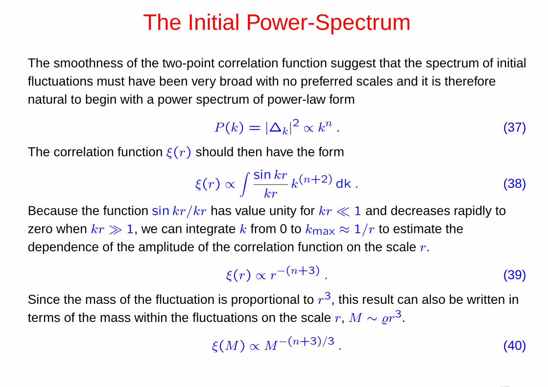
The Initial Power-Spectrum

The smoothness of the two-point correlation function suggest that the spectrum of initialfluctuations must have been very broad with no preferred scales and it is thereforenatural to begin with a power spectrum of power-law form

P(k) = |∆k|2 ∝ kn . (37)

The correlation function ξ(r) should then have the form

ξ(r) ∝∫

sin kr

krk(n+2) dk . (38)

Because the function sin kr/kr has value unity for kr ≪ 1 and decreases rapidly tozero when kr ≫ 1, we can integrate k from 0 to kmax ≈ 1/r to estimate thedependence of the amplitude of the correlation function on the scale r.

ξ(r) ∝ r−(n+3) . (39)

Since the mass of the fluctuation is proportional to r3, this result can also be written interms of the mass within the fluctuations on the scale r, M ∼ r3.

ξ(M) ∝ M−(n+3)/3 . (40)

27

The Initial Power-Spectrum

Finally, to relate ξ to the root-mean-square density fluctuation on the mass scale M ,∆(M), we take the square root of ξ, that is,

∆(M) =δ

(M) = 〈∆2〉1/2 ∝ M−(n+3)/6 . (41)

This spectrum has the important property that the density contrast ∆(M) had thesame amplitude on all scales when the perturbations came through their particlehorizons. Let us illustrate how this comes about.

Before the perturbations came through their particle horizons and before the epoch ofequality of matter and radiation energy densities, the density perturbations grew as∆(M) ∝ a2, although the perturbation to the gravitational potential was frozen-in.Therefore, the development of the spectrum of density perturbations can be written

∆(M) ∝ a2 M−(n+3)/6 . (42)

28

The Initial Power-Spectrum

A perturbation of scale r came through the horizon when r ≈ ct, and so the mass ofdark matter within it was MD ≈ D(ct)3. During the radiation dominated phases,a ∝ t1/2 and the number density of dark matter particles, which will eventually formbound structures at z ∼ 0, varied as ND ∝ a−3.

Therefore, the horizon dark matter mass increased as MH ∝ a3, or, a ∝ M1/3H . The

mass spectrum ∆(M)H when the fluctuations came through the horizon at differentcosmic epochs was

∆(M)H ∝ M2/3 M−(n+3)/6 = M−(n−1)/6 . (43)

Thus, if n = 1, the density perturbations ∆(M) = δ/(M) all had the sameamplitude when they came though their particle horizons during theradiation-dominated era.

29

The Harrison–Zeldovich Power Spectrum, n = 1

The scale-independence of the density perturbations, δ/ = 10−4 was derived fromthe analysis of Sunyaev and Zeldovich who used a variety of constraints to derive theform of the initial power-spectrum of density perturbations as they came through thehorizon on mass scales from 105 to 1020 M⊙.

Harrison’s paper addressed the form the primordial spectrum would have to have inorder to prevent the overproduction of excessively large amplitude perturbations onsmall and large scales. If the spectral index were greater than n = 1, there would havebeen excessively large metric perturbations on very small scales in the early Universewhich would inevitably have resulted in their collapse to form black holes. The n = 1

spectrum does not diverge on large physical scales and so is consistent with theobserved large-scale isotropy of the Universe.

30

Processing of the Initial Power Spectrum

We do not observe the initial power-spectrum except on the largest physical scales.The transfer function T(k) which describes how the shape of the initial power-spectrum∆k(z) in the dark matter is modified by different physical processes through therelation

∆k(z = 0) = T(k) f(z)∆k(z) . (44)

∆k(z = 0) is the power spectrum at the present epoch and f(z) ∝ a ∝ t2/3 is thelinear growth factor between the scale factor at redshift z and the present epoch in thematter dominated era.

The form of the transfer function is largely determined by the fact that there is a delay inthe growth of the perturbations between the time when they came through the horizonand began to grow again. In the standard baryonic picture, this is associated with thefact that before the epoch of equality of matter and radiation, the oscillations in thephoton-baryon plasma were dynamically more important than those in the dark matter.

31

The Processed Harrison–Zeldovich Power Spectrum

Notice that on very large scales (small wavenumbers) the spectrum is unprocessed. Onthe scale of galaxies and clusters, the spectrum has been strongly modified.

32

The Processed Harrison–Zeldovich Power SpectrumAdding in the Baryons

Four examples of the transfer functionsfor models of structure formation withbaryons only (top pair of diagrams) andwith mixed cold and baryonic models(bottom pair of diagrams) by Eisensteinand Hu. The numerical results are shownas solid lines and their fitting functions bydashed lines. The lower small boxes ineach diagram show the percentageresiduals to their fitting functions, whichare always less than 10%.

The evidence for these perturbations inthe distribution of galaxies was shown inthe first lecture.

33

The Acoustic Oscillations in the Galaxy Distribution

AAT 2dF galaxy survey

SDSS galaxy survey

34

The Basic Input Parameters for the Models

• Selection of a cosmological model with values of Ω0, ΩΛ and H0.

• The ordinary baryonic matter has density parameter ΩB, which is only about5-10% of the dark matter.

• The power-spectrum of the initial perturbations is assumed to be ofHarrison-Zeldovich form p(k) = Akn with random phases. The value of n can bevaried to find the best fit to the observations.

The computational physicists can, however, include many more variables as shown onthe next slide.

35

• h = (H0/100 km s−1 Mpc−1)

• ωb = Ωbh2, the baryon density parameter

• ωd = Ωdh2 dark matter density parameter

• ΩΛ = dark energy density parameter

• w = dark energy equation of state, p = wρc2 (w = −1 ”prefered”)

• τ = reionisation optical depth

• ΩK = space curvature, recalling that Ωm + ΩΛ + ΩK = 1

• As = amplitude of scalar power-spectrum

• ns = scalar spectral index; ns = 1 preferred

• a = running of scalar spectral index

• r = tensor-scalar ratio

• nt = tensor spectral index

• b = bias factor

• fn = neutrino fraction Show simulations

36

Fluctuations in the Cosmic MicrowaveBackground Radiation

We now need to relate the perturbations in the dark matter, the radiation and thebaryons to what is expected to be observed in the intensity and polarisation of theCosmic Microwave Background Radiation. A key result concerns the thickness of thelayer from which the photons of the CMB were last scattered.

The ionisation fraction xe = Ne/NH asa function of redshift z for theconcordance set of cosmologicalparameters.

The visibility function

v(z) = e−τ dτ/dz

describes the probability of the photonswe observe being scattered at differentredshifts.

37

Perturbations on the Last Scattering Layer

The diagram shows schematicallythe size of various smallperturbations compared with thethickness of the last scatteringlayer. On very large scales, theperturbations are very much largerthan the thickness of the layer. Onscales less than clusters ofgalaxies, many perturbationsoverlap, reducing the amplitude ofthe perturbations.

38

Large Angular Scales - the Sachs-Wolfe Effect

On the very largest scales, the dominant source of intensity fluctuations results from thefact that the photons we observe have to climb out of the gravitational potential wellsassociated with perturbations which are very much greater in size than the thickness ofthe last scattering layer.

On the scales of interest, the fluctuations at the epoch of recombination far exceed thehorizon scale and so the perturbations would represent a change of the gravitationalpotential of everything within the horizon. More properly, we should describe theseperturbations as metric perturbations. These ‘super-horizon’ perturbations raise thethorny question of the choice of gauge to be used in relativistic perturbation theory. Ageneral relativistic treatment, first performed by Sachs and Wolfe (1967), is needed.The result is ∆T/T = (1/3)∆φ/c2, recalling that ∆φ is a negative quantity.

39

The Sachs-Wolfe EffectThe Coles-Lucchin Argument

Coles and Lucchin (1995) rationalised how the Sachs–Wolfe answer can be found. Inaddition to the Newtonian gravitational redshift, because of the perturbation of themetric, the cosmic time, and hence the scale factor a, at which the fluctuations areobserved, are shifted to slightly earlier cosmic times. Temperature and scale factorchange as ∆T/T = −∆a/a. For all the standard models in the matter-dominatedphase a ∝ t2/3 and so the increment of cosmic time changes as ∆a/a = (2/3)∆t/t.

But ∆ν/ν = −∆t/t is just the Newtonian gravitational redshift, with net result thatthere is a positive contribution to ∆T/T of −(2/3)∆φ/c2. The net temperaturefluctuation is ∆T/T = 1

3∆φ/c2.

It is then a straightforward calculation to show that, for the Ω0 = 1 model, thetemperature fluctuations depend upon angular scale as

∆T

T≈ 1

3

∆φ

c2∝ θ(1−n)/2 . (45)

40

The Power Spectrum of the Fluctuationsin the Cosmic Microwave Background Radiation

For the preferred Harrison-Zeldovichspectrum n = 1, we expect the powerspectrum to be independent of angle onlarge angular scales. The flatness of thepower spectrum on large angular scaleswas discovered by COBE and fullyconfirmed by the power spectrumobtained by the Wilkinson MicrowaveAnisotropy Probe (WMAP). The detailedshape on large angular scales dependsupon the choice of cosmological model.

41

Intermediate Angular Scales

In the case of Cold Dark Matter, all scales are unstable and grow according to thestandard formula from the time they become dynamically dominant.

• We need the Jean’s length of the photon-dominated plasma at the epoch ofrecombination. For the concordance values of the cosmic parameters, the inertia inthe baryonic matter is more or less the same as the inertial mass in the radiation atthe epoch of recombination. Therefore, the appropriate sound speed to use is veryclose to c/

√6 and

λs =c√6

t =7 × 1020

(Ω0h2)m , (46)

This scale corresponds to a comoving length scale of 32.5(ΩBh2)−1 ≈ 200 Mpc.

• Not surprisingly, this scale is the same as the sound horizon on the last scatteringsurface

λs = cst (47)

The importance of this result that this corresponds to the maximum wavelengthwhich the sound waves can have on the last scattering surface.

42

Intermediate Angular Scales

The first acoustic peak is associated with perturbations on the scale of the soundhorizon at the epoch of recombination. The amplitudes of the acoustic waves at the lastscattering layer depend upon the phase difference from the time they came through thehorizon to last scattering layer, that is, they depend upon

∫

dφ =

∫

ω dt . (48)

Let us label the wavenumber of the first acoustic peak k1. Oscillations which are nπ outof phase with the first acoustic peak also correspond to maxima in the temperaturepower spectrum at the epoch of recombination. There is, however, an importantdifference between the even and odd harmonics of k1. The odd harmonics correspondto the maximum compression of the waves and so to increases in the temperature,whereas the even harmonics correspond to rarefactions of the acoustic waves and soto temperature minima. The perturbations with phase differences π(n + 1

2) relative tothat of the first acoustic peak have zero amplitude at the last scattering layer andcorrespond to the minima in the power spectra.

43

Intermediate Angular Scales

To find the acoustic peaks, we need to find the wavelengths corresponding tofrequencies

ωtrec = nπ . (49)

Adopting the short wavelength dispersion relation ,

ω2 = c2sk2 − 4πGB = c2s(k2 − k2

J) ≈ c2sk2 , (50)

the condition becomes

cskntrec = nπ kn =nπ

λs= nk1 . (51)

Thus, the acoustic peaks are expected to be evenly spaced in wavenumber. Theseparation between the acoustic peaks thus provides us with further information aboutvarious combinations of cosmological parameters.

44

Intermediate Angular Scales

The next task is to determine the amplitudes of the acoustic peaks in the powerspectrum. The acoustic oscillations take place in the presence of growing densityperturbations in the dark matter, which have greater amplitude than those in theacoustic oscillations. Therefore, the acoustic waves are driven by the larger densityperturbations in the dark matter with the same wavelength, that is, the perturbations areforced oscillations. In a simple approximation, growth rate of the oscillation is driven bythe growing amplitude of the dark matter perturbations:

d2∆B

dt2= ∆D4πGρD − ∆Bk2c2s . (52)

The sound speed is given by

cs =c√3

(

4rad

4rad + 3B

)1/2

=c

√

3(1 + R), (53)

where R = 3B/4rad.

45

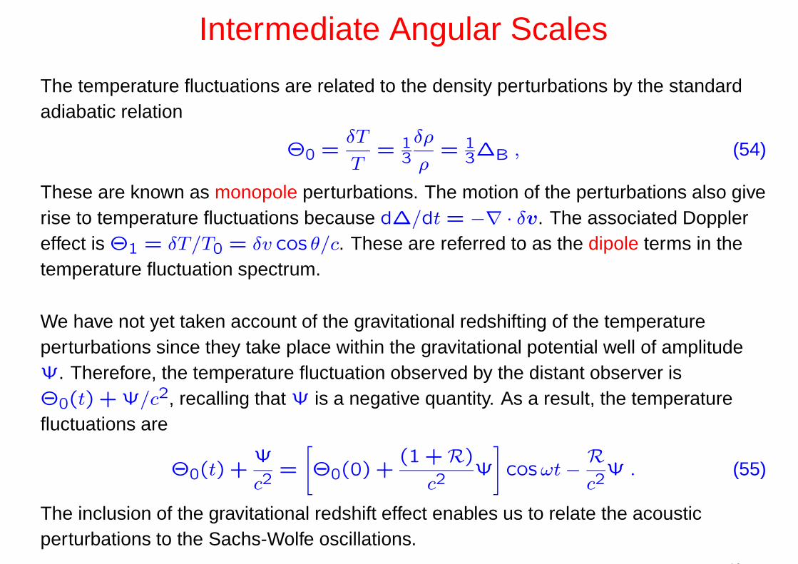
Intermediate Angular Scales

The temperature fluctuations are related to the density perturbations by the standardadiabatic relation

Θ0 =δT

T= 1

3

δρ

ρ= 1

3∆B , (54)

These are known as monopole perturbations. The motion of the perturbations also giverise to temperature fluctuations because d∆/dt = −∇ · δv. The associated Dopplereffect is Θ1 = δT/T0 = δv cos θ/c. These are referred to as the dipole terms in thetemperature fluctuation spectrum.

We have not yet taken account of the gravitational redshifting of the temperatureperturbations since they take place within the gravitational potential well of amplitudeΨ. Therefore, the temperature fluctuation observed by the distant observer isΘ0(t) + Ψ/c2, recalling that Ψ is a negative quantity. As a result, the temperaturefluctuations are

Θ0(t) +Ψ

c2=

[

Θ0(0) +(1 + R)

c2Ψ

]

cosωt − Rc2

Ψ . (55)

The inclusion of the gravitational redshift effect enables us to relate the acousticperturbations to the Sachs-Wolfe oscillations.

46

Intermediate Angular Scales

In the limit R → 0, the monopole and dipole temperature fluctuations are of the sameamplitude. However, when the inertia of the baryons can no longer be neglected, themonopole contribution becomes significantly greater than the dipole term.

At maximum compression, kλs = π, the amplitude of the observed temperaturefluctuation is (1 + 6R) times that of the Sachs–Wolfe effect. Furthermore, theamplitudes of the oscillations are asymmetric if R 6= 0, the temperature excursionsvarying between −(Ψ/c2)(1+6R) for kλs = (2n+1)π and (Ψ/c2) for kλs = 2nπ.

These results can account for the some of the prominent features of the temperaturefluctuation spectrum. The temperature perturbations associated with the acousticpeaks are much larger than the Sachs–Wolfe fluctuations. The asymmetry between theeven and odd peaks in the fluctuation spectrum is associated with the extracompression at the bottom of the gravitational potential wells when account is taken ofthe inertia of the perturbations associated with the baryonic matter.

47

Small Angular Scales

• Silk Damping scale results in the suppression of high wave number modes onscales less than about 8 Mpc at the present epoch.

• The superposition of perturbations damps out the perturbations within the lastscattering layer.

• The Sunyaev-Zeldovich effect associated with hot intergalactic gas in clusters ofgalaxies creates additional small scale perturbations.

48

The WMAP One-year Power Spectrum

Many of the features of the aboveanalysis can be observed in the WMAPpower spectrum.

• The location of the maximum of thefirst peak in the power spectrum.

• The asymmetry between the first,second and third peaks.

• The flatness of the spectrum at lowvalues of l.

• The polarisation and the largesignal at very small values of l.

49

Parameter Estimation using WMAP and SDSS

Max Tegmark and hiscolleagues used theone-year WMAPpower-spectrum andpolarisation to makeparameter estimates. Theyellow areas showprobability distributionsusing WMAP alone; thered areas include thepower spectrum ofgalaxies from the SloanDigital Sky Survey.

50

The Polarisation of the Cosmic MicrowaveBackground Radiation

The mechanism for creating polarisation of the Cosmic Microwave BackgroundRadiation is Thomson scattering of the radiation by free electrons. A beam ofunpolarised radiation incident upon a free electron causes it to oscillate in the planeperpendicular to the direction of the beam. The accelerated electron radiates with adipole pattern so that the scattered radiation is 100% polarised when the electron isviewed perpendicular to the direction of propagation of the beam.

In the case of the Cosmic Background Radiation, the distribution of the radiation ishighly isotropic and, in the case of complete isotropy, there would be exact cancellationof the polarised signals. Even in the case of a dipole distribution of the re-radiated field,there is no net polarisation because of the symmetry of the Thomson scatteringprocess. The only way of creating a net polarised signal is if the radiation field incidentupon the electron has a quadrupole anisotropic distribution of intensity.

51

The Polarisation of the CMBR

Zeldovich and Sunyaev argued that the detection of a polarised signal in the CosmicMicrowave Background Radiation would be evidence for a quadrupole component in itsintensity. For an incident radiation field

I = I0

1 + aµ + b

(

µ2 − 1

3

)

+∞∑

n=3

CnPn

, (56)

where µ = cos θ, the term in a corresponds to a dipole field and that in b to aquadrupole field. The Pns are higher order Legendre polynomials. Integrating over allangles of incidence of the incoming radiation, the fractional polarisation is

p =I‖ − I⊥I‖ + I⊥

= 0.1bµ2τ . (57)

where τ is the optical depth of the region for Thomson scattering. In theRayleigh-Jeans region of the spectrum, a, b and Cn are independent of frequency.Polarisation is a tensor quantity and so it is proportional to the quadrupole term butdoes not depend upon the dipole or higher terms in the intensity angular distribution.

52

Polarisation from the Last Scattering Layer

The radiation field seen by an electronin the last scattering later is anisotropicbecause of the Doppler shiftsassociated with the dipole term Θ1 inthe expression for the power-spectrumof temperature fluctuations. Theseresult in first-order temperatureperturbations ∆I/I = (v/c) cos θ andthese are the source of the quadrupoleintensity distribution. The diagramshows the predicted amplitude of theDoppler component compared withother contributions to the totalpower-spectrum.

53

Polarisation from the Last Scattering Layer

The important points to note are:

• The Doppler component is out of phase with the significantly larger monopolecomponent and its power spectrum decreases in amplitude with decreasingmultipole l. Coherent oscillations cannot exist on scales greater than the soundhorizon in the last scattering layer.

• The formation of the polarised signal involves two Thomson scattering events. Thefirst created the quadrupolar field through scattering from motions caused by theoscillating baryon perturbations and the second by scattering of the quadrupolarfield.

• The maximum of the polarised signal occurs at wavelengths which are of the sameorder as the mean free path of the photons in the last scattering layer.

54

The Three-year WMAP Polarisation Results

Plots for the total intensity, the polarisedintensity and the cross-correlationbetween the total intensity and thepolarised intensity are labelled TT, EEand TE respectively. The dashedsections of the TE curve indicatesmultipoles in which the polarisationsignal is anticorrelated with the totalintensity.

55

Polarisation from the Epoch of Reionisation

One of the exciting results of the WMAP data has been the presence of stronglypolarised signals in the TE cross-correlation power-spectrum at small multipoles . Thisis a signature of the epoch when the intergalactic gas was reheated and reionised. Thephysics of the generation of linearly polarised emission during reionisation is exactly thesame as that which resulted in the formation of polarisation in the last scattering layer.

Once the intergalactic gas was reionised, any quadrupolar component of thebackground radiation created a linearly polarised signal. The strongest signal is againexpected to occur at those multipoles for which the mean free path of the backgroundphotons is equal to the wavelength of the perturbations. It follows that, because asignificant coherent polarised signal is observed at low multipoles, the scattering mustoccur on large physical scales at rather late epochs. Also, the perturbations had grownin amplitude by the epoch of reionisation giving rise to a more strongly polarised signal.

56

Polarisation from the Epoch of Reionisation

The amplitude of the polarisation signalis determined by the optical depth τ ofthe intergalactic gas once it is reionised.The amplitude of the polarisation signalcan be predicted rather precisely foradiabatic perturbations once the initialpower-spectrum is given. The dipoleterm Θ1 is the cause of the quadrupolecomponent responsible for thegeneration of the linearly polarisedsignal. This procedure is repeated forthe late reionisation phases andaccounts for the predicted linearpolarisation ‘bump’ seen in the EE andTE power spectra.

57

The Properties of the Concordance Model

Adopting H0 = 73 km s−1 Mpc−1, we find the following self-consistent set ofparameters:

Hubble’s constant H0 = 73 km s−1 Mpc−1

Curvature of Space ΩΛ + Ω0 = 1

Baryonic density parameter ΩB = 0.04Cold Dark Matter density parameter ΩD = 0.24

Total Matter density parameter Ω0 = 0.28Density Parameter in Vacuum Fields ΩΛ = 0.72

Scalar spectral index ns = 0.961Optical Depth for Thomson Scattering on Reheating τ = 0.09

The one addition to the table is the scalar spectral index of the initial power spectrum,ns = 0.961+0.018

−0.019 . This may be evidence that there should be a detectable signatureat small multipoles for primordial gravitational waves. They would show up through theirB-mode polarisation signals, but this is a really tough experiment.

58

The Spectrum of the PrimordialGravitational Waves

The predicted power spectrum offluctuations in the Cosmic MicrowaveBackground Radiation due to scalarperturbations (density perturbations;top) and tensor perturbations (gravitywaves; bottom) for a tensor-to-scalarratio r = 1.

59