a platform for indoor localisation, mapping, and data ... · a platform for indoor localisation,...

A Platform for Indoor Localisation,Mapping, and Data Collection using an

Autonomous Vehicle

Andreas Teodor [email protected]

Oscar [email protected]

14th June 2017

Master’s thesis work carried out at Combain Mobile AB.

Supervisors: Rikard Windh, [email protected]örn Lindquist, [email protected] Åström, [email protected]

David Gillsjö, [email protected]

Examiner: Magnus Oskarsson, [email protected]

mailto:[email protected]







Abstract

Everyone who has worked with research knows how rewarding experiment-ing and developing new algorithms can be. However in some cases, the hardpart is not the invention of these algorithms, but their evaluation. To tryand make that evaluation easier, this thesis focuses on the collection of datathat can be used as positional ground truths using an autonomous measure-ment platform. This should assist Combain Mobile AB in the evaluation andimprovement of their Wi-Fi based indoor positioning service.

How and which parts of the open-source community’s work in the RobotOperating System (ROS) project to utilise is not obvious. This thesis there-fore sets out to build a Minimum Viable Product (MVP) which is capable ofsupporting two di�erent use cases: measure and explore inside an unknownenvironment, and measure inside a known environment given a map. Thise�ectively leaves Combain with a viable product, and indirectly helps thecommunity by aiding it in comparing and recommending the best tools andsoftware libraries for the task.

The result of this thesis ends up recommending the following for meas-uring inside an unknown environment: the Simultaneous Localisation AndMapping (SLAM) algorithm Google Cartographer for navigation, and theexploration algorithm Hector Exploration for planning the exploration. Tomeasure inside a known environment the following is recommended: theAdaptive Monte Carlo Localisation (AMCL) positioning algorithm and theSpanning Tree Covering algorithm.

Keywords: Area Coverage, Autonomous Vehicles, Exploration, Robotic OperatingSystem (ROS), SLAM, Wi-Fi

Acknowledgements

We would �rst like to extend our sincerest gratitude to our academic supervisors: Prof.Kalle Åström and Ph.D. student David Gillsjö at Lund University, Faculty of Engineering.Their extensive knowledge and experience has been an immense help in ensuring thesuccess of this thesis. We are grateful for the multiple in-depth discussions which haveinspired multiple ideas, and we would like to express our thanks for the encouragementand critique of this thesis.

We would also like to extend our gratitude to everyone at Combain Mobile ABfor allowing us to conduct our master’s thesis at their company and for providing aworkplace. Special thanks to Björn Lindquist and Rikard Windh for supervising thisthesis and providing many good suggestions. Huge thanks to Anders Mannesson forhelping us understand their existing indoor solution, his many in-depth reviews, and forlistening to us ramble on without actually having any o�cial role in this thesis.

This thesis builds upon the excellent work of the Robot Operating System community,which have our heartfelt thanks for making this thesis possible.

Last, we would like to thank our friends and families, whom have supported us duringboth this thesis, and the duration of our studies. We could not have done it without yoursupport!

3

Contents

Glossary 9

Acronyms 11

1 Introduction 131.1 Background . . . . . . . . . . . . . . . . . . . . . . . . . . . . . . . . . . 13

1.1.1 Purpose and Goal . . . . . . . . . . . . . . . . . . . . . . . . . . . 141.1.2 Use Cases . . . . . . . . . . . . . . . . . . . . . . . . . . . . . . . 15

1.2 Robot Operating System . . . . . . . . . . . . . . . . . . . . . . . . . . . 151.2.1 Navigation Stack . . . . . . . . . . . . . . . . . . . . . . . . . . . 15

1.3 Simulations . . . . . . . . . . . . . . . . . . . . . . . . . . . . . . . . . . . 161.4 Robot Hardware . . . . . . . . . . . . . . . . . . . . . . . . . . . . . . . . 16

1.4.1 Controller Unit . . . . . . . . . . . . . . . . . . . . . . . . . . . . 161.4.2 Sensors . . . . . . . . . . . . . . . . . . . . . . . . . . . . . . . . 17

1.5 Network . . . . . . . . . . . . . . . . . . . . . . . . . . . . . . . . . . . . 191.6 Related Work . . . . . . . . . . . . . . . . . . . . . . . . . . . . . . . . . . 191.7 Contribution . . . . . . . . . . . . . . . . . . . . . . . . . . . . . . . . . . 201.8 Disposition . . . . . . . . . . . . . . . . . . . . . . . . . . . . . . . . . . . 21

2 Methodology 232.1 Approach . . . . . . . . . . . . . . . . . . . . . . . . . . . . . . . . . . . . 23

2.1.1 Initial Research . . . . . . . . . . . . . . . . . . . . . . . . . . . . 242.1.2 Iterations . . . . . . . . . . . . . . . . . . . . . . . . . . . . . . . 242.1.3 Wrap-up . . . . . . . . . . . . . . . . . . . . . . . . . . . . . . . . 24

2.2 Simulated and Real World Trials . . . . . . . . . . . . . . . . . . . . . . . 242.3 Schedule . . . . . . . . . . . . . . . . . . . . . . . . . . . . . . . . . . . . 25

3 Simultaneous Localization And Mapping 273.1 Motivation . . . . . . . . . . . . . . . . . . . . . . . . . . . . . . . . . . . 273.2 OpenSlam’s Gmapping . . . . . . . . . . . . . . . . . . . . . . . . . . . . 27

5

CONTENTS

3.2.1 Impression . . . . . . . . . . . . . . . . . . . . . . . . . . . . . . . 283.2.2 Loop Closure . . . . . . . . . . . . . . . . . . . . . . . . . . . . . 28

3.3 Hector SLAM . . . . . . . . . . . . . . . . . . . . . . . . . . . . . . . . . 283.3.1 Impression . . . . . . . . . . . . . . . . . . . . . . . . . . . . . . . 30

3.4 Google Cartographer . . . . . . . . . . . . . . . . . . . . . . . . . . . . . 303.4.1 Impression . . . . . . . . . . . . . . . . . . . . . . . . . . . . . . . 303.4.2 Loop Closure . . . . . . . . . . . . . . . . . . . . . . . . . . . . . 30

3.5 Evaluation . . . . . . . . . . . . . . . . . . . . . . . . . . . . . . . . . . . 313.5.1 Loop Closure . . . . . . . . . . . . . . . . . . . . . . . . . . . . . 313.5.2 Accuracy . . . . . . . . . . . . . . . . . . . . . . . . . . . . . . . 313.5.3 Performance . . . . . . . . . . . . . . . . . . . . . . . . . . . . . . 343.5.4 Trajectory . . . . . . . . . . . . . . . . . . . . . . . . . . . . . . . 353.5.5 Conclusion . . . . . . . . . . . . . . . . . . . . . . . . . . . . . . 36

4 Local Cartesian Coordinates to WGS84 394.1 Transformation . . . . . . . . . . . . . . . . . . . . . . . . . . . . . . . . 394.2 Error Estimation . . . . . . . . . . . . . . . . . . . . . . . . . . . . . . . . 40

5 Area Coverage 435.1 Motivation . . . . . . . . . . . . . . . . . . . . . . . . . . . . . . . . . . . 435.2 Adaptive Monte Carlo Localisation . . . . . . . . . . . . . . . . . . . . . 435.3 Global Planner . . . . . . . . . . . . . . . . . . . . . . . . . . . . . . . . . 445.4 Execution Time Estimation . . . . . . . . . . . . . . . . . . . . . . . . . . 445.5 Occupancy Grid . . . . . . . . . . . . . . . . . . . . . . . . . . . . . . . . 45

5.5.1 Downscaling . . . . . . . . . . . . . . . . . . . . . . . . . . . . . 455.6 Spanning Tree Covering . . . . . . . . . . . . . . . . . . . . . . . . . . . 465.7 Distance Transform Path Planning . . . . . . . . . . . . . . . . . . . . . . 47

5.7.1 Distance Transform . . . . . . . . . . . . . . . . . . . . . . . . . . 475.7.2 Path Transform . . . . . . . . . . . . . . . . . . . . . . . . . . . . 48

5.8 Evaluation . . . . . . . . . . . . . . . . . . . . . . . . . . . . . . . . . . . 485.9 Conclusion . . . . . . . . . . . . . . . . . . . . . . . . . . . . . . . . . . . 50

6 Exploration 536.1 Motivation . . . . . . . . . . . . . . . . . . . . . . . . . . . . . . . . . . . 536.2 Frontier-based Exploration . . . . . . . . . . . . . . . . . . . . . . . . . . 536.3 Selection of Frontier . . . . . . . . . . . . . . . . . . . . . . . . . . . . . . 536.4 Existing Implementations . . . . . . . . . . . . . . . . . . . . . . . . . . . 54

6.4.1 Frontier Exploration . . . . . . . . . . . . . . . . . . . . . . . . . 546.4.2 Hector Exploration . . . . . . . . . . . . . . . . . . . . . . . . . . 546.4.3 Nav2d Exploration . . . . . . . . . . . . . . . . . . . . . . . . . . 54

6.5 Evaluation and Conclusion . . . . . . . . . . . . . . . . . . . . . . . . . . 55

7 Wi-Fi Scanning 577.1 Introduction . . . . . . . . . . . . . . . . . . . . . . . . . . . . . . . . . . 577.2 Measuring . . . . . . . . . . . . . . . . . . . . . . . . . . . . . . . . . . . 577.3 Processing . . . . . . . . . . . . . . . . . . . . . . . . . . . . . . . . . . . 587.4 Exporting . . . . . . . . . . . . . . . . . . . . . . . . . . . . . . . . . . . . 59

6

CONTENTS

8 Fleet Management Platform 618.1 Architecture . . . . . . . . . . . . . . . . . . . . . . . . . . . . . . . . . . 618.2 Work�ow . . . . . . . . . . . . . . . . . . . . . . . . . . . . . . . . . . . . 61

8.2.1 Exploring Building . . . . . . . . . . . . . . . . . . . . . . . . . . 638.2.2 Collecting Measurement in an Explored Building . . . . . . . . . 63

8.3 Placing the Map in the Real-World . . . . . . . . . . . . . . . . . . . . . . 648.4 Conclusion . . . . . . . . . . . . . . . . . . . . . . . . . . . . . . . . . . . 64

9 Discussion 679.1 Future Work . . . . . . . . . . . . . . . . . . . . . . . . . . . . . . . . . . 67

9.1.1 Alternative Data Sources . . . . . . . . . . . . . . . . . . . . . . . 679.1.2 Controller Unit . . . . . . . . . . . . . . . . . . . . . . . . . . . . 679.1.3 Exploration . . . . . . . . . . . . . . . . . . . . . . . . . . . . . . 689.1.4 Total Area Coverage . . . . . . . . . . . . . . . . . . . . . . . . . 689.1.5 Obstacle Avoidance . . . . . . . . . . . . . . . . . . . . . . . . . . 689.1.6 Fleet Management Platform . . . . . . . . . . . . . . . . . . . . . 689.1.7 SLAM . . . . . . . . . . . . . . . . . . . . . . . . . . . . . . . . . 69

9.2 Conclusions . . . . . . . . . . . . . . . . . . . . . . . . . . . . . . . . . . 69

7

CONTENTS

8

Glossary

Access point An access point is a piece of hardware that allow devices (e.g. smartphones)to wirelessly connect to a network. 13, 16, 57–59, 67

API In computer programming, an Application Programming Interface (API) is a setof subroutine de�nitions, protocols, and tools for building application software.In general terms, it is a set of clearly de�ned methods of communication betweenvarious software components [1]. 9, 11, 59

Ceres solver Ceres Solver [2] is an open source C++ library for modeling and solvinglarge, complicated optimization problems. It can be used to solve Non-linear LeastSquares problems with bounds constraints and general unconstrained optimizationproblems. 30

IMU An Inertial Measurement Unit (IMU) is an electronic device that can measureand report a body’s speci�c force, angular rate, and sometimes the magnetic �eldsurrounding the body, using any combination of accelerometers, gyroscopes andmagnetometers [3]. 9, 11, 18

Loop closure Loop closure is the problem of recognizing a previously-visited locationand updates the beliefs accordingly. 20, 26–28, 30, 31, 34, 36, 69

Odometry Odometry is an estimation of the robots movements over time using sensorsand motor encoders. However since motor encoders are not completely accuratedue to slippage, the odometry tends to be quite unpredictable in the long run.Kobuki improves the angular accuracy of the odometry by fusing it with an InertialMeasurement Unit.. 27, 30, 36

Plug-in A plug-in is an interchangeable component that can be used to extend theexisting functionality of software. 14, 15, 20, 21, 45, 61

9

Glossary

SLAM Simultaneous Localisation And Mapping (SLAM) is the computational problem ofconstructing or updating a map of an unknown environment while simultaneouslykeeping track of an agent’s location within it [4]. 1, 10, 11, 13, 21, 27

Trajectory A trajectory is the path which the robot has travelled, expressed as a functionof time. 21, 27, 35, 36, 59

VPN A Virtual Private Network (VPN) extends a private network across a public network,and enables users to send and receive data across shared or public networks as iftheir computing devices were directly connected to the private network [5]. 10, 11,19, 25

WGS84 World Geodetic System 1984 is a reference coordinate system for the Earth. Oneof more well known systems which uses WGS84 is the Global Positioning System(GPS). 10, 11, 21

10

Acronyms

AMCL Adaptive Monte Carlo Localisation. 1, 43, 44

API Application Programming Interface. 9, 59, Glossary: API

BFS Breath First Search. 47, 54

CPS Combain Positioning Service. 39, 62, 64

CPU Central Processing Unit. 35

CSV Comma-Separated Values. 59

GNSS Global Navigation Satellite System. 13

IMU Inertial Measurement Unit. 9, 18, 28, 30, Glossary: IMU

LIDAR Light Detection and Ranging. 17, 18, 20, 28, 30, 36, 68, 69

MVP Minimum Viable Product. 1

ROS Robot Operating System. 1, 3, 13–16, 20, 21, 24, 25, 27, 31, 36, 39, 44, 45, 54, 55, 58,61, 64, 68, 69

RSS Received Signal Strength. 13, 16, 20, 21, 57–59, 62, 67

SLAM Simultaneous Localisation And Mapping. 1, 10, 13–16, 18, 20, 21, 27, 30, 31, 34,36, 43, 45, 59, 69, Glossary: SLAM

USAR Urban Search And Rescue. 20

VPN Virtual Private Network. 10, 19, Glossary: VPN

WGS84 World Geodetic System 1984. 21, 39, 40, 58, 62, 64, Glossary: WGS84

11

Acronyms

12

Chapter 1

Introduction

This chapter introduces the problem statement for this Master’s Thesis, and providesa comprehensive background. Furthermore it also contains a quick introduction to theRobot Operating System (ROS).

1.1 BackgroundCombain Mobile AB is a world-leading provider of mobile positioning solutions thatwork without the requirement of a Global Navigation Satellite System (GNSS). With oneof the largest crowdsourced database of Wi-Fi and cellular tower locations, they o�eraccurate positioning globally and have recently focused a lot on improving their indoorpositioning.

Until recently, Combain has been utilising their database to perform a coarse trilateration-like localisation by measuring Received Signal Strength (RSS). Internal benchmarks showthat the produced results can have an average error of 25 metres in urban areas. Tofurther improve these results, Combain has a produced a research paper on incorporatingthe temporal factor into a Simultaneous Localisation And Mapping (SLAM) algorithm [6].This algorithm is based on an optimisation problem, where both temporal and spatialdata is taken into account and weighted using a combination of likelihood factors. Thishas made it possible for Combain to o�er a localisation service with an average error ofless than 10 metres, slicing the error in half.

The indoor positioning service can be accessed today using a smartphone applicationwhich performs SLAM to track both the device and access points in indoor environ-ments [7]. This di�ers from the older trilateration method which used one-o�, standalonemeasurements. The consequence is a negative battery impact and ultimately that thecrowdsourcing of data can no longer be performed automatically in the background.Additionally, because the database currently only has an accuracy of 25 metres, initialSLAM sessions are needed to train and improve the database. The result is that an oper-

13

1. Introduction

ator has to manually traverse whole buildings, and preferably at regular intervals, marktheir current position on the map. Manual positioning unfortunately introduces anotherlayer of error, making the result of the SLAM dependent on the accuracy and number ofreference points, which are typically inaccurate up to several metres.

Comparison of tracks

Track without ref pointsRef pointsTrack with ref points

Credit: Combain Mobile AB

Figure 1.1: Existing algorithm with and without the use of refer-ence points. Notice the user-placed reference points which arepositioned outside the stores. Notice also how the track withoutreference points has been incorrectly placed inside the stores.

1.1.1 Purpose and GoalThe importance of collecting accurate reference points can be seen in Figure 1.1. Namely,without the use of reference points, the path is incorrectly placed inside the stores.Combain would therefore like to evaluate whether it is possible to automate the datacollection using an autonomous vehicle. Combain would also like to use this data asground truth for improving and verifying their own algorithms. They would also like toevaluate if there exist any e�cient methods to ensure complete coverage while collectingmeasurements. Lastly they would prefer a user friendly interface for controlling thecollection.

The goal of this master’s thesis is to evaluate the usage of di�erent ROS plug-ins inthe realisation of the above stated system. This will be done by implementing a subsetof the system, mainly a singular robot which will attempt to cover an entire �oor using

14

1.2 Robot Operating System

di�erent algorithms and given di�erent starter conditions. If necessary, custom ROSplug-ins will be implemented if there are no existing implementations with su�cientfeatures.

One of the main challenges in this project is the requirement to o�oad as much ofthe main processing as possible to a remote server. The reason is that the autonomousvehicle would require less processing power and less manual con�guration, since theywould follow instructions from the server. This will take the form of a �eet managementplatform.

1.1.2 Use CasesThe report studies two primary use-cases for evaluating all of the (appropriate) methods.They will be referenced throughout the report as below.

UC-Map Gathering data in a known environment.

UC-NoMap Gathering data in an unknown environment.

1.2 Robot Operating SystemThe Robot Operating System [8] can best be described as a collection of open-sourcesoftware frameworks for building robots. It consists of multiple interchangeable plug-inswhich can be used as building blocks for many robotic projects.

ROS was originally developed at Stanford university during 2007 as a collectionof prototypes. Willow Garage, a nearby robotics research lab and incubator, took aninterest in the project and together with researchers at other institutions created theRobot Operating System. Most of the development continued at Willow Garage as anopen-source project until the beginning of 2013, at which point the stewardship wastransitioned to the Open Source Robotics Foundation; it was later announced that WillowGarage was being absorbed by another company. Development has since continuedunder the Open Source Robotics Foundation, and amongst the contributors are researchinstitutions and companies, as well as individual developers.

This thesis uses the ROS platform as its primary foundation, since it contains manyof the required features, like robotic control and SLAM algorithms. ROS readily allowsusage of software written in either C++, Python or Lisp. And even though both au-thors have prior experience using C++, it was decided to use Python wherever possiblesince it typically allows for faster prototyping than C++. The authors also feel that theperformance gain given by C++ would not be required.

1.2.1 Navigation StackROS, being extremely modular, uses the concept of global and local planners. Togetherthey make up the navigation stack called move_base and provide a standardised interfacefor other plug-ins to interact with. This interface is based on an A-to-B navigationalmodel, meaning that the input consists of a start and a goal pose.

15

1. Introduction

The two planners di�er mainly in their abstraction level, where the global planner isresponsible for planning a long term path which the local planner is then supposed toexecute. The common practice seems to be that only the global planner uses the SLAMmap, while the local planner uses raw sensor data. This allows the local planner to reactmuch faster to changes in its environment and is therefore also tasked with avoidingnearby moving obstacles. In many cases this obstacle avoidance results in a deviationfrom the path made by the global planner, and a return to it further down the line.

Worth noting is that the global planner is continuously, at regular intervals, askedto recalculate its path as the robot moves. This allows the global planner to re-evaluatethe optimal path based on eventual changes in the map. The local planner, on the otherhand, is running and controlling the robot continuously, and therefore needs to be ableto take these discrete updates into account as they become available.

1.3 SimulationsROS provides multiple tools for running simulations, the primary tool used in this thesis isthe Gazebo simulator [9], which is a 3D environment simulator. The Stage simulator [10]was also used, but to a lesser extent, during the later stages of the project. It was mostlyused because of its ability to simulate environments using existing maps created duringSLAM sessions.

ROS does not have built-in support for the simulation of Wi-Fi access points, meaningthat it would not be possible to simulate data collection. After careful consideration itwas decided to leave it like that and not implement any support. Partly because it wouldtake valuable time, but also because it would ultimately not add any value, since the RSSare merely collected and stored.

1.4 Robot HardwareFor the robot hardware, it was decided to use the popular Turtlebot 2 platform [11], whichin turn is built upon the Kobuki base [12]. Kobuki, while sharing many similarities withcommercially available robot vacuum cleaners, o�ers serial communication capabilitythrough USB for control. See Figure 1.2 for an image of the robot.

The main contributing factors for using the Turtlebot are good documentation andavailability. LTH had recently, for the Wallenberg Autonomous Systems and SoftwareProgram (WASP), bought a couple of Turtlebots, which the authors had the opportunityto access, and use for the duration of the project.

1.4.1 Controller UnitThe controller unit is the part which runs ROS and its main responsibility is to interactwith the hardware, such as the Kobuki base and the sensors. Since one of this thesis’goal was to attempt to o�oad as much computation as possible to a remote computer,an attempt was made to use a Raspberry Pi as the controller unit. A Raspberry Pi [13]

16

1.4 Robot Hardware

Figure 1.2: The Turtlebot used for the project. Note the base’ssimilarities to commercial robot vacuum cleaners.

is a single-board computer, about the size of a credit card and is about as powerful as asmartphone.

After several evaluations it was decided to use a more powerful notebook as thecontrol unit instead, since the latency between the remote computer and the RaspberryPi proved to be too high. After switching to running processes locally on a notebook, thesystem became more responsive and managed to evade moving obstacles much better.The notebook was equipped with an Intel Core i7-6560U 3.2 GHz with 2 physical and 4logical cores.

1.4.2 SensorsThe Turtlebot available at LTH was equipped with a 3D depth camera and a laser LightDetection and Ranging (LIDAR) device. Both sensors are usually used primarily forindoor mapping and positioning. Trials at the beginning of this thesis, showed that theLIDAR performed signi�cantly better than the depth camera and was therefore used asthe primary sensor, while the 3D depth camera was left reserved for future work.

RPlidarThe RPlidar A1 [14] is a low-cost 360 degree laser LIDAR device, manufacturer by Slamtec.It has, according to the manufacturer, a maximum range of 6 metres, with a distanceresolution of 0.2 cm and angular resolution of 1°. The sample rate is 2000 samples/s, andhas a full scan frequency of 5.5 Hz.

17

1. Introduction

The LIDAR’s primary purpose is to scan and collect data about the environment. Thedata is then used to perform SLAM which generates an indoor map. However, since theLIDAR is only able to see obstacles at a speci�c height, it has a lot of problems detectingnon-uniform obstacles such as chairs or tables, and even obstacles which are only visibleat low heights, e.g. doorsills.

Orbbec Astra Pro

Astra Pro [15] is a 3D 720p RGB camera, manufactured by Orbbec. While it has a narrower�eld-of-view than the RPLidar, because it can see in 3D, it is able to see obstacles atdi�erent heights which the RPLidar cannot. It is also possible to detect a drop in �oorlevel, like stairs.

Bumper sensor

The Kobuki base has a built-in bumper at the front which can sense when the robot hashit an obstacle and roughly where that obstacle is. The default behaviour, which reversesthe robot away from the obstacle, was not modi�ed.

Cli� sensor

The Kobuki base has 3 built-in IR LEDs which react when they detect a drop, e.g. stairs.The default behaviour, which puts the robot into full reverse away from the drop, wasnot modi�ed.

Wheel drop sensor

The Kobuki base has a built-in drop sensor for each wheel which react when the wheelfall. Because the wheels are forced downwards by springs, they instantly fall into holesor other openings. The default behaviour, which completely disables the robot, was notmodi�ed.

Inertial Measurement Unit

The Kobuki base has a built-in Inertial Measurement Unit (IMU) in the shape of a three-axis gyroscope. The IMU is used internally to improve the angular accuracy of theOdometry, speci�cally to detect yaw (rotational) movement.

Odometry

The Kobuki base has a built-in odometry sensor which can measure the speed and distancetravelled by the wheels. It uses the built-in IMU to improve the angular accuracy.

18

1.5 Network

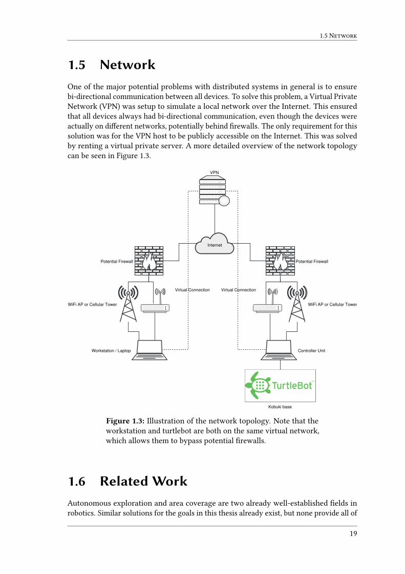
1.5 NetworkOne of the major potential problems with distributed systems in general is to ensurebi-directional communication between all devices. To solve this problem, a Virtual PrivateNetwork (VPN) was setup to simulate a local network over the Internet. This ensuredthat all devices always had bi-directional communication, even though the devices wereactually on di�erent networks, potentially behind �rewalls. The only requirement for thissolution was for the VPN host to be publicly accessible on the Internet. This was solvedby renting a virtual private server. A more detailed overview of the network topologycan be seen in Figure 1.3.

Virtual ConnectionVirtual Connection

Workstation / Laptop

VPN

Internet

Potential Firewall Potential Firewall

Kobuki base

WiFi AP or Cellular TowerWiFi AP or Cellular Tower

Controller Unit

Figure 1.3: Illustration of the network topology. Note that theworkstation and turtlebot are both on the same virtual network,which allows them to bypass potential �rewalls.

1.6 Related WorkAutonomous exploration and area coverage are two already well-established �elds inrobotics. Similar solutions for the goals in this thesis already exist, but none provide all of

19

1. Introduction

the requirements in a single platform. Below are some of the projects that can be foundonline.

Yamauchi et al. [16] developed ARIEL, a system for autonomous exploration andmap building using continuous localisation. The article describes how all the partsof the system were built up and integrated from scratch. However, the article waspublished during the late 90’s and the hardware and software used is long since obsolete.Riaz et al. [17] describe a similar system inspired by [16], but built on a more modernplatform. Unfortunately, the system is based on proprietary software, and uses algorithmsimplemented from scratch, making it hard for the community to replicate the work.

The work by Kohlbrecher et al. [18] took a di�erent approach and produced publiclyavailable open-source plug-ins based on algorithms like the Hector SLAM algorithmby Kohlbrecher et al. [19] and the exploration algorithm by Wirth and Pellenz [20].However, [18] focuses on Urban Search And Rescue (USAR) missions where modernhigh-performance LIDAR systems are available, and mentions that their performanceis high enough not to require features like explicit loop closure. This might have beentrue in their case, but will be shown in this thesis, that it is unfortunately not a universaltruth.

Some work on Wi-Fi RSS scanning in ROS has been done by Scholl et al. [21], but isin the form of a handheld unit running the algorithm mentioned above by [19]. Becauseof the algorithm used, the project could also su�er from errors that might have beencorrected by loop closures. The article seems like a start towards the same goals as inthis thesis, but no further information can be found.

This thesis acknowledges that the open-source community has implemented manyhigh-quality algorithms and does not try to re-invent the wheel. Instead it evaluates andcompares the most popular plug-ins available, to create a publicly accessible recipe foranyone to use. All of the considered plug-ins have been used as-is to the largest extentpossible, and any extensions that have been made, are publicly available on the popularsite GitHub under the organisation Robotslam1

1.7 ContributionAs seen in the previous section, there is a lot of existing material which cover theindividual components used in this thesis. This thesis instead aims to build upon theexisting knowledge to create a complete solution which can be used to solve the twouse-cases UC-Map and UC-NoMap, described in Section 1.1.2. In order to achieve this,a comprehensive evaluation of the existing material and algorithms had to be completedin order to ensure the best possible result. Furthermore, a comprehensive platform wasdeveloped to ensure that the result of the project could be used by people who possesless technical knowledge. Both authors have contributed equally to the thesis, which insummary has:

• Evaluated the performance of the most popular ROS plug-ins to make it easier forfuture projects to make a proper choice based on their requirements.

1https://github.com/robotslam

20

https://github.com/robotslam

1.8 Disposition

• Extended the popular plug-ins Gmapping and Google Cartographer with the abilityto output their trajectory over the standard ROS interface.

• Added waypoint-following capabilities to ROS by creating an entirely new globalplanner.

• Created a Wi-Fi RSS scanning plug-in which supports grouping of measurementsby time.

• Created a �eet management system to easily operate and organise data-collectionsessions by adding an abstraction layer on top of ROS.

• Extended the �eet management system with the ability to transform local co-ordinates to the latitude and longitude format used by World Geodetic System1984.

• Extended the �eet management system with the ability to correct Wi-Fi RSS meas-urement positions using trajectory data.

1.8 DispositionThe thesis is structured as mostly isolated chapters which each describe a speci�c com-ponent of the thesis project. A short summary of the chapters are provided below.

Chapter 2 Presents the methodology used in this thesis and describes the di�erentphases of the project.

Chapter 3 Provides a background to Simultaneous Localisation And Mapping, evaluatesthe di�erent SLAM algorithms, and measures the accuracy of the algorithms in aknown environment.

Chapter 4 Describes how the internal coordinates used in ROS can be converted intothe World Geodetic System 1984 (WGS84) standard.

Chapter 5 Evaluates a few existing area coverage algorithms and describes how theywere implemented.

Chapter 6 Describes frontier based exploration and evaluates the existing ROS imple-mentations.

Chapter 7 Describes how the Wi-Fi measurements were collected and how they connectto the existing infrastructure at Combain.

Chapter 8 Describes the new platform and web interface for �eet management.

Chapter 9 Ties everything together and discusses the �nal result. It also introduces acouple of topics for future work.

21

1. Introduction

22

Chapter 2

Methodology

This chapter will provide a brief overview of the methodology and the schedule of thisthesis. It also describes the di�erences between simulation and real world trials.

2.1 Approach

2 WEEKSITERATIONRESEARCH

TEST

EVALUATE

MEE

TING

IMPLEMENT

SIM

ULA

TE

WRAP-UP

Figure 2.1: Illustration of the iterative process used during thisthesis.

Due to Combain’s initial uncertainty of what was possible to achieve during a thesisproject, it was, at �rst, not possible to de�ne any formal goals. Because of this situationand the agile nature of Combain’s regular projects, it was decided to follow a moreiterative process during this thesis (see Figure 2.1).

23

2. Methodology

2.1.1 Initial ResearchTo get a better picture of what would be possible to accomplish during the length of thisthesis project (20 weeks), an initial research stage was planned for the �rst 3 weeks. Thepurpose was to gather scienti�c material and look into how much ROS was capable ofout-of-the-box. This e�ectively meant experimenting with ROS tutorials and demos, andevaluating how the existing functionality could be used in combination with publishedarticles to provide the desirable results.

In reality, this stage started to melt into the iteration process almost immediately, andthen continued as pure research in parallel to the iterations up until week 5.

2.1.2 IterationsFigure 2.1 describes the iterative process, which served as the schedule’s primary found-ation. Each iteration lasted around two weeks, and consisted of mainly �ve di�erentstages:

Meeting Each iteration started and ended with a meeting, in which the previous it-eration’s result was presented and evaluated. Afterwards the new iteration wasplanned with a new goal. This meeting was often complemented by a secondmeeting in the middle of each iteration which gave the opportunity to have morein-depth discussions.

Implement The problem statement de�ned in the meeting is researched and imple-mented. This can be anything from writing a new algorithm to tweaking existingimplementations to better �t the requirements.

Simulate The implementation is tested and veri�ed in a simulated environment. (seeSection 2.2)

Test The implementation is tested and veri�ed in a real-world environment. (see Sec-tion 2.2)

Evaluate The �nal step in each iteration is to evaluate the solution: Does it solve theproblem de�ned during the meeting and is there anything that can be improved?

2.1.3 Wrap-upThe last couple of weeks were spent wrapping everything up. This mostly consistedof writing the last parts of the report and collecting more measurements, as well ascollecting ground truth data about the environments. This data was then used to evaluatethe accuracy of the �nal solution.

2.2 Simulated and Real World TrialsAs previously described, ROS provides several tools to simulate robots and environments.In this thesis, a majority of the time was spent in a simulated environment, since it

24

2.3 Schedule

provided several bene�ts, eg. that it was much faster to prototype, since there was noneed to have physical access to the Turtlebot. Testing using a physical robot was mostlydone at the end of each iteration to con�rm real world performance.

A disadvantage with using the simulator was its di�erence to the real world. Anexample is that there does not seems to be any friction between the wheels and theground, resulting in the wheels spinning freely even when the robot is driving in to awall.

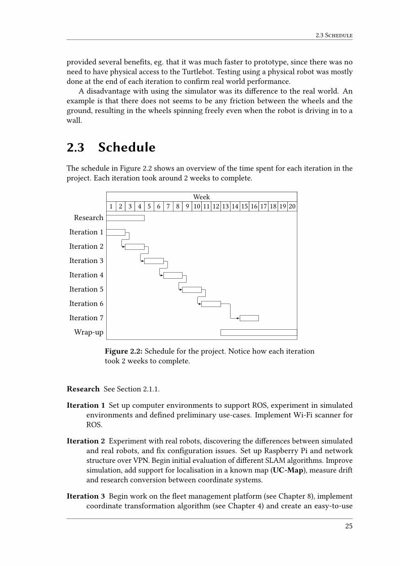
2.3 ScheduleThe schedule in Figure 2.2 shows an overview of the time spent for each iteration in theproject. Each iteration took around 2 weeks to complete.

Week1 2 3 4 5 6 7 8 9 10 11 12 13 14 15 16 17 18 19 20

Research

Iteration 1

Iteration 2

Iteration 3

Iteration 4

Iteration 5

Iteration 6

Iteration 7

Wrap-up

Figure 2.2: Schedule for the project. Notice how each iterationtook 2 weeks to complete.

Research See Section 2.1.1.

Iteration 1 Set up computer environments to support ROS, experiment in simulatedenvironments and de�ned preliminary use-cases. Implement Wi-Fi scanner forROS.

Iteration 2 Experiment with real robots, discovering the di�erences between simulatedand real robots, and �x con�guration issues. Set up Raspberry Pi and networkstructure over VPN. Begin initial evaluation of di�erent SLAM algorithms. Improvesimulation, add support for localisation in a known map (UC-Map), measure driftand research conversion between coordinate systems.

Iteration 3 Begin work on the �eet management platform (see Chapter 8), implementcoordinate transformation algorithm (see Chapter 4) and create an easy-to-use

25

2. Methodology

interface for it. Save Wi-Fi measurements to �le and convert to GPS coordinates.Implement global planner for following waypoints and switch over to using anotebook instead of a Raspberry Pi.

Iteration 4 Research exploration, and path coverage. Implement and evaluate path cov-erage based on the path transform algorithm (see Chapter 5). Path coverage worksautonomously for the �rst time. Initial evaluation of most popular explorationalgorithm.

Iteration 5 Experiment with 3D depth camera and major improvements to the �eetmanagement platform’s functionality and usability. Exploration works autonom-ously for the �rst time and the collected measurements are successfully exportedto Combain’s system.

Iteration 6 Automation of export to Combain’s system and other general improvementsto �eet management platform. Test cli� sensors. Further test exploration andimprove positioning of measurement after loop closure using trajectories.

Iteration 7 Further investigation in area coverage, implemented spanning tree coverageand evaluated it against distance path transform.

Wrap-up Collect reference (ground truth) data, perform more measurements and evalu-ate the results. Finish report. See Section 2.1.3.

26

Chapter 3

Simultaneous Localization AndMapping

Simultaneous Localisation And Mapping is a well-researched topic in many areas, in-cluding mobile robotics. ROS provides several ready to use implementations of di�erentSLAM algorithms. In this chapter the most popular algorithms, Gmapping, Cartographer,and Hector SLAM are presented and evaluated to see which one provides the best resultfor UC-NoMap. The focus will not be on researching or implementing new algorithmsrelated to SLAM.

3.1 MotivationHaving an accurate SLAM algorithm can be motivated in many ways. While the goal ofthis thesis is not to create high-resolution indoor maps, they play a vital role as they areused to place the measurements in the real world. In order to achieve this, there is a needfor an accurate description of how the robot has travelled, i.e. the trajectory.

3.2 OpenSlam’s GmappingGmapping is the default provided SLAM algorithm in ROS. It uses LIDAR and odometrymeasurements to locate and map its surroundings. It is based on Rao-BlackwellizedParticle Filters and supports loop closure. The articles [22, 23] describe the actual al-gorithm in detail. The standard con�guration of Gmapping also relies heavily on anexternally provided odometry. This means that inaccurate sensor readings will be detri-mental to the mapping result.

27

3. Simultaneous Localization And Mapping

3.2.1 ImpressionThe �rst hands-on experience in the simulated world was promising, resulting in mapsthat mostly managed to correct themselves when the robot arrived back at known territory.A small issue was how the algorithm reacted when driving into a wall, where the wholemap would drift at the same speed as the robot’s simulated wheels, as if the map wasmoving away from the robot. The problem seemed to originate from the simulatorreporting positive wheel speed even though the robot was not actually moving. Thebehaviour could not be replicated in the real world since the bump sensor would triggerand reverse the robot away from the wall.

When Gmapping was �rst used in the real world, the algorithm su�ered from anissue that made the map “hairy” as seen in Figure 3.1a. After closer inspection, it wasconcluded that the hairs were missing LIDAR points which the algorithm interpretedas free space with the same radius as the LIDAR’s speci�ed maximum range. The hairswere successfully removed by con�guring Gmapping to ignore LIDAR values past itsmaximum rated range. The algorithm then performed as good as it did in the simulatedworld.

3.2.2 Loop ClosureGmapping does not have a dedicated method for identifying loop closures, instead it isa consequence of how the algorithm itself works. In short, Gmapping always keeps aprede�ned number of randomly generated particles, i.e. hypotheses of how the robot hastravelled. Combined with what the robot has seen at every scan a map can be drawn forevery particle. Because these particles also have a continuously re-evaluated likelihoodattached, the most likely particle is the one used to draw the map which is displayed tothe user. The likelihood is calculated by comparing the last LIDAR scan with what thedi�erent particles predict. In long featureless corridors, it is therefore hard to determine ifthe particle which has travelled e.g. a few centimetres further than another is the correctone or not, because both predict equal scans. However, when the robot �nally arrivesback to a known feature-full territory, the algorithm quickly identi�es the most likelyparticle and the map changes.

3.3 Hector SLAMHector SLAM is based on the paper by Kohlbrecher et al. [19] which does not requireany other data than LIDAR measurements. It has support for IMU sensors to compensatefor tilt but no loop closure.

The Hector SLAM algorithm is described in [19] as consuming “low computationalresources” and mention that other algorithms do not “leverage the high update rateprovided by modern LIDAR systems”. The mentioned LIDAR system is most likely areference to the Hokuyo UTM-30LX LIDAR device used in [19], which has a scan frequencyof 40 Hz (compared to the 5 Hz of the LIDAR device used in this project).

28

3.3 Hector SLAM

(a) Gmapping result.

(b) Hector result.

(c) Google cartographer result.

Figure 3.1: Mapping exjobbsrummet (room reserved for studentsdoing their master’s thesis) in the M-building on the LTH campus.

29


3.3.1 ImpressionHands-on experience in the simulated world showed great promise with little to no drift,i.e. the robot was always where the algorithm said it was. The results strengthened theclaim made by Kohlbrecher et al. [19] that in many scenarios, optimisations such as loopclosure are not needed. Furthermore, since the algorithm does not utilise the odometry,it did not su�er from the same problems as Gmapping in which the simulator reportedmovement on the wheels while the robot stayed still.

However, the real world testing was a disappointing exercise. While straight move-ments were tracked accurately, rotation was a complete disaster. The cause might havebeen the low scan rate of the LIDAR device. Because of this, the idea of using HectorSLAM was abandoned early in the project. An example of a map created by Hector canbe seen in Figure 3.1b.

3.4 Google CartographerCartographer is a real-time SLAM library developed by Google and was recently open-sourced in October 2016. It supports loop closure and IMU sensors to compensate for tiltand also enable 3D tracking. It is based on the paper by Hess et al. [24]. More informationon how it di�ers from the other algorithms can be seen below.

3.4.1 ImpressionCartographer was unique in o�ering the same impression in both the simulated environ-ment and the real world. Cartographer was also unique in being able to produce mapswhich contained information on the likelihood of an area being occupied or free. Thiswas done by allowing the map to hold the entire range of values between black and white,representing the likelihood that a certain space contains an obstacle. In comparison,the other two algorithms only use the three discrete values: white, grey and black torepresent: free, unknown and occupied space.

3.4.2 Loop ClosureCartographer contains a more explicit loop closing method which is separate from itsmain algorithm, this makes it di�erent to Gmapping. In short, Cartographer continuouslycreates small localised maps from very few LIDAR scans, called submaps. These submapsare stored as nodes in a graph structure, where geographical constraints are addedbetween the nodes as edges. This graph is then treated as a large optimisation problemand solved using the Ceres solver, and the solution is then used to draw the map. Loopclosure is accomplished, in a separate process, by identifying relationships betweennearby, but previously unrelated nodes in the graph using scan matching. By adding anedge between these nodes, the next time the map is drawn the nodes will be linked andthe loop closed.

30

3.5 Evaluation

3.5 EvaluationA critical requirement in this thesis is to ensure the accuracy of the produced trajectory.This can be done by ensuring an accurate map, since the map serves as the foundationfor the trajectory, which in turn is used to map the measurements to real world positions.

The tests were conducted by manually controlling the robot using the provided ROSpackage teleop, which allows for remote operation using a keyboard. All the sensordata was recorded using the ROS package rosbag, which allows the recorded data to bere-played at a later time. This way it was possible to run the exact same scenario multipletimes using di�erent SLAM algorithms.

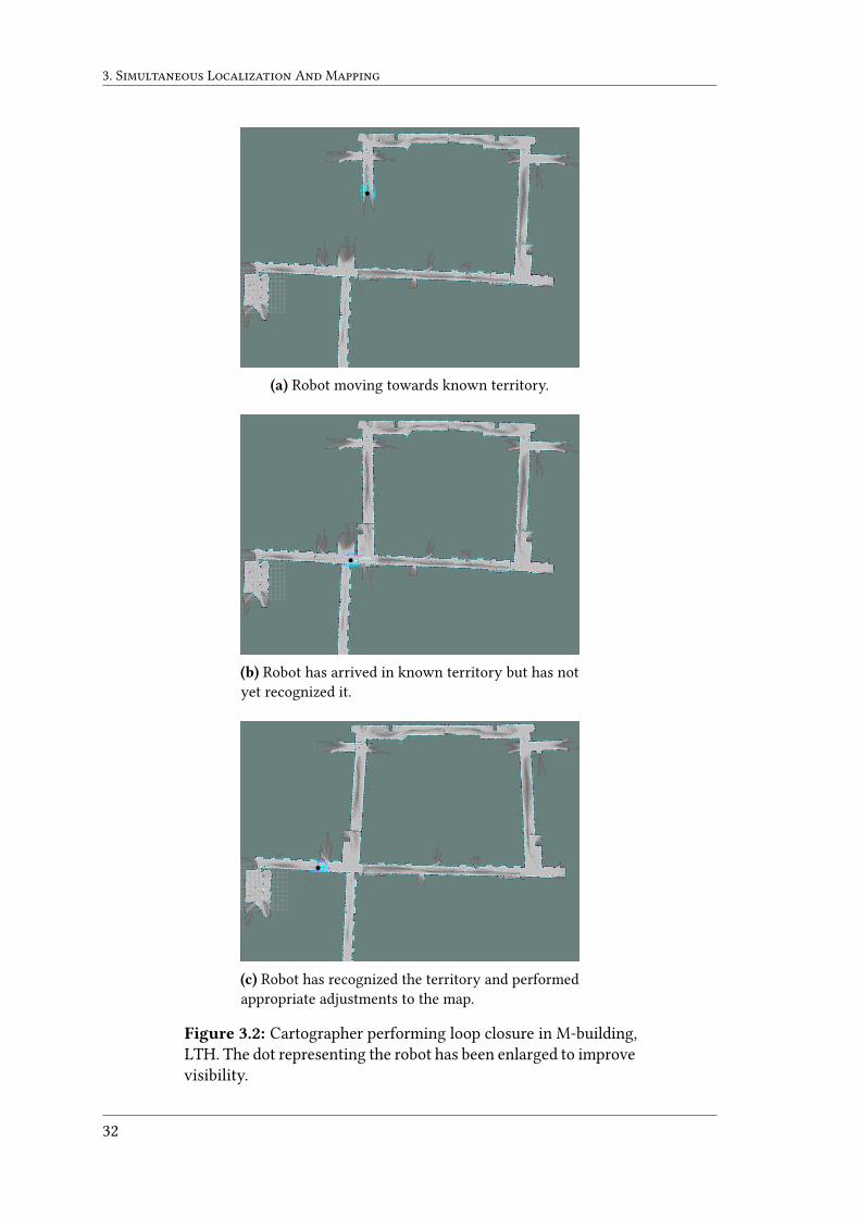
3.5.1 Loop ClosureLoop closure is a critical part of mapping which continuously tries to match the currentlocation with previously visited ones. It mitigates erroneous overlapping by matchingnew scans with old ones and adjusting the map, and current position, accordingly. Asmentioned above, both Gmapping and Cartographer support some form of loop closure.An example of Cartographer performing loop closure can be seen in Figure 3.2. However,since loop closure does not refer to a single method, the evaluated algorithms each havetheir own techniques.

In practice, these techniques produced very di�erent results. For example, in Figure 3.3it can easily be seen how the randomisation part of Gmapping produces unique resultsevery time the algorithm is executed on the same data set. This unfortunately means thatGmapping has the same negative intrinsic property that all particle �lters have — theinability to deterministically guarantee a good solution.

Cartographer, on the other hand, has succeeded in closing the loops every single time,as can be seen in Figure 3.3. Combined with the fact that Cartographer is based on adeterministic algorithm, it clearly stands out from the rest.

In summary, by failing to close loops 77% of the time, Gmapping performs signi�cantlyworse than Cartographer, something which can happen in even the best of circumstancesdue to the uncertain nature of the algorithm. When the loops are closed however, theyseem to get a lot less distorted by Gmapping than Cartographer, as can be seen inFigure 3.4.

3.5.2 AccuracyTo determine the accuracy of the maps, the physical location was measured using alaser range�nder. The range�nder had a maximum range of 50 m with an accuracy of±2.0 mm. However, because the range�nder was operated by hand, the �nal result couldrealistically only have had decimetre accuracy.

Since Gmapping uses a non-deterministic algorithm, it was decided to replay the data10 times and calculate the mean distances in order to get a more accurate comparison.The test results which can be seen in Table 3.1 shows that the mean error for Gmappingwas 1.9%, Cartographer on the other hand had a higher mean error of 2.3%, but since ithad a deterministic behaviour it tended to provide more reliable results.

31


(a) Robot moving towards known territory.

(b) Robot has arrived in known territory but has notyet recognized it.

(c) Robot has recognized the territory and performedappropriate adjustments to the map.

Figure 3.2: Cartographer performing loop closure in M-building,LTH. The dot representing the robot has been enlarged to improvevisibility.

32

3.5 Evaluation

Loop closing success rate: 10%

0

1

2

3

4

5

6

7

8

9

10

(a) Gmapping 2017-03-31-01


0

1

2

3

4

5

6

7

8

9

10

(b) Cartographer 2017-03-31-01


0

1

2

3

4

5

6

7

8

9

10

(c) Gmapping 2017-04-06-01


0

1

2

3

4

5

6

7

8

9

10

(d) Cartographer 2017-04-06-01


0

1

2

3

4

5

6

7

8

9

10

(e) Gmapping 2017-04-06-02


0

1

2

3

4

5

6

7

8

9

10

(f) Cartographer 2017-04-06-02

Figure 3.3: Visualisation of the di�erent outputs from mul-tiple runs of the same algorithm on the same data sets. Noticehow Gmapping produces di�erent maps every time while Carto-grapher does not. Notice also how Gmapping fails to close theloop and how Cartographer succeeds, but distorts the map in theprocess.

33


(a) Gmapping. (b) Cartographer.

Figure 3.4: A comparison between Gmapping and Cartographerwhen both have successfully closed a loop. Notice how Carto-grapher distorts the map compared to Gmapping.

Another critical criteria which Gmapping had large issues with was loop closure, asmentioned in Section 3.5.1. The length of the corridors were still accurate, but because ofthe failed loop closures, the last corridor failed to line up correctly.

Both algorithms had problems handling the left corridor where the error rangedbetween 0.3 m − 1.8 m. In comparison, the bottom corridor only had a maximum errorof 0.3 m, lending to the conclusion that some corridors are easier to map than others.

Table 3.1: Measurements in M-huset at LTH. Note that for Gmap-ping, the error of each corridor was calculated as an average over10 algorithm executions for each data set.

Left Top Right Bottom ErrorReference 32.1 41.3 32.2 44.7Gmapping #1 31.7 40.7 32.0 43.3 2.6 (1.7%)Gmapping #2 31.1 40.7 31.5 44.3 2.7 (1.8%)Gmapping #3 31.8 40.2 31.5 43.4 3.4 (2.3%)Cartographer #1 31.5 39.8 31.6 44.4 3.0 (2.0%)Cartographer #2 30.3 40.9 32.0 44.3 2.8 (1.9%)Cartographer #3 30.4 39.2 31.9 44.4 4.4 (2.9%)

3.5.3 PerformanceOne of the original criteria for the project was the ability to use a Raspberry Pi as thecontrol unit for the robot. This put a lot of requirements on the algorithms since it limitedthe available data transfer bandwidth. For the SLAM algorithms to be able to run andproduce usable results, the settings, primarily the resolution of the algorithms, had tobe tweaked. This in turn resulted in a less than satisfying result, and ultimately leadto replacing the Raspberry Pi with a more powerful notebook. All of the results in thisreport have been produced on the notebook.

Figure 3.5 shows a performance benchmark of the evaluated SLAM algorithms. Itshows how Cartographer uses much less resources on smaller maps, but eventually moves

34

3.5 Evaluation

0 100 200 300 400 500 600 7000

10

20

30

40

50

60

70

80

90

100

Seconds

%CP

U

Gmapping (0.05m) Cartographer (0.05m)Gmapping (0.1m) Hector (0.05m)

Figure 3.5: Performance comparison of the di�erent algorithmsrunning data set 2017-04-06-02, executed on the notebook. Notethat Linux measurements treat each logical core as a separateCentral Processing Unit (CPU), meaning that on a quad-core CPU,the maximum percentage is actually 400%. The above algorithmstherefore either heavily utilise a single core, or lightly utilisemany cores.

up as the map gets bigger. An interesting part is how, at the same time, Gmapping seemsto have a downward trend, using up less resources as time goes on. The reason for thisbehaviour has not been uncovered, but a hypothesis is that Gmapping might begin tomiss or throw away incoming data. This might happen because Gmapping does notbu�er the input, which e.g. leads to unusable maps when speeding up the replay of therecorded data-sets. Either that or the measurement method was, in some way, inaccurate.

Either way, Gmapping had an average of 82% and 75% CPU usage for 0.05 m and0.1 m resolutions, while Cartographer had an average of 44%. This means Cartographeris the clear winner over Gmapping in utilising the CPU e�ciently.

3.5.4 TrajectoryThe trajectory describes the path which the robot has travelled. In order to ensure thatthe collected measurements can accurately be mapped to speci�c locations, it is important

35


to ensure that the trajectory is accurate.Simply storing the current position of the robot when a measurement is taken is not

su�cient, since the trajectory can and will change during a loop closure. Therefore, animportant criteria when selecting an algorithm, is to ensure the accuracy of the �naltrajectory. Figure 3.6 shows the di�erence between collecting the current position duringeach measurement and using the trajectory.

Sadly, neither Gmapping or Cartographer exposed the trajectory using the standardROS interface. However, after some investigation it was discovered that both algorithmskept an internal representation of the trajectory. Both algorithms were therefore modi�edto enable access to the trajectory over the ROS interface.

Since Hector SLAM does not support loop closure, previous locations in the trajectoryare never modi�ed. In this case, it is therefore su�cient to simply save the currentlocation when a measurement is taken.

3.5.5 ConclusionThe purpose of this chapter has been to present and evaluate which of the most popularROS plugins for SLAM provide the best results for UC-NoMap. After gathering a widerange of statistics, the algorithm that has stood out the most has been Cartographer.However, while Hector SLAM has been a clear loser, the distinction between Gmappingand Cartographer has not been clear. Gmapping provides less warped maps and canuse odometry data in a way that Cartographer can not. On the other hand, the warpingonly increases the mean error by 0.4 p.p. and judging by how good Hector performsin the original article [19], odometry is not a problem when a high-performing LIDARis used. Therefore, after the risk of Gmapping failing at loop closure was factored in,Cartographer was chosen as the recommended algorithm.

36

3.5 Evaluation

Continuous sampling Trajectory

Figure 3.6: Comparison between continuously sampling andstoring the position, and the �nal trajectory. Notice how thecontinuous sampling in the top corridor contains sudden jumpswhere Gmapping has switched between particles. The trajectorylooks like a smoother and more accurate representation of howthe robot might have moved. Notice also that Gmapping hasfailed to close the loop, and that the left-most parallel corridorsare in reality the same corridor.

37


38

Chapter 4

Local CartesianCoordinates toWGS84

ROS uses a local cartesian coordinate system to represent the position of the robot. Inorder for these coordinates to be usable by external systems, such as Combain PositioningService (CPS), they need to be converted into a global reference coordinate system. SinceCPS already supports the WGS84 standard for use when submitting reference points, itwas the natural choice. This chapter presents how an a�ne transformation can be usedto make this conversion with su�cient accuracy.

4.1 TransformationA method of transforming points from one coordinate system to another is to use an a�netransformation matrix. This method uses three reference points to create a transformationmatrix between the two systems. The method is well known and well documented, but aquick summary can be read below.

If uwgs ∈ R2×3 are the coordinates of three points in WGS84 and ulocal ∈ R2×3 are thesame points in the local coordinates the relationship between the two can be de�ned as

uwgs = A · ulocal + t, (4.1)

where A is the transformation matrix and t is an o�set vector. Using an augmentedmatrix and an augmented vector, it is possible to represent both the translation and theo�set using a single matrix multiplication,[

uwgs1

]=

[A t0 1

] [ulocal

1

]⇔ vwgs = T · vlocal. (4.2)

In detail this is the same asxwgs1 xwgs2 xwgs3

ywgs1 ywgs2 ywgs3

1 1 1

=a c txb d ty0 0 1

xlocal1 xlocal2 xlocal3ylocal1 ylocal2 ylocal3

1 1 1

. (4.3)

39

4. Local Cartesian Coordinates to WGS84

Assuming that the reference points have been properly chosen i.e. not linearly dependent,the transformation is easily retrieved by multiplying with the inverse of vlocal from theright on both sides:

T = vwgs · v−1local. (4.4)

The transformation matrix is now able to transform any points in any direction betweenthe two coordinate systems.

4.2 Error EstimationBecause WGS84 coordinates are not linearly distributed, using a (linear) transformationmatrix results in an approximation error. A quick estimation of this error was done bycalculating the di�erence in length between a sphere (earth approximation) and a tangentplane (transformation plane built up by the transformation matrix).

l

rθ

d

Figure 4.1: Cross section of an earth approximated as a sphereand a tangential transformation plane.

To calculate the error in any given direction, the distances d and l from the point oftangency between the sphere and its tangent plane (see Figure 4.1) need to be identi�ed.By setting up the distance equations

tan(θ) =lr⇔ l = r · tan(θ) (4.5)

andd = r · θ, (4.6)

the error can be de�ned as the di�erence between the two distances

ε = l − d = r tan(θ) − rθ = r(tan(θ) − θ). (4.7)

After setting r = 63710088 to the mean radius R1 of earth [25] the error is plotted as afunction of the distance d (see Figure 4.2). The plot shows that even a kilometre awayfrom the point of tangency, the error is still below 0.1 µm. This leads to the conclusion

40

4.2 Error Estimation

0 200 400 600 800 1,0000

1

2

3

4

5

6

7

8

9·10−8

Distance from point of tangency (metres)

App

roxi

mat

ion

erro

r(m

etre

s)

Figure 4.2: A�ne transformation error plotted up to 1 km.

that using an a�ne transformation matrix yields far to small an error for it to have anymeaningful a�ect on the transformation of measurements made inside a single building.

It is worth noting that two major assumptions have been made in this estimation.The �rst is that the transformation plane is a tangent plane while in reality it is actuallya plane that cuts the sphere. This is because the three reference points do not coincide.However, compared to the radius of the earth, the distance between the reference pointsis so small that the points are assumed to converge. The second assumption is that theearth is a perfect sphere with the radius 63 710 088 m. This radius is actually the meanradius of the earth which means that the error estimation above is actually an estimationof the average case. However, this fact is assumed to have a negligible impact on shortdistances.

41

4. Local Cartesian Coordinates to WGS84

42

Chapter 5

Area Coverage

Area Coverage is another well-researched topic in mobile robotics, which fairly recentlyhas made its way into households in the shape of robot vacuum cleaners and lawnmowers.In this chapter two existing algorithms: spanning tree covering, and distance transformpath, are evaluated to see which can best be applied to this thesis.

5.1 MotivationArea Coverage can be seen as a generalisation of the well known Travelling SalesmanProblem (TSP) and is therefore NP-Hard, i.e. solving the optimisation cannot (currently)be done in polynomial time [26]. Therefore, an algorithm which �nds an approximatesolution is necessary. The criteria for selecting an algorithm are: it should �nish in a �nitetime, cover as much of the area as possible, and return a path which can be completed asfast as possible.

The robots characteristics have to be taken into consideration since less distancetravelled does not necessarily mean that the time required to complete the path is less.The Turtlebot 2 tends to handle tight curves badly by slowing down drastically. Therefore,a solution which requires as few tight curves as possible would be preferable. The areacoverage part of this thesis is used to solve the UC-Map.

5.2 Adaptive Monte Carlo LocalisationChapter 3 covered how it is possible to create a map using SLAM algorithms in unknownenvironments. But in the event that the environment has already been mapped, andthe map exists (UC-Map), it is preferable to use the existing map rather than creatinga new one. The advantages are: better planning possibilities and better completion-time estimates. This is where Adaptive Monte Carlo Localisation (AMCL), a localisation

43

5. Area Coverage

algorithm, comes in. AMCL shares some similarities with Gmapping in that they areboth based on particle �lters. However, instead of collecting sensor data and building amap, AMCL uses an existing map and identi�es the robots position relative to it.

5.3 Global Planner

The coverage algorithms below, all produce a path as an output, but because the navigationstack in ROS is built to only accept a single goal as input (see Section 1.2.1), a customsolution was needed in order to combine the two.

A global planner called remote_global_planner was implemented. The planner acceptsa pre-generated path, and ignores the goal input usually sent to the navigation stack.The path consists of a series of way-points, which get forwarded to the local planner forexecution. This approach, as opposed to implementing the coverage algorithms straightinto the planner, was chosen because of Combain’s requirement to o�oad as much ofthe processing as possible (see Section 1.1.1). Having the planner accept remote plansopens up the possibility of calculating these paths on a remote server or even in advance.

One problem that was discovered was the fact that the local planner is fairly bad atfollowing way-points, and prefers to ignore them if it can reach the goal faster by doingso. To avoid this issue, the remote_global_planner only sends a few way-points at a time,leaving the local planner without a path to skip to. The disadvantage with this method isthat the robot might slow down or even stop moving for short moments while the localplanner calculates a new path to the next way-points.

To allow the robot to adapt to dynamic changes in the world, the remote globalplanner uses one of the existing single-goal algorithms provided by ROS , to plan thepath to the next way-point. Obstacles such as people walking by or other things notpresent when the map was generated is therefore avoided by the robot.

5.4 Execution Time Estimation

To be able to compare the algorithms below, a formula for modelling the execution timeof a path was needed. By measuring how much time a path takes to execute if it containsturns, and then measure the same path without turns, the average impact that each turnhas can be calculated. While performing these measurements it was found that < 180°turns actually improve the execution time, i.e. it takes less time to complete a path withthese turns. This is a consequence of how the local planner tends to take shortcuts, aspreviously mentioned in Section 5.3. The resulting formula, valid for cell sizes around

44

5.5 Occupancy Grid

0.5 m, is:

Time = L0.5− 0.36T45 − 0.14T90 − 2.8T180 + 5.3Tmax,

where Time = predicted execution time in seconds,T45 = amount of turns where angle ≤ 45°,T90 = amount of turns where 45° < angle ≤ 90°,

T180 = amount of turns where 90° < angle < 180°,Tmax = amount of turns where angle = 180°.

5.5 Occupancy GridAn occupancy grid is a way to represent a map as a discrete grid. Internally, ROS usesa probability occupancy grid, i.e. each cell has a value between 0–100 to represent theprobability of the cell being occupied. However, not all ROS plug-ins take advantage ofthe entire range, and instead divide it into three parts: free, unknown and occupied. Themap_server plug-in, which is used to save a map to disk, exhibits this exact behaviour.Some �gures in this thesis will therefore have three colours, while some will have theentire range from black to white.

Since an occupancy grid stores the world in a grid map of a speci�c resolution, itsu�ers from the traditional issues of approximate representations. Namely lack of detailsbelow the speci�ed resolution, which makes it impossible to deduct if whole cells areoccupied or just some parts of them.

5.5.1 DownscalingThe occupancy grid is an approximate representation of reality using cells with sizesequal to the resolution. Because both algorithms presented below use occupancy gridsas input, it would be possible to use the maps produced during the SLAM sessions (seeChapter 3) directly. However, these maps have a resolution of around 0.05 m – 0.1 mwhich, without any pre-processing, would result in a coverage of the same magnitude asthe resolution, i.e. the robot would drive over every 0.05 m.

To be able to choose how detailed the area coverage should be, the occupancy grid is�rst down-scaled before used as input for the coverage algorithms. This is accomplishedby using a method called box sampling. Simply put, if a coverage of d metres is desired,the process looks as follows:

1. Overlay the original occupancy grid O with another grid G of size d.

2. For each cell in G, calculate the average values of the corresponding cells in O.

3. Assign the average value to each cell in G and treat G as a new occupancy grid.

To further simplify the process, each cell in G is treated as occupied if its value is largerthan vthresh, and unoccupied otherwise. To guarantee a viable solution, vthresh is set tov f ree+1, meaning that even a single occupied cell in O results in the entire cell in G being

45

5. Area Coverage

Figure 5.1: To the left is a visualisation of a graph representationof a 10 m×10 m map. On the right is a visualisation of a spanningtree of the same graph.

marked as occupied. By using G as an input to the algorithms below, complete coverageof every, completely empty, d metre is guaranteed.

5.6 Spanning Tree Covering

The paper by Gabriely and Rimon [26] describes a novel method of using a spanningtree for area coverage. This can be accomplished by interpreting all of the free cells inthe occupancy grid as vertices in a graph. By adding edges between all vertices thatrepresent adjacent cells in the occupancy grid, a graph like the one in Figure 5.1 can beobtained. A spanning tree, which is de�ned as a sub-graph that is a tree and contains allthe vertices with the minimum number of edges, can then be constructed by using e.g.Prim’s algorithm [27]. An example of a spanning tree can also be seen in Figure 5.1.

After a spanning tree has been constructed, coverage can be obtained by: dividing allcells into four sub-cells, selecting any cell as the initial starting position and then walkingalong the tree until the initial cell is encountered again. In other words, imagine placingyour left hand anywhere on the tree and simply walking straight, making sure to neverstop touching the tree. Eventually you will have circumnavigated the entire tree in acounterclockwise direction and end up where you started. This also means that you willhave covered the entire map. An example can be seen in Figure 5.2, which is the pathgenerated by the spanning tree in Figure 5.1.

The paper [26] actually presents three di�erent algorithms. However in this thesis,only the o�ine variant called O�ine STC was considered, as it is the only one whichuses known maps.

46

5.7 Distance Transform Path Planning

Figure 5.2: Generated path from the spanning tree in Figure 5.1,notice how the path circumnavigates the spanning tree.

5.7 Distance Transform Path PlanningThe paper by Zelinsky et al. [28] presents “a solution to the problem of complete coveragebased upon an extension to the distance transform path planning methodology”. Thealgorithm is explained in further detail below.

5.7.1 Distance TransformThe distance transform Tdist is a matrix where every element describes the distance to aspeci�c element vgoal. In this thesis, Tdist is calculated using the Breath First Search (BFS)algorithm. An illustration of a distance transform calculated using BFS can be seen inFigure 5.3. The coverage path is then created by moving along the path of steepest ascent.This means that the path moves away from the goal while keeping track of the cells ithas already visited.

[28] mentions that “the robot only moves into a grid cell which is closer to the goal ifit has visited all the neighbouring cells which lie further away from the goal”. This thesisuses an alternative approach by introducing a backtracking method. The backtracking isactivated when the robot ends up at a dead-end, formed either by obstacles or cells whichhave already been visited. To perform the backtracking, the algorithm simply walksbackwards along the path until it reaches a neighbour which has not been visited. Thisneighbour is then added immediately after the dead-end cell, ignoring the backwardswalk. This technically means that the path usually ends up across obstacles, but this isnot a problem since the global planner will automatically adapt using the single-goal

47

5. Area Coverage

algorithm.

5.7.2 Path TransformThe paper [28] also describes a transform for planning called path transform Tpath. Itbuilds upon the distance transform Tdist by combining it with a transform called obstacletransform Tobst . The obstacle transform can be described as a matrix where every elementdescribes the minimum distance to the closest obstacle. Every element c in Tpath is thencalculated using the function:

PT (c) = minp∈P

length(p) +∑ci∈p

αobstacle(ci)

. (5.1)

According to the results in [28] Tpath results in paths which tend to follow walls, resultingin overall straighter paths.

In this thesis, the path transform was implemented by modifying the distance trans-form algorithm to use Dijkstra’s algorithm with PT (c) as input. However, while themodi�cation did add complexity to the algorithm, the results did not improve nearly asmuch. In fact, while in small maps like in Figure 5.3 the path had a tendency to followwalls, there was no improvement at all in bigger ones like in Figure 5.5. The reason whyis not clear, maybe the map was simply too uneven, or maybe the implementation waserroneous in some way. Because of this, the path transform was not used in the �nalevaluation of this chapter.

5.8 EvaluationThe results from both algorithms are presented in Table 5.1, from which it is possible tosee that spanning tree covering resulted in a drastically shorter distance travelled, witha more than 15% improvement for the small 20x20 example and a 60% improvementfor M-huset. However since the distance transform path actually covered a larger areain M-huset this is not a completely fair comparison. One of the reasons the distancetransform path algorithm performed badly was due to the need to backtrace whenever itgot stuck, which might have been improved with a more e�cient method such as �ndingthe closest uncovered area and continuing.

Looking at the output of the spanning tree covering algorithm it is clearly visible thatit resulted in a sub-optimal path due to a high number of necessary turns in the top andbottom corridors which was caused by the map being at a slight rotation. After rotatingthe map by 13° the amount of turns was decreased for both algorithms. The result wasparticularly noticeable on STC since it resulted in a 34 % decrease of the number of turns.

To verify the accuracy of the execution time model, a smaller area of M-huset wastested. The di�erence between the planned and the actual travelled path, together withthe corner cutting, can be seen in Figure 5.6. The model predicted an execution time of9 min 53 s for the distance transform path and 6 min 25 s for the spanning tree coveringpath. The actual execution times were 8 min and 5 min 25 s respectively, meaning thatthe prediction was o� by a bit more than 20 % for both paths.

48

5.8 Evaluation

S 19 13 13 13 13 13 13 13 13 13 13 13 13

18 18 12 12 12 12 12 12 12 12 12 12 12 12

17 17 11 11 11 11 11 11 11 11 11 11 11 11

16 16 11 10 10 10 10 10 10 10 10 10 10 10

15 15 11 10 9 9 9 9 9 9 9 9 9 9

15 14 11 10 9 8 8 8 8 8 8 8 8 8

15 14 13 12 11 10 9 8 7 7 7 7 7 7 7 7

15 14 13 12 11 10 9 8 7 6 6 6 6 6 6 6

15 14 13 12 11 10 9 8 7 6 5 5 5 5 5 5

15 14 13 12 11 10 9 8 7 6 5 4 4 4 4 4

15 14 13 12 11 10 9 8 7 6 3 3 3 3

15 14 13 12 11 10 9 8 7 7 3 2 2 2

15 14 13 12 11 10 9 8 8 8 3 2 1 1

15 14 13 12 11 10 9 9 9 9 3 2 1 G

15 14 13 12 11 10 10 10 10 10 3 2 1 1

15 14 13 12 11 11 11 11 11 11 3 2 2 2

Figure 5.3: Illustration of a distance transform matrix, blacksquares represent obstacles, and the numbers are the distances tothe goal. Notice, that diagonal neighbours are allowed.

49

5. Area Coverage

Figure 5.4: Illustration of the Planned Path from DT in Figure 5.3.The start position is in the top left corner. The path always pickthe neighbouring node with highest cost.

Even though the prediction was o� by 20 %, the model still seemed to provide anaccurate di�erence between the two algorithms. However, using the formula to predictthe execution times for the paths in Table 5.1 was an entirely di�erent story. While thepaths generated by the spanning tree algorithm for M-huset were believably predicted at55 min, the prediction for the distance transform path turned out to be negative (−90 min).Because of this, the prediction model could unfortunately not be used for any type ofcomparison between these algorithms. The paths generated by the distance transformalgorithm were simply to complex.

5.9 ConclusionIn this chapter the purpose has been to present and evaluate some popular algorithmsfor area coverage to see which provide the best results for UC-Map. As was mentionedin the beginning of this chapter, two criteria had been chosen for the evaluation of thesealgorithms. The primary was complete map coverage and the secondary was executiontime.

As can be seen in Figure 5.6, both algorithms covered the majority of the area. How-ever, it is quite clear that the distance transform algorithm provided a better coverage thanthe spanning tree algorithm. Regarding the second criteria, the spanning tree algorithmprovided both better execution times during testing, and shorter paths. The conclusionin this chapter is therefore that the recommendation depends heavily on the speci�cuse-case. Even so, the authors would like to recommend the spanning tree algorithm,as it is felt that the di�erence in path length is worth sacri�cing some coverage over.

50

5.9 Conclusion

(a) Distance transform path

(b) Spanning tree covering

Figure 5.5: Visualisation of the full path in M-huset

51

5. Area Coverage

Table 5.1: Statistics for the two area covering algorithms fordi�erent maps, using a 0.35 m cell size.

Map Alg. Coverage Dist. Number of turns[m] Total < 45° 90° 180°

20 × 20 STC 232 / 232 231 48 0 0 0 48 0 0DTP 232 / 232 272 144 0 57 0 29 61 1

M-huset STC 10376 / 10384 1816 2317 0 0 0 2317 0 0DTP 12457 / 12457 2738 8556 48 3691 16 1233 3487 81

RotatedM-huset

STC 10560 / 10568 1848 1525 0 0 0 1525 0 0DTP 12487 / 12487 2703 7491 40 3168 17 1022 3208 36

Planned path Travelled path

(a) Distance transform path

Planned path Travelled path

(b) Spanning tree covering

Figure 5.6: Comparision betweeen the planned and actually trav-elled paths of the bottom left cooridor in M-huset.

However, it should be noted that the spanning tree algorithm, in the worst case scenario,would only provide a 50 % coverage.

52

Chapter 6

Exploration

This chapter covers autonomous exploration of an unknown map. A few of the existingalgorithms are presented and evaluated to recommend the one which provides the bestresult for UC-NoMap.

6.1 MotivationThe exploration algorithm’s main purpose is to provide the autonomy part ofUC-NoMap.The algorithm takes a time consuming process and automates it by letting the robotexplore the layout of a building by itself.

6.2 Frontier-based ExplorationThe paper by Yamauchi [29] describes a novel method of using a frontier-based approachfor exploration. According to the paper, “To gain the most new information about theworld, move to the boundary between open space and uncharted territory”. A frontieris hence de�ned as the edge between open space and the unknown. The paper doesmention that “A Zeno-like Paradox where the new information contributed by each newfrontier decreases geometrically is theoretically possible (though highly unlikely)”, butalso says that even in such cases “the map will become arbitrary accurate in a �niteamount of time.”

6.3 Selection of FrontierOne of the ways to improve the performance of the exploration is to ensure the selec-tion of good frontiers. The paper by Holz et al. [30] evaluates di�erent strategies for

53

6. Exploration

selecting frontiers. It shows that selecting the closest frontier, results in a fairly optimalsolution, though a slight improvement is possible by using repetitive re-checking1 andmap segmentation2.

6.4 Existing ImplementationsThere currently exist multiple implementations of the frontier exploration for ROS. Forthis thesis it was decided to evaluate three di�erent implementations to see if there existsa di�erence in the performance.

6.4.1 Frontier ExplorationThe paper by Yamauchi [29] has an implementation in ROS appropriately named frontierexploration [31]. It requires a working navigation stack (see Section 1.2.1) and operates bysending goals to the global planner. A new goal to a new frontier is sent every time thenavigation stack reports that the previous goal has been reached, or at regular intervals,meaning that the algorithm supports repetitive re-checking. The algorithm always choosesthe closest frontier as found by BFS.

6.4.2 Hector ExplorationHector exploration is based on the paper by Wirth and Pellenz [20] which builds on andextends the frontier exploration algorithm introduced in Yamauchi [29]. A di�erencebetween frontier exploration and hector exploration is how they navigate to frontiers.While frontier exploration takes advantage of an existing navigation stack, hector ex-ploration replaces the global planner, allowing it to not only set goals, but also decidehow to get there. Another consequence of hector exploration acting as a global planner,is that the navigation stack continuously asks it to re-evaluate its path. And because itmight change its goal during any of these re-evaluations, the behaviour can be identi�edas repetitive re-checking.

Another di�erence is that, unlike frontier exploration which uses BFS to �nd theclosest frontier, hector exploration employs an exploration transform. This transform,much like the path transform in Section 5.7, uses a weighted sum of the distance transformwhich describes the distance, and the obstacle transform which describes the discomfortof moving close to walls. The exploration transform is used for both path planning andpicking the next frontier.

6.4.3 Nav2d ExplorationNav2d exploration is another frontier-based exploration plug-in and is unique in itso�ering of multi-robot exploration capabilities. Its packages, however, target an oldversion of ROS and the authors were unfortunately not able to get it working.

1Repetitively check if there exists a closer frontier, since new frontiers can be discovered while moving.2Dividing the map into segments and �nish the segment before moving to the next segment.

54

6.5 Evaluation and Conclusion

6.5 Evaluation and ConclusionThe purpose of this chapter has been to present and evaluate which of the most pop-ular ROS plugins for exploration that provide the best results for UC-NoMap. UnlikeChapter 3 and Chapter 5 which had widely di�ering algorithms, the ones comparedin this chapter have all been based on the same frontier exploration method. Even so,in Figure 6.1 it can be seen how the behaviours of the algorithms have been distinctlydi�erent. Hector tended to follow walls and discover the room or corridor that it wascurrently in, before going to a new one. Frontier on the other hand, simply went for thenearest frontier, and resulted in a behaviour that never �nished an entire room beforegoing to the next one. Another downside with frontier was that it tended to drive veryclose to walls, which sometimes lead to the robot getting stuck. This behaviour was notpresent in hector.

After all of the information above was taken into consideration, hector, which wasbasically an extended version of frontier, was chosen as the recommended algorithm.

Hector exploration: 103.8 m2 cover

(a) Hector exploration.

Frontier exploration: 97.9 m2 cover

(b) Frontier exploration.

Figure 6.1: A side by side comparison of how Hector explorationand Frontier exploration explore. Notice how Hector explorationtends to follow walls and discover entire rooms before continuing.Notice also how Hector has driven over the same place multipletimes.

55

6. Exploration

56

Chapter 7

Wi-Fi Scanning

This chapter goes over how the Wi-Fi measurements were collected, and describes thepre-processing which had to be applied prior to submitting the data to Combain CPS.

7.1 IntroductionWi-Fi access points makes themselves visible by periodically sending out beacon frames.This in turns allows other devices, such as smartphones, to connect and gain internetaccess. Since these beacon frames are constantly broadcasted by all access points, withoutrequiring any modi�cations to either hardware or software, they are perfect for regulardata collection.

According to [32] the following equation can be used to describe the relationshipbetween the RSS and the distance d:

RSS = C − 10n log10 d, (7.1)

where n is the path loss factor and C is the RSS at 1 m. The path loss factor dependsheavily upon the environment and normally varies between 2 and 6 [33].

Figure 7.1 shows a heatmap of a Wi-FI access point.

7.2 MeasuringMost of the access points encountered during the duration of this thesis seemed to havea beacon-rate of 10 Hz. According to Combain, recording all those beacons would havebeen too much data. Instead, it was decided to temporarily record all frames, and thenthrow away all but the latest for each access points each second. This allowed bettersupport for access points with lower beacon-rates, and also better handling of packet loss.

57

7. Wi-Fi Scanning

eduroam (f0:5c:19:99:f4:80)

−90

−85

−80

−75

−70

−65

−60

−55

−50

−45

Figure 7.1: Visualization of the RSS for one of the access point forthe network eduroam. A high RSS means better signal strength.The access point position is in a room next to the left corridor.Note that the network is most likely visible in the corridor to theright due to the free line of sight through windows.

The groups of beacon frames were also timestamped to enable the matching of groups topositions. An example of a beacon frame group can be see in Table 7.1.

7.3 ProcessingAs previously described in Chapter 4, the local coordinates in ROS were representedusing a local cartesian coordinate system. Before they could be used further, they hadto be converted to the WGS84 system. Furthermore, to allow Combain to apply furtherprocessing, an age �eld was also used to describe when the beacon frames were receivedrelative to the timestamp.

The end result had the following format:

measurements: [{

time: unixTimestamp,wifi: [

{ bssid, rss, ssid, age },...

58

7.4 Exporting

Table 7.1: List of Wi-Fi access points from which beacon frameswere received during a single measurement. The RSS is measuredin dBm.

BSSID RSS ESSIDC8:D7:19:9A:43:92 -89 Airsonett_LAB52:9F:27:19:6B:B2 -43 Worxmate 4G52:9F:27:19:6B:B1 -41 Combain Guest50:9F:27:19:6B:B0 -42 Combain 4G52:9F:27:19:6B:B3 -42 Worxmate GuestC8:BE:19:62:B0:42 -79 TimelineF0:99:BF:09:63:98 -78 KP Wi-Fi NetworkA8:D0:E5:37:45:C0 -90 eduroamA8:D0:E5:37:45:C2 -89 LND_INTRA88:75:56:6E:1D:70 -90 Client88:75:56:6E:1D:71 -88 eduroam88:75:56:6E:1D:72 -90 Region Skane PubliktD0:17:C2:B3:49:73 -27 Worxmate_GUESTD0:17:C2:B3:49:71 -27 WorxmateD0:17:C2:B3:49:70 -29 CombainD0:17:C2:B3:49:72 -36 Combain_GUEST

]}

]

At the end of each measurement, a trajectory is collected and saved. As previouslystated, this was then used to map the measurements to their corresponding location onthe trajectory using the timestamp.

7.4 ExportingFinally the processed measurements were exported to CPS using Combains existinginternal Application Programming Interface (API). Combain then performed a SLAMoptimisation, in which the positions of access points were calculated. The result of theoptimisation was then saved and used to improve their existing models, which in turnwould improve future queries.

The data could also be exported as Comma-Separated Values (CSV) �les, in an internalformat speci�ed by Combain, which allowed for easier debugging.

59

7. Wi-Fi Scanning

60

Chapter 8

Fleet Management Platform

One of the important requirements of this project was to o�oad as much of the mainprocessing as possible to a remote server. Combain also expressed a wish for a userfriendly interface. In this chapter the platform which was built during this thesis ispresented, and the current functionality is described.

8.1 ArchitectureIn order to assure the maintainability of the platform and allow for easier integrationinto Combain’s existing projects, it was decided that the platform should be built with asimilar architecture as their existing projects. The platform was therefore implementedas a multi-page web application, using Node.js and PostgreSQL. ROS has an existingplug-in called rosbridge, which allows for easy integration using WebSockets and in turnenables communication between Node.js and ROS.

All data was stored in a relational database, since both authors had prior experienceusing it for similar projects.

In order to allow for other projects to easily connect to ROS in a similar manner, itwas decided to separate all ROS-related code into stand-alone isolated modules. In thefuture, these could easily be extracted and integrated into other projects.

8.2 WorkflowA lot of e�ort went into making an intuitive user interface, to make it easy-to-use even forpeople with limited technical experience or domain knowledge. The primary focus wason simplifying and streamlining the interface for executing the two use cases UC-Mapand UC-NoMap. To achieve this, an entity-relationship model inspired by the real worldwas used. The following entities appear:

61

8. Fleet Management Platform

Figure 8.1: Screenshot of the buildings view.

Figure 8.2: Screenshot of the building details view.

Building In the highest layer, the system is organised in buildings. Each buildingrepresents a speci�c location in the real world. To facilitate connection with CPSeach building is assigned a CPS ID which refers to a corresponding reference inCombains system. In the future the interface for entering the CPS ID could besimpli�ed by allowing bi-directional communication between this platform andCPS, however for the scope of this thesis, it was decided to minimise the impact onexisting systems. The interface for selecting buildings can be seen in Figure 8.1.

Maps Each building can be explored multiple times, each time resulting in a di�erentmap. The maps are assigned to speci�c �oors, of which they can cover eitherthe complete �oor or a part of it. The maps also contain meta-data such as theresolution and the origin of the robot i.e. where the robot started its exploration.

Measurements Each map further contains at least one measurement. A measurement isa set of collected RSS, mapped to positions in the map. The positions are convertedto WGS84 when they are exported, this process can be read about in Section 8.3.

62

8.2 Workflow

Figure 8.3: Screenshot of the map details view.

8.2.1 Exploring BuildingFor UC-NoMap a typical user-�ow looks like the following:

1. Create or select an existing building which should be mapped. Figure 8.1 shows ascreenshot of the building list.

2. Begin a new exploration, by selecting the �oor, which is to be explored.

3. Wait for the exploration to be completed, and stop the exploration when su�cientarea is explored.

4. Edit reference points, by dragging the overlaid map to its real position.

5. Export or visualise data.

8.2.2 Collecting Measurement in an Explored Build-ing

For UC-Map a typical user-�ow looks like the following:

1. Select the building which should be mapped. (See Figure 8.1)

2. Select a measurement (See Figure 8.2)

3. Start measurement.

63


4. Stop measurement.

5. Edit reference points.

6. Export or visualise data.

8.3 Placing the Map in the Real-WorldAs mention in Chapter 4, the collected measurements were stored in a cartesian coordinatesystem. In order to export the data to CPS they �rst had to be converted to the WGS84system, which was done by using an a�ne transformation matrix. This matrix wascreated by placing three pairs of reference points in both systems.

Specifying pairs of reference points can be a di�cult and time consuming operationto perform manually. Therefore, a graphical tool was added to the web platform. Thetool uses Lea�et, an open-source JavaScript library for interactive maps, to overlay animage on top of an OpenStreetMaps layer. For further visual aid, an indoor map layerfrom Micello is also added on top of the OpenStreetMaps layer. The resulting map of anexploration session is then placed on top everything else, and translated by the help ofthree graphical reference points in real-time using CSS. An example of the process canbe seen in Figure 8.4.

To ensure that the correct data-set is exported to CPS, another tool was built tovisualise the trajectory of the scan session. By using the reference points along with thea�ne transformation matrix de�ned in the previous step, the trajectory can be convertedinto WGS84. The resulting path is then overlaid on top of the interactive Lea�et map.Figure 8.5 shows the complete path travelled during a scan session.

8.4 ConclusionIn this chapter a platform for controlling ROS based robots have been presented. Theplatform removes much of the manual work usually required and provides handy toolsfor manipulating data. By using the web interface with a carefully crafted work�ow thesystem can be used without requiring good technical experience or extensive domainknowledge.

64

8.4 Conclusion

(a) Gmapping SLAM result. (b) Before �tting.

(c) After �tting. Notice how the bottom corridor is a bit too long.

Figure 8.4: Mapping with Gmapping in M-building, LTH. Thebackground is added for clarity and is not present in the actualresults.

65


Figure 8.5: Visualisation of the SLAM Trajectory.

66

Chapter 9

Discussion

This chapter combines individual conclusions from previous chapters to form a completepicture. It then discusses the advantages and disadvantages of the results, and how theymay be improved in future projects.

9.1 Future WorkThis thesis has introduced a solid foundation built upon state-of-the-art research inautonomous vehicles and robotics. However, because of the broad scope of this thesis,there are several areas which future projects could dive deeper into.

9.1.1 Alternative Data SourcesIn this thesis, the main focus was on collecting measurements of Wi-Fi RSS. However,the resulting system is not limited to this. Bluetooth beacons e.g. have some advantagescompared to Wi-Fi access points: they consume less power, can be calibrated to increasethe accuracy 1 and they support iOS devices. Collecting Bluetooth beacons could thereforebe a natural next step.

Another interesting direction, could be to use the platform built in this thesis, tocollect completely di�erent types of data, e.g. camera images, audio or air quality. Thisdata could then be used for research or even for commercial applications.

9.1.2 Controller UnitDue to performance issues, half-way through the project it was decided to abandon theidea of using a Raspberry Pi as a controller unit. Unfortunately, the solution su�ered

1By providing TX-power information.

67

9. Discussion

from several issues originating from high network-latency and low performance. Thenetwork latency meant that any action performed by the robot was based on informationwhich was at least 120 ms old. This resulted in choppy movement and the inability tododge obstacles in time. In an attempt to get rid of the latency, most of the processingwas moved to the Raspberry Pi. This unfortunately overloaded the Raspberry Pi resultingin the processing lagging behind, and ultimately led to the same choppy movements asbefore. In the end, the Raspberry Pi was replaced with a more powerful notebook.

Future projects could focus on balancing the processing more intelligently betweenthe cloud and the local controller unit. A hybrid solution might for example enablesmooth navigation without sacri�cing map �delity.

9.1.3 ExplorationThis thesis evaluated existing implementations of frontier-based algorithms, and presen-ted a recommendation for an algorithm that has the ability to map entire buildings.However sometimes, like in Figure 6.1, the paths travelled by the robot were less thanoptimal. Looking into this issue might improve the time required to explore, possiblyusing better selection criteria.

9.1.4 Total Area CoverageArea coverage is a well researched topic. During the initial research more algorithmsthan the ones discussed in this thesis were found, but due to time constraints, it was notpossible to evaluate them. A new project which puts focus on evaluating more of theexisting algorithms, or improving the current ones, is needed to get a complete picture ofwhat is currently feasible. For example, it might be possible to improve the area coveragein spanning tree covering by using a dynamic grid size.

9.1.5 Obstacle AvoidanceIn this thesis, the obstacle avoidance only uses the information gained from the LIDAR.However, ROS provides support for obstacle avoidance using other sensors, such as a 3Dcamera or sonar. A 3D camera could provide multiple advantages over the LIDAR, e.g. itwould be able to see things at di�erent heights which in turn would allow it to detectnon-uniform obstacles and changes in elevation e.g. stairs.

9.1.6 Fleet Management PlatformThe �eet management platform created in this thesis supports the most basic functionality.However, for it to be able to serve as a generic platform, there are many areas whichcould be improved. For example, it currently only supports a single active robot, and it isnot possible to track its progress. The authors wanted to create a real-time map whichshows the current exploration progress and the location of the robot, however, due totime constraints this was not possible.

68

9.2 Conclusions

9.1.7 SLAMAdditional work on the SLAM algorithms is necessary in order to better handle areaswith see-trough obstacles, more speci�cally glass obstacles such as windows or mirrors.There are several existing papers with di�erent solutions that could be implementedin the future. Wang and Wang [34] describes a modi�cation to the existing Gmappingalgorithm, which can e�ectively detect and avoid glass using only a LIDAR, while Zhanget al. [35] describes how LIDAR and sonar data can be fused to provide more accuratemeasurements.

9.2 ConclusionsIn this thesis the most popular SLAM implementations for ROS have been presentedand evaluated. Cartographer presented itself as the only algorithm which, with 100%accuracy, managed to perform a correct loop closure. Although the map was slightlymore distorted than Gmapping, the improved loop closure made up for it. Cartographerwas therefore the authors recommended SLAM algorithm. It should be noted however,that Gmapping was not too bad either, and it was the authors belief that much of theproblems with loop closure was due to the LIDAR. A LIDAR with higher accuracy wouldprobably improve the result of both Gmapping and Cartographer. Nonetheless, withthe hardware that was available in this thesis, Cartographer is more than capable ofsupporting the use-case UC-NoMap.

Although there was no clear winner for area coverage, with spanning tree coveringand distance transform path both having their advantages and disadvantages. Bothauthors believe that for this use case, the spanning tree covering performs better sincethe improvement in speed is more important. However, both algorithms are availableand can be used to support the use-case UC-Map.

Two exploration algorithms, both based on the frontier strategy, were evaluated.Both algorithms performed similarly, however Hector exploration had more features anddiscovered a larger area faster. Together with Cartographer, Hector should be able todiscover most buildings and is therefore a solution to the use-case UC-NoMap.

This thesis has presented a working prototype for autonomous measurement collec-tion in both explored and unexplored buildings. By using the �eet management platformthe system can be used without the requirement of high technical expertise or domainknowledge. The prototype supports exploring and mapping a completely unknownenvironment, and methodically and in detail cover the same environment after it hasbeen mapped. The prototype therefore supports all of the use-cases which were presentedin Chapter 1.

69

9. Discussion

70

Bibliography

[1] Application programming interface. 17th May 2017.url:https://en.wikipedia.org/wiki/Application_programming_interface.

[2] Sameer Agarwal, Keir Mierle et al. Ceres Solver. url: http://ceres-solver.org.

[3] Inertial measurement unit. 27th Apr. 2017. url: https://en.wikipedia.org/wiki/Inertial_measurement_unit.

[4] Simultaneous localization and mapping. 7th June 2017. url: https://en.wikipedia.org/wiki/Simultaneous_localization_and_mapping.

[5] Virtual private network. 27th Apr. 2017. url: https://en.wikipedia.org/wiki/Virtual_private_network.

[6] S. Burgess et al. ‘Smartphone positioning in multi-�oor environments withoutcalibration or added infrastructure’. In: IEEE International Conference on IndoorPositioning and Indoor Navigation (IPIN). Madrid, Spain, Oct. 2016, pp. 1–8. doi:10.1109/IPIN.2016.7743653.

[7] Combain CPS - Android Apps on Google Play. 7th Mar. 2017. url: https://play.google.com/store/apps/details?id=com.combain.cpsdemo&hl=en.

[8] ROS.org | Powering the world’s robots. 7th June 2017. url: http://www.ros.org/.

[9] Gazebo. 7th June 2017. url: http://gazebosim.org/.[10] Stage Manual. 7th June 2017. url: http://playerstage.sourceforge.

net/doc/Stage-3.2.1/.[11] Turtlebot. 9th Feb. 2017. url: http://www.turtlebot.com/.[12] About | KOBUKI. 9th Feb. 2017. url: http://kobuki.yujinrobot.com/

about2/.

71

https://en.wikipedia.org/wiki/Application_programming_interface

https://en.wikipedia.org/wiki/Application_programming_interface

http://ceres-solver.org

http://ceres-solver.org

https://en.wikipedia.org/wiki/Inertial_measurement_unit

https://en.wikipedia.org/wiki/Inertial_measurement_unit

https://en.wikipedia.org/wiki/Simultaneous_localization_and_mapping



https://en.wikipedia.org/wiki/Virtual_private_network

https://en.wikipedia.org/wiki/Virtual_private_network

http://dx.doi.org/10.1109/IPIN.2016.7743653

https://play.google.com/store/apps/details?id=com.combain.cpsdemo&hl=en



http://www.ros.org/

http://www.ros.org/

http://gazebosim.org/

http://playerstage.sourceforge.net/doc/Stage-3.2.1/

http://playerstage.sourceforge.net/doc/Stage-3.2.1/

http://www.turtlebot.com/

http://kobuki.yujinrobot.com/about2/

http://kobuki.yujinrobot.com/about2/

BIBLIOGRAPHY

[13] Raspberry Pi - Teach, Learn, and Make with Raspberry Pi. 17th May 2017. url:https://www.raspberrypi.org/.

[14] A1 Series - RPLIDAR - Slamtec - Leading Service Robot Localization and NavigationSolution Provider. 9th Feb. 2017. url: http://www.slamtec.com/en/Lidar/A1.

[15] Astra Pro - Orbbec. 9th Feb. 2017. url:https://orbbec3d.com/product-astra-pro/.

[16] B. Yamauchi, A. Schultz and W. Adams. ‘Mobile robot exploration and map-buildingwith continuous localization’. In: IEEE International Conference on Robotics andAutomation (ICRA). Vol. 4. Leuven, Belgium, May 1998, 3715–3720 vol.4. doi: 10.1109/ROBOT.1998.681416.

[17] Z. Riaz et al. ‘A fully autonomous indoor mobile robot using SLAM’. In: IEEEInternational Conference on Information and Emerging Technologies (ICIET). Karachi,Pakistan, June 2010, pp. 1–6. doi: 10.1109/ICIET.2010.5625691.

[18] Stefan Kohlbrecher et al. ‘Hector Open Source Modules for Autonomous Mappingand Navigation with Rescue Robots’. In: RoboCup 2013: Robot World Cup XVII. Ed.by Sven Behnke et al. Berlin, Heidelberg: Springer Berlin Heidelberg, 2014, pp. 624–631. isbn: 978-3-662-44468-9. doi: 10.1007/978-3-662-44468-9_58.

[19] S. Kohlbrecher et al. ‘A �exible and scalable SLAM system with full 3D motionestimation’. In: IEEE International Symposium on Safety, Security, and Rescue Robotics(SSRR). Kyoto, Japan, Nov. 2011, pp. 155–160. doi: 10.1109/SSRR.2011.6106777.

[20] S. Wirth and J. Pellenz. ‘Exploration transform: A stable exploring algorithm forrobots in rescue environments’. In: IEEE International Workshop on Safety, Securityand Rescue Robotics (SSRR). Rome, Italy, Sept. 2007, pp. 1–5.

[21] P. M. Scholl et al. ‘Fast indoor radio-map building for RSSI-based localization sys-tems’. In: 2012 Ninth International Conference on Networked Sensing (INSS). Antwerp,Belgium, June 2012, pp. 1–2. doi: 10.1109/INSS.2012.6240574.

[22] G. Grisetti, C. Stachniss and W. Burgard. ‘Improving Grid-based SLAM with Rao-Blackwellized Particle Filters by Adaptive Proposals and Selective Resampling’. In:IEEE International Conference on Robotics and Automation (ICRA). Seattle, Washing-ton, USA, Apr. 2005, pp. 2432–2437. doi: 10.1109/ROBOT.2005.1570477.

[23] G. Grisetti, C. Stachniss and W. Burgard. ‘Improved Techniques for Grid MappingWith Rao-Blackwellized Particle Filters’. In: IEEE Transactions on Robotics 23.1 (Feb.2007), pp. 34–46. doi: 10.1109/TRO.2006.889486.

[24] W. Hess et al. ‘Real-time loop closure in 2D LIDAR SLAM’. In: IEEE InternationalConference on Robotics and Automation (ICRA). Stockholm, Sweden, May 2016,pp. 1271–1278. doi: 10.1109/ICRA.2016.7487258.

[25] H. Moritz. ‘Geodetic Reference System 1980’. In: Journal of Geodesy 74.1 (2000),pp. 128–133. issn: 1432-1394. doi: 10.1007/s001900050278.

72

https://www.raspberrypi.org/

http://www.slamtec.com/en/Lidar/A1

http://www.slamtec.com/en/Lidar/A1

https://orbbec3d.com/product-astra-pro/

https://orbbec3d.com/product-astra-pro/

http://dx.doi.org/10.1109/ROBOT.1998.681416


http://dx.doi.org/10.1109/ICIET.2010.5625691

http://dx.doi.org/10.1007/978-3-662-44468-9_58

http://dx.doi.org/10.1109/SSRR.2011.6106777

http://dx.doi.org/10.1109/SSRR.2011.6106777

http://dx.doi.org/10.1109/INSS.2012.6240574


http://dx.doi.org/10.1109/TRO.2006.889486

http://dx.doi.org/10.1109/ICRA.2016.7487258

http://dx.doi.org/10.1007/s001900050278

BIBLIOGRAPHY

[26] Y. Gabriely and E. Rimon. ‘Spanning-tree based coverage of continuous areasby a mobile robot’. In: Proceedings 2001 ICRA. IEEE International Conference onRobotics and Automation (Cat. No.01CH37164). Vol. 2. 2001, 1927–1933 vol.2. doi:10.1109/ROBOT.2001.932890.

[27] R. C. Prim. ‘Shortest connection networks and some generalizations’. In: The BellSystem Technical Journal 36.6 (Nov. 1957), pp. 1389–1401. issn: 0005-8580. doi:10.1002/j.1538-7305.1957.tb01515.x.

[28] A. Zelinsky et al. ‘Planning Paths of Complete Coverage of an Unstructured Envir-onment by a Mobile Robot’. In: IEEE International Conference on Advanced Robotics(ICRA). Atlanta, GA, USA, 1993, pp. 533–538.

[29] B. Yamauchi. ‘A frontier-based approach for autonomous exploration’. In: IEEEComputational Intelligence in Robotics and Automation (CIRA). Monterey, CA, USA,July 1997, pp. 146–151. doi: 10.1109/CIRA.1997.613851.

[30] D. Holz et al. ‘Evaluating the E�ciency of Frontier-based Exploration Strategies’.In: ISR (41st International Symposium on Robotics) and ROBOTIK (6th GermanConference on Robotics). Munich, Germany, June 2010, pp. 1–8.

[31] frontier_exploration - ROSWiki. 4th May 2017. url: http://wiki.ros.org/frontier_exploration.

[32] P. Kumar, L. Reddy and S. Varma. ‘Distance measurement and error estimationscheme for RSSI based localization in Wireless Sensor Networks’. In: IEEE FifthInternational Conference on Wireless Communication and Sensor Networks (WCSN).Allahabad, India, Dec. 2009, pp. 1–4. doi: 10.1109/WCSN.2009.5434802.

[33] Theodore S. Rappaport. Wireless Communications: Principles and Practice. 2nd ed.Prentice Hall, Jan. 2002. isbn: 0130422320.

[34] Xun Wang and JianGuo Wang. ‘Detecting glass in Simultaneous Localisationand Mapping’. In: Robotics and Autonomous Systems 88 (2017), pp. 97–103. issn:0921-8890. doi: 10.1016/j.robot.2016.11.003.

[35] T. Zhang et al. ‘Sensor fusion for localization, mapping and navigation in anindoor environment’. In: International Conference on Humanoid, Nanotechnology,Information Technology, Communication and Control, Environment and Management(HNICEM). Puerto Princesa, Philippines, Nov. 2014, pp. 1–6. doi: 10.1109/HNICEM.2014.7016188.

73


http://dx.doi.org/10.1002/j.1538-7305.1957.tb01515.x

http://dx.doi.org/10.1109/CIRA.1997.613851

http://wiki.ros.org/frontier_exploration

http://wiki.ros.org/frontier_exploration

http://dx.doi.org/10.1109/WCSN.2009.5434802

http://dx.doi.org/10.1016/j.robot.2016.11.003

http://dx.doi.org/10.1109/HNICEM.2014.7016188

http://dx.doi.org/10.1109/HNICEM.2014.7016188

a platform for indoor localisation, mapping, and data ... · a platform for indoor localisation,...

Documents