a potential new structural design for flexible pavement
TRANSCRIPT

1
A POTENTIAL NEW STRUCTURAL DESIGN
FOR FLEXIBLE PAVEMENT
Quanxin Xu

2

3
A POTENTIAL NEW STRUCTURAL DESIGN FOR FLEXIBLE PAVEMENT
Master Thesis
By
Quanxin Xu
in partial fulfilment of the requirements for the degree of
Master of Science
in Civil Engineering
at Faculty of Civil Engineering and Geosciences, Delft University of Technology,
to be defended publicly on Friday August 25th, 2017 at 13:00 hrs.
Under the supervision of Graduation Committee:
Prof. dr. ir. S.M.J.G. Erkens Pavement Engineering, CEG, TU Delft Ir. C. Kasbergen Pavement Engineering, CEG, TU Delft Ir. L.J.M. Houben Pavement Engineering, CEG, TU Delft Ir. A. R. G. van de Wall KWS Infra bv Dr.ir. H. Farah Transport & Planning, CEG, TU Delft

4

i
Abstract Throughout the history of pavement structure, the parallel layer structure has dominated the structural design of pavements. In other words, the entire road pavement share a uniform thickness design regardless how many lanes there are. However, due to traffic regulations and driving habits, the traffic flow most probably does not distribute evenly on a multi-lane road. Modern pavement design methods usually choose the lane that bears the heaviest traffic load as the design lane to determine the thickness design of the entire pavement. Hence there could be a certain over-design in the less trafficked lanes. This study aims to propose and evaluate a new structural design for flexible pavement by reducing the thickness of asphalt layers of the lightly trafficked lanes.
The traffic data of a real motorway in the Netherlands was analysed, based on which a new pavement structural design of a 3-lane road was established. Two finite element models, for both original and new designs, were established in CAPA-3D to calculate the stress and strain responses under different traffic load combinations. Following the Dutch design method the fatigue and deformation performance predictions of the two pavement designs were executed and compared. The results showed that the new design indeed improve the material cost-efficiency without compromising the performance of the pavement structure.
Taking advantage of the finite element models, a real-life simulation was also applied. The strain output of the simulation was used to calculate the rutting depth following the American design method. Both calculated rutting depth and the deformation output of the real-time simulation supported the earlier conclusions. An extra simulation of truck platooning was briefly executed and discussed as well.
Furthermore, the construction and maintenance feasibilities of the new design were explored. It was proved that the new design can be constructed by the existing equipment and machines. The current maintenance methods and procedures can also be applied to the new design.

ii
Acknowledgements This thesis is a result of my master research study over the past year, in order to achieve the Master of Science degree in Structural Engineering at Delft University of Technology (TU Delft). This research study could not be made possible without the support of both Pavement Engineering Section of TU Delft and KWS Infra. Hereby I would like to express my sincere gratitude to all the people who have assisted and encouraged me with their genuine advice and guidance during my entire master period.
My first thank goes to Mr. Cor Kasbergen for being my daily supervisor over the past year. He diligently guided me throughout my entire master research study. Form the very first day, Cor kept offering me practical and conducive advice on both academic and daily life. His optimism and passion immensely infected me and will definitely continue infecting me in the next stage of my life.
Secondly, I want to thank Prof. Sandra Erkens and Prof. Tom Scarpas for their genuine guidance and instructive discussions at our monthly meetings. Their critical and insightful questions pushed me to elevate my research into a higher level.
I am also thankful for the assistance of Mr. Alex van de Wall and Mr. Gerard Cuppens from InfraLinQ - KWS Infra. The conversations with them not only laid the foundation of this research, but also provided me some insights into the Dutch pavement industry.
Furthermore, Dr.ir. Haneen Farah from Transport & Planning Department and Ir. Lambert Houben kindly and patiently answered my questions related to their expertise, for which I am genuinely grateful.
For the past two years I have been going through some truly hard time, my colleagues from Pavement Engineering Section and friends from TU Delft truly aided me to set my life back on track. Maybe not all of them have helped me directly, but the friendly and warm working environment they created together definitely influenced me positively. I will cherish these memories and friendships for the rest of my life.
Last but foremost, I would like to express my greatest gratitude to my beloved mother and farther for their profound and unconditional love. I dedicate this thesis to them and wish he would be proud of me somewhere up there.
Xu, Quanxin
徐泉心
August, 2017
Delft, the Netherlands

Contents
iii
Contents List of Abbreviations ............................................................................................................................... vii
List of Figures ......................................................................................................................................... viii
List of Tables ............................................................................................................................................ xi
1. Introduction and literature review .................................................................................................. 1
1.1. Introduction ...................................................................................................................... 1
1.2. Literature review .............................................................................................................. 2
1.2.1. History of pavement structures ................................................................................ 2
1.2.2. Pavement structural design methods and software ................................................. 4
1.2.3. Pavement distresses ................................................................................................. 5
1.2.4. Traffic distribution .................................................................................................... 6
1.2.5. Conclusions ............................................................................................................... 7
1.3. Approach and research methodology .............................................................................. 8
1.3.1. Research objectives .................................................................................................. 8
1.3.2. Research methodology ............................................................................................. 8
1.3.3. Thesis outline ............................................................................................................ 9
2. Model design and generation ........................................................................................................ 10
2.1. Preliminary design .......................................................................................................... 10
2.1.1. Traffic data analysis ................................................................................................ 10
2.1.2. Thickness design by the Dutch standard software ................................................. 13
2.2. Model design .................................................................................................................. 16
2.2.1. Number of lanes and dimensions ........................................................................... 16
2.2.2. Materials ................................................................................................................. 20
2.2.3. Tire prints ................................................................................................................ 25
2.2.4. Axle tracks ............................................................................................................... 28
2.2.5. Time interval ........................................................................................................... 29
Contents
iv
3. Performance analysis ..................................................................................................................... 34
3.1. Strain plot analysis (individual wheel) ............................................................................ 34
3.2. Strain plot analysis (cross section) ................................................................................. 36
3.3. Longitudinal strain versus Transverse strain .................................................................. 41
3.4. Pavement performance prediction ................................................................................ 43
3.4.1. Basic parameters ..................................................................................................... 43
3.4.1.1. Traffic data ...................................................................................................... 43
3.4.1.2. Adjustment for lateral wander ....................................................................... 45
3.4.1.3. Material properties ......................................................................................... 50
3.4.2. Fatigue analysis ....................................................................................................... 52
3.4.3. Permanent deformation analysis ............................................................................ 53
3.4.4. Performance prediction results .............................................................................. 53
3.4.5. Performance prediction analysis ............................................................................ 55
4. Long-term run analysis .................................................................................................................. 58
4.1. Real-life simulation ......................................................................................................... 58
4.1.1. Traffic load input ..................................................................................................... 58
4.1.2. Rutting prediction ................................................................................................... 61
4.1.2.1. Background ..................................................................................................... 61
4.1.2.2. Rutting prediction procedure ......................................................................... 61
4.1.2.3. Rutting prediction results ............................................................................... 66
4.1.3. Rutting prediction comparison ............................................................................... 70
4.1.4. Real-life simulation deformation output ................................................................ 70
4.1.5. Criticism on the deformation analysis .................................................................... 74
4.2. Platooning ....................................................................................................................... 75
4.2.1. Background ............................................................................................................. 76
4.2.2. Data Input ............................................................................................................... 76
4.2.3. Data Output and comparison ................................................................................. 77

Contents
v
5. Construction advice and practice feasibility .................................................................................. 81
5.1. Construction ................................................................................................................... 81
5.1.1. Existing equipment and machines .......................................................................... 81
5.1.2. Advice on construction ........................................................................................... 83
5.2. Feasibility under different situations ............................................................................. 85
5.2.1. Redundancy of the new design ............................................................................... 85
5.2.2. Routine maintenance .............................................................................................. 86
5.2.3. Future expansion .................................................................................................... 86
6. Conclusions and Recommendations .............................................................................................. 89
6.1. Conclusions ..................................................................................................................... 89
6.2. Recommendations for further research ......................................................................... 91
Bibliography ........................................................................................................................................... 93
Appendix ................................................................................................................................................ 97

vi

List of Abbreviations
vii
List of Abbreviations
AASHO/AASHTO American Association of State Highway (and Transportation) Officials
AC Asphalt Concrete
ACEA European Automobile Manufacturers' Association
BB Breedband (Broadband)
CAPA-3D Computer Aided Pavement Analysis – 3D
CROW Centrum voor Regelgeving en Onderzoek in de Wegenbouw
DL Dubblellucht (Dual Tire)
EL Enkellucht (Single Tire)
ESAL Equivalent Single Axle Load
FEM Finite Element Method
HMA Hot Mix Asphalt
GWT Ground Water Table
LLAP Long Life Asphalt Pavement
MEPDG Mechanistic-Empirical Pavement Design Method
NCAT National Center for Asphalt Technology
NCHRP National Cooperative Highway Research Program
NDW National Data Warehouse
OIA Ontwerp Instrumentarium Asfaltverhardingen
PA/PAP Porous Asphalt (Pavement)
RAW Rationalisatie en Automatisering Wegenbouw
SB Super Breedband (Super Broadband)

List of Figures
viii
List of Figures
Figure 1.1 Historical evolution of typical cross-section of pavements [1] ...................................... 3
Figure 2.1 Traffic intensities of Dutch motorways in 2011 (black circle is A2 Holendrecht Oude Rijn) [66] ................................................................................................................................ 11
Figure 2.2 Development of the new pavement structural design ................................................ 15
Figure 2.3 Typical dimension design for a Dutch 2×2 motorway [34] ........................................... 16
Figure 2.4 Dimension design of the model (Top view, m)............................................................. 17
Figure 2.5 Original (up) and New (down) dimension design of the model (Cross section, m) ..... 18
Figure 2.6 Pavement layer thickness design (mm) ........................................................................ 19
Figure 2.7 Super elements and slope creation .............................................................................. 20
Figure 2.8 Final mesh of original design ........................................................................................ 20
Figure 2.9 Final mesh of new design ............................................................................................. 20
Figure 2.10 Generalized Maxwell model [37] ............................................................................... 21
Figure 2.11 1-hour static creep test of porous asphalt (PA) ......................................................... 23
Figure 2.12 First 40 seconds of loading and first 14 seconds of unloading of figure 2.10 (PA) .. 24
Figure 2.13 1-hour static creep test of asphalt concrete (AC) ...................................................... 24
Figure 2.14 First 2 seconds of loading and first 1 second of unloading of figure 2.12 (AC) .......... 24
Figure 2.15 Average dimensions of passenger cars (r) and trucks (l) [34] .................................... 28
Figure 2.16 Field test measured and modelled (elastic linear) strain signals near to the surface [40] ........................................................................................................................................ 32
Figure 2.17 Time-strain curves for 160 time steps at the centre of PA layer (Broadband, 210 kN) ............................................................................................................................................... 32
Figure 2.18 Peak part of longitudinal strain curves at the centre of PA layer for different time steps ...................................................................................................................................... 33
Figure 2.19 Time-strain curves of 160 time steps at the bottom of AC layer (Broadband, 210 kN) ............................................................................................................................................... 33

List of Figures
ix
Figure 3.1 Time-strain curves at the bottom of AC layer (Dual tire, 210 kN axle load) ................ 34
Figure 3.2 Time-vertical strain curve at the bottom of AC layer (Dual tire, 210 kN) .................... 35
Figure 3.3 Time-longitudinal strain curve at the bottom of AC layer (Dual tire, 210 kN) ............. 35
Figure 3.4 Time-transverse strain curve at the bottom of AC layer (Dual tire, 210 kN) ............... 36
Figure 3.5 Horizontal strains under single axle load (Original design, Broadband, 80km/h, AC bottom) .................................................................................................................................. 37
Figure 3.6 Horizontal strains under double axle loads (Original design, Broadband, 80k/h, AC bottom) .................................................................................................................................. 38
Figure 3.7 Horizontal strains under double axle loads (New design, Broadband, 80km/h, AC bottom) .................................................................................................................................. 39
Figure 3.8 Horizontal strains under double axle loads (New design, Broadband, 10km/h, AC bottom) .................................................................................................................................. 40
Figure 3.9 Maximum horizontal tensile strains at the bottom of AC layer under different vehicle speeds (Original design, Broadband)..................................................................................... 40
Figure 3.10 Transverse vs. Longitudinal Strain [44] ...................................................................... 41
Figure 3.11 Probability density and vertical strain distribution caused by a wheel [32] .............. 45
Figure 4.1 Monthly (r) and hourly (l) vehicle volume distributions by classification [50] ............. 59
Figure 4.2 Typical two-axle truck (VOLVO FL) [65] ........................................................................ 60
Figure 4.3 Vertical stress plot at the centre of AC layer of real-life simulation ............................ 66
Figure 4.4 Vertical strain plot at the centre of AC layer of real-life simulation ............................ 66
Figure 4.5 Vertical deformation at pavement surface (Original design, 384th step, 1st cycle) ...... 71
Figure 4.6 Vertical deformation at pavement surface (Original design, 384th step, 132nd cycle) . 71
Figure 4.7 Vertical deformation at pavement surface (New design, 384th step, 1st cycle) ........... 71
Figure 4.8 Vertical deformation at pavement surface (New design, 384th step, 132nd cycle) ...... 72
Figure 4.9 Vertical deformation at surface of different layers (New design, 384th step, 1st cycle) 73
Figure 4.10 Partial enlargement of figure 4.9 ............................................................................... 73
Figure 4.11 Schematic presentation of pavement materials commonly used I the Netherlands [68] ........................................................................................................................................ 75
Figure 4.12 Traffic input for Platooning and Normal case simulation .......................................... 77
Figure 4.13 Transverse strain at AC layer bottom (Normal case, 1st cycle) ................................... 77
List of Figures
x
Figure 4.14 Transverse strain at AC layer bottom (Platooning case, 1st cycle) ............................. 78
Figure 4.15 Longitudinal strain at AC layer bottom (Normal case, 1st cycle) ................................ 78
Figure 4.16 Longitudinal strain at AC layer bottom (Platooning case, 1st cycle) ........................... 78
Figure 4.17 Vertical deformation at pavement surface (400th step, 1st cycle) .............................. 79
Figure 4.18 Vertical deformation at pavement surface (400th step, 155th cycle) .......................... 80
Figure 5.1 Motor grader (l) and Dozer (r) for pavement site preparation [58] ............................. 82
Figure 5.2 Asphalt paver for asphalt mixture distribution [58] ..................................................... 82
Figure 5.3 Static/vibratory roller (l) and Pneumatic roller (r) for compaction [58] ...................... 83
Figure 5.4 Typical rolling pattern [60] ........................................................................................... 83
Figure 5.5 Cross section view of new pavement structural design (m) ........................................ 83
Figure 5.6 Proposed construction procedure for the new design pavement structure ............... 85
Figure 5.7 Reserved expansion area (median strip) of Rijksweg A2 (Amsterdam – Utrecht) [64] 87
Figure 5.8 Proposed expansion plan for the new design pavement structure ............................. 87
Figure 6.1 Other proposed designs for the asphalt pavement structure (single lane, mm) ......... 92
Figure A.1 Typical vertical strain contour (2 passenger cars and 1 truck with dual tires) ............ 97
Figure A.2 Typical transverse strain contour (broadband) ............................................................ 97
Figure A.3 Typical horizontal strain contours for different tire types (transverse cross section) . 98
Figure A.4 Deformation plots of different pavement layers (longitudinal cross section) ............. 98
Figure A.5 Vertical deformation plots of different pavement layers (transverse cross section) .. 99
Figure A.6 Longitudinal deformation plots of different pavement layers (transverse cross section) .................................................................................................................................. 99
Figure A.7 Transverse deformation plots of different pavement layers (transverse cross section) ............................................................................................................................................. 100
Figure A.8 Transverse deformation (absolute values) plots of different pavement layers (transverse cross section) .................................................................................................... 100
List of Tables
xi
List of Tables
Table 2.1 Data analysis for daily traffic flow between Exit 3 and 4 on Rijksweg A2 ..................... 12
Table 2.2 Daily ESALs distribution on lane 4 and 5 between Exit 3 and 4 on Rijksweg A2 ........... 13
Table 2.3 Thickness design for individual lanes by OIA ................................................................. 14
Table 2.4 Adjusted daily truck traffic distribution ......................................................................... 18
Table 2.5 Material parameters (Prony series) of porous asphalt (PA) .......................................... 22
Table 2.6 Material parameters (Prony series) of asphalt concrete (AC) ....................................... 23
Table 2.7 Tire types and contact area data ................................................................................... 25
Table 2.8 Axle load spectrum ........................................................................................................ 27
Table 2.9 Tire type spectrum ......................................................................................................... 27
Table 2.10 Tire prints summary ..................................................................................................... 28
Table 2.11 Axle tracks .................................................................................................................... 29
Table 2.12 Peak strain values for different time intervals (PA layer, Broadband, 210 kN axle load) ............................................................................................................................................... 30
Table 2.13 Peak strain values for different time intervals (AC layer, Broadband, 210 kN axle load) ............................................................................................................................................... 31
Table 3.1 Horizontal strains at the bottom of AC layer (Original & New design) ......................... 42
Table 3.2 Vertical strains at the surfaces of unbound base and subgrade (Original & New design) ............................................................................................................................................... 43
Table 3.3 Calculated parameters for lateral wander .................................................................... 47
Table 3.4 Lateral wander area for broadband and dual tire ......................................................... 48
Table 3.5 Correction factors for lateral wander ............................................................................ 50
Table 3.6 Regression coefficients for asphalt stiffness modulus determination .......................... 50
Table 3.7 Fatigue related coefficients ........................................................................................... 52
Table 3.8 Relationship between asphalt structural damage and Miner number ......................... 54
List of Tables
xii
Table 3.9 Performance prediction by OIA (Miner number) .......................................................... 54
Table 3.10 Fatigue performance prediction (Miner number) ....................................................... 55
Table 3.11 Deformation performance prediction (Miner number) .............................................. 55
Table 3.12 Fatigue performance prediction of elastic model (Miner number) ............................ 56
Table 4.1 Traffic input for real-life simulation ............................................................................... 60
Table 4.2 Summary of constants and parameters for asphalt layer rutting depth prediction ..... 62
Table 4.3 Summary of constants and parameters for unbound layer and subgrade rutting depth prediction .............................................................................................................................. 65
Table 4.4 Pavement rutting depth prediction under Single tire (EL) ............................................ 67
Table 4.5 Pavement rutting depth prediction under Dual tire (DL) .............................................. 68
Table 4.6 Pavement rutting depth prediction under Broadband (BB) .......................................... 69
Table 4.7 Vertical deformation growth at critical positions (Original vs New design) .................. 72
Table 4.8 Vertical deformation contribution of each layer ........................................................... 74
Table 4.9 Vertical deformation growth at critical positions (Normal vs Platooning case) ............ 80
1.1 Introduction
1
1. Introduction and literature review
1.1. Introduction
Since the very beginning of the development of pavement, parallel layer structures have traditionally
been the foremost, if not the only, choice of road constructions. Whether it is a flexible, rigid or
composite pavement, they all share a similar structure, which contains a top layer, base or subbase
and subgrade [1] [9]. From this perspective, the structural design of a road is relatively simple and
involves less risk to public safety than a building design. The thickness of each layer is therefore one of
the most significant elements of the structural design of a pavement. The term “conservative” in the
context of pavement design however, usually refers to economic risks of investing too much or too
little, especially in materials, which transfer into the thickness and material selection of each layer.
Over the past decades, various methods have been developed to determine the thickness of a
pavement. They all more or less rely on some empirical functions which tend to lead to an over-design
[23]. Even when a design method is not initially on the safe side, it can be calibrated in the field due to
other unexpected failures by extra safety or in this case thickness design. Furthermore, a parallel layer
structure requires the entire cross-section of the road to share a uniform thickness [9]. No matter how
many lanes there are, the one bearing the heaviest traffic load always dominates the thickness design
of the entire structure. Since modern traffic regulations are very strict about the use of each lane,
especially for highways or motorways, theoretically there could be a huge material waste in those lanes
with less traffic. This provides us with an opportunity to rethink the structural design of the pavement
structure. By reducing the thickness of the less trafficked part, the asphalt layer specifically, even if
only by millimeters, still a huge amount of material can be saved considering the large scale of a road
in the longitudinal direction. The construction company can save a lot on material cost, as the asphalt
layers usually contain the most expensive material. Besides, the reduction of the asphalt layer
thickness is also eco-friendly because firstly, bitumen is a non-renewable resource; secondly, the
production of asphalt binder consumes a huge amount of energy; and thirdly, certain countries, the
Netherlands for example, are also in lack of aggregates [28]. The new structural design will be
beneficial in economic, environmental as well as social perspectives.

Chapter 1 Introduction and literature review
2
This thesis will look into the possibility of a more economical and efficient structural design for flexible
pavements. By using finite element analysis software, CAPA-3D more specifically, the performance, in
both short-term and long-term, will be compared between the new design and the original design.
After that, the feasibility of the construction of the new design using the existing equipment and
machines will be discussed. This thesis therefore will offer an outlook of the potential of the new
structural design in not only pavement design but also construction perspective.
1.2. Literature review
1.2.1. History of pavement structures
Pavements have been constructed for thousands of years. Different structure types in each period of
time were developed to satisfy the current needs [1]. Pavements evolved with the invention and
improvement of wheels and wagons. The Romans developed a pavement with layer system, which
contains a top layer, base/subbase and subgrade [2]. They cobbled the roads with this layer system
that was dependent on the subgrade. The layers underneath were in sequence from bottom to top of
rubble stones, smaller stones, gravel with a sand layer and on the very top the large smoothed blocks
of stone or lava is placed to provide a durable surface. The thickness of the each layer back then was
significantly larger than pavements nowadays, plus the extreme large stiffness and durability of the
materials they used such as lava and stone, which gave these roads a very long durable service time.
Some of the roads even exist today after more than 2500 years.
Since then this parallel layer system has dominated the design of the road structure. The thickness of
the pavement changed (reduced most of the times) as the invention and application of new materials
occurred. In the late 18th and 19th centuries, pioneers such as Tresaguet and Macadam [3],
strengthened the Roman road structure further. Their basic principle was to lay bigger stones first and
then fill the gaps with smaller rocks. During this period the thickness of the pavement decreased
dramatically compared to its predecessor.
The invention of automobile and rubber tyres triggered the introduction of tar to the pavement
industry. The speed increasing of the vehicles started to draw the attention of driving safety on the
pavement. Furthermore the rubber tires also “sucked” the dust from the pavement surface and loosen
the stones causing blinding clouds of dusts. Hence by blending tar with sand and stone, a sort of

1.2 Literature review
3
wearing course of the pavement was applied [4], which contributed a further reduction of the total
thickness.
After entering the 20th century, with the development of powered vehicles and growth of traveling
speed as well as the raising concern about comfort and safety, asphalt concrete (AC) began to play a
major role in the pavement industry. The tremendous boost of traffic volume after World War II
required a re-raising in the thickness of the asphalt layer, so did the total thickness of the pavement
[5].
To sum up, through the history of pavement development, the pavement structure, particularly the
thickness, evolved as the invention of new methods of traffic and construction material and techniques.
For Romans and Greeks they used large blocks of stone to obtain durable and drainable pavement
surface. To support the stone top layer, thicker and more stable sub-layers were required. Also back
that time people built roads purely based on experience. For Romans such important transport
networks required reliable, in this case, much thicker design. After 1800 people start to use finer
aggregates for the pavement surface to acquire a smoother driving experience, as the speed of vehicles
kept increasing. In this period the thickness of the pavement was dramatically decreased. After
entering 20th century, especially after the 2nd World War, the weight and amount of traffic continued
increasing, leading to a rising trend for the thickness design. Nowadays, the LLAP and PAP contain
much thicker asphalt players in order to meet the designed long service lifetime. In conclusion, a U-
shape trend of the thickness can be witnessed (figure 1.1). As for the present day the thickness of
pavement has become relatively large [1].
Figure 1.1 Historical evolution of typical cross-section of pavements [1]

Chapter 1 Introduction and literature review
4
1.2.2. Pavement structural design methods and software
Prior to the early 20th century, the thickness of pavement layers was purely based on experience [6].
The invention of automobile increased the travel speed and drawn more attention to the driving safety
and comfort, which stimulated the society to treat road design more seriously. Hence the mechanistic
design method, which links performance to material properties and failure mechanics, as well as the
empirical-mechanistic design method were introduced. At the same time experiments were being
developed to investigate binder with tar or natural asphalt [7].
The growing importance and development of car transport during and after the two World Wars
required the pavement technology to take a further step beyond empiricism. The growth in traffic
volume, tyre pressures as well as travel speeds led to a new requirement of the functional performance
definition [8]. This definition became the foundation of the later service class which enables the road
designers to link the costs with the desired performance. Besides, the rising demand of a better
understanding and prediction of pavement performance, knowledge of its structural behaviour and its
failure in time was required, which resulted in the AASHO (American Association of State Highway
Officials) road test [9].
Through AASHO (was renamed as AASHTO later) road test, the relationship between pavement
performance and loading was investigated for the first time [10]. Two main concepts were established,
Present Serviceability Index (PSI) and load equivalency factor, which aimed to predict the serviceability
of the road, represented by roughness, patch work, rutting and cracking, under the giving working
conditions, particularly time and load [11]. This research helped develop a pavement design procedure
to meet the growing demands of traffic. Although the AASHO study is almost 60 years old, many of its
procedures and concepts are still used or have a great influence on the pavement design today, not
only in USA but also the rest of the world [12].
The AASHTO design method, despite its ground-breaking systematic study on pavement deterioration,
was highly dependent on empirical analysis [13]. Compared to its predecessors, the AASHTO design
method indeed introduced a series of more accurate and complex regression equations to fit the
performance of pavements under specific working conditions, such as traffic loading, climate and
material properties, applied in the AASHO road test. This could lead to serious problems when users
try to extrapolate the AASHTO method to other working conditions or pavement standards [9].
Furthermore, during the AASHO road test, the relationship between stress/strain and strength of
materials was not established. However, this relationship is quite essential to enable users to estimate
1.2 Literature review
5
pavement performance especially when new materials or structures, which have no data coming from
field tests yet, are applied. Given all these drawbacks, a mechanistic based design method was
developed to support the existing empirical method [14]. Stress and strain distribution in layered
pavement systems were analysed, as well as their relationships with material properties, fatigue and
permanent deformation. Up to this point, a mechanistic-empirical method had been established for
pavement design [15].
Since then other studies continued to refine the results. Decades later, nowadays, the development of
material characterization and modelling enable us to model pavement structures more and more
accurately, especially by applying finite element software using non-linear viscoelastic models [16], to
simulate and calculate the stress and strain distribution at any position, even under moving loads [17].
Furthermore, damage initiation and progression can also be taken into account as well as effects of
joints, cracks and other geometry related issues [18]. Specialized software is also developed for
pavement design and calculation, such as 3D-Move [19], CAPA-3D, Viscoroute [20] etc. All these
methods can be used to help pavement design, though mainly for research purpose. Due to cost or
regulation problem they are rarely used in practice.
1.2.3. Pavement distresses
A pavement, as a wearing structure, continually undergoes various types of loads, i.e. traffic, moisture,
temperature etc. The loads induce stresses into the pavement structure and have a chance to lead to
minor defects. As the time goes on, these minor defects accumulate gradually and evolve into different
types of distresses that eventually lead to the failure of the pavement [21]. A number of categories of
pavement distresses have been identified and defined, however, not all pavements will endure all of
the distress types. Meanwhile, pavements also exhibit distresses in various severity levels [22].
A proper designed pavement should be able to fulfil its intended function through life time. Since it is
not economically or technically feasible to analyse all types of distresses, most of the pavement design
methods only choose limited representations as the reliability analysis criteria. For instance, in the
Mechanistic-Empirical Pavement Design Guide (MEPDG) [15], rutting, load related cracking and non-
load related cracking are chosen as three criteria to proceed incremental damage calculation. The
Dutch design method, Ontwerp Instrumentarium Asfaltverhardingen (OIA), also regards the resistance
against fatigue and permanent deformation as design criteria [23].
Chapter 1 Introduction and literature review
6
In both cases, the principal criterion for the fatigue or load related cracking of the pavement is the
horizontal strain at the bottom of the asphalt layers. Cracking has many forms and causes, however,
for the load related cracking, it has been widely accepted that the cracking occurs due to repeated
tensile strains, of which the maximum one occurs at the bottom of the asphalt layers, especially when
the layer is placed on an unbound base [24]. This is the so-called bottom-up fatigue cracking. Once the
crack initiated at the bottom of asphalt layer, it propagates upwards, gradually weakens the pavement
and eventually reached the surface and results in failure of the structure.
The principal criterion for permanent deformation is the vertical strain at the top of the subgrade [23].
Permanent deformation, such as rutting, is believed to be mainly caused by the subgrade deformation
which is a result of accumulation of permanent strain throughout the entire pavement structure. The
Dutch design method determines that if the vertical strain at the top of subgrade, in some cases
unbound base as well, is below a certain value, excessive subgrade deformation will not occur, hence
the chance of subgrade related deformation at the surface of pavement will be diminished. With the
development of the technology and knowledge, it becomes more and more widely accepted that the
rutting depth of the pavement is an accumulation of the deformations in all layers, from top to bottom,
of the entire pavement structure [52].
1.2.4. Traffic distribution
The primary purpose of a pavement is to support vehicles, whose type and volume have a significant
impact on pavement design. Vehicles, or traffic, is expressed by two major parameters: the amount
and their axle load classes. In short, pavement design requires a prediction in the amount of loading
that a pavement will receive during its life time. The loading can be a mixture of passenger cars and
trucks. In most of the design methods, vehicular traffic loads are transferred into axle loads for the
sake of easier calculation [25]. Knowing the estimate amount and loads distribution of traffic flow is
the cornerstone of the pavement design procedure. Unfortunately, these axle loads can vary
significantly depending on the type of vehicles. To simplify this variability, the concept of ESAL is
introduced. ESAL, short for Equivalent Single Axle Load, is to equal all the axle weights to one common
or equivalent axle, usually 18,000 pounds (80kN) in the US design method [15] while 100kN in the
Dutch design method [23]. However, it is noticeable that as the development of modern design
software, the applicability of ESAL may differ in different calculation conditions.
A pavement is a parallel layer structure with a uniform thickness along the cross section. For a multi-
lane road, a design lane is chosen to undergo the design procedure [26]. Due to traffic regulations and
1.2 Literature review
7
driving habits, the traffic on a road almost never distributes on each lanes evenly [27]. For a higher
standard road, a motorway in particular, the difference between lanes’ axle number can be quite big.
Obviously, the design lane is the lane where the largest number of ESAL occurs, which is usually the
outermost lane of a multi-lane road. In the Dutch design method, a correction factor for multi lanes is
introduced. By definition, it determines that when Stroomwegen contains 3 or more lanes, 90% of the
total axle loads will be experienced by the design lane [23]. This leads to an unfortunate result that all
the other lanes have to share the same structural thickness of the heavy traffic lane, which can be
considered as a non-ignorable over-design, since in reality the traffic load level as well as amount of
other lanes are both significantly lower than the heavy traffic lane’s. Although the thickness of asphalt
layers is relatively small compared to other civil engineering structures, there still could be a huge
amount of material waste considering the large scale of a road in the longitudinal direction. This
provides us with an opportunity to rethink the structural design of the pavement structure.
1.2.5. Conclusions
The following conclusions can be drawn from the literature review:
• Throughout the history of pavement, the thickness of layers changed. Since the first
introduction of asphaltic material, the thickness of the asphalt layers have continuously
increased till today.
• The parallel-layer system is the foremost, if not the only, choice for pavement structural design.
• Currently most of the pavement design methods are mechanical-empirical methods. The
procedures of pavement response calculation and distresses evaluation have been developed
based on field tests as well as mechanical theories applied on parallel-layer pavement
structures.
• Neither the amount nor the load classes of traffic flow distribute evenly on all the lanes of a
road. However the entire pavement structure is designed to share a uniform thickness of the
chosen design lane which bears the largest traffic loads.
The literature review clearly indicates that there could be a considerable amount of material waste in
the less trafficked part of the pavement. By reducing the thickness of the less trafficked part, especially
for the asphalt layer, a considerable amount of material cost can be saved, as the asphalt layer usually
contains the most expensive materials. Besides, the reduction of the asphalt layer thickness is also eco-
friendly because firstly, bitumen is a non-renewable resource; secondly, the production of asphalt
Chapter 1 Introduction and literature review
8
binder consumes a huge amount of energy; and thirdly, certain countries, the Netherlands for example,
are also lack of aggregates [28]. The new structural design will be beneficial in economic,
environmental as well as social perspective.
1.3. Approach and research methodology
In this section the aim of this thesis is elaborated as well as the methodology applied to fulfil these
targets. Besides, a brief outline of this thesis is presented.
1.3.1. Research objectives
This research aims at investigating the possibility of reducing the thickness of pavement layers,
especially the asphalt layers, to save construction materials without compromising the performance,
both short-term and long-term, of the entire road. Preferably a specific new designed pavement
structure will be proposed. This structure will need to be proved to hold the same serviceability
according to the current design standards. Finally the feasibility of construction and maintenance
should also be discussed. Ideally the new designed pavement structure can be achieved by using the
existing construction equipment and machines.
1.3.2. Research methodology
Currently most of the pavement design methods and software are based on a parallel-layer system.
However for the new designed pavement structure there could be a big possibility that an odd shaped
design would be proposed. Hence the finite element analysis software is introduced to perform the
strain and stress responses calculation. All the needed data for modelling and simulation will be
determined in advance. A model of original pavement structure design is also established for
comparison.
The same pavement performance prediction procedures of the current Dutch design method will be
used here to evaluate the serviceability of both original and new designed pavement structures.
Taking advantage of the FEM software, a real-life long-term simulation will also be executed. The
resilient strain data acquired from this test can also be used in the rutting depth calculation following
the American design method (MEPDG).

1.3 Approach and research methodology
9
The construction and maintenance feasibility of the new designed pavement structure will be
discussed based on an industry research and investigation on existing equipment and machines.
1.3.3. Thesis outline
This thesis will contain six chapters:
Chapter 1 provides a general introduction and background of this research, including the development
of pavement structure as well as design methods and software, a brief summary of pavement distress,
and uneven traffic distribution. The motivation and objectives of this research are also given in this
chapter.
Chapter 2 proposes a newly designed pavement structure based on the traffic data analysis and
thickness design by Dutch pavement design software OIA. The parameters preparation, including
traffic loading, material and time input, for the finite element model is made here. Two models, both
original and new designs, are established by the end of this chapter.
Chapter 3 executes the simulations under all axle load classes and tire types combinations and acquires
all the corresponding strain and stress responses. The strain patterns are analysed. The performance
predictions, including fatigue and permanent deformation, are also performed and discussed in this
chapter.
Chapter 4 establishes two real-life long-term simulations for the two pavement structures. The
resilient strains carried out form the simulation are used as input for the rutting depth calculation.
Besides, a basic simulation of truck platooning is also executed.
Chapter 5 discusses the feasibility of constructions and maintenance using existing equipment and
machines. Advice on future expanding is also given in the last section of this chapter.
Finally, chapter 6 provides the conclusions that have been derived from the earlier chapters and some
recommendations for the future study.

Chapter 2 Model design and generation
10
2. Model design and generation
Ideally the new pavement structure design will reduce the thickness of the asphalt layers of lightly trafficked lanes without compromising the performance of the entire road. Therefore two pavement models, for both the original and new pavement stricture designs, will be established and punished under same circumstances to evaluate and compare their performances.
2.1. Preliminary design
To seek a possible new design for the pavement structure, the traffic data of a specific section of a real motorway is chosen and analysed. Then an original pavement structure can be determined following the current design method and standard. Based on this a potential new design for the pavement structure is proposed.
2.1.1. Traffic data analysis
In the Netherlands, the National Data Warehouse for Traffic Information (NDW) is an organisation that
provides an enormous database of both real-time and historical traffic data [29]. In this thesis, 2 types
of traffic data files provided by NDW are chosen for analysis:
The first one is an overall look of the traffic distribution on a particular road. It contains not only the
total number of the vehicles on both directions, but also the traffic amount on every single lanes.
Furthermore, the percentages of passenger cars, light trucks and heavy trucks are also provided in this
file.
The second file takes a closer look at the traffic condition of the heavy traffic lanes. The heavy traffic
lanes usually are the most outside lanes. For a road containing 5 lanes per direction, the 4th and 5th
lane are determined as the heavy traffic lanes. Three sub-sections are included in this file. To begin
with, the total amount of vehicles per direction is listed and further classified by tonnage and vehicle
category. A 7-class system is used by NDW, where Class 1 represents passenger cars, Classes 2 to 6
represent trucks and Class 7 represents motorcycles. The vehicle tonnages are counted by every 2 tons
from 0 to 80 tons with an extra level of over 80 tons. Next, the axle tonnages are summarized. In this
section, only axle tonnages that are bigger than 1 ton are counted. Here axles are also divided into
2.1 Preliminary design
11
three categories, namely single axle, tandem and tridem. Combined with the total number of trucks
acquired from the first section, the average axle number per truck can be calculated. In the last section
a calculation of the average truck injury factor is performed. In the Dutch design method, a single axle
load of 100kN is chosen as the ESAL. Following the given equation the axle loads of all trucks are
transferred into ESALs. The ratio between the transferred ESALs and total amount of trucks is average
truck injury factor.
In this thesis, the traffic data acquired from an observation point between Exit 3 and 4 on Rijksweg A2
is chosen to be analysed. This observation point is located between Amsterdam and Utrecht which is
one of the busiest motorways in the Netherlands. The section between interchanges Holendrecht and
Oudenrijn has been expanded to 5 traffic lanes in each direction [30]. It can be very representative of
the busiest traffic situation in the Netherlands. Since the future expansion or construction of new road
should also be in such areas, the traffic data will provide the current as well as a potential future traffic
development that should be the background of this thesis.
Figure 2.1 Traffic intensities of Dutch motorways in 2011 (black circle is A2 Holendrecht Oude Rijn) [66]
Chapter 2 Model design and generation
12
As for the time period, the daily average traffic data of year 2015 (the yearly traffic data analysis was
finished in late 2016) is chosen for the overall analysis of the entire road (5 lanes per direction) while
the monthly traffic data of January 2015 is used for the analysis of the heavy traffic lanes, namely Lane
4 and 5. (Due to the time limited time and resource, only traffic data of January is analysed in this thesis
to investigate the daily traffic distribution. However, future detailed traffic analysis for different month
is recommended.)
Direction Lane No.
Traffic Intensity
Percentage (%) Amount Trucks Passenger Cars
Light trucks
Heavy trucks
Light trucks
Heavy trucks
Total number
Percentage (%) Amount 1/
10000
R
1 9,416 1.13 0.07 107 6 113 1.49 9,303 1
2 18,372 1.75 0.12 321 22 343 4.52 18,029 2
3 22,596 2.51 0.30 567 67 634 8.35 21,962 2
4 23,183 4.58 1.52 1061 353 1415 18.63 21,768 2
5 24,982 8.55 11.81 2137 2951 5087 67.01 19,895 2
Sum 7593 100.00 90,956 9
L
1 8,065 1.09 0.05 88 4 92 1.18 7,973 1
2 17,069 1.69 0.09 288 16 304 3.94 16,765 2
3 23,369 2.16 0.24 505 55 560 7.25 22,809 2
4 27,530 4.11 1.12 1132 307 1439 18.64 26,091 3
5 24,696 9.17 12.40 2264 3063 5327 68.99 19,369 2
Sum 7722 100.00 93,007 9
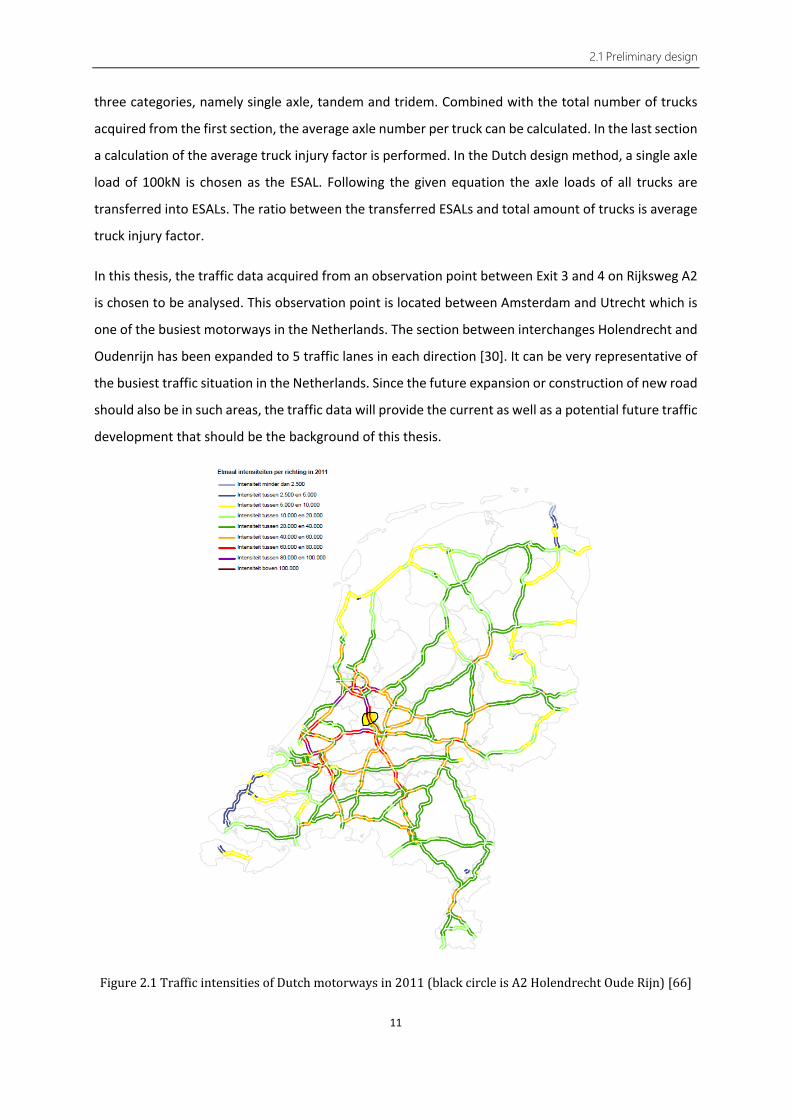
Table 2.1 Data analysis for daily traffic flow between Exit 3 and 4 on Rijksweg A2
From the first file it can be easily observed that the traffic flow does not distribute over the lanes evenly.
Generally speaking, the outside lanes (Lane 3, 4 & 5) bear more traffic flow than inside ones (Lane 1 &
2). Further calculation shows that different types of vehicles also distribute differently over 5 lanes. To
be specific, the majority of heavy trucks run on the most outside lane (Lane 5) while light trucks run
mainly on both Lane 4 and 5. On contrary, when considering the “10000 rule”, the passenger cars more
or less spread evenly over 5 lanes.
In most of the pavement design methods, the impact of the passenger cars to the pavement is usually
neglected. It is commonly agreed that the impact of 10,000 passenger cars can be simply considered
equal to the impact caused by 1 truck [31]. Even if there are 100,000 passenger cars per day per
2.1 Preliminary design
13
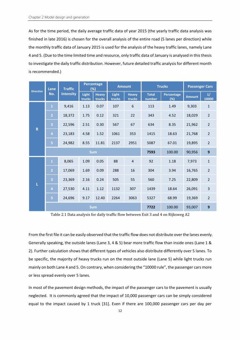
direction, when they are transformed into trucks, which is 10 per day, the number is so small that can
be neglected comparing to the huge daily truck flow. In the Dutch design method, only axles with a
load more than 20kN are counted. Therefore in the second file, the distribution of single axle loads on
Lane 4 and 5 is exhibited. For both directions, approximately 75% of the axles are running on the Lane
5 while the other 25% are taken by Lane 4.
Direction Lane No. ESALs Percentage
R
4 302,281 24.05%
5 954,741 75.95%
Total 1,257,022
L
4 346,456 24.91%
5 1,044,552 75.09%
Total 1,391,008
Table 2.2 Daily ESALs distribution on lane 4 and 5 between Exit 3 and 4 on Rijksweg A2
2.1.2. Thickness design by the Dutch standard software
Ontwerpinstrumentarium asfaltverhardingen (OIA) is the latest standard software for asphalt
pavement design in the Netherlands based on the new design code of Rijkswaterstaat [32]. It is widely
used by Dutch contractors to evaluate new designed pavements. OIA will provide an adequate
thickness design for all the layers in the pavement structure based on a given input. As discussed earlier
in chapter 1.2.4, in OIA, when there are more than 3 lanes in each direction, in this case 5 lanes, the
right hand lane will be chosen as design lane and assigned 90% of the total traffic volume. To reduce
the thickness of lower traffic lanes, the pavement thickness design should be performed individually
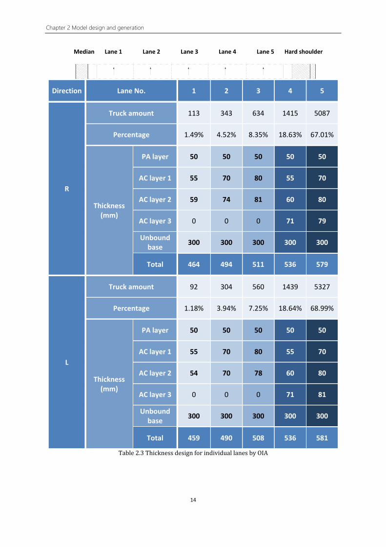
for each lane. With the traffic data analysed in chapter 2.1.1, the thickness design for each lane can be
addressed via OIA according to its own traffic volume. The results are shown below and indicate that
there is indeed a great potential of reduction in asphalt layers’ thickness.
Chapter 2 Model design and generation
14
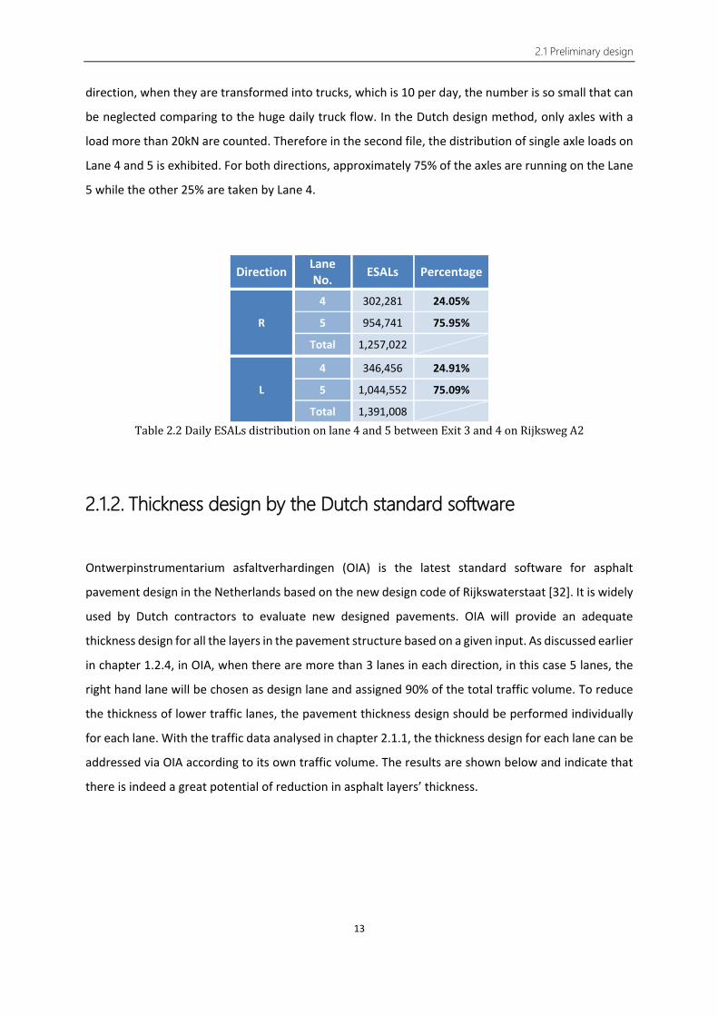
Direction Lane No. 1 2 3 4 5
R
Truck amount 113 343 634 1415 5087
Percentage 1.49% 4.52% 8.35% 18.63% 67.01%
Thickness (mm)
PA layer 50 50 50 50 50
AC layer 1 55 70 80 55 70
AC layer 2 59 74 81 60 80
AC layer 3 0 0 0 71 79
Unbound base 300 300 300 300 300
Total 464 494 511 536 579
L
Truck amount 92 304 560 1439 5327
Percentage 1.18% 3.94% 7.25% 18.64% 68.99%
Thickness (mm)
PA layer 50 50 50 50 50
AC layer 1 55 70 80 55 70
AC layer 2 54 70 78 60 80
AC layer 3 0 0 0 71 81
Unbound base 300 300 300 300 300
Total 459 490 508 536 581
Table 2.3 Thickness design for individual lanes by OIA
Median Lane 1 Lane 2 Lane 3 Lane 4 Lane 5 Hard shoulder

2.1 Preliminary design
15
A stair-step shaped design can be easily established based on the individual lane layer thickness
calculations. To ensure an even surface, a reversed stair structure is proposed by accordingly increasing
the thickness of unbound base layer of each lane. However, it can also be easily predicted that a severe
stress concentration may occur at the edges (see the red circles in figure 2.2). Ideally smoother (curved)
transitions should be placed between two lanes, however this solution is neither practicable nor
economical from the construction perspective. Therefore, a slope shaped design is proposed in this
thesis.
Figure 2.2 Development of the new pavement structural design
Lane 1 Lane 2 Lane 3 Lane 4 Lane 5
Sta
ir Re
vers
ed
Stai
r Sl
ope

Chapter 2 Model design and generation
16
2.2. Model design
As discussed in chapter 1, all the current pavement design methods are based on a parallel multi-layer
structure assumption, so is the design software. In section 2.1, a slope shaped new design has been
proposed, which contains un-parallel layers. Hence traditional design methods are no longer applicable
here. As a result, a finite element method (FEM) is introduced in this thesis. A FEM software, CAPA-3D,
is used for the strain and stress calculation as well as long-term deformation simulations.
CAPA-3D is a three dimensional finite elements based research tool [33]. Like all the FEM software, the
run time and the calculation precision are highly influenced by the dimension and fineness of the mesh.
The bigger and finer a mesh is, the longer run time it will take and produce a more precise result.
Therefore a proper model has to be established to gain a balance between time consumption and
precision of the results.
2.2.1. Number of lanes and dimensions
The Handboek wegontwerp is a design manual published by CROW. It provides guidelines for traffic
facilities design outside urban areas in the Netherlands. In its first part, Basiscriteria, a standard layout
of a stroomweg (Dutch motorway) is presented, which contains 2 lanes per direction with 1 emergency
lane [34].
Figure 2.3 Typical dimension design for a Dutch 2×2 motorway [34]

2.2 Model design
17
In the previous chapter the traffic data of a 2×5-lane road was used for analysis. However, the scale of
a 2×5-lane road plus 1 additional emergency lane can be too time consuming for the finite elements
analysis, also the 5-lane motorways do exist in the Netherlands but they are not the standard. Instead,
a 2×3-lane layout is proposed. This model not only represents the light and heavy truck traffic lanes,
but also provides an overall view of the strain and stress condition along the entire road cross section
by adding a passenger car lane and emergency lane. The total transverse width of the model is 15
metres.
A road can be seen as an infinite structure in the longitudinal direction. Thus for a finite element model
the length ceiling also should be limited. In addition, a minimum length also has to be determined to
minimize the edge effect. Several simple trials were performed during the preliminary research. The
results show that for a typical tyre print the influence area for strain and stress of under layers is within
5 metres diameter. Therefore a model with the length of 6 metres in the direction of traffic was
selected such that one full passage of the truck on the pavement can be achieved to obtain a complete
longitudinal tensile strain response curve including the expected compression-tension-compression
sequence [35] which will be further discussed in the next chapter.
Median Lane 1 Lane2 Lane 3 Hard shoulder
Figure 2.4 Dimension design of the model (Top view, m)
Redresseerstrook Marker Marker Redresseerstrook Edge
1,1 0,8 3,25 3,25 0,8 1,65
1,9 10,15 2,95
15
6
0,53,25
0,2 0,2
Chapter 2 Model design and generation
18
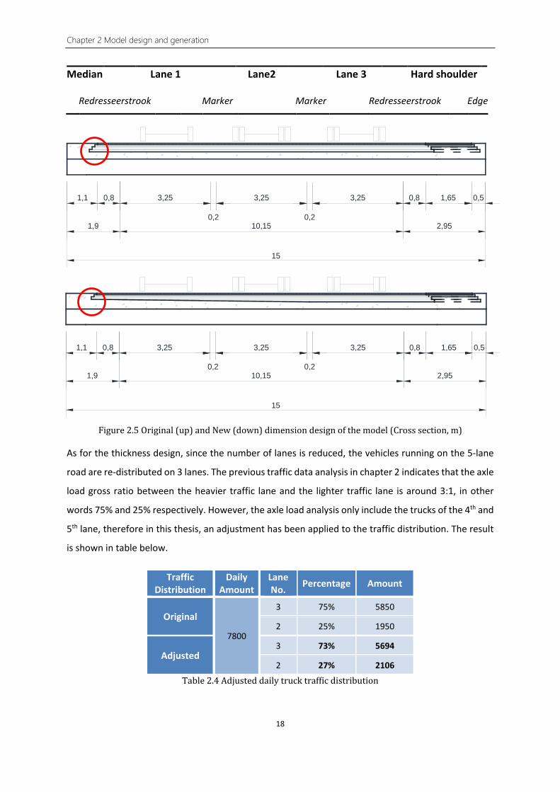
Median Lane 1 Lane2 Lane 3 Hard shoulder
Figure 2.5 Original (up) and New (down) dimension design of the model (Cross section, m)
As for the thickness design, since the number of lanes is reduced, the vehicles running on the 5-lane
road are re-distributed on 3 lanes. The previous traffic data analysis in chapter 2 indicates that the axle
load gross ratio between the heavier traffic lane and the lighter traffic lane is around 3:1, in other
words 75% and 25% respectively. However, the axle load analysis only include the trucks of the 4th and
5th lane, therefore in this thesis, an adjustment has been applied to the traffic distribution. The result
is shown in table below.
Traffic Distribution
Daily Amount
Lane No. Percentage Amount
Original
7800
3 75% 5850
2 25% 1950
Adjusted 3 73% 5694
2 27% 2106
Table 2.4 Adjusted daily truck traffic distribution
Redresseerstrook Marker Marker Redresseerstrook Edge
1,1 0,8 3,25 3,25 0,8 1,65
1,9 10,15 2,95
15
0,53,25
0,2 0,2
1,1 0,8 3,25 3,25 0,8 1,65
1,9 10,15 2,95
15
0,53,25
0,2 0,2

2.2 Model design
19
Comparing the new traffic data to the original data used in the software design, an approximation of
the asphalt layer thickness can be estimated. The final thickness design for the heavy traffic lane is
composed of one PA layer (50mm), three AC layers (75mm, 80mm and 80mm), one unbound subbase
layer (300mm) and one subgrade layer. 50
235
300
500
Figure 2.6 Pavement layer thickness design (mm)
The boundary conditions are also required to be determined in advance. It is assumed that there is
neither vertical nor horizontal movement at the bottom of the finite elements model, hence the
bottom of the model was completely restrained. As to the four vertical surfaces, their horizontal
movement perpendicular to the perimeters is also restrained whilst the remaining two directions were
considered free, in other words each vertical surface is given two degrees of freedom. In total there
are 7 restraints applied to the model. According to the Dutch design method [23], all the layers in the
pavement are considered fully bounded, which means the interfaces between different layers are
assumed to be tied together without any relative movement.
To optimize a balance between time consumption and result precision, a reasonably refined mesh
should be found. The model is divided into several finer mesh parts close to the loading area and
coarser mesh parts away from it. Analogously, the area required to produce more output data is also
finer than others, for instance, the upper layers, namely the asphalt layers, are divided into more sub
layers than the lower substructure.
The final model has a dimension of 15 m × 6 m × 1.085 m with a mesh of 46,000 elements (66 super
elements). By calculation the new pavement structure will save approximately 10% of the AC material.
PA AC (75+80+80) Mixed granules Sand

Chapter 2 Model design and generation
20
Figure 2.7 Super elements and slope creation
Figure 2.8 Final mesh of original design
Figure 2.9 Final mesh of new design
2.2.2. Materials
In the Dutch design method, all construction materials are treated as elastic solids, including asphalt
[23], although in reality asphalt materials behave viscoelastically. Many pavement analysis methods
Reduced part
Original design (Paralleled) New design (Slope)
1 11
66

2.2 Model design
21
have been developed based upon the viscoelastic characterization of asphalt material to calculate
strain response and deformation. In this thesis, a rutting calculation following the American standard
(Mechanistic-Empirical Pavement Design Guide, MEPDG) is performed for comparison. It requires the
introduction of viscoelasticity to the asphalt material.
The viscoelasticity of asphalt can be simply seen as a time-dependent behaviour between stress and
strain. The key to simulate the real behaviour of asphalt materials is a proper model of their stress-
strain relationship, which can be simulated by a mechanical model consisting of elastic components
(spring) and viscous components (dashpot). In CAPA-3D, a Generalized Maxwell model, also known as
Wiechert model [36], is employed. It is composed of one single spring and multiple Maxwell
components connected in parallel as shown in figure 2.10. Each spring is assigned a relaxation modulus
E while each dashpot is assigned a frictional resistance η. The modulus of the Generalized Maxwell
model can be expressed as below.
Figure 2.10 Generalized Maxwell model [37]
𝐺𝐺′(𝜔𝜔) = 𝐺𝐺∞ + �𝜔𝜔2𝜏𝜏𝑖𝑖2𝐺𝐺𝑖𝑖𝜔𝜔2𝜏𝜏𝑖𝑖2 + 1
𝑁𝑁
𝑖𝑖=1
(2.1) Where,
𝐺𝐺′(𝜔𝜔) = Storage modulus (Pa)
𝐺𝐺∞ = Long term modulus (Pa)
𝑁𝑁 = Relaxation modes (-)
𝜔𝜔 = Angular frequency (rad/s)
𝜏𝜏𝑖𝑖 = Relaxation time (s)
𝐺𝐺𝑖𝑖 = Prony coefficients (Pa)

Chapter 2 Model design and generation
22
Equation 2.1 is also known as Prony series [38]. In this thesis, two viscoelastic materials are used,
namely porous asphalt (PA) and asphalt concrete (AC). Both materials are tested in the laboratory and
translated into stiffness master curves. In CAPA-3D, the Prony series are converted into 4 parameters
to represent the material properties.
𝜇𝜇 = 𝐺𝐺∗ (2.2)
𝜆𝜆 = 2𝜈𝜈1−2𝜈𝜈
𝐺𝐺∗ (2.3)
𝜂𝜂 = 𝜏𝜏𝜏𝜏 = 2𝜏𝜏𝐺𝐺∗(1 + 𝜈𝜈) (2.4)
𝜂𝜂𝑣𝑣𝑣𝑣𝑣𝑣 = 𝜂𝜂𝑑𝑑𝑑𝑑𝑣𝑣 = 49𝜂𝜂 (2.5)
Where,
𝜇𝜇,𝐺𝐺∗ = Shear modulus (Pa)
𝜆𝜆 = Lamé's first parameter (Pa)
𝜈𝜈 = Poisson’s ratio (-), set to 0.35
𝜏𝜏 = Relaxition time (s)
𝜂𝜂, 𝜂𝜂𝑣𝑣𝑣𝑣𝑣𝑣 & 𝜂𝜂𝑑𝑑𝑑𝑑𝑣𝑣 = Viscosity parameters (Pas)
By substituting the data into equation 2.1 to 2.5, the Prony series of the two materials can be obtained.
𝒊𝒊 τ (s)
Gi (Pa)
ν (-)
μ (Pa)
λ (Pa)
E (Pa)
η (Pas)
ηd (Pas)
ηv (Pas)
1 2.12E-01 3.50E+09 3.50E-01 1.32E+09 3.09E+09 3.58E+09 7.57E+08 3.36E+08 3.36E+08
2 2.18E-04 2.44E+09 3.50E-01 5.45E+09 1.27E+10 1.47E+10 3.21E+06 1.43E+06 1.43E+06
3 3.96E-06 2.44E+09 3.50E-01 2.99E+09 6.97E+09 8.07E+09 3.19E+04 1.42E+04 1.42E+04
4 2.12E-07 2.44E+09 3.50E-01 2.99E+09 6.97E+09 8.07E+09 1.71E+03 7.62E+02 7.62E+02
5 5.92E-03 2.10E+09 3.50E-01 2.74E+09 6.40E+09 7.40E+09 4.38E+07 1.95E+07 1.95E+07
∞ 7.10E+03 3.50E-01 2.95E+02 6.87E+02 7.95E+02
Table 2.5 Material parameters (Prony series) of porous asphalt (PA)

2.2 Model design
23
𝒊𝒊 τ (s)
Gi (Pa)
ν (-)
μ (Pa)
λ (Pa)
E (Pa)
η (Pas)
ηd (Pas)
ηv (Pas)
1 2.44E-02 2.44E+09 3.50E-01 2.44E+09 5.70E+09 6.60E+09 1.61E+08 7.15E+07 7.15E+07
2 4.19E-03 2.44E+09 3.50E-01 2.44E+09 5.70E+09 6.60E+09 2.77E+07 1.23E+07 1.23E+07
3 1.19E-01 2.44E+09 3.50E-01 2.44E+09 5.70E+09 6.60E+09 7.88E+08 3.50E+08 3.50E+08
4 2.23E-01 2.10E+09 3.50E-01 2.10E+09 4.89E+09 5.66E+09 1.26E+09 5.62E+08 5.62E+08
5 1.38E-02 1.56E+09 3.50E-01 1.56E+09 3.65E+09 4.22E+09 5.85E+07 2.60E+07 2.60E+07
6 4.19E-03 8.83E+06 3.50E-01 8.83E+06 2.06E+07 2.38E+07 9.99E+04 4.44E+04 4.44E+04
∞ 4.28E+09 3.50E-01 4.28E+10 1.00E+11 1.16E+11
Table 2.6 Material parameters (Prony series) of asphalt concrete (AC)
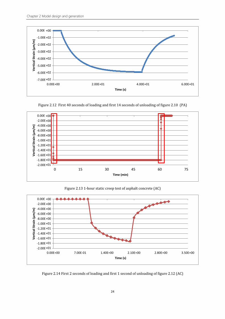
A static creep test is done in CAPA-3D. The specimen is a 100×100×100 mm3 cube. A 200 MPa load is
applied onto the specimen for 1 hour. At the end of that 1 hour, the load is removed to allow the
specimen to rebound for 10 minutes [39]. The creep test results are shown in figure 2.11–2.14. It can
be witnessed that the two material models do show a time-dependent strain-stress behaviour and are
capable of representing the viscoelasticity of the asphalt materials.
Figure 2.11 1-hour static creep test of porous asphalt (PA)
-7.00E-04
-6.00E-04
-5.00E-04
-4.00E-04
-3.00E-04
-2.00E-04
-1.00E-04
0.00E+00
0.00E+00 9.00E+02 1.80E+03 2.70E+03 3.60E+03 4.50E+03
Vert
ical
Str
ain
(μm
/m)
Time (min)0 15 30 45 60 75
+00
+02
+02
+02
+02
+02
+02
+02
Chapter 2 Model design and generation
24
Figure 2.12 First 40 seconds of loading and first 14 seconds of unloading of figure 2.10 (PA)
Figure 2.13 1-hour static creep test of asphalt concrete (AC)
Figure 2.14 First 2 seconds of loading and first 1 second of unloading of figure 2.12 (AC)
-7.00E-04
-6.00E-04
-5.00E-04
-4.00E-04
-3.00E-04
-2.00E-04
-1.00E-04
0.00E+00
0.00E+00 2.00E+01 4.00E+01 6.00E+01
Vert
ical
Str
ain
(μm
/m)
Time (s)
-2.00E-05-1.80E-05-1.60E-05-1.40E-05-1.20E-05-1.00E-05-8.00E-06-6.00E-06-4.00E-06-2.00E-060.00E+00
0.00E+00 9.00E+02 1.80E+03 2.70E+03 3.60E+03 4.50E+03
Vert
ical
Str
ain
(μm
/m)
Time (min)
-2.00E-05-1.80E-05-1.60E-05-1.40E-05-1.20E-05-1.00E-05-8.00E-06-6.00E-06-4.00E-06-2.00E-060.00E+00
0.00E+00 7.00E-01 1.40E+00 2.10E+00 2.80E+00 3.50E+00
Vert
ical
Str
ain
(μm
/m)
Time (s)
0 15 30 45 60 75
+00
+02
+02
+02
+02
+02
+02
+02
+00 +00 +00 +00 +00 +01 +01 +01 +01 +01 +01
+00 +00 +00 +00 +00 +01 +01 +01 +01 +01 +01

2.2 Model design
25
2.2.3. Tire prints
In The Dutch design method, four types of tires can be used for design calculation, namely single tire
(EL), dual tire (DL), broadband (BB) and super broadband (SB). The nominal dimensions of the contact
area of these four tires are determined. The dimension of a tire print depends on the load that is
exerted on it. For all the different loads, the width of the tire print remains substantially constant while
the length changes correspondingly [23]. The following procedure is used to determine the rectangular
contact area of a tire under a certain load. In OIA, the rectangular contact area is then converted into
an equivalent circular area for the strain calculation. However, in CAPA-3D, a rectangular shaped load
is much easier to apply and more accurate to the real contact condition. Therefore in this thesis the
last step of conversion is abandoned.
𝐴𝐴𝑏𝑏𝑏𝑏𝑏𝑏𝑑𝑑 = 𝛽𝛽 ∙ 1000 ∙ 𝐹𝐹𝑏𝑏𝑣𝑣𝑛𝑛𝑛𝑛𝑏𝑏𝑣𝑣 𝜎𝜎𝑏𝑏𝑣𝑣𝑛𝑛𝑛𝑛𝑏𝑏𝑣𝑣� (2.6)
Where,
𝐴𝐴𝑏𝑏𝑏𝑏𝑏𝑏𝑑𝑑 = Contact area of the tire (mm2)
𝛽𝛽 = Factor depending on the load
𝐹𝐹𝑏𝑏𝑣𝑣𝑛𝑛𝑛𝑛𝑏𝑏𝑣𝑣 = Normal tire load (kN)
𝜎𝜎𝑏𝑏𝑣𝑣𝑛𝑛𝑛𝑛𝑏𝑏𝑣𝑣 = Normal pressure (MPa)
Single tire (EL)
Dual tire (DL)
Broadband (BB)
Super Broadband (SB)
Normal axle load (kN) 70 120 100 115 Normal wheel load (kN) 35 30 50 57.5
Wheel width (mm) 200 200 300 400 Normal contact pressure
(MPa) 0.75 0.8 0.85 0.95
Centre-to-centre distance (mm)
315
Table 2.7 Tire types and contact area data
The actual load of individual tire for single tire (EL), broadband (BB) or super broadband (SB) is
determined using equation 2.7:
𝐹𝐹𝑏𝑏𝑏𝑏𝑏𝑏𝑑𝑑 = 0.5 ∙ 𝐹𝐹𝑏𝑏𝑎𝑎𝑣𝑣𝑑𝑑,𝑖𝑖 (2.7)
Where,
𝐹𝐹𝑏𝑏𝑏𝑏𝑏𝑏𝑑𝑑 = Actual tire load (kN)

Chapter 2 Model design and generation
26
𝐹𝐹𝑏𝑏𝑎𝑎𝑣𝑣𝑑𝑑,𝑖𝑖 = Design value of the single axle load of axle load class 𝑖𝑖 (kN)
The actual load of individual tire for dual tire (DL) is determined using equation 2.8:
𝐹𝐹𝑏𝑏𝑏𝑏𝑏𝑏𝑑𝑑 = 0.25 ∙ 𝐹𝐹𝑏𝑏𝑎𝑎𝑣𝑣𝑑𝑑,𝑖𝑖 (2.8)
Where,
𝐹𝐹𝑏𝑏𝑏𝑏𝑏𝑏𝑑𝑑 = Actual tire load (kN)
𝐹𝐹𝑏𝑏𝑎𝑎𝑣𝑣𝑑𝑑,𝑖𝑖 = Design value of the single axle load of axle load class 𝑖𝑖 (kN)
The factor 𝛽𝛽 is determined by equation 2.9:
𝛽𝛽 = 1 + 0.59454 ∙ 𝐵𝐵𝑑𝑑𝑒𝑒 − 0.10182 ∙ 𝐵𝐵𝑑𝑑𝑒𝑒2 (2.9)
Where,
𝛽𝛽 = Factor determined by the load (-)
𝐵𝐵𝑑𝑑𝑒𝑒 = Equivalent load (-)
For the determination of equivalent load:
𝐵𝐵𝑑𝑑𝑒𝑒 = 𝐹𝐹𝑏𝑏𝑏𝑏𝑏𝑏𝑏𝑏𝐹𝐹𝑏𝑏𝑛𝑛𝑛𝑛𝑛𝑛𝑏𝑏𝑛𝑛
− 1 (2.10)
Where,
𝐵𝐵𝑑𝑑𝑒𝑒 = Equivalent load (-)
𝐹𝐹𝑏𝑏𝑏𝑏𝑏𝑏𝑑𝑑 = Actual tire load (kN)
𝐹𝐹𝑏𝑏𝑣𝑣𝑛𝑛𝑛𝑛𝑏𝑏𝑣𝑣 = Normal tire load (kN)
Hence the contact pressure can be determined:
𝜎𝜎𝑏𝑏𝑏𝑏𝑏𝑏𝑑𝑑 = 𝐹𝐹𝑏𝑏𝑏𝑏𝑏𝑏𝑏𝑏𝐴𝐴𝑏𝑏𝑏𝑏𝑏𝑏𝑏𝑏
(2.11)
Where,
𝜎𝜎𝑏𝑏𝑏𝑏𝑏𝑏𝑑𝑑 = Actual contact pressure (MPa)
𝐹𝐹𝑏𝑏𝑏𝑏𝑏𝑏𝑑𝑑 = Actual tire load (kN)
𝐴𝐴𝑏𝑏𝑏𝑏𝑏𝑏𝑑𝑑 = Contact area of the tire (mm2)
OIA provides several standard axle load spectra according to the Dutch road design guide, as well as
tire band spectra. For the motorway design, the heavy axle load spectrum of Rijkswaterstaat has been

2.2 Model design
27
chosen for the analysis [32]. All the axle loads are divided into 10 tonnage classes. A standard tire type
spectrum is also chosen, in which only 3 out of 4 tire types occur.
Range Calculation value %
20-40 30 15.60
40-60 50 27.10
60-80 70 28.10
80-100 90 14.60
100-120 110 8.75
120-140 130 4.60
140-160 150 1.04
160-180 170 0.13
180-200 190 0.08
200-220 210 0.00
Table 2.8 Axle load spectrum
Tire type %
Single tire (EL) 39.00
Dual tire (DL) 38.00
Broadband (BB) 23.00
Super Broadband (SB) 0.00
Table 2.9 Tire type spectrum
As a result, there are a total of 30 different tire prints that are used in this thesis. An additional single
tire (EL) print for passenger cars is also determined. A summary form is displayed down below.

Chapter 2 Model design and generation
28
Design value (kN) Singe tire (EL) Dual tire (DL) Broadband (BB)
per axle
per tire (EL/BB)
per tire (DL)
A (mm2)
σ (MPa)
L (mm)
A (mm2)
σ (MPa)
L (mm)
A (mm2)
σ (MPa)
L (mm)
30 15 7.5 29261 0.51 146.30 18631 0.40 93.15 31408 0.48 104.69
50 25 12.5 38352 0.65 191.76 23195 0.54 115.98 39840 0.63 132.80
70 35 17.5 46667 0.75 233.33 27547 0.64 137.74 47793 0.73 159.31
90 45 22.5 54206 0.83 271.03 31688 0.71 158.44 55266 0.81 184.22
110 55 27.5 60970 0.90 304.85 35616 0.77 178.08 62261 0.88 207.54
130 65 32.5 66957 0.97 334.79 39331 0.83 196.66 68776 0.95 229.25
150 75 37.5 72169 1.04 360.85 42835 0.88 214.18 74813 1.00 249.38
170 85 42.5 76606 1.11 383.03 46127 0.92 230.63 80370 1.06 267.90
190 95 47.5 80266 1.18 401.33 49206 0.97 246.03 85448 1.11 284.83
210 105 52.5 83151 1.26 415.75 52074 1.01 260.37 90047 1.17 300.16
7.5 3.75 1.875 18106 0.21 90.53
Tread width (mm) 200 200 300 Table 2.10 Tire prints summary
2.2.4. Axle tracks
Axle track is the distance between the centreline of two wheels (for dual tire the centreline in the
middle of one dual tire set is used) on the same axle. It varies with the vehicle types, loads and in some
cases the position (front or rear track) of the axle. For the traffic input a standard axle track need to be
determined.
In Handboek wegontwerp the average dimensions of different vehicle classes are specified for the
purpose of road design [34]. The average axle track of a passenger car is 1.50 m whilst a truck holds a
larger axle track of 2.15 m (figure 2.14).
Figure 2.15 Average dimensions of passenger cars (r) and trucks (l) [34]

2.2 Model design
29
However, the trucks used for pavement design, as discussed in the section 2.2.3, are equipped with
three tire types which will result in different axle tracks. The Handboek wegontwerp also provides a
standard width of a truck (2.62m). Hence the axle tracks of three tire types can be determined. The
results are shown in table 2.11.
Passenger car
Truck
EL DL BB
Axle track (mm) 1500 2100 1785 2000
Table 2.11 Axle tracks
2.2.5. Time interval
In most situations, vehicles apply moving, dynamic load onto the pavement. Obviously it is a
continuous process. However, in finite element software, this continuous process is simulated by a
series of patterns gradually shifted according to time. It takes a fixed time for a wheel to pass a certain
distance, in this case 6 metres, at a certain speed. Therefore the more steps there are, the shorter
interval it will need, and obviously the simulation will be closer to a continuous moving load. On the
other hand, the more steps, the more computing time. Thus an optimized balance between running
time and result precision should also be found. 5 tests with different time intervals were performed
during the preliminary research. It is set that for a test with 2N time steps, the wheel centre will come
to the position right on the output point at the (N+1)th step. The results are shown down below. The
red bold values are the maximum strain values occurred in each test.

Chapter 2 Model design and generation
30
PA layer
Total time steps
Output time step Time (s)
Strain (μm/m)
xx yy zz
10 5 1.29E-01 -1.84E+01 6.83E+00 2.49E+00
6 1.54E-01 -4.42E+01 -1.22E+02 -4.50E+01
20
10 1.28E-01 -3.33E+01 2.13E+01 -1.66E+01
11 1.41E-01 -4.74E+01 -9.45E+01 -4.66E+01
12 1.54E-01 -4.02E+01 -1.52E+01 -2.43E+01
40
20 1.29E-01 -3.76E+01 -3.58E+01 -1.89E+01
21 1.35E-01 -4.27E+01 -8.76E+01 -3.84E+01
22 1.41E-01 -4.18E+01 -4.89E+01 -4.58E+01
23 1.48E-01 -3.67E+01 -1.80E+01 -2.42E+01
80
40 1.29E-01 -4.05E+01 -6.64E+01 -3.55E+01
41 1.32E-01 -4.26E+01 -8.33E+01 -4.12E+01
42 1.35E-01 -4.30E+01 -1.01E+02 -3.27E+01
43 1.38E-01 -4.19E+01 -5.92E+01 -4.44E+01
44 1.41E-01 -4.01E+01 -2.65E+01 -3.26E+01
160
80 1.29E-01 -4.16E+01 -7.27E+01 -3.92E+01
81 1.30E-01 -4.25E+01 -8.12E+01 -4.14E+01
82 1.32E-01 -4.30E+01 -8.94E+01 -4.13E+01
83 1.33E-01 -4.30E+01 -9.88E+01 -3.43E+01
84 1.35E-01 -4.27E+01 -1.03E+02 -3.06E+01
85 1.37E-01 -4.20E+01 -6.66E+01 -4.29E+01
86 1.38E-01 -4.11E+01 -3.76E+01 -4.07E+01
87 1.40E-01 -4.01E+01 -2.88E+01 -3.32E+01
Table 2.12 Peak strain values for different time intervals (PA layer, Broadband, 210 kN axle load)
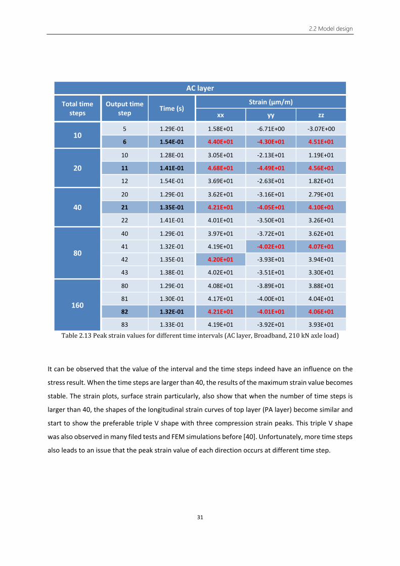
2.2 Model design
31
AC layer
Total time steps
Output time step Time (s)
Strain (μm/m)
xx yy zz
10 5 1.29E-01 1.58E+01 -6.71E+00 -3.07E+00
6 1.54E-01 4.40E+01 -4.30E+01 4.51E+01
20
10 1.28E-01 3.05E+01 -2.13E+01 1.19E+01
11 1.41E-01 4.68E+01 -4.49E+01 4.56E+01
12 1.54E-01 3.69E+01 -2.63E+01 1.82E+01
40
20 1.29E-01 3.62E+01 -3.16E+01 2.79E+01
21 1.35E-01 4.21E+01 -4.05E+01 4.10E+01
22 1.41E-01 4.01E+01 -3.50E+01 3.26E+01
80
40 1.29E-01 3.97E+01 -3.72E+01 3.62E+01
41 1.32E-01 4.19E+01 -4.02E+01 4.07E+01
42 1.35E-01 4.20E+01 -3.93E+01 3.94E+01
43 1.38E-01 4.02E+01 -3.51E+01 3.30E+01
160
80 1.29E-01 4.08E+01 -3.89E+01 3.88E+01
81 1.30E-01 4.17E+01 -4.00E+01 4.04E+01
82 1.32E-01 4.21E+01 -4.01E+01 4.06E+01
83 1.33E-01 4.19E+01 -3.92E+01 3.93E+01
Table 2.13 Peak strain values for different time intervals (AC layer, Broadband, 210 kN axle load)
It can be observed that the value of the interval and the time steps indeed have an influence on the
stress result. When the time steps are larger than 40, the results of the maximum strain value becomes
stable. The strain plots, surface strain particularly, also show that when the number of time steps is
larger than 40, the shapes of the longitudinal strain curves of top layer (PA layer) become similar and
start to show the preferable triple V shape with three compression strain peaks. This triple V shape
was also observed in many filed tests and FEM simulations before [40]. Unfortunately, more time steps
also leads to an issue that the peak strain value of each direction occurs at different time step.
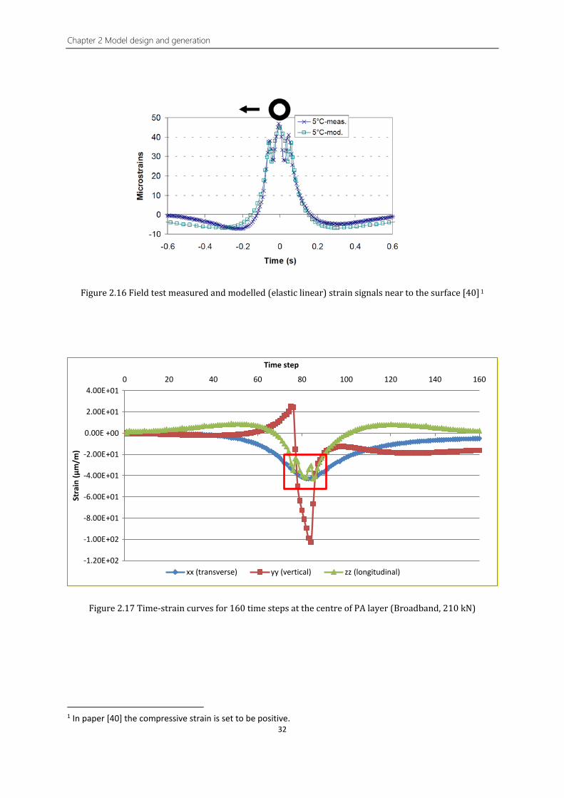
Chapter 2 Model design and generation
32
Figure 2.16 Field test measured and modelled (elastic linear) strain signals near to the surface [40] 1
Figure 2.17 Time-strain curves for 160 time steps at the centre of PA layer (Broadband, 210 kN)
1 In paper [40] the compressive strain is set to be positive.
-1.20E-04
-1.00E-04
-8.00E-05
-6.00E-05
-4.00E-05
-2.00E-05
0.00E+00
2.00E-05
4.00E-050 20 40 60 80 100 120 140 160
Stra
in (μ
m/m
)
Time step
xx (transverse) yy (vertical) zz (Longitudinal)(longitudinal)
+01
+01
+00
+01
+01
+01
+01
+02
+02
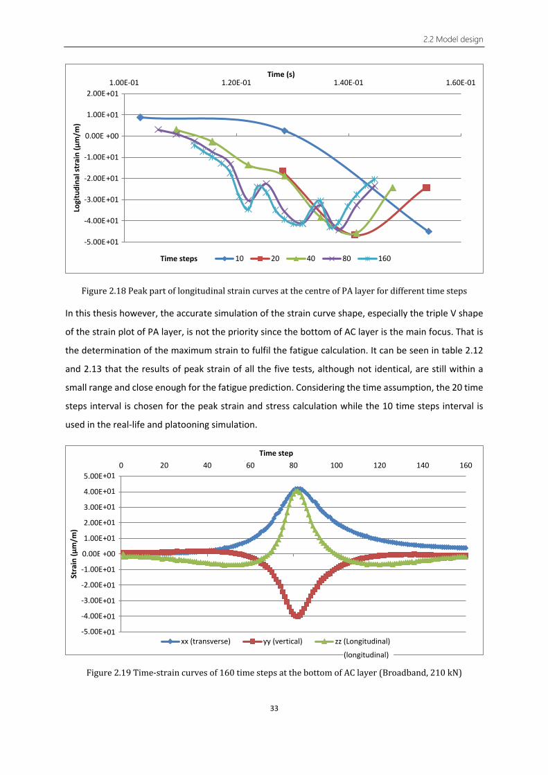
2.2 Model design
33
Figure 2.18 Peak part of longitudinal strain curves at the centre of PA layer for different time steps
In this thesis however, the accurate simulation of the strain curve shape, especially the triple V shape
of the strain plot of PA layer, is not the priority since the bottom of AC layer is the main focus. That is
the determination of the maximum strain to fulfil the fatigue calculation. It can be seen in table 2.12
and 2.13 that the results of peak strain of all the five tests, although not identical, are still within a
small range and close enough for the fatigue prediction. Considering the time assumption, the 20 time
steps interval is chosen for the peak strain and stress calculation while the 10 time steps interval is
used in the real-life and platooning simulation.
Figure 2.19 Time-strain curves of 160 time steps at the bottom of AC layer (Broadband, 210 kN)
-5.00E-05
-4.00E-05
-3.00E-05
-2.00E-05
-1.00E-05
0.00E+00
1.00E-05
2.00E-051.00E-01 1.20E-01 1.40E-01 1.60E-01
Logi
tudi
nal s
trai
n (μ
m/m
)Time (s)
10 20 40 80 160
-5.00E-05
-4.00E-05
-3.00E-05
-2.00E-05
-1.00E-05
0.00E+00
1.00E-05
2.00E-05
3.00E-05
4.00E-05
5.00E-050 20 40 60 80 100 120 140 160
Stra
in (μ
m/m
)
Time step
xx (transverse) yy (vertical) zz (Longitudinal)
Time steps
(longitudinal)
+01
+01
+00
+01
+01
+01
+01
+01
+01
+01
+01
+01
+01
+00
+01
+01
+01
+01
+01
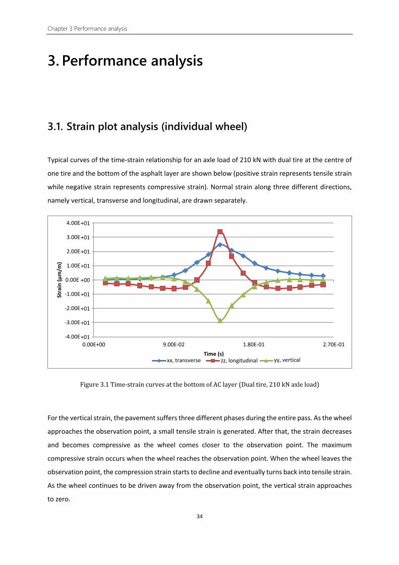
Chapter 3 Performance analysis
34
3. Performance analysis
3.1. Strain plot analysis (individual wheel)
Typical curves of the time-strain relationship for an axle load of 210 kN with dual tire at the centre of
one tire and the bottom of the asphalt layer are shown below (positive strain represents tensile strain
while negative strain represents compressive strain). Normal strain along three different directions,
namely vertical, transverse and longitudinal, are drawn separately.
Figure 3.1 Time-strain curves at the bottom of AC layer (Dual tire, 210 kN axle load)
For the vertical strain, the pavement suffers three different phases during the entire pass. As the wheel
approaches the observation point, a small tensile strain is generated. After that, the strain decreases
and becomes compressive as the wheel comes closer to the observation point. The maximum
compressive strain occurs when the wheel reaches the observation point. When the wheel leaves the
observation point, the compression strain starts to decline and eventually turns back into tensile strain.
As the wheel continues to be driven away from the observation point, the vertical strain approaches
to zero.
-4.00E-05
-3.00E-05
-2.00E-05
-1.00E-05
0.00E+00
1.00E-05
2.00E-05
3.00E-05
4.00E-05
0.00E+00 9.00E-02 1.80E-01 2.70E-01
Stra
in (μ
m/m
)
Time (s)xx zz yyxx, transverse yy, vertical zz, longitudinal
+01
+01
+01
+01
+00
+01
+01
+01
+01

3.1 Strain plot analysis (individual wheel)
35
Figure 3.2 Time-vertical strain curve at the bottom of AC layer (Dual tire, 210 kN)
For the longitudinal strain, a similar pattern can be obtained, only the directions of the strain are
reversed. Instead, a compression-tension-compression pattern is observed [41]. Also these three
segments of the curve are more distinctive with a larger deviation between the tensile and
compressive strain comparing to the vertical strain curve. This pattern was investigated by Sebaaly and
Mamlouk [42]. They developed a pavement structural model that takes into account the inertial forces.
The result shown that the vertical acceleration of a point within the pavement changes from positive
to negative as the axle loading passes over. There is also a simpler explanation that the compressive
longitudinal strain is a result of the combination of bending stresses and horizontal shear stresses.
Figure 3.3 Time-longitudinal strain curve at the bottom of AC layer (Dual tire, 210 kN)
-3.50E-05
-3.00E-05
-2.50E-05
-2.00E-05
-1.50E-05
-1.00E-05
-5.00E-06
0.00E+00
5.00E-06
0.00E+00 9.00E-02 1.80E-01 2.70E-01
Stra
in (μ
m/m
)
Time (s)
-1.00E-05
-5.00E-06
0.00E+00
5.00E-06
1.00E-05
1.50E-05
2.00E-05
2.50E-05
3.00E-05
3.50E-05
4.00E-05
0.00E+00 9.00E-02 1.80E-01 2.70E-01
Stra
in (μ
m/m
)
Time (s)
+00
+00
+00
+01
+01
+01
+01
+01
+01
+01
+01
+01
+01
+01
+01
+01
+00
+00
+00
+01
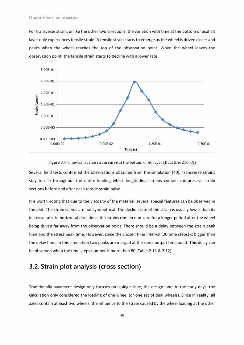
Chapter 3 Performance analysis
36
For transverse strain, unlike the other two directions, the variation with time at the bottom of asphalt
layer only experiences tensile strain. A tensile strain starts to emerge as the wheel is driven closer and
peaks when the wheel reaches the top of the observation point. When the wheel leaves the
observation point, the tensile strain starts to decline with a lower rate.
Figure 3.4 Time-transverse strain curve at the bottom of AC layer (Dual tire, 210 kN)
Several field tests confirmed the observations obtained from the simulation [40]. Transverse strains
stay tensile throughout the entire loading whilst longitudinal strains contain compressive strain
sections before and after each tensile strain pulse.
It is worth noting that due to the viscosity of the material, several special features can be observed in
the plot. The strain curves are not symmetrical. The decline rate of the strain is usually lower than its
increase rate. In horizontal directions, the strains remain non-zero for a longer period after the wheel
being driven far away from the observation point. There should be a delay between the strain peak
time and the stress peak time. However, since the chosen time interval (20 time steps) is bigger than
the delay time, in this simulation two peaks are merged at the same output time point. This delay can
be observed when the time steps number is more than 80 (Table 2.11 & 2.12).
3.2. Strain plot analysis (cross section)
Traditionally pavement design only focuses on a single lane, the design lane. In the early days, the
calculation only considered the loading of one wheel (or one set of dual wheels). Since in reality, all
axles contain at least two wheels, the influence to the strain caused by the wheel loading at the other
0.00E+00
5.00E-06
1.00E-05
1.50E-05
2.00E-05
2.50E-05
3.00E-05
0.00E+00 9.00E-02 1.80E-01 2.70E-01
Stra
in (μ
m/m
)
Time (s)
+01
+01
+01
+01
+01
+00
+00

3.2 Strain plot analysis (cross section)
37
end of the axle should be considered. Modern motorways always consist of more than one lane, thus
logically the strain condition of one lane will be influenced by the loading on other lanes. In some
severe cases, i.e. vehicles running shoulder by shoulder, the distance between two adjacent wheels of
two vehicles is even smaller than their own axle track. Hence this phenomenon is also worth
investigating especially to find out whether there will be any fluctuation in the new design. Three
comparison tests are conducted to investigate this problem. The first two use the original design,
whereas the third one uses the new design.
Figure 3.5 Horizontal strains under single axle load (Original design, Broadband, 80km/h, AC bottom)
The first plot shows the horizontal strain situation when only one single axle loads the heavy traffic
lane. It is clear in this plot that the strain distribution on the load bearing lane is symmetrical. The load
on the heavy traffic lane does produce an influence on its neighbour lane with a limited effect radius.
To be specific, the strain caused by the load on the heavy traffic lane has a noticeable influence at the
adjacent wheel position on the light traffic lane. However, this influence diminishes so rapidly with the
increase of the distance away from the loading position that at the middle of the un-trafficked lane it
has already dropped to less than 1% of the maximum strain value. As a result, the influence on the far
wheel of the axle on the un-trafficked lane caused by the heavy traffic on the right-hand lane is so
small that it can be considered negligible.
-8.28E-02
3.57E+013.57E+01
-1.43E-02
3.58E+01 3.58E+01
-2.00E-05
-1.00E-05
0.00E+00
1.00E-05
2.00E-05
3.00E-05
4.00E-05
0.00E+00 2.50E+03 5.00E+03 7.50E+03 1.00E+04 1.25E+04 1.50E+04
Hor
izon
tal s
trai
n (μ
m/m
)
Road width (mm)
Transverse strain Logitudinal strain
+01
+01
+01
+01
+00
+01
+01

Chapter 3 Performance analysis
38
Later simulation indicates that the strain caused by a standard passenger car is around 10% of the
strain caused by the maximum axle load of a truck which is used here. This means that for the
passenger car lane the horizontal strain at bottom of the AC layer caused by the truck running on the
adjacent lane may cause equal or even worse damage to the passenger car lane than the passenger
car itself.
Figure 3.6 Horizontal strains under double axle loads (Original design, Broadband, 80k/h, AC bottom)
The second plot confirms the conclusions obtained from the first test. In this test two single axle loads
are placed on both light and heavy traffic lanes. The strain values at the far end of the axle remains the
same as the values when only one axle loading is applied which proves that the influence caused by
the load on one lane to the far end of another lane is negligible. On contrast, the strain values at the
near end do experience variations. For the longitudinal strain there is an increase while for the
transverse train there is a decline. These variations are the result of the different influences caused by
the load on the other lanes. Although right under the centre of a wheel the horizontal strains in both
directions are tensile, the signs of their effective strains on the adjacent wheel are opposite to each
other. The first test has indicated that the loading on one lane will cause a tensile longitudinal strain
and a compressive transverse strain at the adjacent wheel position of the other lane.
2.98E+01 3.57E+01
3.91E+01 3.59E+01
-2.00E-05
-1.00E-05
0.00E+00
1.00E-05
2.00E-05
3.00E-05
4.00E-05
5.00E-05
0.00E+00 2.50E+03 5.00E+03 7.50E+03 1.00E+04 1.25E+04 1.50E+04
Hor
izon
tal s
trai
n (μ
m/m
)
Road width (mm)Transverse strain Logitudinal strain
+01
+01
+01
+01
+01
+00
+01
+01

3.2 Strain plot analysis (cross section)
39
Figure 3.7 Horizontal strains under double axle loads (New design, Broadband, 80km/h, AC bottom)
The third plot is used to compare with the second plot. The comparison indicates that with the new
design, the thickness reduction of the light traffic lane to be specific, does not lead to a negative
influence on the heavy traffic lane. Strain values of both near and far ends of the axle almost remain
the same comparing to the original design. Thus the new design is able to reduce the thickness of the
lighter traffic lanes without negatively effecting the performance of the heavy traffic lane whose
thickness remains the same.
The latter two plots illustrate that when two vehicles running shoulder by shoulder on two lanes, the
longitudinal strains at the near ends of the axles will increase while the transverse strains will decrease.
Hence it is suggested that for the fatigue evaluation the negative effect of longitudinal strain should
be noticed and discussed.
These tests also provide a possibility of simplifying the strain calculation procedure. Since the new
design hardly has any changes in strain condition of the heavy traffic lane, all the necessary data,
namely the horizontal strains at the bottom of certain layers and vertical strains at top of both reduced
and unchanged lanes, can be obtained from a single test on the new design instead of running two
tests on both original and new design models. By doing this the test time can be dramatically reduced.
Additionally, strain plots for different vehicle speeds are also proceeded. It can be easily observed that
vehicle with lower speed will produce larger strain response and lead to more severe damage to the
pavement structure.
2.97E+01 3.58E+01
3.91E+01 3.59E+01
-2.00E-05
-1.00E-05
0.00E+00
1.00E-05
2.00E-05
3.00E-05
4.00E-05
5.00E-05
0.00E+00 2.50E+03 5.00E+03 7.50E+03 1.00E+04 1.25E+04 1.50E+04
Hor
izon
tal s
trai
n (μ
m/m
)
Road width (mm)Transverse strain Logitudinal strain
+01
+01
+01
+01
+01
+00
+01
+01

Chapter 3 Performance analysis
40
Figure 3.8 Horizontal strains under double axle loads (New design, Broadband, 10km/h, AC bottom)
Figure 3.9 Maximum horizontal tensile strains at the bottom of AC layer under different vehicle speeds (Original design, Broadband)
Figure 3.9 indicates that as the vehicle speed decreases, both transverse and longitudinal strains
increase. The increase rates of the two directions are not the same therefore in this case at the lower
speed range the transverse strains become larger than longitudinal strains. Furthermore, the increase
rates also rise noticeably when the vehicle speed is lower than 40 km/h. Hence the traffic load with a
lower speed will cause more severe damages to the pavement. In practice traffic speed should be
maintained above a certain value.
4.48E+01
5.26E+015.24E+01
4.88E+01
-3.00E-05-2.00E-05-1.00E-050.00E+001.00E-052.00E-053.00E-054.00E-055.00E-056.00E-05
0.00E+00 2.50E+03 5.00E+03 7.50E+03 1.00E+04 1.25E+04 1.50E+04
Hor
izon
tal s
trai
n (μ
m/m
)
Road width (mm)
Transverse strain Logitudinal strain
3.00E-05
3.50E-05
4.00E-05
4.50E-05
5.00E-05
5.50E-05
6.00E-05
0 10 20 30 40 50 60 70 80 90
Hor
izon
tal s
trai
n (μ
m/m
)
Vehicle speed (km/h)Transverse starin Longitudinal strain
+01 +01 +01 +01 +01 +01 +00 +01 +01 +01
+01
+01
+01
+01
+01
+01
+01

3.3 Longitudinal strain versus Transverse strain
41
3.3. Longitudinal strain versus Transverse strain
In the Dutch design method, the rectangular tire prints are converted into equivalent circular prints
[23]. Plus the basic assumption that all the layers are homogenous, isotropic and horizontally infinite,
the horizontal strains calculated from the software are therefore also isotropic.
However in reality, although the shape of a tire print is not an ideal rectangle, it is far more different
from a circle [43]. As a result the longitudinal and transverse strain are hardly the same. Many field
tests have proved this difference. In a NCAT research, the strains of two orientations were investigated
to determine which, or both, should be considered in the fatigue prediction models [44]. To compare
the two responses, the maximum transverse reading was plotted against the maximum longitudinal
reading for each pass, shown in figure 3.10. There is quite a bit of scatter in the data since it was pooled
over a wide range of conditions, however, generally speaking the strain was higher in the longitudinal
direction rather than the transverse. Al-Qadi et al. also observed that the longitudinal strain was higher
than the complimentary transverse strain [45]. Some design methods suggest to consider the two
strains using an average value, though it can be clearly seen that an average value would falsely reduce
the strain value. In this NCAT research, it was decided to use the most severe response in its analysis.
To stay consistent throughout the procedure, only the longitudinal strain was considered in its
development of the fatigue functions in this NCAT research.
Figure 3.10 Transverse vs. Longitudinal Strain [44]
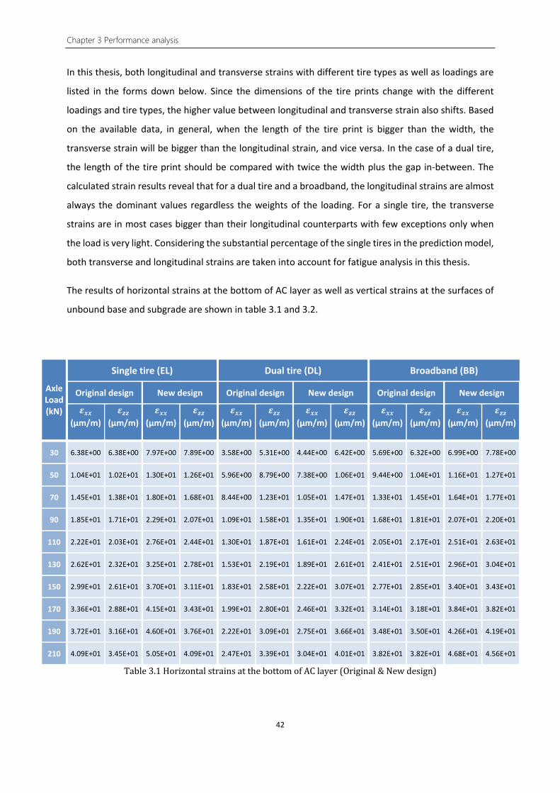
Chapter 3 Performance analysis
42
In this thesis, both longitudinal and transverse strains with different tire types as well as loadings are
listed in the forms down below. Since the dimensions of the tire prints change with the different
loadings and tire types, the higher value between longitudinal and transverse strain also shifts. Based
on the available data, in general, when the length of the tire print is bigger than the width, the
transverse strain will be bigger than the longitudinal strain, and vice versa. In the case of a dual tire,
the length of the tire print should be compared with twice the width plus the gap in-between. The
calculated strain results reveal that for a dual tire and a broadband, the longitudinal strains are almost
always the dominant values regardless the weights of the loading. For a single tire, the transverse
strains are in most cases bigger than their longitudinal counterparts with few exceptions only when
the load is very light. Considering the substantial percentage of the single tires in the prediction model,
both transverse and longitudinal strains are taken into account for fatigue analysis in this thesis.
The results of horizontal strains at the bottom of AC layer as well as vertical strains at the surfaces of
unbound base and subgrade are shown in table 3.1 and 3.2.
Axle Load (kN)
Single tire (EL) Dual tire (DL) Broadband (BB)
Original design New design Original design New design Original design New design
𝜺𝜺𝒙𝒙𝒙𝒙 (μm/m)
𝜺𝜺𝒛𝒛𝒛𝒛 (μm/m)
𝜺𝜺𝒙𝒙𝒙𝒙 (μm/m)
𝜺𝜺𝒛𝒛𝒛𝒛 (μm/m)
𝜺𝜺𝒙𝒙𝒙𝒙 (μm/m)
𝜺𝜺𝒛𝒛𝒛𝒛 (μm/m)
𝜺𝜺𝒙𝒙𝒙𝒙 (μm/m)
𝜺𝜺𝒛𝒛𝒛𝒛 (μm/m)
𝜺𝜺𝒙𝒙𝒙𝒙 (μm/m)
𝜺𝜺𝒛𝒛𝒛𝒛 (μm/m)
𝜺𝜺𝒙𝒙𝒙𝒙 (μm/m)
𝜺𝜺𝒛𝒛𝒛𝒛 (μm/m)
30 6.38E+00 6.38E+00 7.97E+00 7.89E+00 3.58E+00 5.31E+00 4.44E+00 6.42E+00 5.69E+00 6.32E+00 6.99E+00 7.78E+00
50 1.04E+01 1.02E+01 1.30E+01 1.26E+01 5.96E+00 8.79E+00 7.38E+00 1.06E+01 9.44E+00 1.04E+01 1.16E+01 1.27E+01
70 1.45E+01 1.38E+01 1.80E+01 1.68E+01 8.44E+00 1.23E+01 1.05E+01 1.47E+01 1.33E+01 1.45E+01 1.64E+01 1.77E+01
90 1.85E+01 1.71E+01 2.29E+01 2.07E+01 1.09E+01 1.58E+01 1.35E+01 1.90E+01 1.68E+01 1.81E+01 2.07E+01 2.20E+01
110 2.22E+01 2.03E+01 2.76E+01 2.44E+01 1.30E+01 1.87E+01 1.61E+01 2.24E+01 2.05E+01 2.17E+01 2.51E+01 2.63E+01
130 2.62E+01 2.32E+01 3.25E+01 2.78E+01 1.53E+01 2.19E+01 1.89E+01 2.61E+01 2.41E+01 2.51E+01 2.96E+01 3.04E+01
150 2.99E+01 2.61E+01 3.70E+01 3.11E+01 1.83E+01 2.58E+01 2.22E+01 3.07E+01 2.77E+01 2.85E+01 3.40E+01 3.43E+01
170 3.36E+01 2.88E+01 4.15E+01 3.43E+01 1.99E+01 2.80E+01 2.46E+01 3.32E+01 3.14E+01 3.18E+01 3.84E+01 3.82E+01
190 3.72E+01 3.16E+01 4.60E+01 3.76E+01 2.22E+01 3.09E+01 2.75E+01 3.66E+01 3.48E+01 3.50E+01 4.26E+01 4.19E+01
210 4.09E+01 3.45E+01 5.05E+01 4.09E+01 2.47E+01 3.39E+01 3.04E+01 4.01E+01 3.82E+01 3.82E+01 4.68E+01 4.56E+01
Table 3.1 Horizontal strains at the bottom of AC layer (Original & New design)

3.4 Pavement performance prediction
43
Axle Load (kN)
Single tire (EL) Dual tire (DL) Broadband (BB)
Original design New design Original design New design Original design New design
𝜺𝜺𝒃𝒃𝒃𝒃𝒃𝒃𝒃𝒃 (μm/m)
𝜺𝜺𝒃𝒃𝒔𝒔𝒃𝒃𝒔𝒔 (μm/m)
𝜺𝜺𝒃𝒃𝒃𝒃𝒃𝒃𝒃𝒃 (μm/m)
𝜺𝜺𝒃𝒃𝒔𝒔𝒃𝒃𝒔𝒔 (μm/m)
𝜺𝜺𝒃𝒃𝒃𝒃𝒃𝒃𝒃𝒃 (μm/m)
𝜺𝜺𝒃𝒃𝒔𝒔𝒃𝒃𝒔𝒔 (μm/m)
𝜺𝜺𝒃𝒃𝒃𝒃𝒃𝒃𝒃𝒃 (μm/m)
𝜺𝜺𝒃𝒃𝒔𝒔𝒃𝒃𝒔𝒔 (μm/m)
𝜺𝜺𝒃𝒃𝒃𝒃𝒃𝒃𝒃𝒃 (μm/m)
𝜺𝜺𝒃𝒃𝒔𝒔𝒃𝒃𝒔𝒔 (μm/m)
𝜺𝜺𝒃𝒃𝒃𝒃𝒃𝒃𝒃𝒃 (μm/m)
𝜺𝜺𝒃𝒃𝒔𝒔𝒃𝒃𝒔𝒔 (μm/m)
30 -1.94E+01 -3.44E+01 -2.37E+01 -3.86E+01 -1.52E+01 -3.27E+01 -1.81E+01 -3.62E+01 -1.87E+01 -3.44E+01 -3.85E+01 -3.85E+01
50 -3.17E+01 -5.69E+01 -3.85E+01 -6.39E+01 -2.52E+01 -5.44E+01 -3.00E+01 -6.03E+01 -3.10E+01 -5.73E+01 -3.74E+01 -6.41E+01
70 -4.37E+01 -7.95E+01 -5.30E+01 -8.93E+01 -3.55E+01 -7.67E+01 -4.22E+01 -8.51E+01 -4.37E+01 -8.13E+01 -5.26E+01 -9.08E+01
90 -5.54E+01 -1.02E+02 -6.71E+01 -1.15E+02 -4.60E+01 -9.98E+01 -5.46E+01 -1.11E+02 -5.50E+01 -1.03E+02 -6.62E+01 -1.15E+02
110 -6.67E+01 -1.24E+02 -8.06E+01 -1.39E+02 -5.48E+01 -1.19E+02 -6.50E+01 -1.32E+02 -6.67E+01 -1.26E+02 -8.02E+01 -1.40E+02
130 -7.80E+01 -1.47E+02 -9.41E+01 -1.65E+02 -6.45E+01 -1.41E+02 -7.64E+01 -1.56E+02 -7.82E+01 -1.48E+02 -9.40E+01 -1.66E+02
150 -8.89E+01 -1.69E+02 -1.07E+02 -1.90E+02 -7.64E+01 -1.66E+02 -9.02E+01 -1.84E+02 -8.96E+01 -1.71E+02 -1.08E+02 -1.91E+02
170 -9.96E+01 -1.91E+02 -1.20E+02 -2.14E+02 -8.35E+01 -1.84E+02 -9.87E+01 -2.04E+02 -1.01E+02 -1.94E+02 -1.21E+02 -2.17E+02
190 -1.10E+02 -2.13E+02 -1.33E+02 -2.39E+02 -9.29E+01 -2.06E+02 -1.10E+02 -2.28E+02 -1.12E+02 -2.16E+02 -1.34E+02 -2.42E+02
210 -1.21E+02 -2.35E+02 -1.46E+02 -2.63E+02 -1.03E+02 -2.28E+02 -1.21E+02 -2.53E+02 -1.23E+02 -2.38E+02 -1.47E+02 -2.66E+02
Table 3.2 Vertical strains at the surfaces of unbound base and subgrade (Original & New design)
3.4. Pavement performance prediction
The background report of OIA provides an outline of the Dutch design method. With the strain values
obtained from CAPA-3D, a series of performance predictions in the OIA software can be recreated
manually following the instructions.
3.4.1. Basic parameters
3.4.1.1. Traffic data
When evaluating the performance of the pavement it is assumed that each passage of a vehicle axle
will cause certain damage to the pavement structure. The number of the passing axles, the axle load
spectrum and the tire spectrum of the passing vehicles are the most important and fundamental
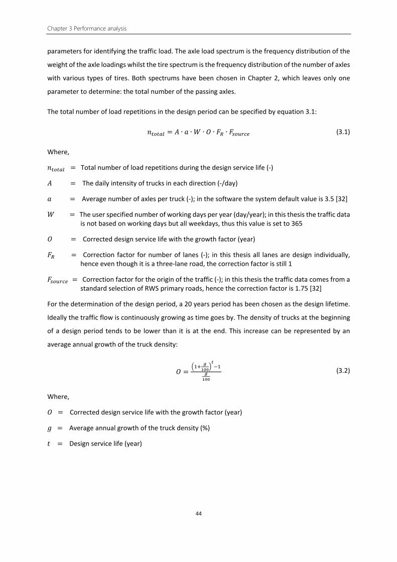
Chapter 3 Performance analysis
44
parameters for identifying the traffic load. The axle load spectrum is the frequency distribution of the
weight of the axle loadings whilst the tire spectrum is the frequency distribution of the number of axles
with various types of tires. Both spectrums have been chosen in Chapter 2, which leaves only one
parameter to determine: the total number of the passing axles.
The total number of load repetitions in the design period can be specified by equation 3.1:
𝑛𝑛𝑡𝑡𝑣𝑣𝑡𝑡𝑏𝑏𝑣𝑣 = 𝐴𝐴 ∙ 𝑎𝑎 ∙ 𝑊𝑊 ∙ 𝑂𝑂 ∙ 𝐹𝐹𝑅𝑅 ∙ 𝐹𝐹𝑠𝑠𝑣𝑣𝑠𝑠𝑛𝑛𝑠𝑠𝑑𝑑 (3.1)
Where,
𝑛𝑛𝑡𝑡𝑣𝑣𝑡𝑡𝑏𝑏𝑣𝑣 = Total number of load repetitions during the design service life (-)
𝐴𝐴 = The daily intensity of trucks in each direction (-/day)
𝑎𝑎 = Average number of axles per truck (-); in the software the system default value is 3.5 [32]
𝑊𝑊 = The user specified number of working days per year (day/year); in this thesis the traffic data is not based on working days but all weekdays, thus this value is set to 365
𝑂𝑂 = Corrected design service life with the growth factor (year)
𝐹𝐹𝑅𝑅 = Correction factor for number of lanes (-); in this thesis all lanes are design individually, hence even though it is a three-lane road, the correction factor is still 1
𝐹𝐹𝑠𝑠𝑣𝑣𝑠𝑠𝑛𝑛𝑠𝑠𝑑𝑑 = Correction factor for the origin of the traffic (-); in this thesis the traffic data comes from a standard selection of RWS primary roads, hence the correction factor is 1.75 [32]
For the determination of the design period, a 20 years period has been chosen as the design lifetime.
Ideally the traffic flow is continuously growing as time goes by. The density of trucks at the beginning
of a design period tends to be lower than it is at the end. This increase can be represented by an
average annual growth of the truck density:
𝑂𝑂 =�1+ 𝑔𝑔
100�𝑡𝑡−1
𝑔𝑔100
(3.2)
Where,
𝑂𝑂 = Corrected design service life with the growth factor (year)
𝑔𝑔 = Average annual growth of the truck density (%)
𝑡𝑡 = Design service life (year)

3.4 Pavement performance prediction
45
3.4.1.2. Adjustment for lateral wander
Trucks cannot, in practice, all move in the same perfect straight line on the road [46]. The position of
a wheel set shifts within a certain range along the transverse direction. This phenomenon is called
lateral wander. When considering the lateral wander, the vehicles are no longer driven on the same
track line, but in a certain bandwidth around the middle of the track line. The lateral wander can
dramatically affect the performance predictions of the designed pavement since the loadings are no
longer concentrated at the same position. Hence it is important to introduce a factor for lateral wander
in the design procedure.
Figure 3.11 Probability density and vertical strain distribution caused by a wheel [32]
The lateral wander factor mainly depends on lane width, vehicle width, vehicle speed and extent of
rutting. The distribution of the wheel position along the transverse direction is assumed to be a Laplace
distribution. The probability density function of the Laplace distribution is:
𝑓𝑓(𝑖𝑖) = 12𝜆𝜆∙ 𝑒𝑒−
|𝑥𝑥−𝜇𝜇|𝜆𝜆 (3.3)
Where,
𝑓𝑓(𝑖𝑖) = Probability density (%/cm)
Strip width
Track line
Vertical Strain (m/m)
Probability density (%/cm)
Distance (cm) 0
Vertical strain at the bottom of asphalt layer
Probability of distance 𝒙𝒙

Chapter 3 Performance analysis
46
𝑥𝑥 = Distance from the centre of the track line (cm)
𝜇𝜇 = Average value (cm)
𝜆𝜆 = Scale parameter (cm)
For the lateral wander factor, the centre of the track line is taken as the reference point. The value of
μ is therefore 0. The scale parameter indicates the shape of the distribution curve. A small value
indicated a narrow distribution which means a limited lateral wander range.
Equation 3.4 shows the relationship between scale parameter and standard deviation.
𝜆𝜆 = 𝜎𝜎√2 (3.4)
Where,
𝜆𝜆 = Scale parameter (cm)
𝜎𝜎 = Standard deviation (cm)
The standard deviation of the lateral wander is described by the following settings:
𝜎𝜎𝑏𝑏 = 𝑏𝑏0 + 𝑏𝑏1 ∙ 𝑅𝑅𝑑𝑑𝑑𝑑𝑒𝑒𝑑𝑑 (3.5)
Where,
𝜎𝜎𝑏𝑏 = Standard deviation of lateral wander (cm)
𝑏𝑏0 , 𝑏𝑏1 = Model coefficients based on tire types, allowed maximum rutting depth and vehicle speed (cm)
𝑅𝑅𝑑𝑑𝑑𝑑𝑒𝑒𝑑𝑑 = Edge width class, varies from 1 to 6 (-)
The edge width is defined as the distance between the tire print edge and the edge of the lane. The
determination of the edge width class is dependent on the lane width, the truck width as well as the
truck type. Light trucks have smaller width with an average from 2.00 m to 2.25 m while heavy trucks
have an average width between 2.25 m to 2.50 m [32]. In this thesis the truck width (distance between
tires outside edges) is set to a fixed value of 2.30 m. The edge width class can be obtained by the
following formula:
𝑅𝑅𝑑𝑑𝑑𝑑𝑒𝑒𝑑𝑑 = (𝑏𝑏𝑣𝑣𝑏𝑏𝑏𝑏𝑑𝑑 − 2.75)0.25� (3.6)
Where,
𝑅𝑅𝑑𝑑𝑑𝑑𝑒𝑒𝑑𝑑 = Edge width class, varies from 1 to 6 (-)
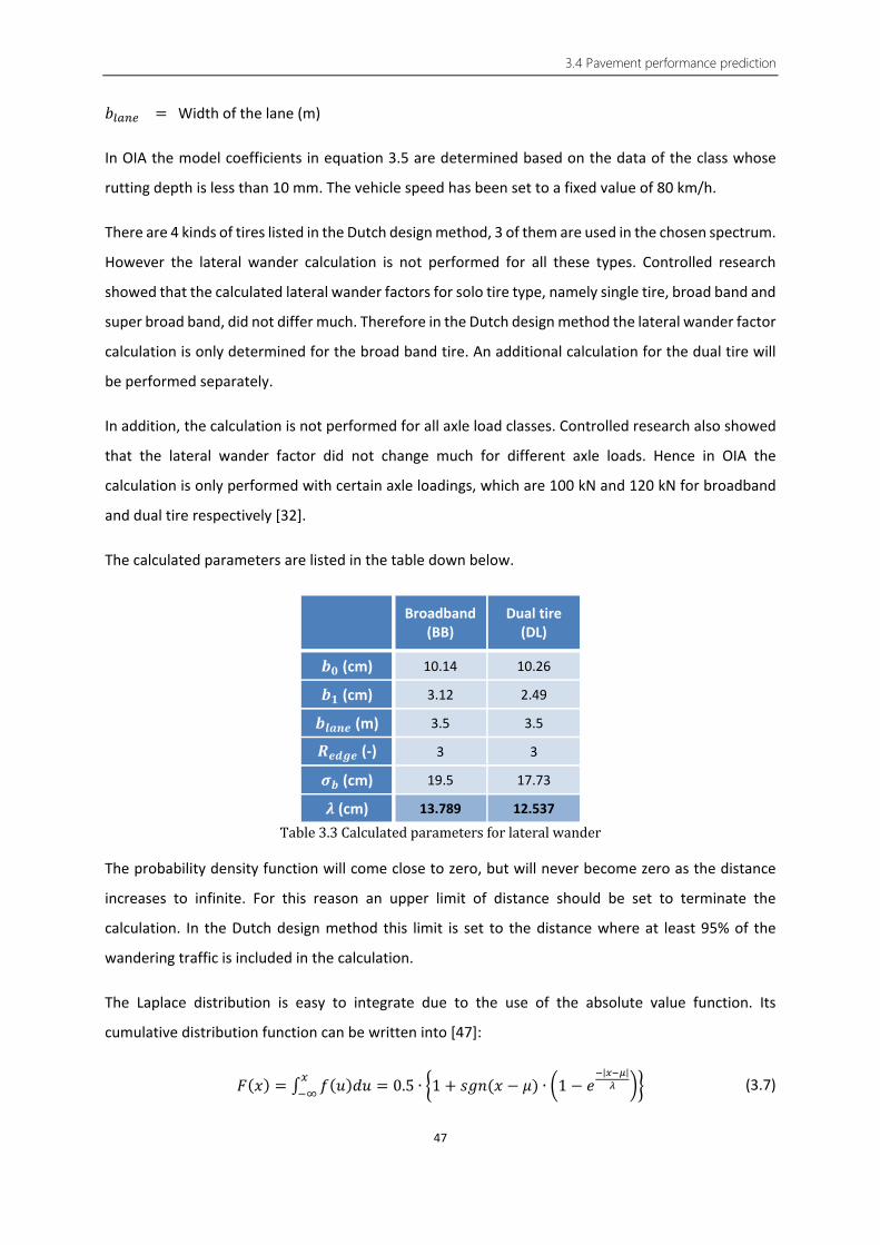
3.4 Pavement performance prediction
47
𝑏𝑏𝑣𝑣𝑏𝑏𝑏𝑏𝑑𝑑 = Width of the lane (m)
In OIA the model coefficients in equation 3.5 are determined based on the data of the class whose
rutting depth is less than 10 mm. The vehicle speed has been set to a fixed value of 80 km/h.
There are 4 kinds of tires listed in the Dutch design method, 3 of them are used in the chosen spectrum.
However the lateral wander calculation is not performed for all these types. Controlled research
showed that the calculated lateral wander factors for solo tire type, namely single tire, broad band and
super broad band, did not differ much. Therefore in the Dutch design method the lateral wander factor
calculation is only determined for the broad band tire. An additional calculation for the dual tire will
be performed separately.
In addition, the calculation is not performed for all axle load classes. Controlled research also showed
that the lateral wander factor did not change much for different axle loads. Hence in OIA the
calculation is only performed with certain axle loadings, which are 100 kN and 120 kN for broadband
and dual tire respectively [32].
The calculated parameters are listed in the table down below.
Broadband (BB)
Dual tire (DL)
𝒃𝒃𝟎𝟎 (cm) 10.14 10.26
𝒃𝒃𝟏𝟏 (cm) 3.12 2.49
𝒃𝒃𝒍𝒍𝒃𝒃𝒍𝒍𝒃𝒃 (m) 3.5 3.5
𝑹𝑹𝒃𝒃𝒆𝒆𝒔𝒔𝒃𝒃 (-) 3 3
𝝈𝝈𝒃𝒃 (cm) 19.5 17.73
𝝀𝝀 (cm) 13.789 12.537
Table 3.3 Calculated parameters for lateral wander
The probability density function will come close to zero, but will never become zero as the distance
increases to infinite. For this reason an upper limit of distance should be set to terminate the
calculation. In the Dutch design method this limit is set to the distance where at least 95% of the
wandering traffic is included in the calculation.
The Laplace distribution is easy to integrate due to the use of the absolute value function. Its
cumulative distribution function can be written into [47]:
𝐹𝐹(𝑥𝑥) = ∫ 𝑓𝑓(𝑢𝑢)𝑑𝑑𝑢𝑢 = 0.5 ∙ �1 + 𝑠𝑠𝑔𝑔𝑛𝑛(𝑥𝑥 − 𝜇𝜇) ∙ �1 − 𝑒𝑒−|𝑥𝑥−𝜇𝜇|
𝜆𝜆 ��𝑎𝑎−∞ (3.7)

Chapter 3 Performance analysis
48
Notice that the cumulative distribution function gives the output between negative infinity to the
target distance. For lateral wander the wheel is assumed to be driven in a symmetrical area with a
centre track line. Hence the lateral wander distribution area should be determined with an additional
step:
𝐹𝐹(𝑥𝑥)′ = ∫ 𝑓𝑓(𝑢𝑢)𝑑𝑑𝑢𝑢 = 2 ∙ [𝐹𝐹(𝑥𝑥) − 0.5]𝑎𝑎−𝑎𝑎
= 2𝐹𝐹(𝑥𝑥) − 1 (3.8)
Where,
𝐹𝐹(𝑥𝑥) = Cumulative probability from distance −∞ to 𝑥𝑥 (%)
𝐹𝐹(𝑥𝑥)′ = Cumulative probability from distance −𝑥𝑥 to 𝑥𝑥 (%)
𝑓𝑓(𝑢𝑢) = Probability density at 𝑢𝑢 (-)
𝑥𝑥 = Distance from the centre of the track line (m)
𝜇𝜇 = Average value (m)
𝜆𝜆 = Scale parameter (-)
The lateral wander areas for both broadband and dual tire are listed in table 3.4:
Broadband (BB) Dual tire (DL)
𝒙𝒙 (cm) 𝑭𝑭(𝒙𝒙) 𝑭𝑭(𝒙𝒙)′ 𝒙𝒙 (cm) 𝑭𝑭(𝒙𝒙) 𝑭𝑭(𝒙𝒙)′
0 50.00% 0.00% 0 50.00% 0.00%
2.5 58.29% 16.58% 2.5 59.04% 18.08%
7.5 70.98% 41.95% 7.5 72.51% 45.02%
12.5 79.80% 59.61% 12.5 81.55% 63.10%
17.5 85.95% 71.89% 17.5 87.62% 75.24%
22.5 90.22% 80.44% 22.5 91.69% 83.38%
27.5 93.20% 86.39% 27.5 94.42% 88.85%
32.5 95.26% 90.53% 32.5 96.26% 92.52%
37.5 96.71% 93.41% 37.5 97.49% 94.98%
42.5 97.71% 95.41% 42.5 98.31% 96.63%
Table 3.4 Lateral wander area for broadband and dual tire
Once the lateral wander area is determined, it will be divided into several strips with a certain width
to continue the calculation of the correction factor for lateral wander. Due to the dimension design of
the mesh, the strip width is fixed to 5 cm as shown in table 3.4. For each strip the allowable number of

3.4 Pavement performance prediction
49
load repetitions is determined. The formulas used here are same as the ones calculating the allowable
number of load repetitions of different construction layers on the basis of the horizontal strain or
vertical deformation at the certain position. To determine the lateral wander factor, firstly the damage
factor when all traffic is driven right on the track line is calculated by equation 3.9:
𝐷𝐷0 = 1𝑁𝑁(0) (3.9)
Where,
𝐷𝐷0 = Damage factor when 100% of the traffic runs right on the track line (-)
𝑁𝑁(0) = Permissible number of load repetitions (-)
Then the damage factor when lateral wander occurs is also determined. The damage factors of all
strips are calculated separately and summed up by equation 3.10:
𝐷𝐷𝑉𝑉 =𝑓𝑓[0]𝑁𝑁[0] + 2 ∙ �
𝑓𝑓[𝑖𝑖]𝑁𝑁[𝑖𝑖]
𝑏𝑏𝑠𝑠𝑡𝑡𝑛𝑛𝑠𝑠𝑠𝑠−1
𝑖𝑖=1
(3.10)
Where,
𝐷𝐷𝑉𝑉 = Summed damage factor of all strips (-)
𝑓𝑓[0] = Percentage of traffic runs right on the central strip (%)
𝑁𝑁[0] = Permissible number of load repetitions on the central strip (-)
𝑛𝑛𝑠𝑠𝑡𝑡𝑛𝑛𝑖𝑖𝑠𝑠 = Number of strips (-)
𝑓𝑓[𝑖𝑖] = Percentage of traffic runs on strip 𝑖𝑖 (%)
𝑁𝑁[𝑖𝑖] = Permissible number if load repetitions on strip 𝑖𝑖 (-)
After obtaining the damage factors under two different circumstances, the final lateral wander factor
can be easy determined by equation 3.11:
𝐹𝐹𝑆𝑆 = 𝐷𝐷𝑉𝑉𝐷𝐷0
(3.11)
Where,
𝐹𝐹𝑆𝑆 = Correction factor for lateral wander (-)
𝐷𝐷𝑉𝑉 = Summed damage factor when lateral wander occurs (-)
𝐷𝐷0 = Damage factor when all traffic is driven right on the track line (-)
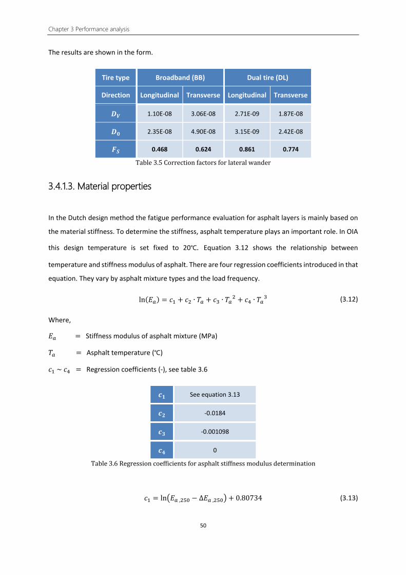
Chapter 3 Performance analysis
50
The results are shown in the form.
Tire type Broadband (BB) Dual tire (DL)
Direction Longitudinal Transverse Longitudinal Transverse
𝑫𝑫𝑽𝑽 1.10E-08 3.06E-08 2.71E-09 1.87E-08
𝑫𝑫𝟎𝟎 2.35E-08 4.90E-08 3.15E-09 2.42E-08
𝑭𝑭𝑺𝑺 0.468 0.624 0.861 0.774
Table 3.5 Correction factors for lateral wander
3.4.1.3. Material properties
In the Dutch design method the fatigue performance evaluation for asphalt layers is mainly based on
the material stiffness. To determine the stiffness, asphalt temperature plays an important role. In OIA
this design temperature is set fixed to 20℃. Equation 3.12 shows the relationship between
temperature and stiffness modulus of asphalt. There are four regression coefficients introduced in that
equation. They vary by asphalt mixture types and the load frequency.
ln(𝜏𝜏𝑏𝑏) = 𝑐𝑐1 + 𝑐𝑐2 ∙ 𝑇𝑇𝑏𝑏 + 𝑐𝑐3 ∙ 𝑇𝑇𝑏𝑏2 + 𝑐𝑐4 ∙ 𝑇𝑇𝑏𝑏3 (3.12)
Where,
𝜏𝜏𝑏𝑏 = Stiffness modulus of asphalt mixture (MPa)
𝑇𝑇𝑏𝑏 = Asphalt temperature (℃)
𝑐𝑐1 ~ 𝑐𝑐4 = Regression coefficients (-), see table 3.6
𝒄𝒄𝟏𝟏 See equation 3.13
𝒄𝒄𝟐𝟐 -0.0184
𝒄𝒄𝟑𝟑 -0.001098
𝒄𝒄𝟒𝟒 0
Table 3.6 Regression coefficients for asphalt stiffness modulus determination
𝑐𝑐1 = ln�𝜏𝜏𝑏𝑏 ,250 − Δ𝜏𝜏𝑏𝑏 ,250� + 0.80734 (3.13)
3.4 Pavement performance prediction
51
Where,
𝜏𝜏𝑏𝑏 ,250 = Stiffness modulus of asphalt according to test 62 of the Standard RAW Provision 2010 (MPa)
Δ𝜏𝜏𝑏𝑏 ,250 = Stiffness reduction depending on the test load distribution and repetition number of the
tests (MPa), in this thesis the stiffness reduction is set to 1285 MPa [32]
In test 62 of the Standard RAW Provision 2010, the stiffness modulus of asphalt material is only
required at a single temperature (20℃) and load frequency (8 Hz) [32]. In practice there are obviously
various vehicle speeds. A different load speed can be converted to an equivalent load frequency and
then to a fictive temperature, which is used in equation 3.12 to calculate the stiffness modulus.
𝑇𝑇𝑓𝑓𝑖𝑖𝑠𝑠𝑡𝑡 = 1
1𝑇𝑇𝑏𝑏+273
−log �𝑓𝑓𝑡𝑡𝑡𝑡𝑠𝑠𝑡𝑡𝑓𝑓 �
𝐶𝐶
− 273 (3.14)
Where,
𝑇𝑇𝑓𝑓𝑖𝑖𝑠𝑠𝑡𝑡 = Fictive temperature for the determination of the asphalt stiffness (℃)
𝑇𝑇𝑏𝑏 = Design temperature (℃), 20 ℃ in this case
𝑓𝑓𝑡𝑡𝑑𝑑𝑠𝑠𝑡𝑡 = Load frequency used in the standard test (Hz), 8 Hz in this case
𝑓𝑓 = Load frequency of the design traffic speed (HZ);
𝐶𝐶 = Experimentally determined constant (K), 11242 K in this case [32]
The traffic speed can be converted into the frequency of a sinusoidal load by equation 3.15:
log�𝑓𝑓𝑑𝑑𝑒𝑒� = −0.6 − 0.5 ∙ ℎ𝑏𝑏 + 0.94 ∙ log (𝑉𝑉) (3.15)
Where,
𝑓𝑓𝑑𝑑𝑒𝑒 = Equivalent load frequency of the design traffic speed (Hz)
ℎ𝑏𝑏 = Asphalt layer thickness (m)
𝑉𝑉 = Design traffic speed (km/h)
In conclusion, the effect of a moving load at a certain speed is firstly converted into a load frequency.
Then on the basis of the master curve a corresponding fictive temperature of asphalt can be obtained.
With these parameters the stiffness modulus of the asphalt can be finally determined by the equation
3.12.
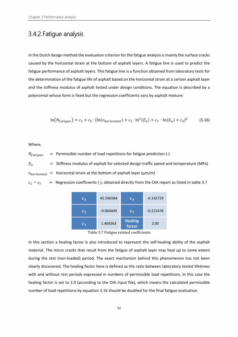
Chapter 3 Performance analysis
52
3.4.2. Fatigue analysis
In the Dutch design method the evaluation criterion for the fatigue analysis is mainly the surface cracks
caused by the horizontal strain at the bottom of asphalt layers. A fatigue line is used to predict the
fatigue performance of asphalt layers. This fatigue line is a function obtained from laboratory tests for
the determination of the fatigue life of asphalt based on the horizontal strain at a certain asphalt layer
and the stiffness modulus of asphalt tested under design conditions. The equation is described by a
polynomial whose form is fixed but the regression coefficients vary by asphalt mixture:
ln�𝑁𝑁𝑓𝑓𝑏𝑏𝑡𝑡𝑖𝑖𝑒𝑒𝑠𝑠𝑑𝑑� = 𝑐𝑐1 + 𝑐𝑐5 ∙ {ln(𝜀𝜀ℎ𝑣𝑣𝑛𝑛𝑖𝑖𝑜𝑜𝑣𝑣𝑏𝑏𝑡𝑡𝑏𝑏𝑣𝑣) + 𝑐𝑐2 ∙ ln2(𝜏𝜏𝑏𝑏) + 𝑐𝑐3 ∙ ln(𝜏𝜏𝑏𝑏) + 𝑐𝑐4}2 (3.16)
Where,
𝑁𝑁𝑓𝑓𝑏𝑏𝑡𝑡𝑖𝑖𝑒𝑒𝑠𝑠𝑑𝑑 = Permissible number of load repetitions for fatigue prediction (-)
𝜏𝜏𝑏𝑏 = Stiffness modulus of asphalt for selected design traffic speed and temperature (MPa)
𝜀𝜀ℎ𝑣𝑣𝑛𝑛𝑖𝑖𝑜𝑜𝑣𝑣𝑏𝑏𝑡𝑡𝑏𝑏𝑣𝑣 = Horizontal strain at the bottom of asphalt layer (μm/m)
𝑐𝑐1 ~ 𝑐𝑐5 = Regression coefficients (-), obtained directly from the OIA report as listed in table 3.7
𝒄𝒄𝟏𝟏 45.596584 𝒄𝒄𝟒𝟒 -0.142729
𝒄𝒄𝟐𝟐 -0.064449 𝒄𝒄𝟓𝟓 -0.222478
𝒄𝒄𝟑𝟑 1.404363 Healing factor
2.00
Table 3.7 Fatigue related coefficients
In this section a healing factor is also introduced to represent the self-healing ability of the asphalt
material. The micro cracks that result from the fatigue of asphalt layer may heal up to some extent
during the rest (non-loaded) period. The exact mechanism behind this phenomenon has not been
clearly discovered. The healing factor here is defined as the ratio between laboratory tested lifetimes
with and without rest periods expressed in numbers of permissible load repetitions. In this case the
healing factor is set to 2.0 (according to the OIA input file), which means the calculated permissible
number of load repetitions by equation 3.16 should be doubled for the final fatigue evaluation.

3.4 Pavement performance prediction
53
3.4.3. Permanent deformation analysis
In the Dutch design method the deformation at the surface of the unbound layers is considered as the
primary reason for the permanent deformation of a pavement. A relationship between unbound layer
deformation and vertical strain at the top of the layer has been determined. This relationship is
converted into a function and displayed down below:
log�𝑁𝑁𝑑𝑑𝑑𝑑𝑓𝑓𝑣𝑣𝑛𝑛𝑛𝑛� = 𝑐𝑐1 + 𝑐𝑐2 ∙ log (𝜀𝜀𝑣𝑣𝑑𝑑𝑛𝑛𝑡𝑡𝑖𝑖𝑠𝑠𝑏𝑏𝑣𝑣) (3.17)
Where,
𝑁𝑁𝑑𝑑𝑑𝑑𝑓𝑓𝑣𝑣𝑛𝑛𝑛𝑛 = Permissible number of load repetitions for permanent deformation prediction (-)
𝜀𝜀𝑣𝑣𝑑𝑑𝑛𝑛𝑡𝑡𝑖𝑖𝑠𝑠𝑏𝑏𝑣𝑣 = Vertical strain at the top of the targeted unbound layer (μm/m)
𝑐𝑐1 & 𝑐𝑐2 = Regression coefficients (-), 𝑐𝑐1 = 17.289 , 𝑐𝑐2 = −4.00
3.4.4. Performance prediction results
Following the fatigue and permanent deformation analysis procedure discussed in the former chapters,
the allowable numbers of load repetitions can be determined under all different load conditions and
tire prints. Then the ratio of fatigue or permanent deformation resistance of each axle load and tire
type combination is calculated. This rate is defined as the predicted number of axle passes of a certain
axle load and tire type divided by the allowed number of load repetitions for the pavement under the
same combination. Finally sum the ratios of fatigue or permanent deformation resistance of all the
combinations, considering several correction factors such as lateral wander, to evaluate the
performance of the designed pavement structure. This summation can be expressed as equation 3.18:
��𝑛𝑛𝑖𝑖𝑖𝑖𝑁𝑁𝑖𝑖𝑖𝑖
= 𝑀𝑀𝑡𝑡
𝑁𝑁𝑁𝑁
𝑁𝑁𝑁𝑁
𝑁𝑁𝑁𝑁
𝑁𝑁𝑁𝑁
(3.18)
Where,
𝑛𝑛𝑖𝑖𝑖𝑖 = Design number of load repetitions of axle load class 𝑖𝑖 and tire type 𝑗𝑗 (-)
𝑁𝑁𝑖𝑖𝑖𝑖 = Fatigue or permanent deformation resistance (allowed number of load repetitions) of axle load class 𝑖𝑖 and tire type 𝑗𝑗 (-)

Chapter 3 Performance analysis
54
𝑁𝑁𝑁𝑁 = Number of axle load classes (-)
𝑁𝑁𝑇𝑇 = Number of tire types (-)
𝑀𝑀𝑡𝑡 = Damage fraction (Miner’s rule) (-)
Here the Miner’s rule is used to evaluate the pavement performance. The relationship between
structural damage and the Miner number is listed in table 3.7 [23].
Structural damage
Strength fatigue
Miner number
5% 32% 0.32
10% 43% 0.43
15% 54% 0.54
20% 64% 0.64
25% 74% 0.74
Table 3.8 Relationship between asphalt structural damage and Miner number
Rijkswaterstaat stipulates a maximum permissible structural damage ratio of 15% for fatigue
evaluation, whose Miner number is 0.54 according to the table. For the permanent deformation
evaluation the maximum permissible Miner number is equal to 1. Therefore when the calculated Miner
number for fatigue is larger than 0.54 or for permanent deformation larger than 1, the designed
pavement structure will be considered to have failed and need to be re-designed.
Performance Miner number
AC layer fatigue 0.54
Unbound base deformation - (≈0)
Subgrade deformation 0.08
Table 3.9 Performance prediction by OIA (Miner number)
The calculated results for both original and new designs are listed in the table 3.10 and 3.11. For lane
3 the values remain the same since the thickness design of lane 3 remains the same.
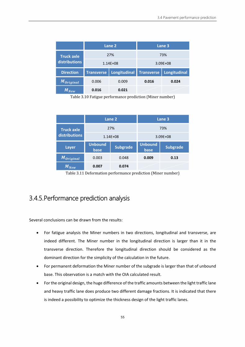
3.4 Pavement performance prediction
55
Lane 2 Lane 3
Truck axle distributions
27% 73%
1.14E+08 3.09E+08
Direction Transverse Longitudinal Transverse Longitudinal
𝑴𝑴𝑶𝑶𝑶𝑶𝒊𝒊𝒔𝒔𝒊𝒊𝒍𝒍𝒃𝒃𝒍𝒍 0.006 0.009 0.016 0.024
𝑴𝑴𝑵𝑵𝒃𝒃𝑵𝑵 0.016 0.021
Table 3.10 Fatigue performance prediction (Miner number)
Lane 2 Lane 3
Truck axle distributions
27% 73%
1.14E+08 3.09E+08
Layer Unbound base Subgrade Unbound
base Subgrade
𝑴𝑴𝑶𝑶𝑶𝑶𝒊𝒊𝒔𝒔𝒊𝒊𝒍𝒍𝒃𝒃𝒍𝒍 0.003 0.048 0.009 0.13
𝑴𝑴𝑵𝑵𝒃𝒃𝑵𝑵 0.007 0.074
Table 3.11 Deformation performance prediction (Miner number)
3.4.5. Performance prediction analysis
Several conclusions can be drawn from the results:
• For fatigue analysis the Miner numbers in two directions, longitudinal and transverse, are
indeed different. The Miner number in the longitudinal direction is larger than it in the
transverse direction. Therefore the longitudinal direction should be considered as the
dominant direction for the simplicity of the calculation in the future.
• For permanent deformation the Miner number of the subgrade is larger than that of unbound
base. This observation is a match with the OIA calculated result.
• For the original design, the huge difference of the traffic amounts between the light traffic lane
and heavy traffic lane does produce two different damage fractions. It is indicated that there
is indeed a possibility to optimize the thickness design of the light traffic lanes.
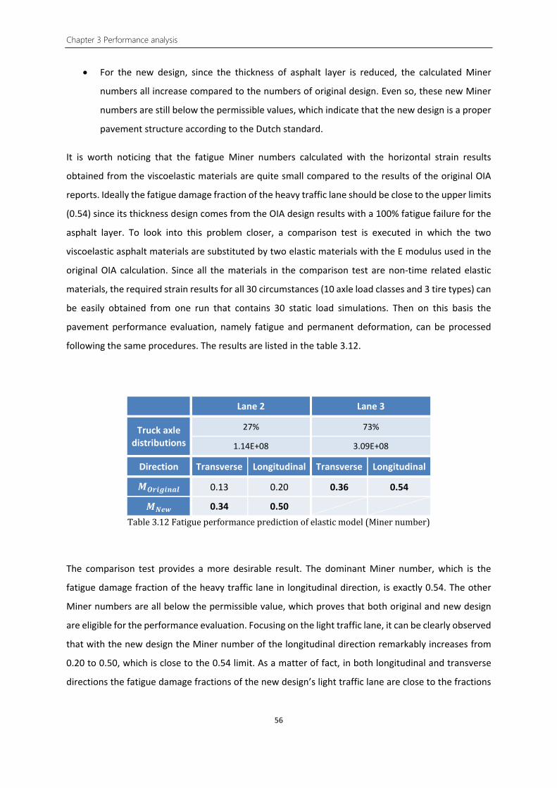
Chapter 3 Performance analysis
56
• For the new design, since the thickness of asphalt layer is reduced, the calculated Miner
numbers all increase compared to the numbers of original design. Even so, these new Miner
numbers are still below the permissible values, which indicate that the new design is a proper
pavement structure according to the Dutch standard.
It is worth noticing that the fatigue Miner numbers calculated with the horizontal strain results
obtained from the viscoelastic materials are quite small compared to the results of the original OIA
reports. Ideally the fatigue damage fraction of the heavy traffic lane should be close to the upper limits
(0.54) since its thickness design comes from the OIA design results with a 100% fatigue failure for the
asphalt layer. To look into this problem closer, a comparison test is executed in which the two
viscoelastic asphalt materials are substituted by two elastic materials with the E modulus used in the
original OIA calculation. Since all the materials in the comparison test are non-time related elastic
materials, the required strain results for all 30 circumstances (10 axle load classes and 3 tire types) can
be easily obtained from one run that contains 30 static load simulations. Then on this basis the
pavement performance evaluation, namely fatigue and permanent deformation, can be processed
following the same procedures. The results are listed in the table 3.12.
Lane 2 Lane 3
Truck axle distributions
27% 73%
1.14E+08 3.09E+08
Direction Transverse Longitudinal Transverse Longitudinal
𝑴𝑴𝑶𝑶𝑶𝑶𝒊𝒊𝒔𝒔𝒊𝒊𝒍𝒍𝒃𝒃𝒍𝒍 0.13 0.20 0.36 0.54
𝑴𝑴𝑵𝑵𝒃𝒃𝑵𝑵 0.34 0.50 Table 3.12 Fatigue performance prediction of elastic model (Miner number)
The comparison test provides a more desirable result. The dominant Miner number, which is the
fatigue damage fraction of the heavy traffic lane in longitudinal direction, is exactly 0.54. The other
Miner numbers are all below the permissible value, which proves that both original and new design
are eligible for the performance evaluation. Focusing on the light traffic lane, it can be clearly observed
that with the new design the Miner number of the longitudinal direction remarkably increases from
0.20 to 0.50, which is close to the 0.54 limit. As a matter of fact, in both longitudinal and transverse
directions the fatigue damage fractions of the new design’s light traffic lane are close to the fractions

3.4 Pavement performance prediction
57
of heavy traffic lane. This result is very meaningful since it shows that the new design causes the light
and heavy traffic lane to have a similar material utilization.
The comparison test indicates that the finite element model is able to provide proper results for the
pavement design. The small strain value issue is mainly because of the use of the viscoelastic material.
In general, the strain responses calculated from the viscoelastic model is around 50% of the strain
values calculated from the elastic model. After the Miner number calculation the difference becomes
even bigger.
Numerically it can be explained. The creep test for the AC material shows that within the short loading
time used in the moving load simulation the stiffness of the AC can be still very high compared to the
10000 MPa value used in the elastic simulation, which will lead to smaller strain responses.
Chapter 4 Long-term run analysis
58
4. Long-term run analysis
As discussed in the earlier chapters, although the finite element software is capable of calculating the
strain response of a pavement structure in a more direct way, the evaluation for the performance is
still on the basis of a series of empirical equations. Fortunately the finite element software is also able
to carry out a long-term simulation. With the introduction of the viscoelasticity or damage factor of a
material, the software can predict the pavement’s condition after thousands even millions of axle loads
passing by. It provides another perspective to evaluate the performance of pavement structures.
4.1. Real-life simulation
In most studies, there are mainly two ways of realizing a real-life simulation. The first one is converting
the moving load into a sinusoidal load applying at one position [48] whilst the second is to calculate
the accumulated impact time and punish the model with the same amount of time and load [49].
However, in reality a moving load almost never acts like a sinusoidal load or occurs at constant time
intervals. The various dimensions and distances between vehicles result in different strain peaks and
recovering time for each axle loads. Although it is definitely impossible to recreate the actual situation
on a pavement, there are still some efforts to be made to obtain a more suitable simulation.
4.1.1. Traffic load input
Traffic never distributes evenly during the 24 hours of a day or the 4 seasons of a year. The traffic
conditions, namely amount, loading classes or even speed, can be quite different between the rush
hours and the off-peak hours [50]. For example, during the rush hours the traffic amount will definitely
boost. As a result the time interval between vehicles will decline and lead to a shorter recovery time
for the pavement. However, in some statistical researches during the rush hours, the amount of heavy
trucks tends to decrease since they prefer to run during the off-peak hours [50]. Obviously it is neither
possible nor economical to make a 100% real simulation. Therefore a smart choice of traffic load input
is necessary.
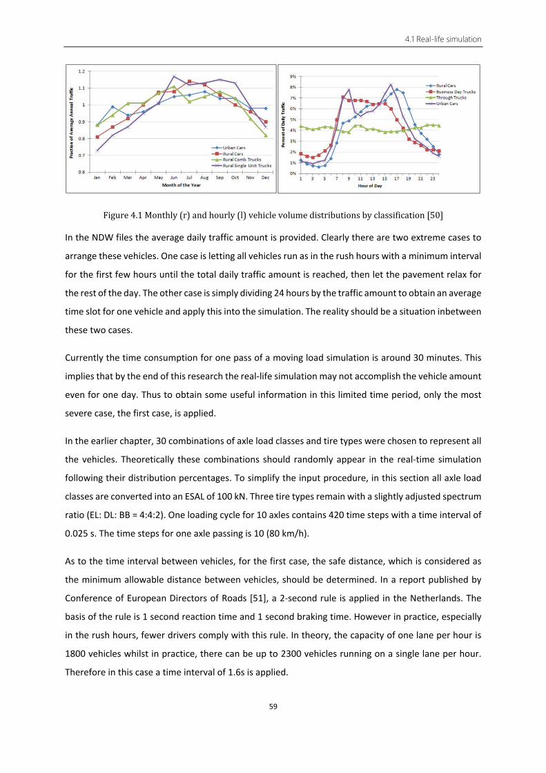
4.1 Real-life simulation
59
Figure 4.1 Monthly (r) and hourly (l) vehicle volume distributions by classification [50]
In the NDW files the average daily traffic amount is provided. Clearly there are two extreme cases to
arrange these vehicles. One case is letting all vehicles run as in the rush hours with a minimum interval
for the first few hours until the total daily traffic amount is reached, then let the pavement relax for
the rest of the day. The other case is simply dividing 24 hours by the traffic amount to obtain an average
time slot for one vehicle and apply this into the simulation. The reality should be a situation inbetween
these two cases.
Currently the time consumption for one pass of a moving load simulation is around 30 minutes. This
implies that by the end of this research the real-life simulation may not accomplish the vehicle amount
even for one day. Thus to obtain some useful information in this limited time period, only the most
severe case, the first case, is applied.
In the earlier chapter, 30 combinations of axle load classes and tire types were chosen to represent all
the vehicles. Theoretically these combinations should randomly appear in the real-time simulation
following their distribution percentages. To simplify the input procedure, in this section all axle load
classes are converted into an ESAL of 100 kN. Three tire types remain with a slightly adjusted spectrum
ratio (EL: DL: BB = 4:4:2). One loading cycle for 10 axles contains 420 time steps with a time interval of
0.025 s. The time steps for one axle passing is 10 (80 km/h).
As to the time interval between vehicles, for the first case, the safe distance, which is considered as
the minimum allowable distance between vehicles, should be determined. In a report published by
Conference of European Directors of Roads [51], a 2-second rule is applied in the Netherlands. The
basis of the rule is 1 second reaction time and 1 second braking time. However in practice, especially
in the rush hours, fewer drivers comply with this rule. In theory, the capacity of one lane per hour is
1800 vehicles whilst in practice, there can be up to 2300 vehicles running on a single lane per hour.
Therefore in this case a time interval of 1.6s is applied.

Chapter 4 Long-term run analysis
60
A standard two-axle truck with a front and rear wheelbase of 6.6m is chosen for the simulation [34].
Considering the tire length, the time for one truck passing by is 0.5s. Since in reality most of the front
axles are equipped with single tire, an order for the three tires’ appearance is settled.
Figure 4.2 Typical two-axle truck (VOLVO FL) [65]
To simulate the passing lane’s influence to the light traffic lane, a series of passenger cars are assigned
onto the passing lane. A 2-axle single-wheel passenger car with a wheelbase of 2.5 m and axle load of
7.5 kN is chosen as the representative model. The speed of passenger cars is set to 120 km/h with the
same 1.6 s following distance as trucks’. One loading cycle for each passenger car (2 axles) passing by
contains 67 time steps with the same time interval of 0.025 s. The time steps for one axle passing is 7
(120 km/h). The final traffic input is listed in table 4.1.
Lane 1 Passenger cars (120 km/h) Car No.
Start step
End step
Total steps
Tire type
1 1 7 67 EL
4 10 67 EL
Lane 2 Trucks (80 km/h)
Truck No.
Start step
End step
Total steps
Tire type
1 1 10 420 EL
12 21 420 DL
2 85 94 420 BB
96 105 420 DL
3 169 178 420 EL
180 189 420 DL
4 253 262 420 EL
264 273 420 BB
5 337 346 420 EL
348 357 420 DL
Table 4.1 Traffic input for real-life simulation
EL DL

4.1 Real-life simulation
61
4.1.2. Rutting prediction
The real-life simulation not only provides a direct prediction for the deformation of the pavement, but
also exports certain strain values of all asphalt and unbound layers which can be used for the
calculation of rutting depth following the Guide for Mechanistic-Empirical Design by National
Cooperative Highway Research Program (NCHRP) of USA.
4.1.2.1. Background
For decades it has been a convention that the evaluation for the permanent deformation of a
pavement is associated to the vertical strains on top of the unbound layers. Even today, many
pavement structure design methods, including the Dutch design method used in the former chapters,
are still based on this fundamental criterion: by limiting the vertical strains of the unbound layers, the
permanent deformation at the surface of the pavement will be controlled to a tolerable level. What
happens in the upper asphaltic layers is not relevant in these methods. With the development of the
technology and knowledge, it becomes more and more widely accepted that the rutting depth of the
pavement is an accumulation of the deformations in all layers, from top to bottom, of the entire
pavement structure [52].
Based on this concept, a rutting prediction procedure has been developed by NCHRP in the
Mechanistic-Empirical Pavement Design Guide to evaluate the permanent deformation of the
pavement considering the rutting performance in all the layers. Different functions are applied to
predict the rutting depth for different layers. Generally these functions are all associated with time
and traffic repetitions [52].
4.1.2.2. Rutting prediction procedure
For the rutting depth in asphalt layers, the calculation is as equation 4.1:
Δ𝑠𝑠(𝐻𝐻𝐻𝐻𝐴𝐴) = 𝜀𝜀𝑠𝑠(𝐻𝐻𝐻𝐻𝐴𝐴) ∙ ℎ𝐻𝐻𝐻𝐻𝐴𝐴 = 𝛽𝛽1𝑛𝑛 ∙ 𝑘𝑘𝑜𝑜 ∙ 𝜀𝜀𝑛𝑛(𝐻𝐻𝐻𝐻𝐴𝐴) ∙ 10𝑘𝑘1𝑛𝑛 ∙ 𝑛𝑛𝑘𝑘2𝑛𝑛𝛽𝛽2𝑛𝑛𝑇𝑇𝑘𝑘3𝑛𝑛𝛽𝛽3𝑛𝑛 (4.1)
Where,
Δ𝑠𝑠(𝐻𝐻𝐻𝐻𝐴𝐴) = Permanent deformation of asphalt layer (in)
𝜀𝜀𝑠𝑠(𝐻𝐻𝐻𝐻𝐴𝐴) = Accumulated permanent strain in asphalt layer (in/in)
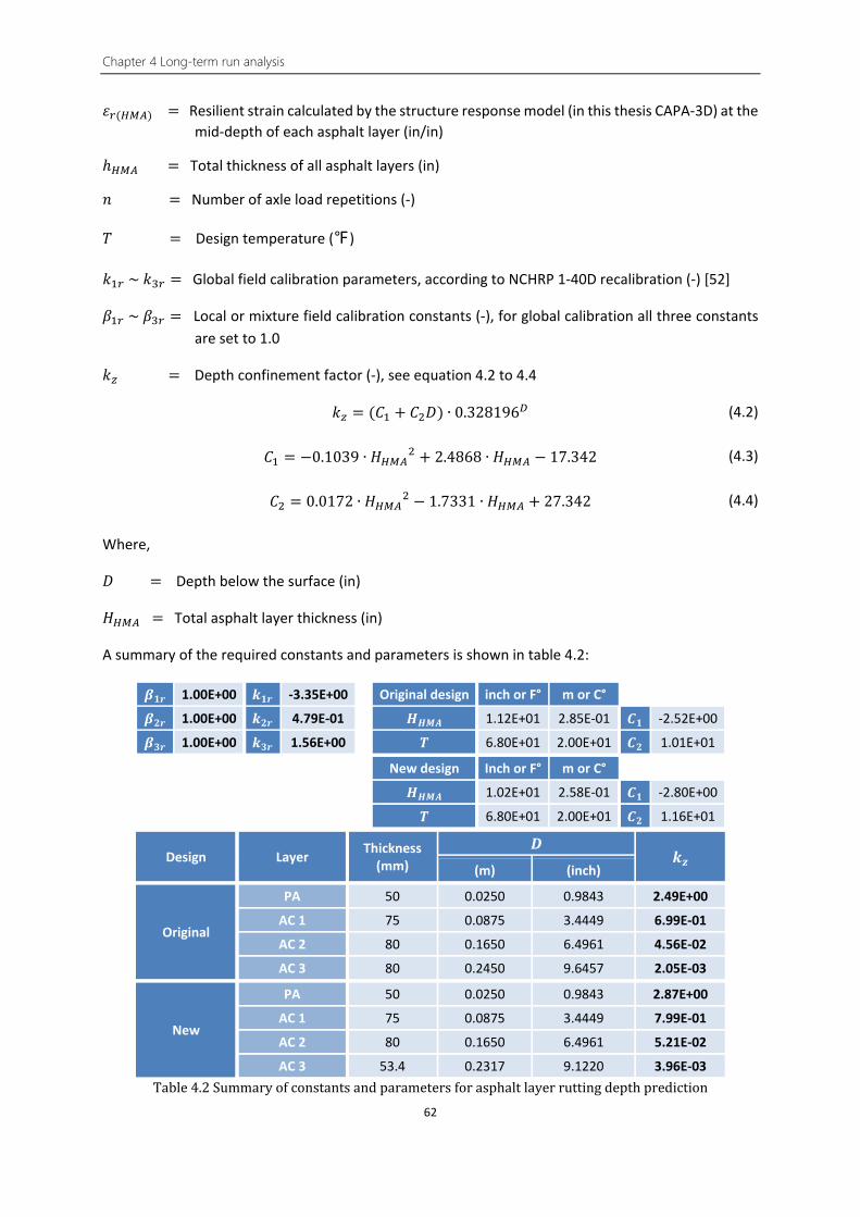
Chapter 4 Long-term run analysis
62
𝜀𝜀𝑛𝑛(𝐻𝐻𝐻𝐻𝐴𝐴) = Resilient strain calculated by the structure response model (in this thesis CAPA-3D) at the mid-depth of each asphalt layer (in/in)
ℎ𝐻𝐻𝐻𝐻𝐴𝐴 = Total thickness of all asphalt layers (in)
𝑛𝑛 = Number of axle load repetitions (-)
𝑇𝑇 = Design temperature (℉)
𝑘𝑘1𝑛𝑛 ~ 𝑘𝑘3𝑛𝑛 = Global field calibration parameters, according to NCHRP 1-40D recalibration (-) [52]
𝛽𝛽1𝑛𝑛 ~ 𝛽𝛽3𝑛𝑛 = Local or mixture field calibration constants (-), for global calibration all three constants are set to 1.0
𝑘𝑘𝑜𝑜 = Depth confinement factor (-), see equation 4.2 to 4.4
𝑘𝑘𝑜𝑜 = (𝐶𝐶1 + 𝐶𝐶2𝐷𝐷) ∙ 0.328196𝐷𝐷 (4.2)
𝐶𝐶1 = −0.1039 ∙ 𝐻𝐻𝐻𝐻𝐻𝐻𝐴𝐴2 + 2.4868 ∙ 𝐻𝐻𝐻𝐻𝐻𝐻𝐴𝐴 − 17.342 (4.3)
𝐶𝐶2 = 0.0172 ∙ 𝐻𝐻𝐻𝐻𝐻𝐻𝐴𝐴2 − 1.7331 ∙ 𝐻𝐻𝐻𝐻𝐻𝐻𝐴𝐴 + 27.342 (4.4)
Where,
𝐷𝐷 = Depth below the surface (in)
𝐻𝐻𝐻𝐻𝐻𝐻𝐴𝐴 = Total asphalt layer thickness (in)
A summary of the required constants and parameters is shown in table 4.2:
𝜷𝜷𝟏𝟏𝑶𝑶 1.00E+00 𝒌𝒌𝟏𝟏𝑶𝑶 -3.35E+00 Original design inch or F° m or C°
𝜷𝜷𝟐𝟐𝑶𝑶 1.00E+00 𝒌𝒌𝟐𝟐𝑶𝑶 4.79E-01 𝑯𝑯𝑯𝑯𝑴𝑴𝑯𝑯 1.12E+01 2.85E-01 𝑪𝑪𝟏𝟏 -2.52E+00
𝜷𝜷𝟑𝟑𝑶𝑶 1.00E+00 𝒌𝒌𝟑𝟑𝑶𝑶 1.56E+00 𝑻𝑻 6.80E+01 2.00E+01 𝑪𝑪𝟐𝟐 1.01E+01 New design Inch or F° m or C°
𝑯𝑯𝑯𝑯𝑴𝑴𝑯𝑯 1.02E+01 2.58E-01 𝑪𝑪𝟏𝟏 -2.80E+00 𝑻𝑻 6.80E+01 2.00E+01 𝑪𝑪𝟐𝟐 1.16E+01
Design Layer Thickness (mm)
𝑫𝑫 𝒌𝒌𝒛𝒛
(m) (inch)
Original
PA 50 0.0250 0.9843 2.49E+00
AC 1 75 0.0875 3.4449 6.99E-01
AC 2 80 0.1650 6.4961 4.56E-02
AC 3 80 0.2450 9.6457 2.05E-03
New
PA 50 0.0250 0.9843 2.87E+00
AC 1 75 0.0875 3.4449 7.99E-01
AC 2 80 0.1650 6.4961 5.21E-02
AC 3 53.4 0.2317 9.1220 3.96E-03 Table 4.2 Summary of constants and parameters for asphalt layer rutting depth prediction

4.1 Real-life simulation
63
For the unbound material layers, the rutting depth of subgrade and other unbound layers are
calculated separately.
The initial model used to predict the permanent deformation of unbound layers was proposed by
Tseng and Lytton in 1989 [53]. The basic relationship is:
Δ𝑠𝑠(𝑠𝑠𝑏𝑏𝑏𝑏𝑣𝑣𝑠𝑠𝑏𝑏𝑑𝑑) = ��𝜀𝜀0 ∙ 𝑒𝑒−�𝜌𝜌𝑁𝑁�
𝛽𝛽
� ∙ 𝛽𝛽1 ∙ �𝜀𝜀𝑣𝑣𝜀𝜀𝑛𝑛�� ∙ ℎ = 𝛽𝛽1 ∙ �
𝜀𝜀0𝜀𝜀𝑛𝑛� ∙ 𝑒𝑒−�
𝜌𝜌𝑁𝑁�
𝛽𝛽
∙ 𝜀𝜀𝑣𝑣 ∙ ℎ (4.5)
Where,
Δ𝑠𝑠(𝑠𝑠𝑏𝑏𝑏𝑏𝑣𝑣𝑠𝑠𝑏𝑏𝑑𝑑) = Permanent deformation of unbound layer (in)
𝜀𝜀0,𝛽𝛽 & 𝜌𝜌 = Material properties (-)
𝑁𝑁 = Number of axle load repetitions (-)
𝜀𝜀𝑛𝑛 = Resilient strain imposed in laboratory test to obtain the above listed material properties (in/in)
𝜀𝜀𝑣𝑣 = Average vertical resilient strain in the unbound layer as obtained from the primary response model (in/in)
ℎ = Thickness of the unbound layer (in);
𝛽𝛽1 = Calibration factor for the unbound materials (-)
The ratio is estimated upon the type of the material. Many models have been developed and modified
to derive this ratio. For the upper unbound layers, the final chosen approach is shown in a series of
equations:
log𝛽𝛽 = −0.61119 − 0.017638 ∙ 𝑊𝑊𝑠𝑠 (4.6)
�𝜀𝜀0𝜀𝜀𝑛𝑛� =
�𝑑𝑑𝜌𝜌𝛽𝛽∙𝑏𝑏1∙𝐸𝐸𝑛𝑛
𝑏𝑏1�+(𝑑𝑑� 𝜌𝜌109
�𝛽𝛽
∙𝑏𝑏9∙𝐸𝐸𝑛𝑛𝑏𝑏9)
2 (4.7)
𝐶𝐶0 = ln �(𝑏𝑏1∙𝐸𝐸𝑛𝑛𝑏𝑏1)
(𝑏𝑏9∙𝐸𝐸𝑛𝑛𝑏𝑏9)� (4.8)
𝜌𝜌 = 109 � 𝐶𝐶01−(109)𝛽𝛽
�1𝛽𝛽 (4.9)
𝑊𝑊𝑠𝑠 = 51.712 ∙ �� 𝐸𝐸𝑛𝑛2555
�1
0.64�−0.3586∙𝐺𝐺𝐺𝐺𝑁𝑁0.1192
(4.10)
Where,

Chapter 4 Long-term run analysis
64
𝑎𝑎1, 𝑏𝑏1 & 𝑎𝑎9, 𝑏𝑏9 = Traffic level related parameters (-), solved for N=1 and N=109 respectively. Here, 𝑎𝑎1 = 0.15, 𝑏𝑏1 = 0.0, 𝑎𝑎9 = 20.0, 𝑏𝑏9 = 0.0 [52]
𝑊𝑊𝑠𝑠 = Water content (%)
𝜏𝜏𝑛𝑛 = Resilient modulus of the unbound material (psi)
𝐺𝐺𝑊𝑊𝑇𝑇 = Ground water table depth (ft). In the Netherlands the ground water level varies from 0.5 to 1.0 metre below the surface in the western part of the country, while in the higher area from 1.0 to 20.0 metres [54]. In this thesis a GWT of 1.0 metre is chosen for the calculation
The subgrade of the pavement usually possesses very large depth and in some cases, for example the
Dutch design method, is considered to be a semi-infinite layer. Therefore the procedure of the
determination of permanent deformation in the upper unbound layers is no longer applicable. An
alternative method has been developed to evaluate the plastic strain for an infinite layer as noted
down below:
ε𝑠𝑠(𝑧𝑧) = (ε𝑠𝑠,𝑜𝑜=0) ∙ 𝑒𝑒−𝑘𝑘𝑜𝑜 (4.11)
Where,
ε𝑠𝑠(𝑧𝑧) = Plastic vertical strain at depth z ((in/in)), measured from the top of the subgrade
ε𝑠𝑠,𝑜𝑜=0 = Plastic vertical strain at the top (z=0) of the subgrade (in/in)
𝑧𝑧 = Depth measured from the top of the subgrade (ft)
𝑘𝑘 = Constant obtained from regression (-)
The resilient strains at the top of the subgrade and at the depth of 6 inches from the top of the
subgrade can be obtained from the real-life simulation. The requisite parameters, �𝜀𝜀0𝜀𝜀𝑛𝑛�, β and ρ, at the
two depth can be calculated separately using the procedure mentioned earlier for unbound materials.
Then the plastic vertical strain for both depth can be computed as:
ε𝑠𝑠 = �𝜀𝜀0𝜀𝜀𝑛𝑛� ∙ 𝑒𝑒−�
𝜌𝜌𝑁𝑁�
𝛽𝛽
∙ ε𝑣𝑣 (4.12)
Where,
ε𝑣𝑣 = Resilient strain output from the real-life simulation (in/in)
𝑁𝑁 = Number of axle load repetitions (-)
Using these two data points, the regression constant can be solved as:
k = 16
ln (ε𝑠𝑠,𝑧𝑧=0
ε𝑠𝑠,𝑧𝑧=6) (4.13)
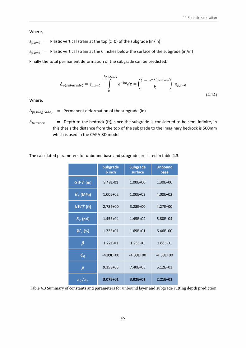
4.1 Real-life simulation
65
Where,
ε𝑠𝑠,𝑜𝑜=0 = Plastic vertical strain at the top (z=0) of the subgrade (in/in)
ε𝑠𝑠,𝑜𝑜=6 = Plastic vertical strain at the 6 inches below the surface of the subgrade (in/in)
Finally the total permanent deformation of the subgrade can be predicted:
Δ𝑠𝑠(𝑠𝑠𝑠𝑠𝑏𝑏𝑒𝑒𝑛𝑛𝑏𝑏𝑑𝑑𝑑𝑑) = ε𝑠𝑠,𝑜𝑜=0 ∙ � 𝑒𝑒−𝑘𝑘𝑜𝑜𝑑𝑑𝑧𝑧 = �1 − 𝑒𝑒−𝑘𝑘ℎ𝑏𝑏𝑡𝑡𝑏𝑏𝑛𝑛𝑛𝑛𝑏𝑏𝑏𝑏
𝑘𝑘�
ℎ𝑏𝑏𝑡𝑡𝑏𝑏𝑛𝑛𝑛𝑛𝑏𝑏𝑏𝑏
0
∙ ε𝑠𝑠,𝑜𝑜=0
(4.14) Where,
Δ𝑠𝑠(𝑠𝑠𝑠𝑠𝑏𝑏𝑒𝑒𝑛𝑛𝑏𝑏𝑑𝑑𝑑𝑑) = Permanent deformation of the subgrade (in)
ℎ𝑏𝑏𝑑𝑑𝑑𝑑𝑛𝑛𝑣𝑣𝑠𝑠𝑘𝑘 = Depth to the bedrock (ft), since the subgrade is considered to be semi-infinite, in this thesis the distance from the top of the subgrade to the imaginary bedrock is 500mm which is used in the CAPA-3D model
The calculated parameters for unbound base and subgrade are listed in table 4.3.
Subgrade 6 inch
Subgrade surface
Unbound base
𝑮𝑮𝑮𝑮𝑻𝑻 (m) 8.48E-01 1.00E+00 1.30E+00
𝑬𝑬𝑶𝑶 (MPa) 1.00E+02 1.00E+02 4.00E+02
𝑮𝑮𝑮𝑮𝑻𝑻 (ft) 2.78E+00 3.28E+00 4.27E+00
𝑬𝑬𝑶𝑶 (psi) 1.45E+04 1.45E+04 5.80E+04
𝑮𝑮𝒄𝒄 (%) 1.72E+01 1.69E+01 6.46E+00
𝜷𝜷 1.22E-01 1.23E-01 1.88E-01
𝑪𝑪𝟎𝟎 -4.89E+00 -4.89E+00 -4.89E+00
𝝆𝝆 9.35E+05 7.40E+05 5.12E+03
𝜺𝜺𝟎𝟎 𝜺𝜺𝑶𝑶⁄ 3.07E+01 3.02E+01 2.21E+01
Table 4.3 Summary of constants and parameters for unbound layer and subgrade rutting depth prediction
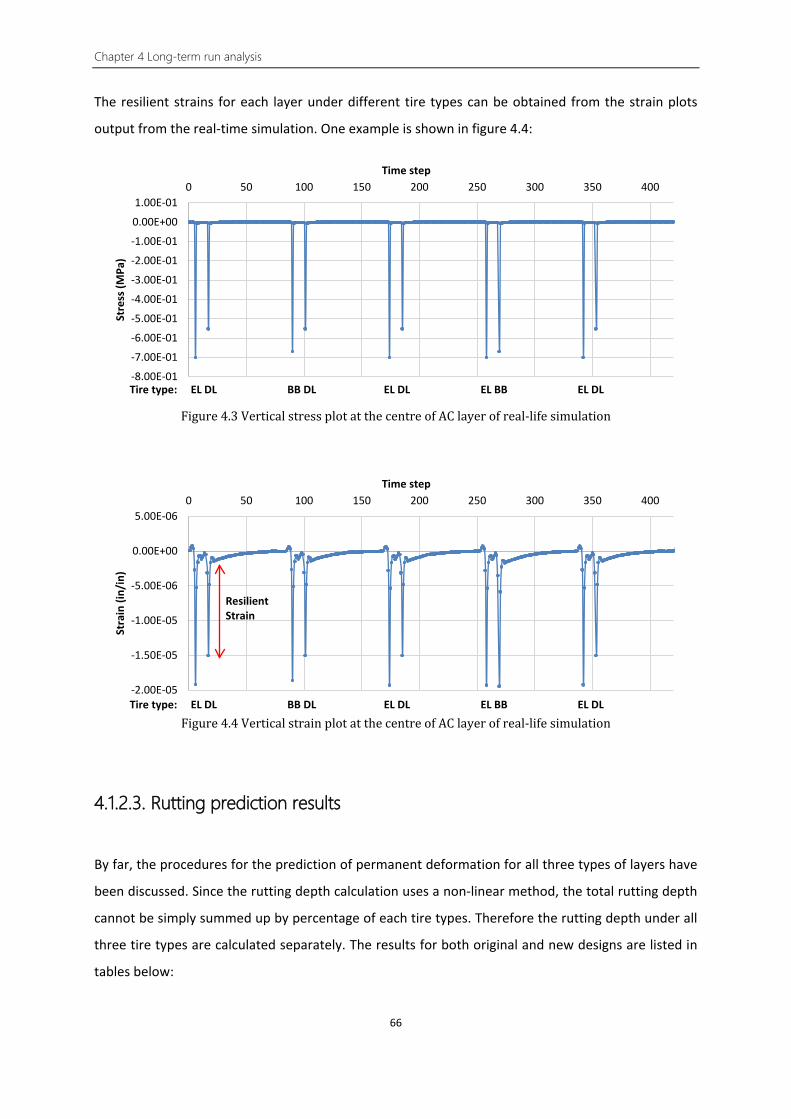
Chapter 4 Long-term run analysis
66
The resilient strains for each layer under different tire types can be obtained from the strain plots
output from the real-time simulation. One example is shown in figure 4.4:
Figure 4.3 Vertical stress plot at the centre of AC layer of real-life simulation
Figure 4.4 Vertical strain plot at the centre of AC layer of real-life simulation
4.1.2.3. Rutting prediction results
By far, the procedures for the prediction of permanent deformation for all three types of layers have
been discussed. Since the rutting depth calculation uses a non-linear method, the total rutting depth
cannot be simply summed up by percentage of each tire types. Therefore the rutting depth under all
three tire types are calculated separately. The results for both original and new designs are listed in
tables below:
-8.00E-01
-7.00E-01
-6.00E-01
-5.00E-01
-4.00E-01
-3.00E-01
-2.00E-01
-1.00E-01
0.00E+00
1.00E-010 50 100 150 200 250 300 350 400
Stre
ss (M
Pa)
Time step
-2.00E-05
-1.50E-05
-1.00E-05
-5.00E-06
0.00E+00
5.00E-060 50 100 150 200 250 300 350 400
Stra
in (i
n/in
)
Time step
Tire type: EL DL BB DL EL DL EL BB EL DL
Resilient Strain
Tire type: EL DL BB DL EL DL EL BB EL DL

4.1 Real-life simulation
67
Single tire (EL)
Design Original New
𝚫𝚫% Layer 𝜺𝜺𝑶𝑶
(in/in)
𝚫𝚫𝒑𝒑 % 𝜺𝜺𝑶𝑶
(in/in)
𝚫𝚫𝒑𝒑 %
(inch) (mm) (inch) (mm)
PA 7.91E-05 0.3220 8.1800 82.67% 7.54E-05 0.3530 8.9700 82.39% 9.68%
AC 1 1.03E-05 0.0117 0.2980 3.01% 8.49E-06 0.0111 0.2810 2.58% -5.72%
AC 2 1.25E-05 0.0009 0.0236 0.24% 1.37E-05 0.0012 0.0296 0.27% 25.66%
AC 3 1.58E-05 0.0001 0.0013 0.01% 1.98E-05 0.0001 0.0033 0.03% 142.89%
AC 0.0127 0.3230 3.26% 0.0123 0.3140 2.88% -2.81%
Asphalt 0.3350 8.5000 85.93% 0.3650 9.2800 85.27% 9.20%
Unbound base 4.84E-05 0.0112 0.2830 2.86% 5.63E-05 0.0141 0.3590 3.30% 26.65%
Subgrade z=0 1.14E-04 0.0026 0.0656 1.29E-04 0.0029 0.0743
Subgrade z=6 1.04E-04 0.0024 0.0596 1.17E-04 0.0026 0.0671
k 0.0159 0.0169
Subgrade 0.0436 1.1100 11.21% 0.0490 1.2400 11.43% 12.23%
ΣΔ 0.3890 9.8890 0.4280 10.8830 10.04%
Table 4.4 Pavement rutting depth prediction under Single tire (EL)

Chapter 4 Long-term run analysis
68
Dual tire (DL)
Design Original New
𝚫𝚫% Layer 𝜺𝜺𝑶𝑶
(in/in)
𝚫𝚫𝒑𝒑 % 𝜺𝜺𝑶𝑶
(in/in)
𝚫𝚫𝒑𝒑 %
(inch) (mm) (inch) (mm)
PA 7.16E-05 0.2913 7.3994 82.05% 6.89E-05 0.3225 8.1903 81.90% 10.69%
AC 1 8.36E-06 0.0095 0.2419 2.68% 7.28E-06 0.0095 0.2409 2.41% -0.42%
AC 2 9.01E-06 0.0007 0.0170 0.19% 1.02E-05 0.0009 0.0219 0.22% 29.00%
AC 3 1.20E-05 0.0000 0.0010 0.01% 1.50E-05 0.0001 0.0025 0.02% 141.53%
AC 0.0102 0.2599 2.88% 0.0104 0.2653 2.65% 2.06%
Asphalt 0.3015 7.6593 84.93% 0.3329 8.4556 84.55% 10.40%
Unbound base 4.41E-05 0.0102 0.2582 2.86% 5.07E-05 0.0127 0.3590 3.59% 39.04%
Subgrade z=0 1.11E-04 0.0025 0.0636 1.24E-04 0.0028 0.0743
Subgrade z=6 1.03E-04 0.0023 0.0587 1.14E-04 0.0026 0.0671
k 0.0133 0.0144
Subgrade 0.0433 1.1008 12.21% 0.0481 1.2220 12.22% 11.00%
ΣΔ 0.3551 9.0183 0.3937 10.0003 10.89%
Table 4.5 Pavement rutting depth prediction under Dual tire (DL)
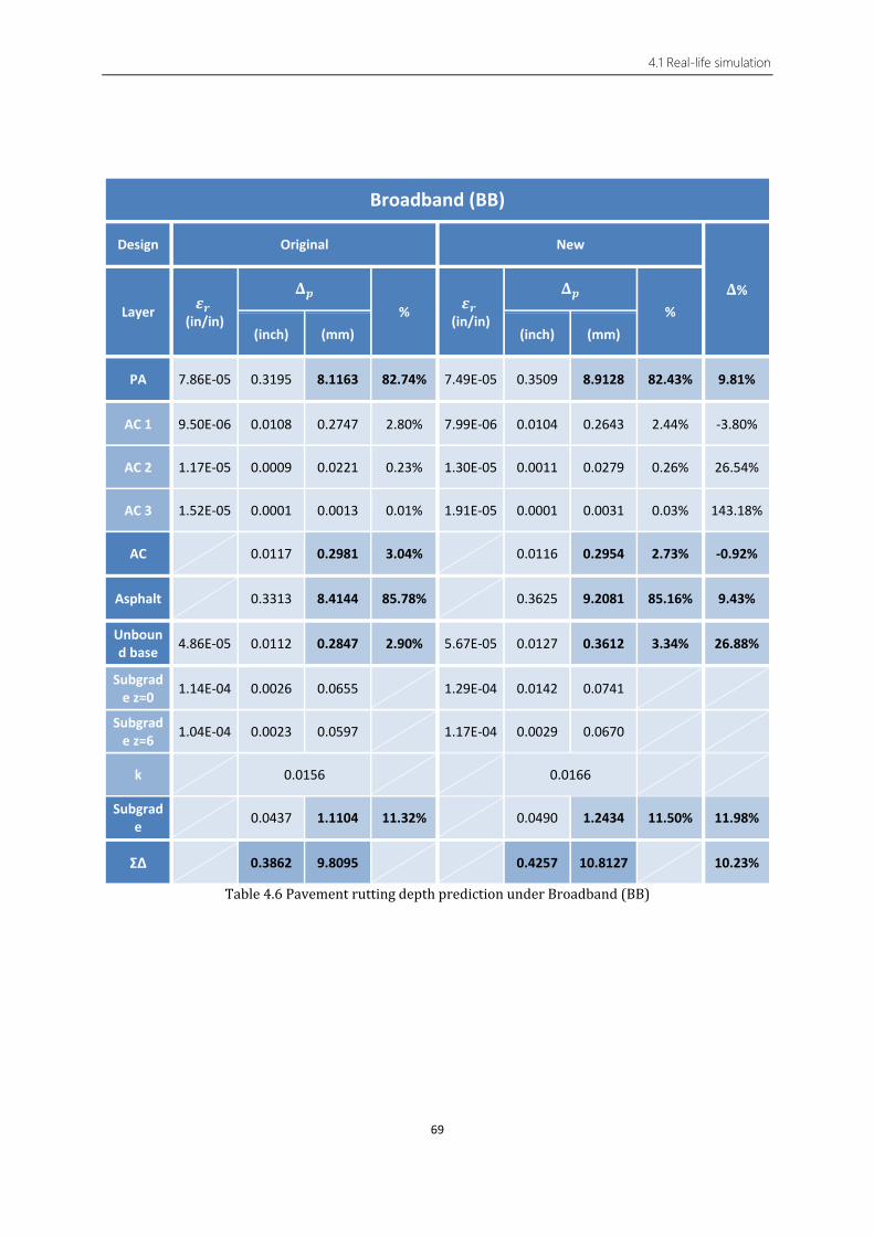
4.1 Real-life simulation
69
Broadband (BB)
Design Original New
𝚫𝚫% Layer 𝜺𝜺𝑶𝑶
(in/in)
𝚫𝚫𝒑𝒑 % 𝜺𝜺𝑶𝑶
(in/in)
𝚫𝚫𝒑𝒑 %
(inch) (mm) (inch) (mm)
PA 7.86E-05 0.3195 8.1163 82.74% 7.49E-05 0.3509 8.9128 82.43% 9.81%
AC 1 9.50E-06 0.0108 0.2747 2.80% 7.99E-06 0.0104 0.2643 2.44% -3.80%
AC 2 1.17E-05 0.0009 0.0221 0.23% 1.30E-05 0.0011 0.0279 0.26% 26.54%
AC 3 1.52E-05 0.0001 0.0013 0.01% 1.91E-05 0.0001 0.0031 0.03% 143.18%
AC 0.0117 0.2981 3.04% 0.0116 0.2954 2.73% -0.92%
Asphalt 0.3313 8.4144 85.78% 0.3625 9.2081 85.16% 9.43%
Unbound base 4.86E-05 0.0112 0.2847 2.90% 5.67E-05 0.0127 0.3612 3.34% 26.88%
Subgrade z=0 1.14E-04 0.0026 0.0655 1.29E-04 0.0142 0.0741
Subgrade z=6 1.04E-04 0.0023 0.0597 1.17E-04 0.0029 0.0670
k 0.0156 0.0166
Subgrade 0.0437 1.1104 11.32% 0.0490 1.2434 11.50% 11.98%
ΣΔ 0.3862 9.8095 0.4257 10.8127 10.23%
Table 4.6 Pavement rutting depth prediction under Broadband (BB)

Chapter 4 Long-term run analysis
70
4.1.3. Rutting prediction comparison
The rutting depth results of all three tire types share the same pattern. For the total rutting depth, the
new designed pavement structure indeed suffers a more severe deformation. However this increase
is not as significant as the boost of fatigue prediction. The new design leads to a roughly 10% increase
for all three tire types.
When zooming into the rutting depth of each layer respectively, the top layer (PA layer) undoubtedly
hold the dominant position with a nearly 82% contribution of the total rutting depth. In the new design
the resilient strain of the PA layer increases. Since the thickness of this layer remains the same, a 10%
increase of the rutting depth is produced.
For the AC layer, although the resilient strains fluctuate due to the thickness change, the reduction of
the thickness in this layer to some extent neutralizes the strain increase. As a result the original and
new design almost share the same rutting depth in the AC layer.
On the contrary, in the unbound base layer, the reduction of the AC layer leads to an increase of the
resilient strain. Plus the extra thickness assigned to this layer, the unbound base layer suffers the
biggest increase percentage around 26%.
Finally the subgrade has the same change pattern as the PA layer. With increased resilient strains and
non-changed layer thickness, a 12% rise is witnessed in the rutting depth of the subgrade.
It is also worth noticing that although the rutting depth prediction of the new design indeed increases,
which indicates a positive result in material cost-efficiency, there is still a significant gap to the rutting
depth prediction of the heavy traffic lane. If the pavement is evaluated solely based on this criterion,
there is still more potential for reduction of thickness in the light traffic lanes.
4.1.4. Real-life simulation deformation output
The deformation plots of the real-life simulation are shown below.
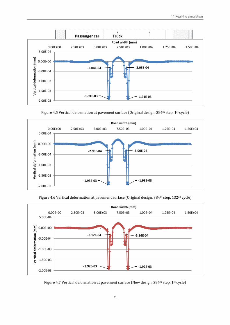
4.1 Real-life simulation
71
Figure 4.5 Vertical deformation at pavement surface (Original design, 384th step, 1st cycle)
Figure 4.6 Vertical deformation at pavement surface (Original design, 384th step, 132nd cycle)
Figure 4.7 Vertical deformation at pavement surface (New design, 384th step, 1st cycle)
-1.91E-03
-3.04E-04 -3.05E-04
-1.91E-03-2.00E-03
-1.50E-03
-1.00E-03
-5.00E-04
0.00E+00
5.00E-040.00E+00 2.50E+03 5.00E+03 7.50E+03 1.00E+04 1.25E+04 1.50E+04
Vert
ical
def
orm
atio
n (m
m)
Road width (mm)
-1.93E-03
-2.99E-04 -3.00E-04
-1.93E-03
-2.00E-03
-1.50E-03
-1.00E-03
-5.00E-04
0.00E+00
5.00E-040.00E+00 2.50E+03 5.00E+03 7.50E+03 1.00E+04 1.25E+04 1.50E+04
Vert
ical
def
orm
atio
n (m
m)
Road width (mm)
-1.92E-03
-3.12E-04 -3.16E-04
-1.92E-03-2.00E-03
-1.50E-03
-1.00E-03
-5.00E-04
0.00E+00
5.00E-040.00E+00 2.50E+03 5.00E+03 7.50E+03 1.00E+04 1.25E+04 1.50E+04
Vert
ical
def
orm
atio
n (m
m)
Road width (mm)
Passenger car Truck

Chapter 4 Long-term run analysis
72
Figure 4.8 Vertical deformation at pavement surface (New design, 384th step, 132nd cycle)
Figure 4.5 & 4.6 and 4.7 & 4.8 show the vertical deformation at the surface of the pavement of the 1st
load cycle and the 67th cycle for both original and new design. As time goes by, the accumulated vertical
deformation indeed occurs in both cases. As predicted the new design produces larger deformation
than the original design since the thickness of asphalt layer is reduced in the outer and middle lanes
(left two lanes). Moreover, the slope structure design in the new design indeed affects the vertical
deformation distribution across the pavement. However this influence is limited which will not
negatively affect the driving experience on this lane. Both original and new designs share the same
growth rates.
Position Deformation (mm)
Growth value Growth rate 1st cycle 132nd cycle
Original design
Tire edge 1 -1.91E-03 -1.93E-03 1.77E-05 0.93%
Gap centre 1 -3.04E-04 -2.99E-04 4.47E-06 1.47%
Gap centre 2 -3.05E-04 -3.00E-04 4.48E-06 1.47%
Tire edge 2 -1.91E-03 -1.93E-03 1.77E-05 0.93%
New design
Tire edge 1 -1.92E-03 -1.93E-03 1.77E-05 0.92%
Gap centre 1 -3.12E-04 -3.08E-04 4.49E-06 1.44%
Gap centre 2 -3.16E-04 -3.12E-04 4.48E-06 1.42%
Tire edge 2 -1.92E-03 -1.94E-03 1.77E-05 0.92% Table 4.7 Vertical deformation growth at critical positions (Original vs New design)
-1.93E-03
-3.08E-04 -3.12E-04
-1.94E-03-2.00E-03
-1.50E-03
-1.00E-03
-5.00E-04
0.00E+00
5.00E-040.00E+00 2.50E+03 5.00E+03 7.50E+03 1.00E+04 1.25E+04 1.50E+04
Vert
ical
def
orm
atio
n (m
m)
Road width (mm)Passenger car Truck
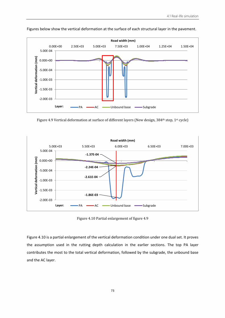
4.1 Real-life simulation
73
Figures below show the vertical deformation at the surface of each structural layer in the pavement.
Figure 4.9 Vertical deformation at surface of different layers (New design, 384th step, 1st cycle)
Figure 4.10 Partial enlargement of figure 4.9
Figure 4.10 is a partial enlargement of the vertical deformation condition under one dual set. It proves
the assumption used in the rutting depth calculation in the earlier sections. The top PA layer
contributes the most to the total vertical deformation, followed by the subgrade, the unbound base
and the AC layer.
-2.00E-03
-1.50E-03
-1.00E-03
-5.00E-04
0.00E+00
5.00E-040.00E+00 2.50E+03 5.00E+03 7.50E+03 1.00E+04 1.25E+04 1.50E+04
Vert
ical
def
orm
atio
n (m
m)
Road width (mm)
PA AC Unbound base Subgrade
-1.86E-03
-2.61E-04
-2.24E-04
-1.37E-04
-2.00E-03
-1.50E-03
-1.00E-03
-5.00E-04
0.00E+00
5.00E-045.00E+03 5.50E+03 6.00E+03 6.50E+03 7.00E+03
Vert
ical
def
orm
atio
n (m
m)
Road width (mm)
PA AC Unbound base Subgrade
Layer:
Layer:

Chapter 4 Long-term run analysis
74
Layer Surface positon (mm)
Total deformation
(mm)
Deformation per layer
(mm) Percentage Calculated
percentage
PA 1.09E+03 -1.86E-03 -1.60E-03 85.97% 82.39%
AC 1.04E+03 -2.61E-04 -3.70E-05 1.99% 2.88%
Unbound base
8.28E+02 -2.24E-04 -8.70E-05 4.67% 3.30%
Subgrade 5.00E+02 -1.37E-04 -1.37E-04 7.37% 11.43%
Table 4.8 Vertical deformation contribution of each layer
The results support the concept that the rutting depth of the pavement is an accumulation of the
deformations in all layers, from top to bottom, of the entire pavement structure. Therefore it is
recommended that for the future pavement structure design the permanent deformation evaluation
should consider the rutting condition in all the layers rather than only focusing on the subgrade or
unbound layers.
4.1.5. Criticism on the deformation analysis
In the previous sections both MEPDG calculation and real-life simulation output indicated that the top
PA layer would produce the largest vertical deformation. However, in practice it is hardly the case.
Porous asphalt (PA) uses an open-graded aggregate to obtain high air voids which provide the ability
of quickly removing the water from the pavement surface. Meanwhile open-graded aggregate also
leads to a coarse granular skeleton with more stone-on-stone contact since there is limited fine
aggregate or asphalt binder comparing to AC (figure 4.11). The skeleton of larger stones resists traffic
loads by transmitting them through stone-on-stone contact and eventually to the layers below. As a
result, the deformation or rutting resistant capacity of PA is better than AC [67].
However in both MEPDG method and the finite element models, the materials are considered to be
isotropic and homogeneous. So does the Dutch design software OIA. The strain response as well as
deformation are calculated almost solely based on the stiffness. Since the stiffness of PA is smaller
than AC, the top layer is predicted to produce the largest vertical deformation.

4.2 Platooning
75
Figure 4.11 Schematic presentation of pavement materials commonly used I the Netherlands [68]
Furthermore, theoretically the deformation plots here can never be the “permanent” deformation. In
the real-life simulation the axle loads are constantly passing by on the pavement. For example figure
4.9 shows the 384th time step in the 1 loading cycle. It means the plot represents the deformation
situation after the last axle passing by during the 348th to 357th time step. Hence the pavement is still
recovering from the deformation causing by the past axle load. In fact since in the simulation all
materials are elastic or viscoelastic (generalized Maxwell model), if the pavement is given long enough
time to relax, in the end all the deformation will disappear. As a result here figure 4.8 shows more
likely the instant deformation under the passing loads (or primary deformation) rather than the
permanent deformation.
4.2. Platooning
In Europe, truck platooning has become a hot research topic and industrial opportunity. A truck
platoon consist of several trucks driven closely one by one with the help of a modern communicating
and navigating system. Since the distance between the trucks is relatively smaller, the different strain
condition in the pavement is worth studying [55].
With the proper traffic, pavement geometry and material parameter input, almost any traffic condition
can be simulated and compared by using the established model in CAPA-3D. In this section a simple
simulation and comparison of truck platooning on the pavement structure is executed.

Chapter 4 Long-term run analysis
76
4.2.1. Background
Truck platooning comprises a row of trucks equipped with an advanced driving support system which
enables the trucks to follow each other with a much closer safe distance. As mentioned in the former
chapter, in many countries, including the Netherlands, the regulated minimum safe distance between
vehicles is defined by two parts in the form of time: reaction time and braking time. In a truck platoon,
with a zero reaction thanks to the system, the following trucks are able to brake immediately which
can help improve traffic safety with even a shorter safety distance. Platooning also has the potential
of cost saving since trucks are driven closer to each other at a same speed which will lower the fuel
consumption as well as the CO2 emissions. Lastly, platooning also efficiently enhances the traffic flows
resulting in a reduction of traffic jams [56].
All the advantages mentioned above are almost all based on the fact that truck platooning will lead to
a more frequent, constant loading on the pavement with a shorter relaxing time. This may cause a
different strain reaction of the pavement structure and lead to a different performance prediction.
Hence it is worth investigating it with the help of the finite element model.
4.2.2. Data Input
Since in most of the present platooning field tests the trucks in a platoon hold the same specifications,
and also to simplify the input, only one type of axle load, which is dual tire with a vertical load of 100
kN, is applied in this platooning simulation. A longer truck model with a wheelbase of 11 metres is
applied to mimic the standard shipping container truck used in the field test hence the time interval
between the front and rear axles is 0.5 second [34]. The following distance between trucks in
platooning is smaller than the regulated safe distance of 2.0 second. European Automobile
Manufacturers' Association (ACEA) set 0.5 second as a minimum following distance for the truck
manufacturers [55]. Finally four trucks are set for one platoon in this simulation.
As for the control test the same truck models are used with a regulated safe distance of 2.0 second.
The total amount of trucks in both tests should be the same. It takes 10 seconds for 4 trucks to pass by
in the normal case, therefore the time interval between two truck platoons is set to 6.5 seconds.
The input data for both cases is listed in figure 4.12.

4.2 Platooning
77
Platooning case (Lane 3)
1st cycle (10.0 s, 400 time steps) 2nd cycle …
1 2 3 4 1 2
…
0.5s 0.5s 0.5s 0.5s 0.5s 0.5s 0.5s 6.5s 0.5s 0.5s 0.5s …
Normal case (Lane 2)
1st cycle (10.0 s, 400 time steps) 2nd cycle …
1 2 3 4 1
…
0.5s 2.0s 0.5s 2.0s 0.5s 2.0s 0.5s 2.0s 0.5s 2.0s …
Figure 4.12 Traffic input for Platooning and Normal case simulation
4.2.3. Data Output and comparison
The plots of horizontal strains at the bottom of the asphalt layer for both normal and platooning cases
in one cycle (four trucks) are shown below:
Figure 4.13 Transverse strain at AC layer bottom (Normal case, 1st cycle)
1.21E+01 1.24E+01 1.21E+01 1.24E+01 1.21E+01 1.24E+01 1.21E+01 1.24E+01
-2.00E-06
0.00E+00
2.00E-06
4.00E-06
6.00E-06
8.00E-06
1.00E-05
1.20E-05
1.40E-05
0 50 100 150 200 250 300 350 400
Tran
sver
se st
rain
(μm
/m)
Time step
+01
+01
+01
+00
+00
+00
+00
+00
+00

Chapter 4 Long-term run analysis
78
Figure 4.14 Transverse strain at AC layer bottom (Platooning case, 1st cycle)
Figure 4.15 Longitudinal strain at AC layer bottom (Normal case, 1st cycle)
Figure 4.16 Longitudinal strain at AC layer bottom (Platooning case, 1st cycle)
1.21E+01 1.24E+01 1.25E+01 1.25E+01
-2.00E-06
0.00E+00
2.00E-06
4.00E-06
6.00E-06
8.00E-06
1.00E-05
1.20E-05
1.40E-05
0 50 100 150 200 250 300 350 400
Tran
sver
se st
rain
(μm
/m)
Time step
1.82E+01 1.83E+01 1.82E+01 1.83E+01 1.82E+01 1.82E+01 1.82E+01 1.82E+01
-5.00E-06
0.00E+00
5.00E-06
1.00E-05
1.50E-05
2.00E-05
0 50 100 150 200 250 300 350 400
Long
itudi
nal s
trai
n (μ
m/m
)
Time step
1.82E+01 1.83E+01 1.83E+01
-5.00E-06
0.00E+00
5.00E-06
1.00E-05
1.50E-05
2.00E-05
0 50 100 150 200 250 300 350 400
Long
itudi
nal s
trai
n (μ
m/m
)
Time step
+01
+01
+01
+00
+00
+00
+00
+00
+00
+01
+01
+01
+00
+00
+00
+01
+01
+01
+00
+00
+00

4.2 Platooning
79
From the plots it can be seen that for the first truck both cases share the same strain pattern. However
for the following trucks, the platooning case produce slight higher strain values while the normal case
continue to repeat the strain pattern of the first truck. The short following time in the platooning case
leaves the pavement a correspondingly shorter recovery time, hence the horizontal strains caused by
the following trucks are larger compared to the normal case. Notice that this response is highly
influenced by the viscoelasticity of the material.
The larger strain in the platooning case means that by the current fatigue prediction procedure used
in chapter 3, the platooning case will cause more severe fatigue problem (larger Miner value) than the
normal case. However since in theory the time interval between two platoons is longer than it in the
normal case, the effect on the recovery or self-healing of the pavement is worth further studies.
The plots of vertical deformation at the surface of the pavement for both normal and platooning cases
at the end of the 1st and 155th cycle are shown below:
Figure 4.17 Vertical deformation at pavement surface (400th step, 1st cycle)
-7.56E-04
1.07E-04 1.06E-04
-7.57E-04
-1.53E-04
5.17E-05 5.57E-05
-1.49E-04
-1.00E-03
-8.00E-04
-6.00E-04
-4.00E-04
-2.00E-04
0.00E+00
2.00E-040.00E+00 2.50E+03 5.00E+03 7.50E+03 1.00E+04 1.25E+04 1.50E+04
Vert
ical
def
orm
atio
n (m
m)
Road width (mm)
Normal case Platooning case
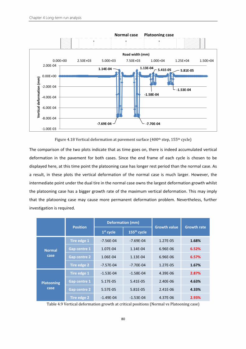
Chapter 4 Long-term run analysis
80
Figure 4.18 Vertical deformation at pavement surface (400th step, 155th cycle)
The comparison of the two plots indicate that as time goes on, there is indeed accumulated vertical
deformation in the pavement for both cases. Since the end frame of each cycle is chosen to be
displayed here, at this time point the platooning case has longer rest period than the normal case. As
a result, in these plots the vertical deformation of the normal case is much larger. However, the
intermediate point under the dual tire in the normal case owns the largest deformation growth whilst
the platooning case has a bigger growth rate of the maximum vertical deformation. This may imply
that the platooning case may cause more permanent deformation problem. Nevertheless, further
investigation is required.
Position Deformation (mm)
Growth value Growth rate 1st cycle 155th cycle
Normal case
Tire edge 1 -7.56E-04 -7.69E-04 1.27E-05 1.68%
Gap centre 1 1.07E-04 1.14E-04 6.96E-06 6.52%
Gap centre 2 1.06E-04 1.13E-04 6.96E-06 6.57%
Tire edge 2 -7.57E-04 -7.70E-04 1.27E-05 1.67%
Platooning case
Tire edge 1 -1.53E-04 -1.58E-04 4.39E-06 2.87%
Gap centre 1 5.17E-05 5.41E-05 2.40E-06 4.63%
Gap centre 2 5.57E-05 5.81E-05 2.41E-06 4.33%
Tire edge 2 -1.49E-04 -1.53E-04 4.37E-06 2.93% Table 4.9 Vertical deformation growth at critical positions (Normal vs Platooning case)
-7.69E-04
1.14E-04 1.13E-04
-7.70E-04
-1.58E-04
5.41E-05 5.81E-05
-1.53E-04
-1.00E-03
-8.00E-04
-6.00E-04
-4.00E-04
-2.00E-04
0.00E+00
2.00E-040.00E+00 2.50E+03 5.00E+03 7.50E+03 1.00E+04 1.25E+04 1.50E+04
Vert
ical
def
orm
atio
n (m
m)
Road width (mm)
Normal case Platooning case
5.1 Construction
81
5. Construction advice and practice feasibility
5.1. Construction
Road construction is a relatively mature industry. Systematic procedures have been established for the
road construction step by step from scratch. In a way, the road construction industry can be somewhat
conservative. Although in the former chapters it has been proven that from the design perspective the
new pavement structure design indeed saves asphaltic materials without compromising its
performance, its feasibility of construction should also be proved.
At present, varies equipment and machines have been developed for certain tasks in the pavement
construction procedure. The road construction is after all a business for both government and
contractors. To earn their support the new design has to be cost efficient for both material saving and
construction cost. It is in their best interest if the new pavement structure design can be implemented
with only the existing equipment and machines.
5.1.1. Existing equipment and machines
The construction of an asphalt pavement has a straightforward procedure to follow. Generally
speaking there are three main steps: preparation of the pavement site, spreading the asphalt mixture,
and compaction of the asphalt mixture [9]. This section will only focus on the equipment and machines
used in each step.
First step: the pavement site should be properly prepared. The subgrade needs to be levelled and
usually compacted to the required density by various types of compaction equipment. On top of the
subgrade an unbound base is placed. The materials are spread by motor graders or bulldozers (dozers).
For drainage purpose the pavement requires a 2% crossfall or crown gradient of the surface. To obtain
this crossfall the surface of the subgrade and unbound base should also have the same slope. This
slope can be accomplished through the final trimming by motor graders [57].

Chapter 5 Construction advice and practice feasibility
82
Figure 5.1 Motor grader (l) and Dozer (r) for pavement site preparation [58]
Second step: the asphalt mixture should be spread onto the base layer with the designed grade,
thickness and slope gradient. A mechanical spreader referred as an asphalt paver or finisher is specially
designed for this task. The most important part of an asphalt paver is the screed. Its primary function
is to lay the asphalt mixture to the designed thickness. Since the screed is able to pivot in a certain
range of angles [59], the slope gradient of the pavement surface is also accomplishable.
Figure 5.2 Asphalt paver for asphalt mixture distribution [58]
Third step: the spread pavement material should be compacted to the desired density to gain the
strength and smoothness. In fact, during the entire pavement construction, in every step, the subgrade,
the unbound base, and the final asphalt mixture all require compaction. Different compactors or rollers
have been developed for different materials. For the asphalt layer, four types of rollers are used: static,
vibratory, pneumatic and a combination thereof [9]. Since in most cases the standard compaction
width of the compactor is smaller than the road width or even the lane width, a rolling pattern with
overlaps between passes is applied.

5.1 Construction
83
Figure 5.3 Static/vibratory roller (l) and Pneumatic roller (r) for compaction [58]
Figure 5.4 Typical rolling pattern [60]
5.1.2. Advice on construction
The cross-section of the new pavement structure design is once again shown in figure 5.5. For a
motorway divided into two individual carriageways for each direction, like this project, a single crossfall
is applied for water runoff instead of a crown.
Median Lane 1 Lane2 Lane 3 Hard shoulder
Figure 5.5 Cross section view of new pavement structural design (m)
Redresseerstrook Marker Marker Redresseerstrook Edge
2%
2% 3%
2%
1,1 0,8 3,25 3,25 0,8 1,65
1,9 10,15 2,95
15
0,53,25
0,2 0,2
Chapter 5 Construction advice and practice feasibility
84
According to the new design, the structural thickness of the third lane (heavy traffic lane) and the hard
shoulder remains the same and therefore can be constructed following the normal procedure whilst
the thickness of the rest part of the asphalt layers is reduced. To be specific only the light traffic parts
of the third asphalt concrete (AC) layer is halved along the diagonal that creates a steeper slope. This
steeper slope is also in favour of drainage. Accordingly the thickness of the unbound base under the
reduced AC layer increases to maintain a “horizontal” pavement surface. Therefore the only
construction challenge is the additional slope at the position between the AC bottom and the unbound
base top.
For the unbound base, the slope can be easily obtained by the motor graders currently used in the
construction. Notice that in the new design the light traffic lane structures are no longer parallel layers.
Instead, in order to facilitate the construction, all the other layers’ surface except the unbound base
remain parallel to the pavement surface as before. Hence the preparation for the subgrade surface
follows the same instruction.
For the AC layer, usually there are upper and lower limits for the allowable paving thickness by an
asphalt layer. The minimum thickness per paving mat should be at least twice or preferable three times
the maximum aggregate size in the asphalt mixture [9]. In this thesis, the maximum aggregate size
used in the AC mixture is 22.4 mm, thus the minimum paving thickness is 67.2 mm. The maximum
paving thickness is not only limited by the specification of the asphalt paver, but also by the ability of
the rollers to obtain the adequate compaction [9]. As a result, the designed thickness of one mixture
is often divided into multiple lifts for asphalt pavers to place. In this project for the original design the
AC layer can be placed in three lifts, one of 75 mm and two of 80 mm, with static wheeled rollers or
two lifts of 120 mm and 115 mm by pneumatic or vibratory rollers whose general thickness limit can
be between 150 and 200 mm [9]. Nevertheless for the new design obviously the latter paving plan is
preferable. The altered slope gradient in the new design can be easily calculated with the result of 1%.
Including the standard 2% crossfall for water runoff, the final total slop gradient is still within the crown
range of any normal asphalt paver [59]. By altering the angle of the screed, the first uneven AC lift can
be placed. At the thinnest point the paving thickness can be set to 70 mm which is higher than the
minimum limit while the thickest point is 150 mm. By doing so a “horizontal” surface of the bottom AC
lift will be accomplished on which another 85 mm parallel AC lift is able to be easily placed following
the routine procedure. This construction design will also help to obtain a more uniform AC layer with
less longitudinal joints.
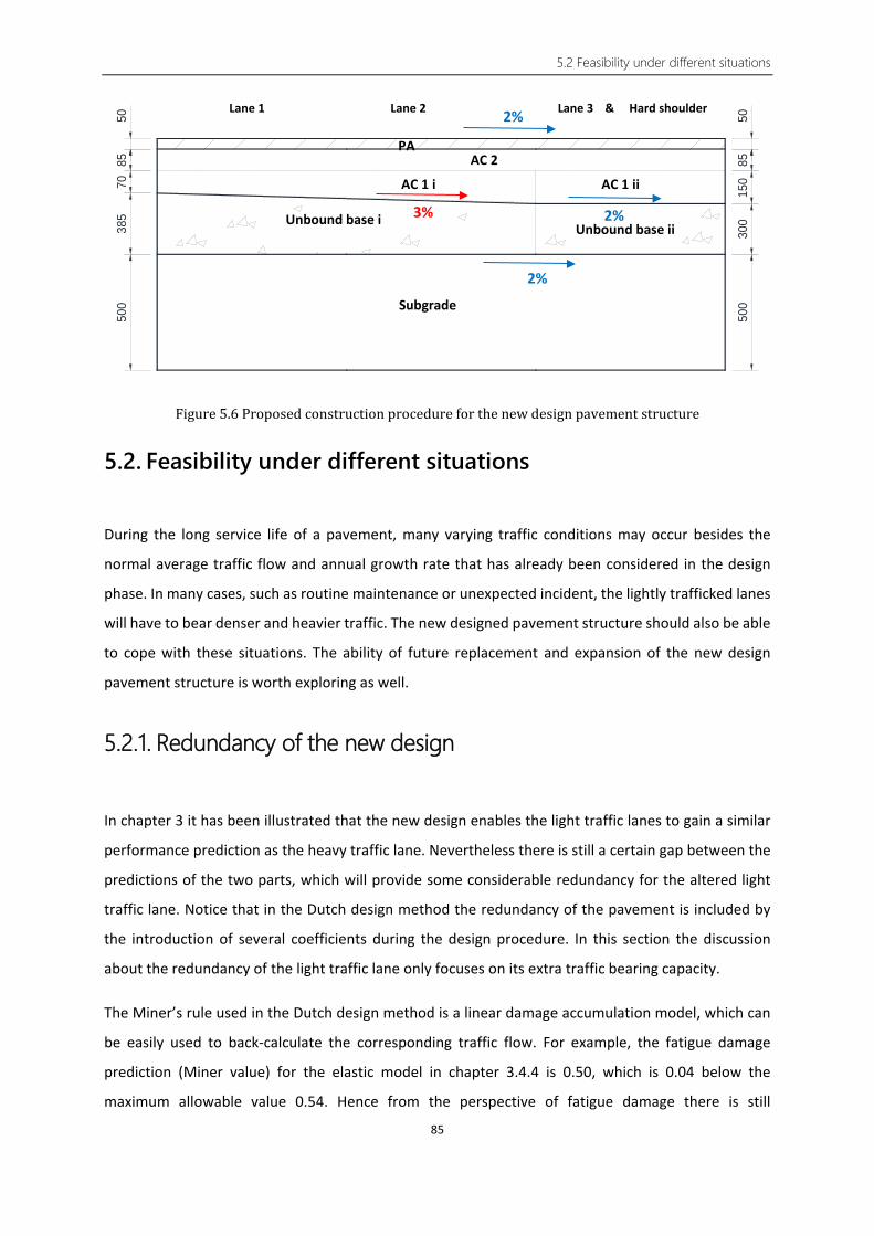
5.2 Feasibility under different situations
85
500
385
7085
50
500
300
150
8550
Figure 5.6 Proposed construction procedure for the new design pavement structure
5.2. Feasibility under different situations
During the long service life of a pavement, many varying traffic conditions may occur besides the
normal average traffic flow and annual growth rate that has already been considered in the design
phase. In many cases, such as routine maintenance or unexpected incident, the lightly trafficked lanes
will have to bear denser and heavier traffic. The new designed pavement structure should also be able
to cope with these situations. The ability of future replacement and expansion of the new design
pavement structure is worth exploring as well.
5.2.1. Redundancy of the new design
In chapter 3 it has been illustrated that the new design enables the light traffic lanes to gain a similar
performance prediction as the heavy traffic lane. Nevertheless there is still a certain gap between the
predictions of the two parts, which will provide some considerable redundancy for the altered light
traffic lane. Notice that in the Dutch design method the redundancy of the pavement is included by
the introduction of several coefficients during the design procedure. In this section the discussion
about the redundancy of the light traffic lane only focuses on its extra traffic bearing capacity.
The Miner’s rule used in the Dutch design method is a linear damage accumulation model, which can
be easily used to back-calculate the corresponding traffic flow. For example, the fatigue damage
prediction (Miner value) for the elastic model in chapter 3.4.4 is 0.50, which is 0.04 below the
maximum allowable value 0.54. Hence from the perspective of fatigue damage there is still
Lane 1 Lane 2 Lane 3 & Hard shoulder
Subgrade
Unbound base i Unbound base ii
AC 1 i AC 1 ii AC 2
PA
2%
3% 2%
2%
Chapter 5 Construction advice and practice feasibility
86
0.04/0.50=8% more traffic flow capacity for the new designed light traffic lane. By multiplying the
current total traffic flow and dividing by the daily traffic flow, the new designed light traffic lane is able
to bear the traffic flow of the heavy traffic lane for an extra period of almost 230 days. Therefore it is
proven that the new design will still hold a certain capability of compensating the abnormal traffic flow
distribution during routine maintenance or unexpected incidents.
5.2.2. Routine maintenance
Maintenance is an essential practice to guarantee the long-term performance and the aesthetic
appearance of the pavement. The purpose of maintenance is to repair the deficiencies caused by
distresses as well as to protect the pavement from further damage [9].
In the Netherlands, regular, annual inspections of the pavement surface are executed all the time. The
data from these inspections then become the input for a damage prediction model developed by
Rijkswaterstraat. Based on the prediction results the so-called preventive maintenance [61] is
performed. The pavement surface will be replaced just before damage is expected. By doing so the
unexpected occurrence of a service or vehicle accident will be prevented and in the long term this
strategy is more cost-efficient than repairing. Since currently in the Netherlands, usually the wearing
course or the upper 50 mm of the pavement is expected to be replaced, the new designed pavement
structure will have no effect on this preventive maintenance.
Meanwhile, other preventative or corrective maintenance is still necessary from time to time to
decrease the rate of deterioration or even correct specific pavement failures or area of distress. These
maintenance activities may include sealcoats, crack or pothole filling, patching, etc. Almost all of these
activities are performed at the surface or upper part of the asphalt layers. Therefore the new designed
pavement structure will also have no effect on these maintenances.
5.2.3. Future expansion
In the Netherlands, road transportation overall has maintained a rising trend over the past decades,
although the 2008 economic crisis slowed down this growth to some extent. The number of cars
continuously increases whilst the year 2016 saw the first increase in the number of vans and heavy
freight vehicles since 2011 [62]. The rising number of vehicles as well as the rate of usage demand a

5.2 Feasibility under different situations
87
larger capacity of the existing motorways. At some point the motorway will have to expand and add
more lanes.
In some newly constructed projects, for instance the Amsterdam – Utrecht part of the A2 motorway,
there is reserved area, usually at the median strip, for future expansion [63]. In this way the
construction site for the future lane has already been prepared for asphalt layers to be placed. For
other cases the expansion has to be situated outside the hard shoulder.
Figure 5.7 Reserved expansion area (median strip) of Rijksweg A2 (Amsterdam – Utrecht) [64]
For the new designed pavement, the latter expansion plan is preferable. Since the outermost (heavy
traffic) lane and the hard shoulder share the same thickness design as the original pavement structure,
the road can be easily expanded following the routine procedure. The expanded lane will have the
same thickness design as the original heavy traffic lane which enables the new road to be more than
adequate for bearing the extra traffic flow.
Figure 5.8 Proposed expansion plan for the new design pavement structure
However, for a new construction project, it is still more cost-efficient to reserve the construction site
at the median strip for future expansion. In this case though the asphalt part thickness of the expanded
Expansion (Median) Lane 1 Lane 2 Lane 3 & Hard shoulder Expansion

Chapter 5 Construction advice and practice feasibility
88
lane should be equal to the thinnest point of the existing passing lane (Lane 1) to maintain the integrity
of the asphalt layer. The expanded lane will become the new passing lane. According to the traffic data
the primary drive for the traffic growth is passenger cars, thus with the expended lane the new road
should also be able to bear the extra traffic flow. Even so, further performance calculation for the
expanded should be applied. In case the prediction result is negative, the overall pavement structure
can still be strengthened by adding an extra asphalt layer on top of the entire road.

6.1 Conclusions
89
6. Conclusions and Recommendations
6.1. Conclusions
The literature review illustrates a brief history of the development of asphalt pavement structures and
design methods. At present the asphalt pavement is constructed as a parallel multi-layer structure with
a uniform thickness design solely based on the chosen design lane regardless the number of lanes the
road contains. However, the traffic data analysis indicates that in practice neither the vehicles amount
nor the axle load classes distribute evenly over different lanes. The structure thickness of the lighter
traffic lanes is clearly overdesigned. Hence a potential of a new material-cost-efficient pavement
structural design is noticed.
Further analysis of the traffic data on Amsterdam – Utrecht section of A2 motorway provided by NDW
proves the uneven distribution of traffic flow over the entire road. The daily traffic amount as well as
axle load classes of each lane are calculated and estimated. Using Dutch asphalt pavement structure
design software OIA, the thickness design of each lane is based on their own traffic data separately. A
considerable reduction of asphalt thickness is observed in the lighter traffic lanes. These thickness
designs are set to be the base of a new structural design for asphalt pavement. To avoid stress
concentration and construction difficulty, a slope design is proposed.
The finite element analysis software, CAPA-3D, is introduced to create a model for the pavement and
execute the simulations. To restrain the model size and running time, a three-lane road with one hard
shoulder is chosen for modelling. The 5-lane traffic data form NDW is transferred to fit in 3 lanes. Two
asphalt materials, porous asphalt (PA) and asphalt concrete (AC), are converted into Prony series for
the software based on their properties obtained from laboratory tests. The tire prints of all
combinations of tire types and axle load classes are also calculated following the same procedure used
in the OIA software. The model width along the longitudinal direction and time input (number of steps
and interval) are determined by several preliminary tests. All the required input data for the modelling
are obtained.
The stress and strain responses under 30 different loading combinations are calculated on both the
original and the new pavement structural designs using the finite element model. The individual wheel

Chapter 6 Conclusions and Recommendations
90
strain plots witness the same strain patterns obtained from the field tests. The pavement cross section
strain plots indicate that in the new designed pavement structure the strain values of the thickness
reduced part have indeed increased. However, it is encouraging to see that the strain responses of the
thickness unchanged part, which is the heavy traffic lane, are not influenced by the reduced part. The
horizontal strain values at the bottom of asphalt layer also shows that unlike the assumption used in
the Dutch design method, in most cases, the longitudinal and transverse strains are not equal. Since
both directions have a non-negligible chance to produce the maximum strain, the fatigue prediction
should be executed based on both longitudinal and transverse strains.
Following the same procedure used in the OIA as well as the Dutch design method, the performance
prediction for both the original and the new designed pavement structures are calculated. The results
are positive. For the altered light traffic lane the Miner values of both fatigue and permanent
deformation increase and turn to be closer to the values of the heavy traffic lane which indicates the
material-cost-efficiency is indeed optimized in the new design.
By taking advantage of the finite element models, two real-life simulations of the traffic running on
the road are performed. A rutting depth calculation following the American design method MEPDG is
carried out with the resilient strain values obtained from the real-life simulations. The results to a
certain extent do support the findings of previous performance prediction. The rutting depth of the
light traffic lane in the new design indeed increases yet there is still a significant gap compared to the
rutting depth of the heavy traffic lane. The vertical deformation plots backup the concept that the
rutting depth of the pavement is an accumulation of the deformations in all layers, from top to bottom,
of the entire pavement structure. However the limitation of the material model, especially for the PA,
leads to a false vertical deformation prediction for the top asphalt layer.
A truck platooning simulation is also performed. The results from this rather preliminary test shows
that truck platooning may cause more fatigue damage and permanent deformation problem than
normal case. The shorter following distance in the platooning results in shorter rest time between
trucks and can lead to larger horizontal strains at the bottom of the asphalt layer. However, further
research on this topic is highly recommended to gain firmer conclusions.
The feasibility of construction and maintenance of the new designed pavement structure is discussed
in the Chapter 5. It is proposed that the new design can be easily realized by the existing pavement
construction equipment and machines. The current maintenance routines are also applicable without
any alteration. As for the future expansion, although adding lanes outside the hard shoulder is
preferred, construction at the median strip is also feasible but a further evaluation may be required.
6.2 Recommendations for further research
91
In conclusion, the new designed pavement structure is evaluated from both design and construction’s
perspective. All results positively support the application of this new design. It manages to achieve a
better material-cost-efficiency without compromising its serviceability or adding extra construction
work or maintenance difficulty. The potential of reducing the thickness of the light traffic lanes has
been proved. Further research investment is recommended.
6.2. Recommendations for further research
Temperature is a crucial influence factor for asphalt pavement. Although the current Dutch design
method is set to a fixed temperature of 20℃, the response of the new designed asphalt pavement
structure under other temperature conditions should be also investigated. Because the asphalt layer
now is no longer uniform, the temperature influence distribution over the pavement cross section may
also fluctuate.
As discussed in chapter 2, current calculation methods or software for pavement strain responses are
almost all based on a parallel-layer system assumption. However in the new designed pavement
structure, the light traffic lane contains “unparalleled” layers. To solve this incompatibility problem, in
this thesis, the finite element analysis method is introduced. Nevertheless the performance prediction
procedures used in this thesis, regardless of the Dutch or the American design method, are still
deduced from field or laboratory tests applied on the parallel-layer structures. Hence future
investigation and research on strain responses as well as pavement performance prediction of
“unparalleled” structures are recommended.
In chapter 4 it has been discussed that the material model used in the current simulation cannot fully
represent the real properties of the materials, especially the asphalt materials. As a result, the
simulation cannot provide a proper prediction for vertical deformation of porous asphalt layer. Also
the lack of plastic component cripple the credibility of predicting permanent deformation. For the
future research it is preferable to introduce a new material model that contains elements representing
the plastic properties of the materials and also be able to simulate the skeleton structure of the porous
asphalt.
In the preliminary research of this thesis, several other designs for the pavement structure were
proposed. The cross sections, especially the shapes of asphalt layer, were designed to match the stress
distribution pattern along the transverse direction. In theory, this kind of design would have the
maximum material-cost-efficiency which leads to an even more material saving capacity. A few models
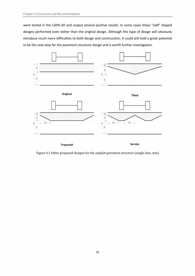
Chapter 6 Conclusions and Recommendations
92
were tested in the CAPA-3D and output several positive results. In some cases these “odd” shaped
designs performed even better than the original design. Although this type of design will obviously
introduce much more difficulties to both design and construction, it could still hold a great potential
to be the next step for the pavement structure design and is worth further investigation.
3050
80
1040
80
30
1020
50
80 400
1020
50
80 400 600
Figure 6.1 Other proposed designs for the asphalt pavement structure (single lane, mm)
Serrate
Original Tilted
Trapezoid

Bibliography
93
Bibliography
[1] Nikolaides, A.F. (2016). Sustainable and long life flexible pavements. Functional Pavement Design, 693–704.
[2] Hein, D. K., Rao, S., & Lee, H. (2016). Bases and Subbases for Concrete Pavements (No. FHWA-HIF-16-005).
[3] Jenkins, K. (2006). Introduction to Road Pavements. Hitchhiker’s Guide to Pavement Engineering, 1-11.
[4] Mathew, T. V. (2006). Transportation Engineering I. Mumbai, India: Civil Engineering–Transportation Engineering. IIT Bombay, NPTEL ONLINE.
[5] McNichol, D. (2005). Paving the way: asphalt in America. [6] South African National Roads Agency Limited. (2013). South African Pavement Engineering
Manual. [7] Christopher, B. R., Schwartz, C., & Boudreau, R. (2006). Geotechnical aspects of pavements:
Reference manual. US Department of Transportation, Federal Highway Administration. [8] Weingroff, R. F. (2016). Part 1: Essential to the National Interest. The Greatest Decade 1956-
1966: Celebrating the 50th Anniversary of the Eisenhower Interstate System. Federal Highway Administration, U.S. Department of Transportation.
[9] Lavin, P. (2003). Asphalt pavements: a practical guide to design, production and maintenance for engineers and architects. CRC Press.
[10] Pederson, N. J. (2007). Pavement Lessons Learned from the AASHO Road Test and Performance of the Interstate Highway System. Transport Research Board.
[11] American Association of State Highway, & Transportation Officials. (1993). AASHTO Guide for Design of Pavement Structures, 1993 (Vol. 1). AASHTO.
[12] Croney, D., & Croney, P. (1991). The design and performance of road pavements. [13] Robbins, M. M., Nam Tran, P. E., & Rodezno, C. (2014). Flexible Pavement Design–State of the
Practice NCAT Report 14-04. [14] Gemayel, C., & Maurovich, M. (2013). Mechanistic-Empirical Pavement Design. [15] Witczak, M. W., Andrei, D., & Houston, W. N. (2004). Guide for mechanistic-empirical design of
new and rehabilitated pavement structures. Transportation Research Board of the National Research Council, 1-91.
[16] Kim, M., Tutumluer, E., & Kwon, J. (2009). Nonlinear pavement foundation modeling for three-dimensional finite-element analysis of flexible pavements. International Journal of Geomechanics, 9(5), 195-208.
[17] AHMED, M. A., OTUOZE, H. S., & MURANA, A. A. (2011). Development of Finite Element Response Model for Mechanistic-Empirical Design of Flexible Pavement. Leonardo Electronic Journal of Practices and Technologies, (19), 69-84.
[18] Molenaar, A., Erkens, S., Huurman, R., Medani, T., & Visser, T. (2002). Characterisation and Modelling of Airfield Pavement Structures for Tomorrow’s Extra Large Aircraft. Federal Aviation Administration Airport Technology Transfer Conference. P-40.
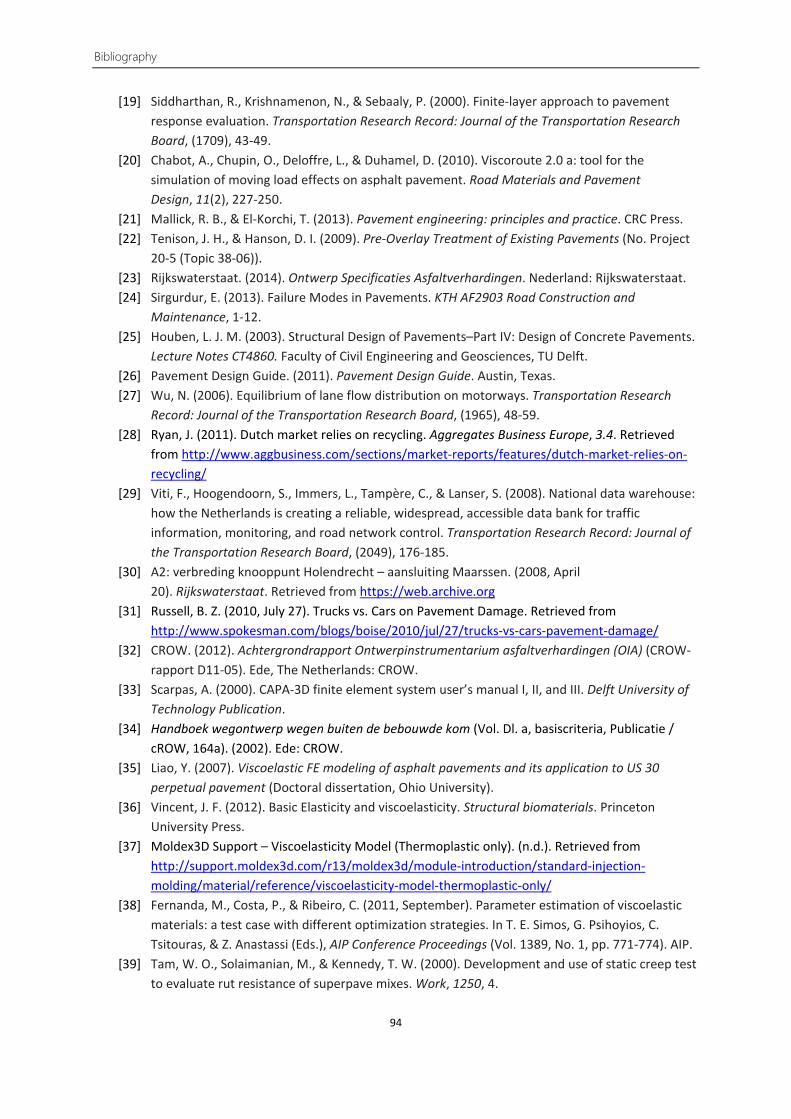
Bibliography
94
[19] Siddharthan, R., Krishnamenon, N., & Sebaaly, P. (2000). Finite-layer approach to pavement response evaluation. Transportation Research Record: Journal of the Transportation Research Board, (1709), 43-49.
[20] Chabot, A., Chupin, O., Deloffre, L., & Duhamel, D. (2010). Viscoroute 2.0 a: tool for the simulation of moving load effects on asphalt pavement. Road Materials and Pavement Design, 11(2), 227-250.
[21] Mallick, R. B., & El-Korchi, T. (2013). Pavement engineering: principles and practice. CRC Press. [22] Tenison, J. H., & Hanson, D. I. (2009). Pre-Overlay Treatment of Existing Pavements (No. Project
20-5 (Topic 38-06)). [23] Rijkswaterstaat. (2014). Ontwerp Specificaties Asfaltverhardingen. Nederland: Rijkswaterstaat. [24] Sirgurdur, E. (2013). Failure Modes in Pavements. KTH AF2903 Road Construction and
Maintenance, 1-12. [25] Houben, L. J. M. (2003). Structural Design of Pavements–Part IV: Design of Concrete Pavements.
Lecture Notes CT4860. Faculty of Civil Engineering and Geosciences, TU Delft. [26] Pavement Design Guide. (2011). Pavement Design Guide. Austin, Texas. [27] Wu, N. (2006). Equilibrium of lane flow distribution on motorways. Transportation Research
Record: Journal of the Transportation Research Board, (1965), 48-59. [28] Ryan, J. (2011). Dutch market relies on recycling. Aggregates Business Europe, 3.4. Retrieved
from http://www.aggbusiness.com/sections/market-reports/features/dutch-market-relies-on-recycling/
[29] Viti, F., Hoogendoorn, S., Immers, L., Tampère, C., & Lanser, S. (2008). National data warehouse: how the Netherlands is creating a reliable, widespread, accessible data bank for traffic information, monitoring, and road network control. Transportation Research Record: Journal of the Transportation Research Board, (2049), 176-185.
[30] A2: verbreding knooppunt Holendrecht – aansluiting Maarssen. (2008, April 20). Rijkswaterstaat. Retrieved from https://web.archive.org
[31] Russell, B. Z. (2010, July 27). Trucks vs. Cars on Pavement Damage. Retrieved from http://www.spokesman.com/blogs/boise/2010/jul/27/trucks-vs-cars-pavement-damage/
[32] CROW. (2012). Achtergrondrapport Ontwerpinstrumentarium asfaltverhardingen (OIA) (CROW-rapport D11-05). Ede, The Netherlands: CROW.
[33] Scarpas, A. (2000). CAPA-3D finite element system user’s manual I, II, and III. Delft University of Technology Publication.
[34] Handboek wegontwerp wegen buiten de bebouwde kom (Vol. Dl. a, basiscriteria, Publicatie / cROW, 164a). (2002). Ede: CROW.
[35] Liao, Y. (2007). Viscoelastic FE modeling of asphalt pavements and its application to US 30 perpetual pavement (Doctoral dissertation, Ohio University).
[36] Vincent, J. F. (2012). Basic Elasticity and viscoelasticity. Structural biomaterials. Princeton University Press.
[37] Moldex3D Support – Viscoelasticity Model (Thermoplastic only). (n.d.). Retrieved from http://support.moldex3d.com/r13/moldex3d/module-introduction/standard-injection-molding/material/reference/viscoelasticity-model-thermoplastic-only/
[38] Fernanda, M., Costa, P., & Ribeiro, C. (2011, September). Parameter estimation of viscoelastic materials: a test case with different optimization strategies. In T. E. Simos, G. Psihoyios, C. Tsitouras, & Z. Anastassi (Eds.), AIP Conference Proceedings (Vol. 1389, No. 1, pp. 771-774). AIP.
[39] Tam, W. O., Solaimanian, M., & Kennedy, T. W. (2000). Development and use of static creep test to evaluate rut resistance of superpave mixes. Work, 1250, 4.

Bibliography
95
[40] Perret, J., & Dumont, A. G. (2004). Strain and stress distributions in flexible pavements under moving loads. International Journal of Road Materials and Pavement Design, 5(LAVOC-ARTICLE-2004-001), 203-225.
[41] Hernandez, J., Al-Qadi, I., Ozer, H., Greene, J., Choubane, B., Wu, R., … Weaver, E. (2014). Pavement responses as function of truck tire type. Asphalt Pavements, 1125-1134. doi:10.1201/b17219-138
[42] Sebaaly, B. E., & Mamlouk, M. S. (1987). Prediction of pavement response to actual traffic loading.
[43] Pezo, R. F., Marshek, K. M., & Hudson, W. R. (1989). Truck tire pavement contact pressure distribution characteristics for the Bias Goodyear 18-22.5, the Radial Michelin 275/80R/24.5, the Radial Michelin 255/70R/22.5, and the Radial Goodyear 11R24. 5 tires (No. FHWA/TX-90+ 1190-2F). Center for Transportation Research, Bureau of Engineering Research, University of Texas at Austin.
[44] Priest, A. L., & Timm, D. H. (2006). Methodology and Calibration of Fatigue Transfer Functions for Mechanistic Empirical Flexible Pavement Design (NCAT Report 06-03).
[45] Al-Qadi, I. L., Loulizi, A., Elseifi, M., & Lahouar, S. (2004). The Virginia Smart Road: The impact of pavement instrumentation on understanding pavement performance. The Journal of Association of Asphalt Paving Technologists, 83, 427-66.
[46] Hjort, M., Haraldsson, M., & Jansen, J. M. (2008). Road Wear from Heavy Vehicles: An Overview. NVF Committee Vehicles and Transports, Nordiska vägtekniska förbundet.
[47] Laplace distribution - Wikipedia. (n.d.). Retrieved May 18, 2017, from https://en.wikipedia.org/wiki/Laplace_distribution
[48] Li, N. (2013). Asphalt Mixture Fatigue Testing: Influence of Test Type and Specimen Size (Doctoral dissertation, TU Delft, Delft University of Technology).
[49] Huang, W., Zhang, X., Rong, H., & Chen, B. (2015). Finite Element Method for predicting rutting depth of steel deck asphalt pavement based on Accelerated Pavement Test. Proceedings of the 3rd International Conference on Mechanical Engineering and Intelligent Systems (ICMEIS 2015). doi:10.2991/icmeis-15.2015.177
[50] Hallenbeck, M., Rice, M., Smith, B., Cornell-Martinez, C., & Wilkinson, J. (1997). Vehicle volume distributions by classification (No. FHWA-PL-97-025,).
[51] TG Road Safety. (2010). Safe distance between vehicles. Paris, France: Conference of European Directors of Roads.
[52] Witczak, M. W., & El-Basyouny, M. M. (2004). Appendix GG-1: Calibration of Permanent Deformation Models for Flexible Pavements. Guide for Mechanistic-Empirical Design of New and Rehabilitated Pavement Structures.
[53] Tseng, K. H., & Lytton, R. L. (1989). Prediction of permanent deformation in flexible pavement materials. In Implication of aggregates in the design, construction, and performance of flexible pavements. ASTM International.
[54] Pellenbarg, N. B. (1997). Groundwater amangement in the Netherlands: background and legislation. In ILRI workshop groundwater management (pp. 137-149).
[55] Rijkswaterstaat. (2016). European Truck Platooning Challenge 2016 - Lessons Learnt. Dutch Ministry of Infrastructure and the Environment.
[56] What is Truck Platooning? - EU Truck Platoon Challenge. (n.d.). Retrieved from https://www.eutruckplatooning.com/About/default.aspx
[57] Engineering and Regional Operations. (2017). Construction Manual (M 41-01.28). Washington State Department of Transportation.
Bibliography
96
[58] Caterpillar. (n.d.). New Equipment [Photograph]. Retrieved from http://www.cat.com/en_GB/products/new/equipment/
[59] Caterpillar. (2014). CAT® F-SERIES PAVERS AND SCREEDS (QEHQ1822 (10/14)). [60] Equipment Operator, Basic (NAVEDTRA 14081A). (2014). Naval Education and
Trainingprofessional Developmentand Technology Center. [61] Chartered Institution of Highways & Transportation (CIHT). (2012). Road Maintenance Review
International Comparison. World Road Association (WRA) UK. [62] Tjin-A-Tsoi, T. (Ed.). (2016). Transport and mobility. The Hague, The Netherlands: Statistics
Netherlands. [63] A2 motorway (Netherlands) - Wikipedia. (n.d.). Retrieved May 18, 2017, from
https://en.wikipedia.org/wiki/A2_motorway_(Netherlands) [64] Anp. (2016, February 4). [Photograph]. Retrieved from
http://www.volkskrant.nl/binnenland/vanaf-mei-s-avonds-130-per-uur-op-a2-tussen-utrecht-en-amsterdam~a4238231/
[65] Volvo. (2015). VOLVO FL [photograph]. Retrieved from http://www.volvotrucks.com/en-en/trucks/volvo-fl.html
[66] Rijkswaterstaat adviesdienst verkeer en vervoer. (2012). Atlas hoofdwegennet. Den Haag: Rijkswaterstaat.
[67] Alvarez, A. E., Mahmoud, E., Martin, A. E., Masad, E., & Estakhri, C. (2010). Stone-on-Stone Contact of Permeable Friction Course Mixtures. Journal of Materials in Civil Engineering, 22(11), 1129-1138. doi:10.1061/(asce)mt.1943-5533.0000117
[68] Van Haaster, B., Worrell, E., F. Fortuin, J. P., & Van Vliet, W. (2015). Potential Energy Savings by Reducing Rolling Resistance of Dutch Road Pavements. Journal of Materials in Civil Engineering, 27(1), 04014101. doi:10.1061/(asce)mt.1943-5533.0000999

Appendix
97
Appendix
Figure A.1 Typical vertical strain contour (2 passenger cars and 1 truck with dual tires)
Figure A.2 Typical transverse strain contour (broadband)
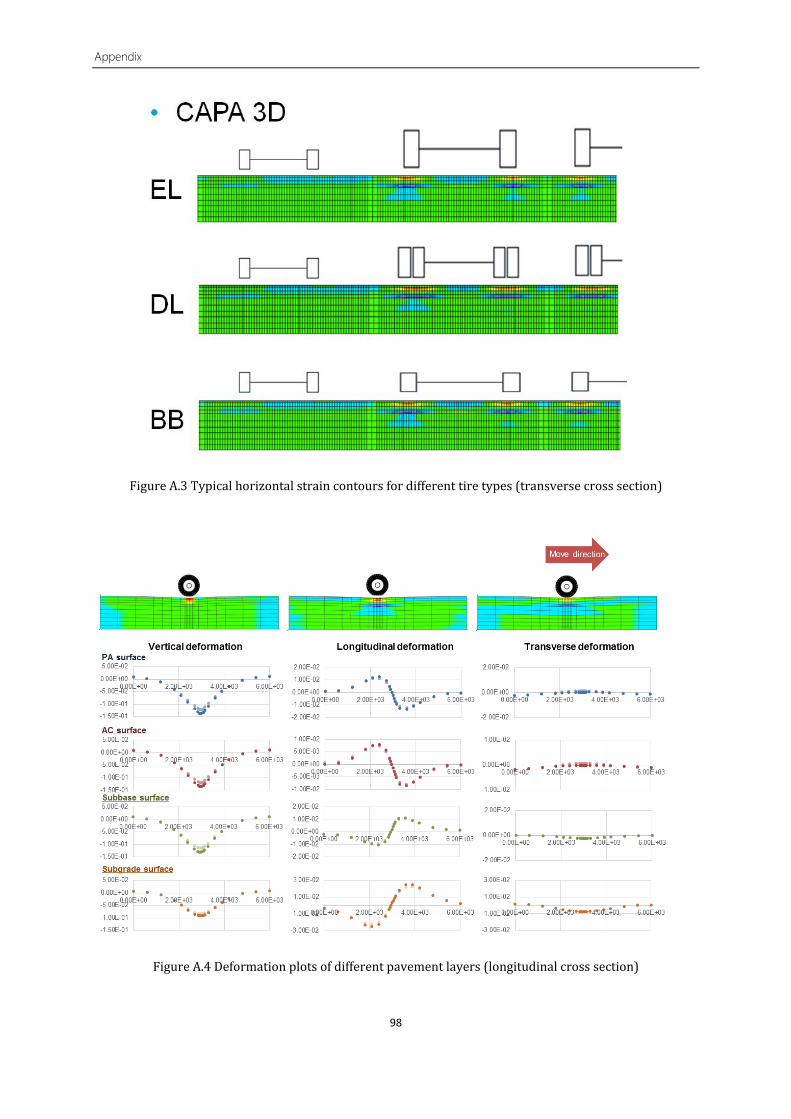
Appendix
98
Figure A.3 Typical horizontal strain contours for different tire types (transverse cross section)
Figure A.4 Deformation plots of different pavement layers (longitudinal cross section)
0

Appendix
99
Figure A.5 Vertical deformation plots of different pavement layers (transverse cross section)
Figure A.6 Longitudinal deformation plots of different pavement layers (transverse cross section)

Appendix
100
Figure A.7 Transverse deformation plots of different pavement layers (transverse cross section)
Figure A.8 Transverse deformation (absolute values) plots of different pavement layers (transverse cross section)


Author Name: Quanxin Xu
Student Number: 4308360
Mobile: (+31)(0)631556025
E-mail: [email protected]
University: Delft University of Technology
Faculty: Civil Engineering and Geosciences
Master Programme: Structural Engineering
Specialisation: Pavement Engineering