A POTENTIAL PANEL METHOD FOR THE PREDICTION OF MIDCHORD FACE AND BACK CAVITATION S. Gaggero & S. Brizzolara, University of Genoa (IT), Department of Naval Architecture and Marine Engineering SUMMARY Accurate predictions of the extent of thee sheet cavitation and the pressure distribution on the blade are crucial in the design and assessment of marine propulsor subjected to nonuniform unsteady flows. While, in normal operating conditions, cavitation occurs on the back side of the propeller and generally begins at the leading edge, when the propeller is subjected to a strong non axysymmetric flow cavitation can occur on the face side of the propeller. Moreover, at design advance coefficient, pressure distributions are often “flat” and this may lead to midchord or bubble cavitation. In the present work a three dimensional boundary element method is developed and validated for the prediction of general cavity patterns and loading, with convergence and consistency studies. First the method is validated against 3D cavitating wings in order to check the ability to search for simultaneous face and back cavitation with arbitrary detachment point and, after, the most general case of a propeller is analyzed in order to investigate about the performances of the developed method. 1. INTRODUCTION The design of modern marine propellers is more and more conditioned by the analysis of inception and developed cavitation. In recent years, the design of high speed marine vehicles has become increasing competitive together with a growing demand of heavily loaded propellers with request of very low noise and vibration levels onboard. Cavitation, thus, is the more important inhibitor to the propulsion system and it is comprehensive the need of a simple and fast method to predict cavitation behaviour of the propeller in the design stage. As known, cavitation under all its different configurations can generate a number of problems i.e. additional noise, vibrations and erosions, as well as, variations in the developed thrust and torque. The study of cavitation is very much complicated by the presence of a fluid with two different phases and the effect of viscosity is, in many cases, significant. Moreover, on modern propellers design, midchord cavitation and bubble cavitation may also appear and face cavitation is very common, specially if the propeller operates behind a strong nonuniform wake or in inclined shaft conditions. The most advance computational tools for cavitation analysis on marine propellers are based on RANS equations solvers. However unsteady cavitating RANS analysis are quite computationally expensive, so potential flow theory can be adopted for the preliminary analysis and design of cavitating propellers. At the University of Genova the development of a three dimensional boundary element method for the analysis of steady flow and steady cavitating flows was started by Caponnetto and Brizzolara [2]. Further developments have been made by Gaggero and Brizzolara [4], [5], with the inclusion of a wake alignment algorithm, an iterative

Kutta condition and an unsteady solver for fully wetted flows. In this work a panel method for the study of propellers subjected to cavitation is presented. The present method, first developed for the analysis of wings and after extended to treat the propeller problem, is limited to steady flow, adopts a sheet cavitation model and allows face and midchord cavitation. Since no universally accepted definition for midchord detachment exists, it can be defined as the detachment “well behind” the leading edge (Mueller and Kinnas [16]) and, although midchord cavitation often appears as cloud or bubble cavitation, in the framework of potential flow it can be treated again as sheet cavitation, because the attention is focused on global, mean and steady pressure distributions, for which the sheet cavitation model is enough. At this stage of development also supercavitation is neglected. In some critical conditions, midchord cavitation but also leading edge cavitation could lead to supercavitation for certain sections (in the propeller case those close to the tip). The present numerical method neglects the effect of sheet cavitation thickness in the wake and solves supercavitating sections leaving them open at trailing edge. In fact the influence of the sheet cavitation bubble in the wake on the solution (pressure distribution on the body) can be considered small enough to be not taken into account: in an ongoing research it has been proved that allowing for supercavitation alters only the sheet bubble development near the trailing edge (where the influence of the wake bubble is more significant), determining only a small variation of the cavitating bubble volume, but the general behaviour of the solution obtained neglecting supercavitation remains valid. The pressure distribution, with the typical constant value equal to the vapour pressure in the cavitating zones, is still valid and the inclusion of supercavitation

33

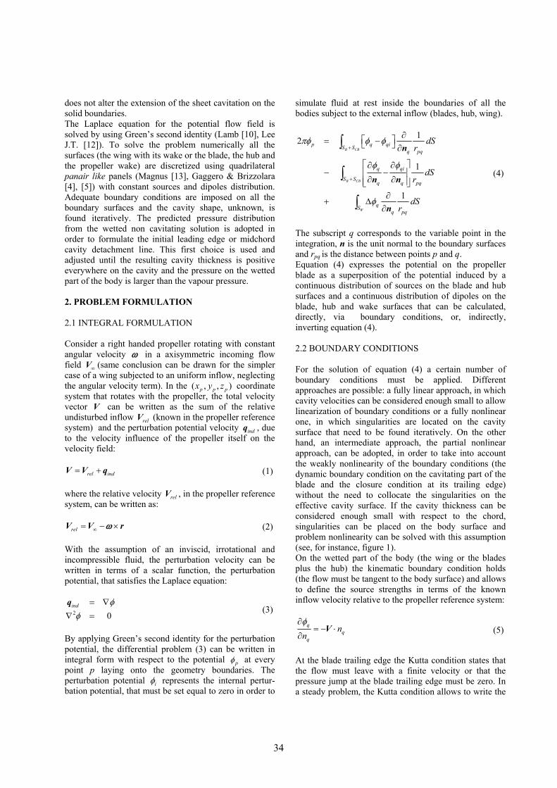
does not alter the extension of the sheet cavitation on the solid boundaries. The Laplace equation for the potential flow field is solved by using Green’s second identity (Lamb [10], Lee J.T. [12]). To solve the problem numerically all the surfaces (the wing with its wake or the blade, the hub and the propeller wake) are discretized using quadrilateral panair like panels (Magnus [13], Gaggero & Brizzolara [4], [5]) with constant sources and dipoles distribution. Adequate boundary conditions are imposed on all the boundary surfaces and the cavity shape, unknown, is found iteratively. The predicted pressure distribution from the wetted non cavitating solution is adopted in order to formulate the initial leading edge or midchord cavity detachment line. This first choice is used and adjusted until the resulting cavity thickness is positive everywhere on the cavity and the pressure on the wetted part of the body is larger than the vapour pressure. 2. PROBLEM FORMULATION 2.1 INTEGRAL FORMULATION Consider a right handed propeller rotating with constant angular velocity ω in a axisymmetric incoming flow field ∞V (same conclusion can be drawn for the simpler case of a wing subjected to an uniform inflow, neglecting the angular velocity term). In the ( , , )p p px y z coordinate system that rotates with the propeller, the total velocity vector V can be written as the sum of the relative undisturbed inflow relV (known in the propeller reference system) and the perturbation potential velocity indq , due to the velocity influence of the propeller itself on the velocity field:

rel ind= +V V q (1) where the relative velocity relV , in the propeller reference system, can be written as:

rel ∞= − ×ωV V r (2) With the assumption of an inviscid, irrotational and incompressible fluid, the perturbation velocity can be written in terms of a scalar function, the perturbation potential, that satisfies the Laplace equation:

2 0ind φφ

= ∇∇ =q

(3)

By applying Green’s second identity for the perturbation potential, the differential problem (3) can be written in integral form with respect to the potential pφ at every point p laying onto the geometry boundaries. The perturbation potential iφ represents the internal pertur-bation potential, that must be set equal to zero in order to

simulate fluid at rest inside the boundaries of all the bodies subject to the external inflow (blades, hub, wing).

12

1

1

B CB

B CB

W

p q qiS Sq pq

q qi

S Sq q pq

qSq pq

dSr

dSr

dSr

πφ φ φ

φ φ

φ

+

+

∂⎡ ⎤= −⎣ ⎦ ∂

⎡ ⎤∂ ∂− −⎢ ⎥

∂ ∂⎢ ⎥⎣ ⎦∂

+ Δ∂

∫

∫

∫

n

n n

n

(4)

The subscript q corresponds to the variable point in the integration, n is the unit normal to the boundary surfaces and rpq is the distance between points p and q. Equation (4) expresses the potential on the propeller blade as a superposition of the potential induced by a continuous distribution of sources on the blade and hub surfaces and a continuous distribution of dipoles on the blade, hub and wake surfaces that can be calculated, directly, via boundary conditions, or, indirectly, inverting equation (4). 2.2 BOUNDARY CONDITIONS For the solution of equation (4) a certain number of boundary conditions must be applied. Different approaches are possible: a fully linear approach, in which cavity velocities can be considered enough small to allow linearization of boundary conditions or a fully nonlinear one, in which singularities are located on the cavity surface that need to be found iteratively. On the other hand, an intermediate approach, the partial nonlinear approach, can be adopted, in order to take into account the weakly nonlinearity of the boundary conditions (the dynamic boundary condition on the cavitating part of the blade and the closure condition at its trailing edge) without the need to collocate the singularities on the effective cavity surface. If the cavity thickness can be considered enough small with respect to the chord, singularities can be placed on the body surface and problem nonlinearity can be solved with this assumption (see, for instance, figure 1). On the wetted part of the body (the wing or the blades plus the hub) the kinematic boundary condition holds (the flow must be tangent to the body surface) and allows to define the source strengths in terms of the known inflow velocity relative to the propeller reference system:

qq

q

nnφ∂

= − ⋅∂

V (5)

At the blade trailing edge the Kutta condition states that the flow must leave with a finite velocity or that the pressure jump at the blade trailing edge must be zero. In a steady problem, the Kutta condition allows to write the

34

dipole intensities, constant along each streamlines (equivalent to each chordwise strip in the discretized formulation), on the wake, first, applying the “linear” Morino Kutta condition:

. . . . . . . .U L

T E T E T E rel T Eφ φ φΔ = − + ⋅V r (6) where the sup scripts U and L stand for the upper and the lower face of the trailing edge. After, the zero pressure jump can be achieved via an iterative scheme. In fact the pressure difference at trailing edge (or the pressure coefficient difference) at each m streamlines (or at each m blade strip for the discretized problem) is a non linear function of dipole intensities on the blade:

( ) ( ) ( )U Lm m mp p pφ φ φΔ = − (7)

So, an iterative scheme is required to force a zero pressure jump, working on dipoles strength on the blade (and, consequently, on potential jump on the wake). By applying a Newton – Raphson scheme with respect to the potential jump on the wake φΔ , equal in the steady problem to the potential jump at blade trailing edge, the wake potential jump is given by:

{ } { } { }11 ( )k k kkJ pφ φ φ−+ ⎡ ⎤Δ = Δ − Δ⎣ ⎦ (8)

where the index k denotes the iteration, [ ]( ) kp φΔ is the pressure jump at trailing edge obtained solving the problem at iteration k (corresponding to the

kφΔ solution) and kJ⎡ ⎤⎣ ⎦ is the Jacobian matrix numerically determined (9):

kk iij k

j

pJ

φ∂Δ

=∂Δ

(9)

while, for the first iteration, the solution kφΔ and the corresponding pressure jump is taken from the linear Morino solution (6). Moreover the wake should be a streamsurface: the zero force condition is satisfied when the wake surface is aligned with the local velocity vector. In the present method this condition is only approximated and the wake surface is assumed frozen and laying on an helicoidal surface whose pitch is equal to the blade pitch. Assuming that the influence of the cavity bubble is small in the definition of the wake surface, an approach similar to that proposed by Gaggero & Brizzolara [4] can be adopted and the cavity solver could be improved using the aligned wake calculated for the steady non cavitating flow. Analogous (kinematic and dynamic) boundary conditions have to be forced on the body cavitating surfaces, in order to solve for the singularities (sources and dipoles)

distributed there (Caponnetto and Brizzolara [2], Fine [3], Mueller and Kinnas [16], Young and Kinnas [18], Vaz and Bosschers [17]). On the cavity surface SCB the pressure must be constant and equal to the vapour pressure or the modulus of the velocity, obtained via Bernoulli’s equation, must be equal to the total velocity VapV on the cavity surface.

Figure 1: Exact (SC) and approximate (SCB) cavity surface definition. If p∞ is the pressure of the undisturbed flow field, p is the actual pressure and ρ is the flow density, in a propeller fixed reference system, Bernoulli’s equation can be written in the following form:

2 2 21 12 2 shaftp p gyρ ρ∞ ∞

⎡ ⎤+ = + − × +⎣ ⎦V V rω (10)

If Vapp indicates the vapour pressure of the flow, the modulus of the corresponding vapour pressure VapV , via equation (10) on the cavity surface, along each section of constant radius, , is equal to:

( ) 2 22 2Vap Vap shaftp p gyρ ∞ ∞= − + + × −V V rω (11)

This dynamic boundary condition can be written as a Dirichlet boundary condition for the perturbation potential. In order to obtain a Dirichlet boundary condition from the dynamic boundary condition it is necessary, first, (following Brizzolara and Caponnetto [2]) to define the

35

controvariant components V α and the covariant components Vβ of the velocity vector V :

= V

V V V

αα

αβ β β α β= ⋅ → = ⋅

V e

V e e e (12)

where αe are the unit vector of the reference system and

,α β are equal to 1, 2 and 3. Defining the square matrix gαβ α β= ⋅e e and its inverse gαβ , the covariant component can be written as: V V g

V g V g g V

βα αβ

αγ β αγ γα αβ

=

= = (13)

Combining equations (12) with equations (13) the velocity vector V can be expressed in terms of the covariant components:

g Vαβα β=V e (14)

Figure 2: local non orthogonal panel coordinate system. Vectors l and m are formed by the lines connecting panel sides midpoints. Vector n is normal to l and m. In the present case (figure 2) the local coordinate system is defined by the vectors l, m and n, where cosθ⋅ =l m ,

= 0⋅l n and = 0⋅m n . The gαβ and the gαβ matrix can, thus, be written in the following form:

22

1 cos 0cos 1 0

0 0 1

1 cos 01 cos 1 0

sin0 0 sin

xy

xy

g

g

θθ

θθ

θθ

⎡ ⎤⎢ ⎥= ⎢ ⎥⎢ ⎥⎣ ⎦

−⎡ ⎤⎢ ⎥= −⎢ ⎥⎢ ⎥⎣ ⎦

(15)

while the expression of the gradient can be obtained, from (14) and (15), as:

22

1 cos 01 cos 1 0

sin0 0 sin

lmn

θθ

θθ

− ∂ ∂⎡ ⎤ ⎧ ⎫⎪ ⎪⎢ ⎥∇ = − ∂ ∂⎨ ⎬⎢ ⎥⎪ ⎪⎢ ⎥ ∂ ∂⎣ ⎦ ⎩ ⎭

(16)

The covariant component of the velocity on the non orthogonal reference system can be expressed as:

l rel l

m rel m

n rel n

V + Ul l

V + Um m

V + Un n

φ φ

φ φ

φ φ

∂ ∂= ⋅ = +

∂ ∂∂ ∂

= ⋅ = +∂ ∂∂ ∂

= ⋅ = +∂ ∂

V l

V m

V n

(17)

And, from equation (14) the velocity vector is given by:

( )

( )

2

2

1 cossin

1 cossin

l m

m l

n

V V

V V

V

θθ

θθ

⎛ ⎞= −⎜ ⎟⎝ ⎠⎛ ⎞+ −⎜ ⎟⎝ ⎠

V l

m

n

(18)

Assuming Vn vanishingly small, the normal component of the velocity can be neglected: in general it deteriorates the robustness of the solution and hardly influences the cavity extent as demonstrated by Fine [3]. Thus the modulus of the velocity becomes:

( )2 2 22

1 2 cossin l m l mV V g V V V Vβα

α β θθ

= = + −V (19)

Considering l approximately aligned with the local surface flow, it is possible to solve (19) with respect to

lφ∂ ∂ (because, from equation (17) l lV U lφ= + ∂ ∂ ) obtaining:

2

2

cos

sin

l m

m

U Ul m

Um

φ φ θ

φθ

∂ ∂⎛ ⎞= − + +⎜ ⎟∂ ∂⎝ ⎠

∂⎛ ⎞+ − +⎜ ⎟∂⎝ ⎠V

(20)

Equation (20) can be integrated to finally achieve a Dirichlet boundary condition for the perturbation potential, equivalent to the dynamic boundary condition. On the cavitating surface, where Vap=V V , equation (20), after integration between bubble leading edge and bubble trailing edge, yields to:

. .

0. .

22

( , ) ( ) cos

sin

Bub

Bub

T E

l mL E

Vap m

m l m U Um

U dlm

φφ φ θ

φθ

⎡ ∂⎛ ⎞= + − + +⎢ ⎜ ⎟∂⎝ ⎠⎣

⎤∂⎛ ⎞ ⎥+ − +⎜ ⎟∂ ⎥⎝ ⎠ ⎦

∫

V

(21)

36

where the only unknowns are the values of the perturbation potential at the bubble leading edge. The kinematic boundary condition on the cavity surface, in steady flow, requires the flow to be tangent to the cavity surface itself. With respect to the local (l,m,n) orthogonal coordinate reference system (figure 2), the cavity surface SC (in terms of its thickness t) is defined as:

( , ) ( , ) 0t - t= → =n l m n l m (22) and the tangency condition, by applying the covariant and the controvariant representation of velocity vectors and gradient defined above, can be written as:

( )( )( )

( , ) 0( , ) 0

( , ) 0

tV t

g V t

αα

αβα β

⋅∇ − =∇ − =∇ − =

V n l mn l m

n l m (23)

Moreover:

( )

( )

( )

( , )

( , )

( , ) 1

ttl l

ttm m

tn

∂ ∂− = −

∂ ∂∂ ∂

− = −∂ ∂∂

− =∂

n l m

n l m

n l m

(24)

And, from equation (16) and (23):

{ }2

2

1 , ,sin

1 cos 0cos 1 0 00 0 sin 1

l m nV V V

t lt m

θθ

θθ

⋅

− −∂ ∂⎡ ⎤ ⎧ ⎫⎪ ⎪⎢ ⎥− ⋅ −∂ ∂ =⎨ ⎬⎢ ⎥⎪ ⎪⎢ ⎥⎣ ⎦ ⎩ ⎭

(25)

Equation (25) yields to a differential equation for cavity thickness over the blade, with respect to the local reference system:

2

cos

cos

sin 0

m l

l m

n

t U Ul m l

t U Um l m

Un

φ φθ

φ φθ

φθ

⎡ ⎤∂ ∂ ∂⎛ ⎞ ⎛ ⎞+ − + +⎢ ⎥⎜ ⎟ ⎜ ⎟∂ ∂ ∂⎝ ⎠ ⎝ ⎠⎣ ⎦⎡ ⎤∂ ∂ ∂⎛ ⎞ ⎛ ⎞+ − + +⎢ ⎥⎜ ⎟ ⎜ ⎟∂ ∂ ∂⎝ ⎠ ⎝ ⎠⎣ ⎦

∂⎛ ⎞+ =⎜ ⎟∂⎝ ⎠

(26)

To solve for the cavity planform shape, another condition is required on the cavitating surface: the cavity height at its trailing edge must be zero (cavity closure condition).

This determines the necessity of an iterative solution to satisfy this, further, condition because the cavity height, computed via equation (26) is a non linear function of the solution (the perturbation potential φ ) and of the extent of the cavity surface (via the dynamic boundary condition):

. .( ) 0T Et l = (27) 2.3 MIDCHORD FACE AND BACK CAVITATION Midchord cavitation is becoming common in recent propeller designs: it is due to the attempt to increase efficiency, to the fact that, often, new design sections have flat pressure distributions on the suction side, or to the fact that a conventional propeller works in off design condition (Young and Kinnas [18 ], Mueller and Kinnas [16]). The non axisymmetric flow a propeller may experience inside a wake is, often, characterized by smaller incoming velocities at certain angular positions: this traduces in small or negative angles of attack that may lead to face cavitation. In order to capture simultaneously face and back cavitation and to allow midchord detachment, the theoretical formulation is exactly the same explained above with reference to the more common case of back cavitation only. The face cavitation problem can be treated exactly as the back cavitation problem, thus defining and adequate reference system (the face non orthogonal reference system needs to have the corresponding l unit vector pointing along the versus of the tangential velocity on the face of the profile) and imposing the same dynamic, kinematic and cavity closure conditions with respect to this, new, local reference system (figure 3).

Figure 3: Back and Face reference coordinate system. Arbitrary detachment line can be found, iteratively, applying criteria equivalent, in two dimensions, to the Villat-Brillouin cavity detachment condition (as in Young and Kinnas [18], Mueller and Kinnas [16]). Starting from a detachment line obtained from the initial wetted solution (and identified as the line that separates zones with pressures higher than the vapour tension from zones subjected to pressure equal or lower pressures) or an imposed one (typically the leading edge), the detachment line is iteratively moved according to:

37

• If the cavity at that position has negative thickness, the detachment location is moved toward the trailing edge of the blade.

• If the pressure at a position upstream the actual detachment line is below vapour pressure, then the detachment location is moved toward the leading edge of the blade.

3. NUMERICAL FORMULATION Equation (4) is a second kind Fredholm’s integral equation for the perturbation potential φ . Numerically it can be solved approximating boundary surfaces with quadrilateral panels, substituting integrals with discrete sums and imposing appropriate boundary conditions. The panel arrangement selected for this problem is the same adopted for the steady propeller panel method (Gaggero & Brizzolara [4], [5]), and, in discrete form, equation (4) takes the form:

1 1 1 1 1

1 1

1,

WNZ N Z Mz z z zij j iml ml

z j z m l

Z Nz zij j

z j

A W

B i N Z

μ φ

σ

= = = = =

= =

+ Δ =

= ×

∑∑ ∑∑∑

∑∑ (28)

where N is the number of panels on the body (the key blade and its hub in the case of the propeller, as in Gaggero & Brizzolara [5], or the wing), Z is the number of blades (zero in the case of the wing) and Aij, Bij, Wiml are the influence coefficients of the dipoles (unknowns) and the sources (knows from the kinematic boundary condition) on the body and of the dipoles (knows from the Kutta condition) on the wake. Equation (28) represents a linear algebraic system valid for the wetted problem: in the cavitating case, the kinematic boundary condition (equation (5)) holds only on the wetted part of the surface, while from the dynamical boundary condition on the cavitating surface, the dipoles intensity (except for the dipoles intensity at bubble detachment) is known (equation (21)). Thus linear system (28) can be rewritten taking into account the boundary conditions on the cavitating surfaces. From the dynamic boundary condition (21), numerically solved via a quadrature technique, the dipoles intensity on each cavitating i panel of the j cavitating strip can be written as:

.

.

. .

0. .

Bub

Bub

T E

ij j iji L E

Fφ φ=

= + ∑ (29)

in which 0 jφ is the perturbation potential, unknown, at the cavitation bubble leading edge for the j strip and ijF is the numerical values of the integral in equation (21).

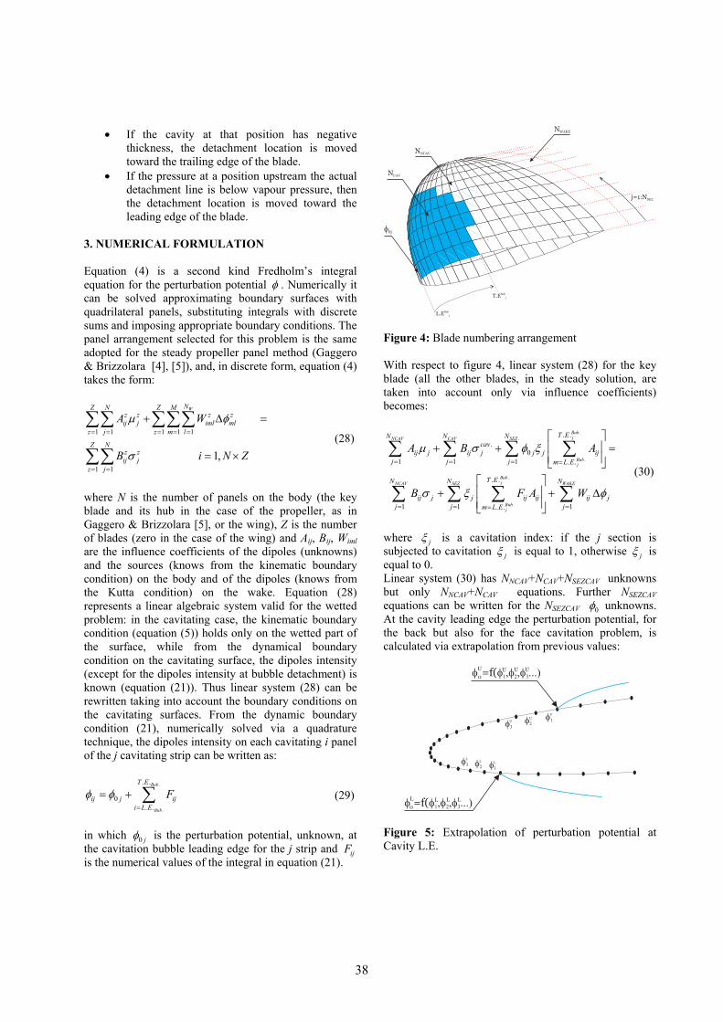
Figure 4: Blade numbering arrangement With respect to figure 4, linear system (28) for the key blade (all the other blades, in the steady solution, are taken into account only via influence coefficients) becomes:

..

.

..

.

. ..

01 1 1 . .

. .

1 1 1. .

BubjNCAV CAV SEZ

Bubj

BubjNCAV SEZ WAKE

Bubj

T EN N Ncav

ij j ij j j j ijj j j m L E

T EN N N

ij j j ij ij ij jj j jm L E

A B A

B F A W

μ σ φ ξ

σ ξ φ

= = = =

= = ==

⎡ ⎤⎢ ⎥+ + =⎢ ⎥⎣ ⎦

⎡ ⎤⎢ ⎥+ + Δ⎢ ⎥⎣ ⎦

∑ ∑ ∑ ∑

∑ ∑ ∑ ∑ (30)

where jξ is a cavitation index: if the j section is subjected to cavitation jξ is equal to 1, otherwise jξ is equal to 0. Linear system (30) has NNCAV+NCAV+NSEZCAV unknowns but only NNCAV+NCAV equations. Further NSEZCAV equations can be written for the NSEZCAV 0φ unknowns. At the cavity leading edge the perturbation potential, for the back but also for the face cavitation problem, is calculated via extrapolation from previous values:

Figure 5: Extrapolation of perturbation potential at Cavity L.E.

38

( )( )

0 1 2 3

0 1 2 3

, , ,...

, , ,...

U U U U

L L L L

f

f

φ φ φ φ

φ φ φ φ

=

= (31)

Once the problem has been solved for a guessed cavity planform and the perturbation potential and the cavity source strengths are knowns, the cavity height on the blade can be computed by integrating equation (26). Replacing the partial derivatives with finite difference formulae, it is possible to obtain a recursive expression for the cavity thickness at a point (l,m) as a function of cavity thickness on previous computed ones (l-1, m-1):

, 1, , , 1 0l m l m l m l mL M N

t t t tK K K

l m− −− −⎛ ⎞ ⎛ ⎞

+ + =⎜ ⎟ ⎜ ⎟Δ Δ⎝ ⎠ ⎝ ⎠ (32)

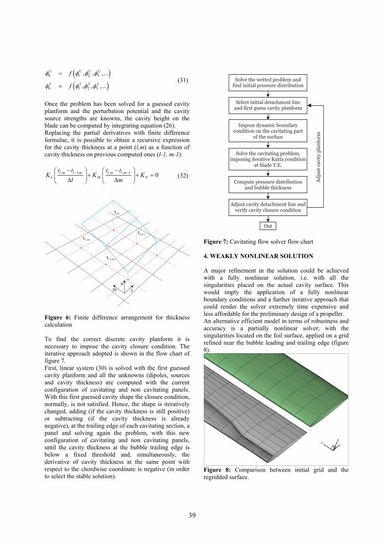
Figure 6: Finite difference arrangement for thickness calculation To find the correct discrete cavity planform it is necessary to impose the cavity closure condition. The iterative approach adopted is shown in the flow chart of figure 7. First, linear system (30) is solved with the first guessed cavity planform and all the unknowns (dipoles, sources and cavity thickness) are computed with the current configuration of cavitating and non cavitating panels. With this first guessed cavity shape the closure condition, normally, is not satisfied. Hence, the shape is iteratively changed, adding (if the cavity thickness is still positive) or subtracting (if the cavity thickness is already negative), at the trailing edge of each cavitating section, a panel and solving again the problem, with this new configuration of cavitating and non cavitating panels, until the cavity thickness at the bubble trailing edge is below a fixed threshold and, simultaneously, the derivative of cavity thickness at the same point with respect to the chordwise coordinate is negative (in order to select the stable solution).

Figure 7: Cavitating flow solver flow chart 4. WEAKLY NONLINEAR SOLUTION A major refinement in the solution could be achieved with a fully nonlinear solution, i.e. with all the singularities placed on the actual cavity surface. This would imply the application of a fully nonlinear boundary conditions and a further iterative approach that could render the solver extremely time expensive and less affordable for the preliminary design of a propeller. An alternative efficient model in terms of robustness and accuracy is a partially nonlinear solver, with the singularities located on the foil surface, applied on a grid refined near the bubble leading and trailing edge (figure 8).

XY

Z

Figure 8: Comparison between initial grid and the regridded surface.

39

Also in this case, the best solution arises from an iterative approach, as presented in the flow chart of figure 9. After the first partial nonlinear cavity solution on the initial grid, surfaces are regridded in order to cluster panels near leading and trailing cavity bubble edge. Then the problem is solved until a converged solution is achieved.

Figure 9: Partial nonlinear solver flow chart

However, regridding and recomputing influence coefficients at each iteration is quite time expensive. Thus, this partial nonlinear approach with regridding is useful to validate the implemented 3D solver: after convergence, the blade surface can be moved according to the computed cavity thickness and the so changed geometry adopted for a “fully wetted solution”.

Figure 10: Deformed surface configuration

The fully wetted solution is a measure of the consistency of the cavitating solution. The sheet bubble cavitation has been computed, via the kinematic boundary condition, as a streamline for the flow, imposing that the total velocity on that streamline is equivalent to the vapour pressure. So, the wetted solution, computed on the deformed geometry, should shows a flat pressure distribution, equal to the vapour pressure, over all the computed cavitating area of the blade.

Figure 11: Consistency test, NACA0015 wing, α = 5°, y/s = 0 Figures 11 and 12 show the comparison between the fully wetted solution, computed on the deformed geometry obtained on the regridded surface, and the partial nonlinear solution without regridding. It is clear how the two solutions are in good mutual agreement: the fully wetted solution on the deformed geometry captures well the behaviour of pressure at the bubble leading and trailing edge and shows the typical flat vapour pressure zone.

Figure 12: Consistency test, NACA0015 wing, α = 5°, y/s = 0.54

40

On the other hand, the partial nonlinear solution without regridding, with an adequate chordwise number of panels, ensures a sufficiently good solution, with a much greater computational efficiency. 5. NUMERICAL RESULTS 5.1 CONVERGENCE To test the numerical cavitating flow solver, a convergence and consistency analysis based on three dimensional wings has been carried out, in order to check about the stability and the robustness of the code. Unfortunately, it is quite difficult to find in literature a systematic study on cavitating wings: there are only few numerical results, while experimental data are, essentially, in terms of sketches or pictures of the cavity pattern recognized at the cavitation tunnel. Thus, to validate the solver, a rectangular wing, NACA 0006 profile, with aspect ratio equal to 4, operating at a cavitation index 2( ) (0.5 )V Vapp p Vσ ρ= − equal to 0.6 has been tested since, for this configuration, other numerical solutions are available (Bal & Kinnas [1]). Figure 13 shows the behaviour of the solution, in term of developed cavity bubble, with the number of panels along the chord: this seems to be the most important parameter for the convergence, because of the assumption, in the dynamic boundary condition, that the velocity is almost aligned with the local l vector. With respect to the fully wetted solver (Gaggero and Brizzolara [4]), the convergence is sensitively slower and an acceptable solution is achieved with a number of panel along the profile greater than seventy. In particular, the solution is affected by the number of panels at the trailing edge of the bubble, where the relative dimension of the panels is greater (due to the full cosine spacing that clusters point near the blade leading and trailing edge) and this influence the value of the dynamic boundary condition integral.

−0.4 −0.3 −0.2 −0.1 0 0.1 0.2 0.3 0.4−0.1

−0.05

0

0.05

0.1

0.15

0.2

x/c

20x4020x5020x6020x7020x8020x90NACA0006

Figure 13: Convergence analysis, NACA 0006 profile, α=4°, σV=0.6 at midspan. For this configuration other numerical results are available. Bal & Kinnas [1] performed a calculation with the code developed, for the first time, at M.I.T. by Fine [3], on the same rectangular wing. Their results, and a comparison with those from the present method, are reported in figure 14.

−0.4 −0.3 −0.2 −0.1 0 0.1 0.2 0.3 0.4−0.1

−0.05

0

0.05

0.1

0.15

0.2

x/c

present methodNACA0006Bal & Kinnas

Figure 14: Comparison between preset method and results from Bal & Kinnas, NACA 0006 profile, α=4°, σV=0.6 at midspan. The comparison between the present method and Bal & Kinnas shows an overall good agreement of the computed thickness on the midspan section. Only a little difference persists at cavity trailing edge: Bal & Kinnas predict a cavity planform slightly longer than that predicted by the present method.

Figure 15: Cavity thickness distribution, NACA 0006 profile, α=4°, σV=0.6. This difference can be attributed to a different cavity closure condition and to a different panel arrangement. Bal & Kinnas computation are performed using the so called “panel split technique” (Fine [3]) in order to reduce the influence of panels partially subjected to the cavity and partially subjected to the wetted flow on the stability of the solution. Their PROPCAV code find a continuous cavity planform iteratively using a cavity closure condition on the curvilinear coordinate along the profile, while present method works only in a discrete way, adding or subtracting an entire panel at the cavity trailing edge. Moreover they apply a grid refinement at the cavity trailing edge to reduce the error in the computation of the dynamic condition integral.

5.2 BACK AND FACE CAVITATION Also for the case of face and back simultaneous cavitation, with arbitrary detachment line, no experimental data were available for validation. Only a numerical validation of the code (consistency and convergence) has been done therefore.

41

Figure 16: Pressure distribution based on the fully wetted solution. Figure 16 shows the pressure distribution at midspan for a rectangular wing with NACA66 profile, a08 camber line, thickness over chord ratio equal to 0.1, camber over chord ratio equal to 0.06, tested with a negative angle of attack (α = -3°), at a velocity of 20 m/s (σV = 0.52). The pressure distribution is obtained in the fully wetted condition, i.e. without taking into account the risk of cavitation and its effects on the pressure distribution. Working with a negative angle of attack determines an inversion in the pressure distribution at blade leading edge: the pressure side (face of the wing) is subjected to a pressure greatly lower than the vapour pressure, while the suction side (back of the wing) experiments such lower values of pressure only from midchord position. So, it is clear the necessity of a code able to predict, simultaneously, face, back and midchord cavitation, in order to capture the effects of the cavity bubble on the pressure distribution (and, so, on the performance of the wing/propeller) also in off-design working conditions. Figure 17 shows the pressure distribution obtained with the cavity solver and compares it with the fully wetted solution. Three main aspects of the solution can be highlighted. First, face and back cavitation, with midchord detachment, is simultaneously well captured: it appears as a constant pressure distribution, equal to the vapour pressure, on all the areas subjected to the sheet cavity bubble. Secondly, from pressure diagram, the effect of the developed cavity can be outlined: the constant vapour pressure affects a length greater than that identified by the fully wetted solution, i.e. that area subjected to a pressure lower than the vapour tension. This is due to the fact that the cavity bubble detaches from the first point having pressure lower than vapour tension, but its length can overcome the chordwise extension of the lower pressure region found by the fully wetted solver.

Figure 17: Pressure distribution based on the cavity solution. The extension of the cavity bubble arises from the kinematic boundary condition and from the cavity closure condition, that impose the vapour pressure on all the length of the converged cavity bubble. Finally, it can be noted that the iterative Kutta condition is able, also in the case of cavitating flows, to guarantee closed pressure diagrams at blade trailing edge, even if the profile is supercavitating and the cavity bubble has a finite thickness at its trailing edge. Figure 18, instead, shows, for the same wing, the cavity shape at midspan. A smooth detachment, according to the Villat-Brillouin cavity detachment criteria is evident, either in the case of face leading edge detachment and in the case of midchord back detachment. Figures 19 and 20 show a typical prediction of cavitation pattern obtained with the code using the previously detailed hydrofoil geometry. The blade is tested at positive and negative angles of attack (±9°), with a cavitation index σV equal to 1.47.

−0.5 −0.4 −0.3 −0.2 −0.1 0 0.1 0.2 0.3 0.4 0.5

−0.2

−0.1

0

0.1

0.2

0.3

x/c Figure 18: Cavity shape at midspan based on cavity solution.

42

Results show the ability of the code to detect back and face leading edge cavitation and to predict the correct pressure distribution on it (figure 21 and 22).

Figure 19: Cavity planform, NACA66 a08 hydrofoil, α = 9°, σV = 1.47

Figure 20: Cavity planform, NACA66 a08 hydrofoil, α = - 9°, σV=1.47

−0.5 −0.4 −0.3 −0.2 −0.1 0 0.1 0.2 0.3 0.4 0.5−1

−0.5

0

0.5

1

1.5

2

2.5

x/c

−C

P

C

P wetted

CP Cav. Flow

Figure 21: Pressure distribution at midspan, NACA66 a08 hydrofoil, α = 9°, σV = 1.47 (wetted solution versus cavitating solution). Finally figures 23 and 24 present a numerical validation of the code in case of simultaneous face and back cavitation. The test is performed by comparing the cavity shape of the same hydrofoil, once with positive camber and positive angle of attack, and the once with inverted (negative) camber and negative angle of attack.

−0.5 −0.4 −0.3 −0.2 −0.1 0 0.1 0.2 0.3 0.4 0.5−1

0

1

2

3

4

5

6

7

x/c

−C

P

C

P wettedC

P Cav. Flow

Figure 22: Pressure distribution at midspan, NACA66 a08 hydrofoil, α = -9°, σV = 1.47 (wetted solution versus cavitating solution).

XY

Z

Figure 23: Validation of simultaneous face and back cavitation on an asymmetric rectangular hydrofoil, NACA 66 a08, α = +3° .

XY

Z

Figure 24: Validation of simultaneous face and back cavitation on an asymmetric rectangular hydrofoil, NACA 66 a08, α = -3° . As expected, the symmetry of the solution with respect to the x-y plane, is verified by the two calculation cases. Moreover a nice and smooth detachment for the back midchord bubble and for the leading edge face bubble is verified.

43

6. THE PROPELLER PROBLEM The cavitating propeller problem represents the main scope of application for the devised potential panel method: predict the correct cavity extent on back and face sides is fundamental to calculate hydrodynamic forces, obtained via integration of pressure on the blade, for particular or off design operating conditions. As in the case of hydrofoils (figure 21 and 22), integrating the wetted pressure distribution or the cavitating flow pressure distribution would lead to very different global values.

Figure 25: Propeller DTMB 4148, back cavitation, J = 0.6, σN = 1.5 As an example, the results obtained in the case of DTMB 4148 propeller are presented. The 4148 is a three blade propeller, adopted for a wide range of experimental measurements and numerical calculations, specially to test unsteady cavitation (Mueller and Kinnas [16], Young and Kinnas [18]). Figure 25 shows the cavity shape for the propeller working at an off design advance coefficient J = 0.6, with cavitation index 2 2( ) (0.5 )N Vapp p D Nσ ρ= − equal to 1.5. The panelling arrangement is done with 20 sections along the radius and 70 panels along the chord, in order to obtain a satisfying solution, in terms of convergence and robustness, in a reasonable calculation time. With this parameters choice, the cavity bubble develops only on the back side of the propeller and it detaches, mostly, at blade leading edge or just 2÷3 % aft the leading edge. In extreme working conditions (different J or σ) the propeller goes into a face and midchord cavitation. As presented in figures 26 and 27, with a greater advance coefficient (that induces negative angles of attack) and a lower value of cavitation index (σΝ 0.9), the propeller is

subjected to a face super-cavitation that starts from the leading edge (the cavity thickness is finite along almost all the blade trailing edge, as it is possible to see from figure 27).

Figure 26: Propeller DTMB 4148, back cavitation, J = 1.1, σN = 0.9

Figure 27: Propeller DTMB 4148, face cavitation, J = 1.1, σN = 0.9 On the back side, simultaneously, midchord cavitation occurs (figure 26) with a thinner bubble extended up to the blade trailing edge. For validation of the cavitating propeller case a set of experimental tests carried out at the cavitation tunnel of the Department of Naval Architecture of the University of Genova, have been selected. The propeller model E033 is a four bladed propeller, having a diameter of

44

0.227m, with moderate rake and skew distribution and a base NACA16 profile.

Figure 28: Propeller E033, J = 0.9, σN = 3.5, back pressure distribution

Figure 29: Propeller E033, J = 0.9, σN = 3.5, face pressure distribution

While it is quite difficult to directly measure pressure on the blade surface (so figures 28 and 29 report only computed pressure coefficient), a simple comparison between experiments and the numerical code can be carried out with respect to cavity extent. Figures 30 and 31 show the predicted (left) and the real (right) cavity extent for the E033 propeller, tested at two different advance coefficients and at two different cavitation indexes.

Figure 30: Propeller E033, J = 0.9, σN = 3.5 The propeller, in steady flow, is subjected only to back cavitation (observed during experiments and numerically computed), with a quite strong tip vortex cavitation, that the present method is still not able to predict. However, a satisfying prediction of the cavitation pattern on the blade is found.

Figure 31: Propeller E033, J = 0.8, σN = 2.5 7. CONCLUSION Theoretical and numerical details of a stationary potential flow panel method able to predict face and back cavitation on three dimensional lifting bodies, such as hydrofoils and propellers, have been presented in the paper. The method relies on a robust and generalized numerical scheme which allows the detachment of the bubble from multiple and sparse points on the modeled surfaces. Several application examples given in the paper demonstrate this ability of the code. The good

45

consistency of the partially non-linear model used to solve boundary conditions on the cavities, has been verified against a fully wetted model applied on the deformed hydrofoil surface with the previously computed cavity shape. The accuracy and convergence of the method have been presented and discussed in the case of cavitating three dimensional hydrofoils, showing good correlation with similar numerical simulations. The application of the method, in case of a propeller evidenced excellent correlation with experimental results in terms of predicted cavity planform shape. Further developments of the presented method currently planned are the extension of the method to deal with non-stationary flows and the possibility to predict and solve super-cavitating bubbles. 8. REFERENCES 1. BAL S. and KINNAS S.A. ‘A BEM for the Prediction of Free Surface Effects on Cavitating Hydrofoils’. Computational Mechanics (28), 2002. 2. CAPONNETTO M. and BRIZZOLARA S. ‘ Theory and Experimental Validation of a Surface Panel Method for the Analysis of Cavitating Propellers in Steady Flow’. PROPCAV ’95 Conference, Newcastle Upon Tyne, U.K., 1995. 3. FINE N.E. ‘Nonlinear Analysis of Cavitating Propellers in Nonuniform Flow’. Ph.D Thesis, M.I.T. Department of Ocean Engineering, 1992. 4. GAGGERO S. and BRIZZOLARA S. ‘Exact Modelling of Trailing Vorticity in Panel Methods for Marine Propeller’. 2nd International Conference on Marine Research and Transportation, Ischia, 2007. 5. GAGGERO S and BRIZZOLARA S. ‘A Potential Panle Method for the Analysis of Propellers in Unsteady Flow’. 8th Symposium on High Speed Marine Vehicles, Naples, 2008. 6. HOSHINO T. ‘Hydrodynamic Analysis of Propeller in Unsteady Flow Using a Surface Panel Method’, Journal of the Society of Naval Architects of Japan, Vol. 174, pp 71-87, 1993.

7. HOSHINO T. ‘Numerical and Experimental Analysis of Propeller Wake by Using a Surface Panel Method and a 3-Component LDV’, 18th Symposium on Naval Hydrodynamics, 1991. 8. HSIN C.H. ‘Development and Analysis of Panel Methods for Propeller in Unsteady Flow’. Ph.D Thesis, M.I.T. Department of Ocean Engineering, 1990. 9. JESSUP S. ‘An Experimental Investigation of Viscous Effects of Propeller Blade Flow’. Ph.D Thesis, The Catholic University of America, 1989. 10. LAMB H. ‘Hydrodynamics’. Cambridge University Press, 1932. 11. LEE H. ‘Modelling of Unsteady Wake Alignment and Developed Tip Cavitation’. Ph.D Thesis, The Environmental and Water Resource Engineering Department of Civil Engineering, The University of Texas at Austin, 2002. 12. LEE J.T. ‘A Potential Based Panel Method for the Analysis of Marine Propeller in Steady Flow’. Ph.D Thesis, M.I.T. Department of Ocean Engineering, 1987. 13. MAGNUS A.E. and EPTON M.A. ‘PAN AIR-A Computer Program for Predicting Subsonic or Supersonic Linear Potential Flows About Arbitrary Configurations Using A Higher Order Panel Method’, Vol. 1. Theory Document (Version 1.0), NASA CR-3251, 1980. 14. MASKEW B. ‘VSAERO Theory Document’. NASA Ames Research Center, 1984. 15. MORINO L. and KUO C.C. ‘Subsonic potential aerodynamic for complex configurations: a general theory’. AIAA Journal, Vol. 12, 1974. 16.MUELLER A.C. and KINNAS S.A. ‘Propeller Sheet Cavitation Predictions Using a Panel Method’. Journal of Fluids engineering, vol. 121, 1999. 17. VAZ G. and BOSSCHERS J. ‘Modelling Three Dimensional Sheet Cavitation on Marine Propellers Using a Boundary Element Method’. 6th International Symposium on Cavitation, The Netherlands, 2006. 18. YOUNG Y.L. and KINNAS S.A. ‘ A BEM for the Prediction of Unsteady Midchord Face and/or Back Propeller Cavitation’. Journal of Fluids Engineering, vol. 123, 2001.

46