A Practical Approach to Morse-Smale Complex Computation:Scalability and Generality

Attila Gyulassy, Peer-Timo Bremer, Member, IEEE, Bernd Hamann, Member, IEEE, and Valerio Pascucci, Member, IEEE

Abstract—The Morse-Smale (MS) complex has proven to be a useful tool in extracting and visualizing features from scalar-valueddata. However, efficient computation of the MS complex for large scale data remains a challenging problem. We describe a newalgorithm and easily extensible framework for computing MS complexes for large scale data of any dimension where scalar valuesare given at the vertices of a closure-finite and weak topology (CW) complex, therefore enabling computation on a wide variety ofmeshes such as regular grids, simplicial meshes, and adaptive multiresolution (AMR) meshes. A new divide-and-conquer strategyallows for memory-efficient computation of the MS complex and simplification on-the-fly to control the size of the output. In additionto being able to handle various data formats, the framework supports implementation-specific optimizations, for example, for regulardata. We present the complete characterization of critical point cancellations in all dimensions. This technique enables the topologybased analysis of large data on off-the-shelf computers. In particular we demonstrate the first full computation of the MS complex fora 1 billion/10243 node grid on a laptop computer with 2Gb memory.

Index Terms—Topology-based analysis, Morse-Smale complex, large scale data.

1 INTRODUCTION

Scientific data is becoming increasingly complex, and sophisticatedtechniques are required for its effective analysis and visualization. Ad-ditionally, data size increases accordingly with the size of memory,therefore analysis techniques must also be scalable. Topology-basedvisualization has become a useful technique in extracting features for awide range applications, primarily due to its ability to simplify featuresin a controlled manner. The MS complex is a structure that representsthe gradient flow behavior and completely encapsulates the topologyof level sets of a scalar function. It has been shown to be effective inidentifying, ordering, and selectively removing features. Computinga combinatorially correct MS complex is very challenging, and previ-ous algorithms are memory-intensive and computationally expensive,restricting their use to smaller datasets.

We present a new algorithm for constructing a consistent MS com-plex: a framework which utilizes a divide-and-conquer strategy fordealing with large scale data in a variety of data formats and of anydimension. The kernel of our algorithm computes the discrete gradi-ent on a parcel of the input data, generates an MS complex from thegradient on the parcel, and then merges the MS complexes togetheracross the boundaries of the parcels. We use the discrete formulationof Morse theory as opposed to the continuous formulation for two rea-sons: it is simpler to implement because there are no special caseswhen dealing with higher dimensional components of the MS com-plex; and it makes it possible to fix the gradient flow on the boundaryof parcels to enable a stratified approach. The discrete gradient andMS complex are computed independently on each parcel, and only theMS complex and gradient on the boundary of the parcel are necessaryto merge parcels. We can control the size of the parcels and size ofthe MS complex through simplification to obtain a memory-efficientalgorithm. We resolve degeneracies in the scalar function, such as flatregions and multi-saddles, in a consistent manner and construct the

• Attila Gyulassy is with UC Davis and Lawrence Livermore NationalLaboratory, E-mail: aggyulassy@ucdavis.edu.

• Peer-Timo Bremer is with Lawrence Livermore National Laboratory,E-mail: ptbremer@acm.org.

• Bernd Hamann is with University of California, Davis, E-mail:hamann@cs.ucdavis.edu.

• Valerio Pascucci is with University of Utah, E-mail: pascucci@acm.org.

Manuscript received 31 March 2008; accepted 1 August 2008; posted online19 October 2008; mailed on 13 October 2008.For information on obtaining reprints of this article, please sende-mailto:tvcg@computer.org.

discrete gradient field and associated MS complex to agree with thescalar flow wherever possible. We characterize cancellation operationsfor MS complexes of any dimensions. We present the algorithm in aframework that makes it possible to implement multiple data formatsby means of simple query functions, and also permits format-specificoptimizations, for example, for regular grids. We show that this ap-proach is comparable in performance to the fastest previous algorithm,but applicable to significantly larger data sets.

1.1 Related workOften, features in a scalar field correspond to topological changes inthe isosurface during a sweep of the domain. The life-cycle of atopological feature during this sweep is indicated by a pair of criti-cal points, one indicating the creation of the feature and the other thefeature’s destruction. Topology-aware methods have proven to be ef-fective in controlled simplification of scalar functions and hence inthe creation of multiresolution representations. As opposed to geome-try simplification using mesh decimation operators like edge contrac-tion [7, 11, 12, 18, 23, 30], which result in unpredictable simplifica-tion of topological features, topology-aware methods either monitorchanges to the topology [6, 13] or explicitly compute the topologicalfeatures and perform necessary geometric operations to remove smallfeatures.

The Reeb graph [26] traces components of isosurfaces (or contours)as one sweeps through the allowed range of isovalues. In the caseof simply connected domains, the Reeb graph has no cycles and iscalled a contour tree. Reeb graphs, contour trees, and their variantshave been used successfully to guide the removal of topological fea-tures [7, 4, 14, 31, 32, 33, 3]. Of particular note is the approach byPascucci et al. [24], which shows how the Reeb graph can be con-structed in a streaming manner for large datasets. Reeb graphs andcontour trees have been used to trace the construction, merging, anddestruction of isosurface components. The MS complex, however, isa more complete description, since it also detects genus changes inisosurfaces.

Partitions of surfaces induced by a piecewise-linear function havebeen studied in different fields, under different names, motivated bythe need for an efficient data structure to store surface features. Cay-ley [5] and Maxwell [22] proposed a subdivision of surfaces usingpeaks, pits, and saddles along with curves between them. The develop-ment of various data structures for representing topographical featureswas discussed by Rana [25].

The MS complex is a topological data structure that providesan abstract representation of the gradient flow behavior of a scalarfield [29, 28]. Edelsbrunner et al. [9] defined the MS complex for

piecewise-linear 2-manifolds by considering the PL function as thelimit of a series of smooth functions and used this intuition to transferideas from the smooth case. They also provided an efficient algorithmto compute the MS complex, restricted to edges of the input triangula-tion, and to build a hierarchical representation by repeated cancellationof pairs of critical points.

Bremer et al. [2] improved on the algorithm and described a multi-resolution representation of the scalar field. Both algorithms tracepaths of steepest ascent and descent beginning at saddle points. Thesepaths constitute boundaries of 2D cells of the MS complex. Cells inthe MS complex of a 3D scalar field can be of dimension 0, 1, 2, or 3.Tracing boundaries of the 3D cells while maintaining a combinatorialvalid complex is a non-trivial task and a practical implementation ofsuch an algorithm remains a challenge [8]. Nevertheless, the MS com-plex has been computed for volumetric data and successfully used toidentify features through repeated application of atomic cancellationoperations [15]. Computation of the complex in this manner requiresa preprocessing step that subdivides every voxel by inserting “dummy”critical points, and therefore has a large computational overhead. Thisapproach was improved by using a sweeping plane [16], but data sizeand computational overhead still proved to be a limiting factor. An al-gorithm based on region-growing [17] similar to the watershed trans-form [27, 1] was introduced for simplicial meshes of three dimensions,with a tenfold improvement in efficiency, however, the need to storeseveral fields at each cell of the input, and the requirement to repre-sent the entire output explicitly limits the scalability of this approach.In each of these approaches, the MS complex computed is consistent,meaning that the structure of the complex is combinatorially correct.Degenerecies in the data are overcome by consistent combinatorialdecisions, resulting in MS complexes that reflect a particular interpre-tation of the input.

In our approach, we utilize discrete Morse theory as presented byForman [10]. Lewiner et al. [21] showed how a discrete gradient fieldcan be constructed and used to identify the MS complex, however,this construction requires modification of the input mesh and an ex-plicit representation of gradient paths, restricting the applicability ofthe method. King et al. [19] presented a method for constructing a dis-crete gradient field that agrees with the large-scale flow behavior of thedata defined at vertices of the input mesh. All of these algorithms forconstructing the MS complex have a critical shortcoming: they requireprocessing of the entire dataset and a representation of the complex atthe finest level of detail before any simplification can be done. In prac-tice, this imposes limits on both the size, and the complexity of the datathat can be handled.

1.2 Contributions

We present the following new contributions:

• a complete characterization of cancellations of critical points ofan MS complex of any dimensions in terms of how the cancella-tion affects the 1-skeleton and cells of the complex;

• a new algorithm for computing the discrete gradient field associ-ated with a function with discrete samples at vertices of a mesh;

• a memory-efficient divide-and-conquer approach for construct-ing MS complexes, which computes portions of the complex in-dependently and “glues” them back together; and

• a simple framework that supports large data of many formats andof any dimensions.

2 BACKGROUND

Morse theory has been well-studied in the context of smooth scalarfunctions. However, scientific data is often presented as a set of dis-crete samples over a domain, often also involving a volumetric gridor a tetrahedralization, which necessitates an adaptation of the smooththeory. Discrete Morse theory is a parallel theory which is speciallydesigned to operate on meshes.

7

2

1

5

02

3

4

5

67

2

1

4

3 3

4

5

02

3

4

5

6

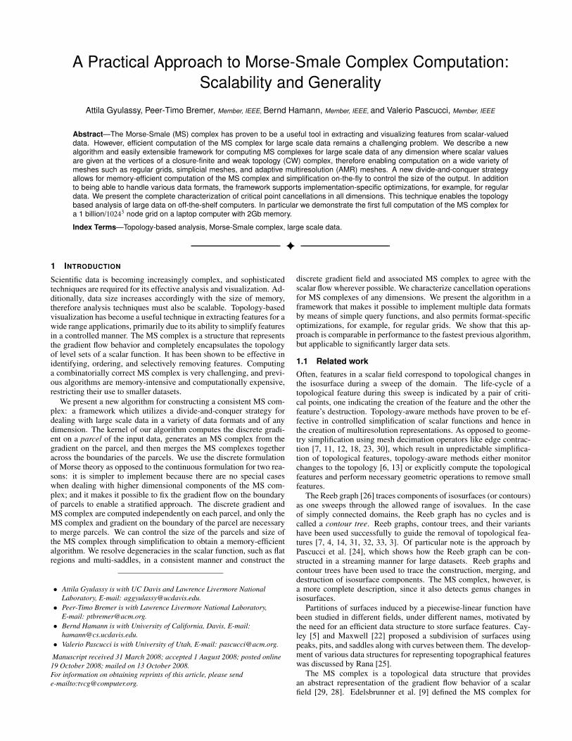
Fig. 1. A discrete Morse function (left) assigned to the simplices of asimple circle. The associated discrete gradient field (right) is a pairingof the vertices and edges. Note that the critical simplices of the discreteMorse function correspond exactly to the unpaired simplices of the dis-crete gradient field. In both cases, the vertex f−1(0) and the edge f−1(7)are the minimum and maximum respectively.

2.1 Morse Functions and the Morse-Smale ComplexA real-valued smooth map f : M → R defined over a compact d-manifold M is a Morse function if all its critical points are non-degenerate (i.e., the Hessian matrix is non-singular for all criticalpoints) and no two critical points have the same function value. Anintegral line of f is a maximal path in M whose tangent vectors agreewith the gradient of f at every point of the path. Each integral linehas a natural origin and destination at critical points of f where thegradient becomes zero. Ascending and descending manifolds are ob-tained as clusters of integral lines having common origin and desti-nation respectively. The Morse-Smale (MS) complex, denoted Γ, is apartition of M into regions clustering integral lines that share commonorigin and destination. In Morse-Smale functions, the integral linesonly connect critical points of different indices.

Each critical point of index n is the origin of a set of integral linesthat forms an ascending d−n-manifold. Symmetrically, it is the des-tination of a set of integral lines that forms a descending n-manifold.All ascending and descending manifolds of a Morse-Smale functionintersect transversally. Therefore, given two critical points a and b,where the index of a is one less than the index of b, the intersection ofthe ascending manifold of a and the descending manifold of b is eitherempty or a 1-manifold. The critical points and these 1-manifolds arecalled nodes and arcs. The one-skeleton formed by the nodes and arcsforms the combinatorial structure of the MS complex. The combina-torial structure contains much of the semantic information of f , andis useful for simplification and feature identification. The neighbor-hood of a node a of an MS complex Γ is the set of nodes Na that areconnected to a by an arc in Γ.

2.2 Discrete Morse TheoryThe discrete Morse theory introduced by Forman [10], is a paralleltheory to smooth Morse theory, and shows how to apply principlesfrom smooth theory to the discrete setting. We present some basicdefinitions from discrete Morse theory. A d-cell is a topological spacethat is homeomorphic to a d-ball Bd = {x ∈ Ed : |x| ≤ 1}. For cellsα and β , α < β means that α is a face of β and β is a co-face ofα , i.e., the vertices of α are a proper subset of the vertices of β . Ifdim(α) = dim(β )−1, we say α is a facet of β , and β is a co-facet ofα . A cell α has dimension d, and we denote this as α(d).

A finite CW-complex is a topological space X such that there existsa finite-nested sequence

/0⊂ X0 ⊂ X1 ⊂ ·· · ⊂ Xn = X

such that for each i = 0, 1, 2, ... , n, Xi is the result of attaching acell to X(i−1). A regular CW complex is a finite CW-complex, whereany two incident cells ρ and τ with dim(τ) = dim(ρ)− 2, there areexactly two cells σ1 and σ2 such that τ < σ1 < ρ and τ < σ2 < ρ .This requirement imposes restrictions on the attaching map, forcing

(a) (b)

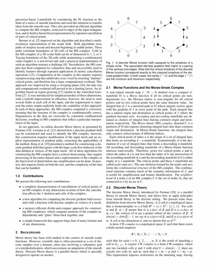
Fig. 2. The circled arc connects a saddle l to a maximum u (a). Can-cellation of (l,u) removes all arcs attached to l or u, and creates newarcs from the lower neighbors of u to the upper neighbors of l (b). In thetwo-dimensional case, this connects all the saddles neighboring u to themaximum neighboring l, in effect, merging l and u with the maximum).

the entire boundary of an attached cell to be glued to the topologicalspace, and restricting the boundary of a d-cell to be homeomorphic toa (d−1)-sphere.

Let K be a regular complex that is a mesh representation of M. Afunction f : K → R that assigns scalar values to every cell of K is adiscrete Morse function if for every α(d) ∈ K, its number of co-faces|{β (d+1) > α| f (β )≤ f (α)}| ≤ 1, and its number of faces |{γ(d−1) <

α| f (γ) ≥ f (α)}| ≤ 1. A cell α(d) is critical if its number of co-faces|{β (d+1) > α| f (β )≤ f (α)}|= 0 and its number of faces |{γ(d−1) <α| f (γ)≥ f (α)}|= 0. Figure 1 illustrates these configurations.

A vector in the discrete sense is a pair of cells {α(d) < β (d+1)},where we say that an arrow points from α(d) to β (d+1). Intuitively,this simulates a direction of flow. A discrete vector field V on K is acollection of pairs {α(d) < β (d+1)} of cells of K such that each cell isin at most one pair of V .

Given a discrete vector field V on K, a V -path is a sequence of cells

α(d)0 ,β

(d+1)0 ,α

(d)1 ,β

(d+1)1 ,α

(d)2 , . . . ,β

(d+1)r ,α

(d)r+1

such that for each i = 0,..., r, the pair {α(d) < β (d+1)} ∈ V , and{β (d+1)

i > α(d)i+1 6= α

(d)i }. A V -path is the discrete equivalent of a

streamline in a smooth vector field. A discrete vector field in whichall V -paths are monotonic and do not contain any loops is a discretegradient field. We will use V -paths to compute the MS complex of adiscrete gradient field.

2.3 Persistence-based SimplificationA function f is simplified by repeated cancellation of pairs of criticalpoints. The local change in the MS complex indicates the smootheningof the gradient vector field and hence of the function f . The orderingof critical point pairs is defined by persistence, which quantifies theimportance of the topological feature associated with a pair. The per-sistence of a critical point pair is the absolute difference in value off between the two points. We use the ordering given by persistenceto reduce the number of critical points and hence remove topologicalfeatures from f .

A cancellation operation is valid (i.e., it can be realized by a localperturbation of the gradient vector field) on a pair of critical points ifand only if there is exactly one arc connecting them in the complex.Therefore, the indices of the two critical points must differ by one.Also, any critical point pair that is connected by multiple arcs repre-sents a configuration known as a strangulation or a pouch, for whichthere is no direct perturbation of the gradient that removes the criticalpoint pair.

We characterize the cancellation operation for MS complexes ofany dimensions in terms of a change in the combinatorial structure ofthe complex. The geometric change in the manifolds of critical pointscan be derived from this combinatorial change.

Cancellation: Let Γ be an MS complex for a scalar function de-fined on a closed d-manifold M. Let l and u be the lower and uppernodes of an arc a in Γ, with index i and i + 1 respectively. Let Al be

the set of arcs that have l as one end point, Au the set of arcs that haveu as one end point, Nl the set of nodes in the neighborhood of l, andNu the set of nodes in the neighborhood of u.

The combinatorial cancellation of (l,u) changes the combinatorialstructure of the MS complex and is characterized as follows:

1. Create a new arc connecting every critical point of index i+1 inNl to every critical point of index i in Nu, and add them to Γ.

2. All arcs in Al , Au are removed from the complex, and l and u arealso removed from the complex.

This operation changes the 1-skeleton of the MS complex, how-ever, it also represents a change in the embedding. This change canbe derived from the combinatorial cancellation, and one simple wayto maintain a valid embedding is to characterize it as a merging ofthe manifolds of the nodes involved in the cancellation. We call thechange in the embedding the geometric realization of the cancellationand it is characterized as follows:

1. For every node of index i + 1 in Nl , merge its descending mani-fold with the descending manifold of u.

2. For every node of index i in Nu, merge its ascending manifoldwith the ascending manifold of l.

The cells of Γ after the cancellation are only different where thereare new intersections of the changed ascending and descending mani-folds. These intersections are represented by the new arcs in the com-binatorial structure of the MS complex. Although there are potentially|Nl | × |Nu| new arcs and cells created in the complex, the number ofnodes in the complex is reduced by two, and eventually all the newarcs are also removed in saddle-extremum cancellations. Figure 2illustrates this cancellation operation in the case of two-dimensionalcomplexes.

3 ALGORITHM

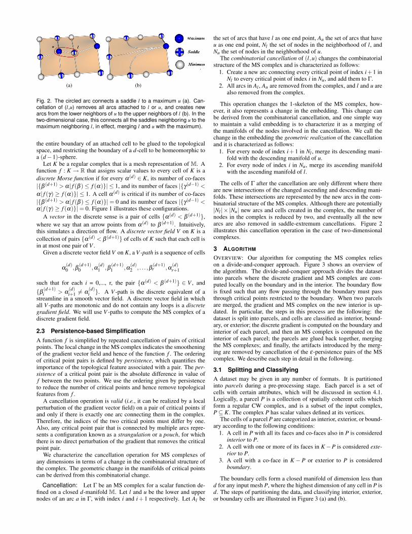
OVERVIEW: Our algorithm for computing the MS complex relieson a divide-and-conquer approach. Figure 3 shows an overview ofthe algorithm. The divide-and-conquer approach divides the datasetinto parcels where the discrete gradient and MS complex are com-puted locally on the boundary and in the interior. The boundary flowis fixed such that any flow passing through the boundary must passthrough critical points restricted to the boundary. When two parcelsare merged, the gradient and MS complex on the new interior is up-dated. In particular, the steps in this process are the following: thedataset is split into parcels, and cells are classified as interior, bound-ary, or exterior; the discrete gradient is computed on the boundary andinterior of each parcel, and then an MS complex is computed on theinterior of each parcel; the parcels are glued back together, mergingthe MS complexes; and finally, the artifacts introduced by the merg-ing are removed by cancellation of the ε-persistence pairs of the MScomplex. We describe each step in detail in the following.

3.1 Splitting and ClassifyingA dataset may be given in any number of formats. It is partitionedinto parcels during a pre-processing stage. Each parcel is a set ofcells with certain attributes, which will be discussed in section 4.1.Logically, a parcel P is a collection of spatially coherent cells whichform a regular CW complex, and is a subset of the input complex,P⊆ K. The complex P has scalar values defined at its vertices.

The cells of a parcel P are categorized as interior, exterior, or bound-ary according to the following conditions:

1. A cell in P with all its faces and co-faces also in P is consideredinterior to P.

2. A cell with one or more of its faces in K−P is considered exte-rior to P.

3. A cell with a co-face in K − P or exterior to P is consideredboundary.

The boundary cells form a closed manifold of dimension less thand for any input mesh P, where the highest dimension of any cell in P isd. The steps of partitioning the data, and classifying interior, exterior,or boundary cells are illustrated in Figure 3 (a) and (b).

(a) (b) (c)

(d) (e) (f)

(g) (h)

Fig. 3. An overview of the algorithm. The dataset (a) is broken up (b) into parcels, and cells are classified as interior (grey), exterior (green), orboundary (orange). The discrete gradient is found on the boundary and interior of each parcel (c) and the MS complex is computed (d). The parcelsare merged, reclassifying boundary and exterior cells (e), and the discrete gradient is computed on the newly introduced boundary and interiorcells (f). The complex is computed in these cells to complete the merging process (g). Simplification of ε-persistence pairs removes artifacts thathave resulted from merging (h).

3.2 Computing the Discrete Gradient

Given a regular CW-complex K with scalar values defined at the ver-tices and cells of dimension d and lower, we compute the discretegradient by assigning gradient arrows in a greedy manner in orderedsweeps over cells of K of increasing dimension, done by this algo-rithm:

1: for i ∈ [0, ..,d] do2: Iter = K→sortedCellIterator(i)3: while Iter→hasNext() do4: cellID = Iter→Item()5: if ! K→isMarked(cellID) then6: if K→hasPairableCoFacet(cellID) then7: pairID = K→lowestPairableCoFacet(cellID)8: K→pair(cellID,pairID )9: K→mark(cellID); K→mark(pairID)

10: else11: K→setCritical(cellID)12: K→mark(cellID)13: end if14: end if15: end while16: end for

This algorithm iterates through all cells in increasing order of di-mension and function value, assigning gradient pairs in a greedymanner. The sortedCellIterator(i) iterates through the i-cells ofK in order of increasing function value. The lowest cell of di-mension i that has not been paired or set as critical is cellID,and its co-facets are searched for a possible pair. The functionhasPairableCoFacet(cellID) returns true if there is a co-facet with ex-actly one facet that is not marked. If there are multiple such co-facetslowestPairableCoFacet(cellID) will return the lowest one. While anypairable co-facet could be paired with the cell, we select the one in thedirection of steepest descent to represent gradient flow of the function.When pair(cellID, pairID) forms a gradient arrow, the cell is set asthe head and the co-facet is marked as the tail.

The discrete vector field that is produced is a discrete gradient field,since each cell is paired exactly once, and no loops can be created inV -paths, since each V -path has a critical cell as a source that cannot befurther paired. The flow across cells in a discrete Morse function doesnot necessarily correspond to scalar flow. However, we assign functionvalues to all cells in a manner that allows gradient arrows to agree withthe scalar flow. The particular sorting order of the cells of a dimensiongiven by sorted cell iterator (line 2) and the lowest facet selected forpairing (line 7) determine the shape of the discrete gradient flow. If

the sorting is done from lowest to highest, and the facet selected is inthe direction of steepest descent, the discrete gradient flow generatedwill mostly agree with the scalar gradient.

Augmented Function The sorting of all the cells of a particulardimension requires function values to be assigned to every cell. Weuse the augmented function F , where each cell has a function valueslightly larger than the highest value of its faces:

F(α) = MAX{σ : σ < α}+ ε

In this manner, every cell is a critical cell in the discrete sense, and theformation of pairs performed by the algorithmic kernel corresponds toan ε-persistence cancellation of adjacent critical cells. We use sym-bolic perturbation to resolve the sorting order of two cells with thesame function value.

Gradient on a Parcel Although the gradient computation kerneloperates on any regular CW-complex, when computing the discretegradient of a parcel we impose some restrictions. The boundary cellsof a parcel represent the interface where flow can pass from one parcelto the next when the parcels are merged later on. To keep this inter-face as simple as possible, we first compute the discrete gradient onthe boundary of a parcel and then on the interior. This re-ordering en-sures that no boundary cell will be paired with an interior cell. Themotivation behind this reordering is to restrict the number of placeswhere flow can enter/exit the parcel from/to another parcel to the crit-ical points on the boundary. This is an important property that willmake merging parcels possible in subsequent steps of the algorithm.The computation of a gradient is a step in the algorithm shown in Fig-ure 3(c), where the gradient is first computed on each parcel, and thenthe gradient is computed in the interior.

3.3 The MS Complex on a Parcel

The MS complex of a discrete gradient vector field is uniquely de-termined by the gradient paths. To compute an MS complex fromthe discrete gradient vector field produced by the algorithm kernel, wefind the critical cells, and compute the ascending and descending man-ifolds by following the gradient paths. All the cells of a path whoseorigin is a critical cell α belong to the ascending manifold of α . Sym-metrically, all the cells of a path whose destination is a critical cell β

belong to the descending manifold of β . These paths are computedusing a depth-first search through the discrete gradient field. The cellsof the MS complex are attained as the intersection of ascending anddescending manifolds. The nodes and arcs forming the combinatorialstructure of the complex are the critical cells and the gradient pathsconnecting the critical cells.

Computing the ascending and descending manifolds requires acomplete traversal of the gradient paths. Our algorithm computes allcells of the MS complex. However, many cases arise where analysis ofthe data only requires the combinatorial structure (1-skeleton) of theMS complex. In this case, we can perform a more efficient compu-tation by only tracing ascending manifolds. Nevertheless, computingthe ascending manifolds of all minima requires a complete traversalof the entire gradient field. If we are only interested in the combi-natorial structure of the complex, this traversal is not necessary, andwe compute 1-saddle-minima connections by tracing gradient pathsdownwards from the 1-saddles. It is guaranteed that there are exactlytwo paths that terminate at a minimum for each 1-saddle, and the pathscannot split. This makes the computation of 1-saddle minimum con-nections efficient.

In general, ascending and descending manifolds can merge in a dis-crete gradient field. We maintain the MS complex by simulating aseparation between ascending manifolds and descending manifolds.The result of computing the MS complex on a parcel is shown in Fig-ure 3(d). Note that one major advantage of using discrete Morse theoryis that special rules for identifying manifolds of different dimensionsare not required, as was the case in [17].

3.4 Merging ParcelsMerging two parcels is a three-step process that involves gluing thetwo meshes together and updating and classification of cells, comput-ing the discrete gradient on the new boundary and interior, and finallymerging the two MS complexes. Two meshes are glued together byupdating the interior, boundary, or exterior classification on its cells.The interior cells remain interior, while the boundary cells can becomeinterior cells or remain boundary, and the exterior cells can become in-terior or boundary or remain exterior. The same rules apply that werepresented in section 3.1 for determining this classification. Figure 3 (e)shows the new classification of cells after this first step in the mergingprocess.

We repeat the algorithmic kernel for finding the discrete gradientfield on the merged parcels. First the gradient is computed for thecells that became boundary in the first step of the merging process,and then the gradient is computed for the cells that became interior inthe first step of the merging process. Figure 3 (f) shows the discretegradient computed on the new boundary and in the interior cells.

Finally, the MS complexes of each parcel are merged. Due to theway we first computed the discrete gradient on the boundary and thenin the interior in section 3.3, flow can only enter or leave a parcelthrough its boundary critical points. Therefore, we extend the MScomplex in each parcel by tracing gradient paths from all the newlyclassified interior and boundary critical cells. The only possible newconnections in the merged MS complex are between newly classifiedinterior critical cells. This fact makes it possible to remove the dis-crete gradient on the interior of each parcel from memory prior to themerging process, allowing for the memory-efficiency of the divide-and-conquer approach. Figure 3 (g) shows how the complexes aremerged by connecting them with critical cells in the new boundaryand in the interior.

Artifact Removal The merging of two parcels results in an MScomplex on the new parcel with “extra” nodes and arcs where the oldboundaries were. These extra nodes and arcs have low persistence, andare removed by canceling all ε-persistence pairs in the MS complex ofa parcel. Figure 3 (h) shows how the MS complex in the interior iscleaned up by canceling low-persistence arcs.

4 A FRAMEWORK FOR GENERALITY

The algorithm described in the previous section relies on queries thatare supported by a wide range of data formats. The internal repre-sentation of a parcel can vary based on the needs or optimizationspossible for any particular data format. For example, for regular data,the connectivity and classification of cells is attainable directly fromtheir indices and the extents of the parcel, therefore the queries canbe resolved in an efficient manner. A more general data format, suchas an AMR grid, or simplicial complex, may require a more elaboratestorage mechanism. The data format handles queries regarding char-acteristics of the cells in a parcel as well as the connectivity of the cellswithin that parcel.

4.1 Queries on the ParcelTo compute the discrete gradient, certain queries must be implementedfor the data structure. Given a unique identifier id for a cell, our im-plementation supports these functions:

• dimension(id): returns the dimension of the cell• isPaired(id): returns true if the cell has been paired• isPairable(id): returns true if the cell has one unpaired facet• greaterThan(id1, id2): returns true if id1 has higher function

value than id2

A parcel must also be able to provide iterators that access cells andtheir neighbors, which are implemented by these functions:

• d-cellIterator(): returns an iterator over all d-dimensional cellsin the parcel in sorted order

• boundary-d-cellIterator(): returns an iterator over all d-dimensional cells on the boundary of a parcel in sorted order

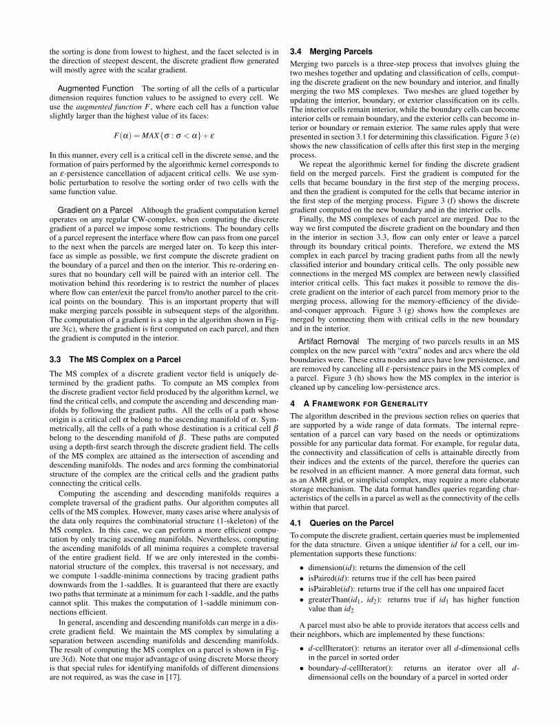
Fig. 4. A new slice is created to be merged with pbase. The orange cellsmark boundary, the green mark exterior, and the grey area indicates theprocessed interior of pbase.

• neighborIterator(id): returns an iterator over the facets and co-facets of a cell

Finally, a parcel must also be able to change the state of some of itscells, which is enabled by the following functions:

• markCritical(id): marks the particular cell as a critical cell• markAndPair(id1, id2): marks both as paired, and sets the pair of

each to the other

To compute the MS complex from the discrete gradient field, thefollowing queries must be supported:

• criticalPointIterator(): returns an iterator over the critical pointsin a parcel

• getPair(id): returns the identifier of the cell that id is paired with

Finally, the queries necessary for visualization of the complex re-quire that the geometric information of a cell can be recovered fromits identifier:

• getGeometry(id): returns an array of vertices that are the 0-dimensional faces of id

4.2 Flow of ControlThe basic steps of the algorithm discussed in section 3 are used tocompute and merge the MS complex on parcels, however, the order inwhich computation and merging take place are regulated by the datamanager. The data manager is a data-format-specific module that or-ganizes the flow of computation for maximal efficiency. In fact, eachdataset may have its own data manager to optimize for any structuralproperties of the data format or feature queries in the function.

The details of dividing the data into parcels, ordering the computa-tion of the gradient and MS complex on parcels, ordering the mergingof parcels, and any on-the-fly simplification of the MS complex areleft to the implementation. The interface with the algorithm is definedby the following functions:

1. computeGradAndComplex(Parcel p): computes the gradient andMS complex on boundary of a parcel; the results are stored in thestate of p. Additionally, the parcel is prepared for merging, byremoving the interior cells from memory.

2. merge(Parcel p1, Parcel p2): combines p1 and p2 into p1, in-ternally updating interior, boundary, and exterior classifications,computing the discrete gradient on the new boundary and in-terior cells, merging the MS complexes, and performing an ε-persistence simplification. After merging, p2 is empty.

3. simplify(Parcel p, Filters f ): performs simplification of the MScomplex on p according to filters defined in f .

A parcel may only be merged with another if the gradient and MScomplex have been computed on its boundary and in its interior, or if itcomposed entirely of exterior cells. It is the responsibility of the datamanager to create parcels and load the data.

Case Study: Slices on a Grid The implicit structure of datadefined on a regular grid (with inherent indices i, j, and k) can beexploited to achieve an efficient implementation. For example, thedimension, geometric location, and neighbors of a cell can be derivedfrom its index in the cases of simple Cartesian or uniformly spacedrectilinear grids. Also, rectangular parcels can be defined as lower andupper extents in each dimension. In this case, the extents determinewhether a cell is interior, exterior, or boundary. Merging the meshesof two aligned parcels can be accomplished by simply modifying theextents. All these properties make it possible to devise highly efficientimplementations of the queries on the parcel and its cells.

In the following, we consider the simple case of a dataset definedon a rectilinear grid with uniform spacing, aligned with the three co-ordinate axes. The simplest possible data manager creates a parcel forevery slice along one axis of the data. For example, in a 3D uniformrectilinear axis-aligned grid of size X ×Y ×Z, the data manager cre-ates an X ×Y parcel for every z value. Although there are many waysto order the creation and merging of parcels, the simplest way is toaccumulate them in a growing parcel along one axis. In this case thedata manager would operate as follows:

1: Parcel pbase = empty2: for z ∈ [0, ..,Z−1] do3: Parcel slice = createXYSlice(z)4: computeGradAndComplex(slice)5: merge(pbase, slice)6: simplify(pbase, filters)7: end for

Here the createXYSlice(z) reads the data from the input file corre-sponding the the XY slice at z and initializes state variables in the slice.The slice that is created is an array of size X×Y ×8, required for stor-ing the eight cells for every vertex of the data. The slices are mergedwith pbase, until pbase contains the complex of the entire mesh. Fig-ure 4 shows the addition of a slice onto pbase. The simplification stepcontrols the size of the complex as each slice is added on.

5 RESULTS

We provide results for data given on a uniform rectilinear grid, usingthe slicing data manager. The results were generated on an off-the-shelf 2.21GHz AMD Athlon with 2.0Gb memory, the same hardwareconfiguration used in [17]. We compare the performance of our algo-rithm to the previously fastest approach [17] in Table 1. Our run timesare similar, however, while the approach in [17] has a dataset size limitof 256× 256× 256, we also have produce results for one timestep ofa simulation of a Raleigh-Taylor instability, which has a resolution of1152× 1152× 1000, shown in Figure 5. In Laney et al. [20], a param-eter was used to select a 2-manifold level set, and the two-dimensionalMS complex used on the height map to identify bubbles in the turbu-lent mixing layer. A similar kind of analysis is possible using the fullcomplex we computed of the three-dimensional data without the needfor parameter selection, nevertheless, performing this kind of in-depthanalysis is beyond the scope of this paper. Our run times are largerfor the small data set sizes because we simplify ε-persistence arcs onthe fly, incorporating some of the post-processing into the construc-tion time. The results of [17] do not include this extra time neededfor simplification, and the complex extracted by that method must besimplified to remove noise and attain an MS complex comparable tothe result of our approach. Nevertheless, the optimizations made pos-sible by our general framework make the run times similar. The size ofthe memory footprint was controlled by the on-the-fly simplification,with the overhead for storing parcels being 42Mb, and the size of thecomplex kept under 1.3Gb.

6 ANALYSIS OF THE ALGORITHM

RUN TIME ANALYSIS The run time analysis of the complete algo-rithm is heavily dependent on the particular implementation of parcelsand the data manager. The run time analysis of the particular stepsof the algorithm can be performed using certain reasonable assump-tions, such as access to the faces and co-faces of a cell requiring

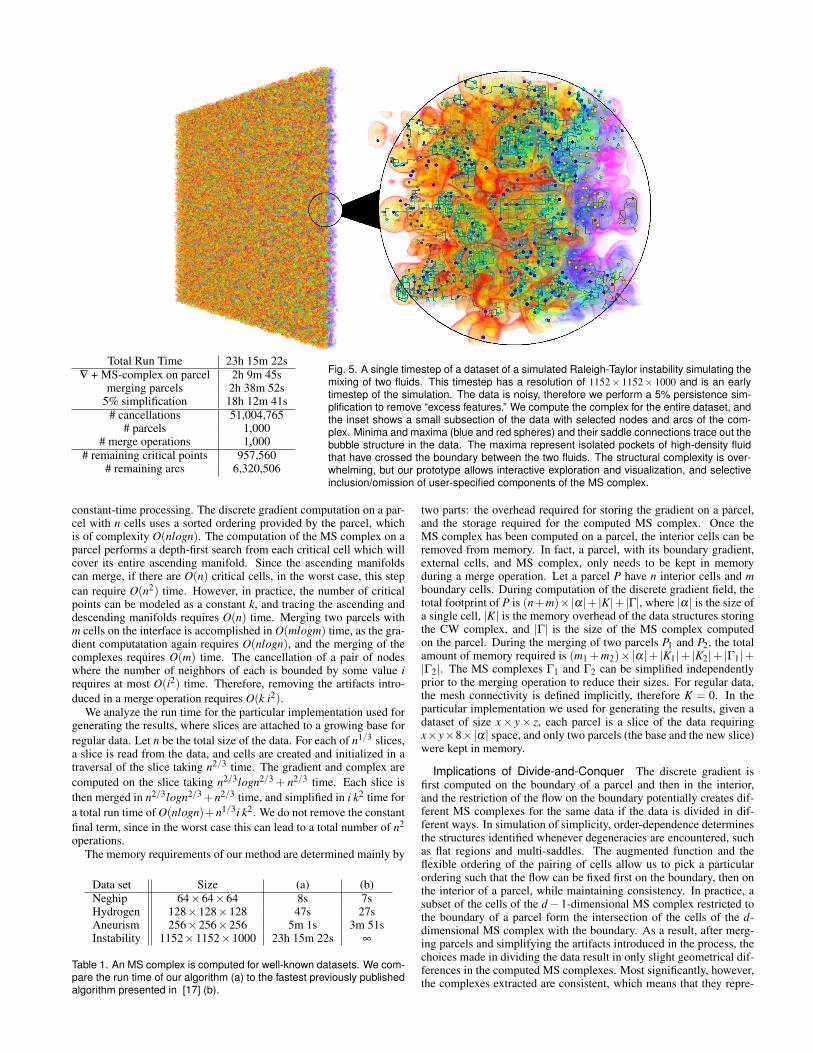
Total Run Time 23h 15m 22s∇ + MS-complex on parcel 2h 9m 45s

merging parcels 2h 38m 52s5% simplification 18h 12m 41s

# cancellations 51,004,765# parcels 1,000

# merge operations 1,000# remaining critical points 957,560

# remaining arcs 6,320,506

Fig. 5. A single timestep of a dataset of a simulated Raleigh-Taylor instability simulating themixing of two fluids. This timestep has a resolution of 1152× 1152× 1000 and is an earlytimestep of the simulation. The data is noisy, therefore we perform a 5% persistence sim-plification to remove “excess features.” We compute the complex for the entire dataset, andthe inset shows a small subsection of the data with selected nodes and arcs of the com-plex. Minima and maxima (blue and red spheres) and their saddle connections trace out thebubble structure in the data. The maxima represent isolated pockets of high-density fluidthat have crossed the boundary between the two fluids. The structural complexity is over-whelming, but our prototype allows interactive exploration and visualization, and selectiveinclusion/omission of user-specified components of the MS complex.

constant-time processing. The discrete gradient computation on a par-cel with n cells uses a sorted ordering provided by the parcel, whichis of complexity O(nlogn). The computation of the MS complex on aparcel performs a depth-first search from each critical cell which willcover its entire ascending manifold. Since the ascending manifoldscan merge, if there are O(n) critical cells, in the worst case, this stepcan require O(n2) time. However, in practice, the number of criticalpoints can be modeled as a constant k, and tracing the ascending anddescending manifolds requires O(n) time. Merging two parcels withm cells on the interface is accomplished in O(mlogm) time, as the gra-dient computatation again requires O(nlogn), and the merging of thecomplexes requires O(m) time. The cancellation of a pair of nodeswhere the number of neighbors of each is bounded by some value irequires at most O(i2) time. Therefore, removing the artifacts intro-duced in a merge operation requires O(k i2).

We analyze the run time for the particular implementation used forgenerating the results, where slices are attached to a growing base forregular data. Let n be the total size of the data. For each of n1/3 slices,a slice is read from the data, and cells are created and initialized in atraversal of the slice taking n2/3 time. The gradient and complex arecomputed on the slice taking n2/3logn2/3 + n2/3 time. Each slice isthen merged in n2/3logn2/3 +n2/3 time, and simplified in i k2 time fora total run time of O(nlogn)+n1/3i k2. We do not remove the constantfinal term, since in the worst case this can lead to a total number of n2

operations.The memory requirements of our method are determined mainly by

Data set Size (a) (b)Neghip 64×64×64 8s 7sHydrogen 128×128×128 47s 27sAneurism 256×256×256 5m 1s 3m 51sInstability 1152×1152×1000 23h 15m 22s ∞

Table 1. An MS complex is computed for well-known datasets. We com-pare the run time of our algorithm (a) to the fastest previously publishedalgorithm presented in [17] (b).

two parts: the overhead required for storing the gradient on a parcel,and the storage required for the computed MS complex. Once theMS complex has been computed on a parcel, the interior cells can beremoved from memory. In fact, a parcel, with its boundary gradient,external cells, and MS complex, only needs to be kept in memoryduring a merge operation. Let a parcel P have n interior cells and mboundary cells. During computation of the discrete gradient field, thetotal footprint of P is (n+m)×|α|+ |K|+ |Γ|, where |α| is the size ofa single cell, |K| is the memory overhead of the data structures storingthe CW complex, and |Γ| is the size of the MS complex computedon the parcel. During the merging of two parcels P1 and P2, the totalamount of memory required is (m1 +m2)×|α|+ |K1|+ |K2|+ |Γ1|+|Γ2|. The MS complexes Γ1 and Γ2 can be simplified independentlyprior to the merging operation to reduce their sizes. For regular data,the mesh connectivity is defined implicitly, therefore K = 0. In theparticular implementation we used for generating the results, given adataset of size x× y× z, each parcel is a slice of the data requiringx×y×8×|α| space, and only two parcels (the base and the new slice)were kept in memory.

Implications of Divide-and-Conquer The discrete gradient isfirst computed on the boundary of a parcel and then in the interior,and the restriction of the flow on the boundary potentially creates dif-ferent MS complexes for the same data if the data is divided in dif-ferent ways. In simulation of simplicity, order-dependence determinesthe structures identified whenever degeneracies are encountered, suchas flat regions and multi-saddles. The augmented function and theflexible ordering of the pairing of cells allow us to pick a particularordering such that the flow can be fixed first on the boundary, then onthe interior of a parcel, while maintaining consistency. In practice, asubset of the cells of the d−1-dimensional MS complex restricted tothe boundary of a parcel form the intersection of the cells of the d-dimensional MS complex with the boundary. As a result, after merg-ing parcels and simplifying the artifacts introduced in the process, thechoices made in dividing the data result in only slight geometrical dif-ferences in the computed MS complexes. Most significantly, however,the complexes extracted are consistent, which means that they repre-

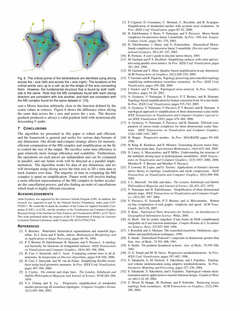
Fig. 6. The critical points of the tetrahedrane are identified using slicingacross the z axis (left) and across the x axis (right). The locations of thecritical points vary up to a cell, as do the shape of the arcs connectingthem. However, the fundamental structure that is found by both meth-ods is the same. Note that the MS complexes found with each slicingdirection are consistent with one another, and both are consistent withthe MS complex found for the same dataset in [15].

sent a Morse function arbitrarily close to the function defined by thescalar values at vertices. Figure 6 shows the difference when slicingthe same data across the z axis and across the x axis. The discretegradient produced is always a valid gradient field with monotonicallydescending V -paths.

7 CONCLUSIONS

The algorithm we presented in this paper is robust and efficient,and the framework is general and works for various data formats ofany dimension. Our divide-and-conquer strategy allows for memory-efficient computation of the MS complex and simplification on the flyto control the size of the output. We sacrifice some time efficiency togain relatively more storage efficiency and scalability. Furthermore,the operations on each parcel are independent and can be computedin parallel, and our future work will be directed at a parallel imple-mentation. The algorithm works for data of any dimension, and wewill investigate using slicing across the time axis in 3D + time data totrack features over time. The majority of time in computing the MScomplex is spent on simplification. Future work will involve findinga more efficient representation of the MS complex to further acceler-ate the cancellation process, and also finding an order of cancellationswhich leads to highly efficient execution.

ACKNOWLEDGEMENTS

Attila Gyulassy was supported by the Lawrence Scholar Program (LSP). In addition, thisresearch was supported in part by the National Science Foundation, under grant CCF-0702817. We would like to thank the members of the Center for Applied Scientific Com-puting (CASC), at LLNL, and the members of the Visualization and Computer GraphicsResearch Group of the Institute for Data Analysis and Visualization (IDAV), at UC Davis.This work performed under the auspices of the U.S. Department of Energy by LawrenceLivermore National Laboratory under Contract DE-AC52-07NA27344.

REFERENCES

[1] S. Beucher. Watershed, heirarchical segmentation and waterfall algo-rithm. In J. Serra and P. Soille, editors, Mathematical Morphology andits Applications to Image Processing, pages 69–76, 1994.

[2] P.-T. Bremer, H. Edelsbrunner, B. Hamann, and V. Pascucci. A topolog-ical hierarchy for functions on triangulated surfaces. IEEE Transactionson Visualization and Computer Graphics, 10(4):385–396, 2004.

[3] H. Carr, J. Snoeyink, and U. Axen. Computing contour trees in all di-mensions. In Symposium on Discrete Algorithms, pages 918–926, 2000.

[4] H. Carr, J. Snoeyink, and M. van de Panne. Simplifying flexible isosur-faces using local geometric measures. In Proc. IEEE Conf. Visualization,pages 497–504, 2004.

[5] A. Cayley. On contour and slope lines. The London, Edinburgh andDublin Philosophical Magazine and Journal of Science, XVII:264–268,1859.

[6] Y.-J. Chiang and X. Lu. Progressive simplification of tetrahedralmeshes preserving all isosurface topologies. Computer Graphics Forum,22(3):493–504, 2003.

[7] P. Cignoni, D. Constanza, C. Montani, C. Rocchini, and R. Scopigno.Simplification of tetrahedral meshes with accurate error evaluation. InProc. IEEE Conf. Visualization, pages 85–92, 2000.

[8] H. Edelsbrunner, J. Harer, V. Natarajan, and V. Pascucci. Morse-Smalecomplexes for piecewise linear 3-manifolds. In Proc. 19th Ann. Sympos.Comput. Geom., pages 361–370, 2003.

[9] H. Edelsbrunner, J. Harer, and A. Zomorodian. Hierarchical Morse-Smale complexes for piecewise linear 2-manifolds. Discrete and Compu-tational Geometry, 30(1):87–107, 2003.

[10] R. Forman. A user’s guide to discrete morse theory, 2001.[11] M. Garland and P. S. Heckbert. Simplifying surfaces with color and tex-

ture using quadric error metrics. In Proc. IEEE Conf. Visualization, pages263–269, 1998.

[12] M. Garland and Y. Zhou. Quadric-based simplification in any dimension.ACM Transactions on Graphics, 24(2):209–239, 2005.

[13] T. Gerstner and R. Pajarola. Topology preserving and controlled topologysimplifying multiresolution isosurface extraction. In Proc. IEEE Conf.Visualization, pages 259–266, 2000.

[14] I. Guskov and Z. Wood. Topological noise removal. In Proc. GraphicsInterface, pages 19–26, 2001.

[15] A. Gyulassy, V. Natarajan, V. Pascucci, P.-T. Bremer, and B. Hamann.Topology-based simplification for feature extraction from 3d scalar fields.In Proc. IEEE Conf. Visualization, pages 535–542, 2005.

[16] A. Gyulassy, V. Natarajan, V. Pascucci, P. T. Bremer, and B. Hamann. Atopological approach to simplification of three-dimensional scalar fields.IEEE Transactions on Visualization and Computer Graphics (special is-sue IEEE Visualization 2005), pages 474–484, 2006.

[17] A. Gyulassy, V. Natarajan, V. Pascucci, and B. Hamann. Efficient com-putation of morse-smale complexes for three-dimensional scalar func-tions. IEEE Transactions on Visualization and Computer Graphics,13(6):1440–1447, 2007.

[18] H. Hoppe. Progressive meshes. In Proc. SIGGRAPH, pages 99–108,1996.

[19] H. King, K. Knudson, and N. Mramor. Generating discrete morse func-tions from point data. Experimental Mathematics, 14(4):435–444, 2005.

[20] D. Laney, A. Mascarenhas, and P. Miller. Understanding the structure ofthe turbulent mixing layer in hydrodynamic instabilities. IEEE Transac-tions on Visualization and Computer Graphics, 12(5):1053–1060, 2006.Member-P. -T. Bremer and Member-V. Pascucci.

[21] T. Lewiner, H. Lopes, and G. Tavares. Applications of forman’s discretemorse theory to topology visualization and mesh compression. IEEETransactions on Visualization and Computer Graphics, 10(5):499–508,2004.

[22] J. C. Maxwell. On hills and dales. The London, Edinburgh and DublinPhilosophical Magazine and Journal of Science, XL:421–427, 1870.

[23] V. Natarajan and H. Edelsbrunner. Simplification of three-dimensionaldensity maps. IEEE Transactions on Visualization and Computer Graph-ics, 10(5):587–597, 2004.

[24] V. Pascucci, G. Scorzelli, P.-T. Bremer, and A. Mascarenhas. Robuston-line computation of reeb graphs: simplicity and speed. ACM Trans.Graph., 26(3):58, 2007.

[25] S. Rana. Topological Data Structures for Surfaces: An Introduction toGeographical Information Science. Wiley, 2004.

[26] G. Reeb. Sur les points singuliers d’une forme de Pfaff completementintegrable ou d’une fonction numerique. Comptes Rendus de L’Academieses Seances, Paris, 222:847–849, 1946.

[27] J. Roerdink and A. Meijster. The watershed transform: Definitions, algo-rithms and parallelization techniques, 1999.

[28] S. Smale. Generalized Poincare’s conjecture in dimensions greater thanfour. Ann. of Math., 74:391–406, 1961.

[29] S. Smale. On gradient dynamical systems. Ann. of Math., 74:199–206,1961.

[30] O. G. Staadt and M. H. Gross. Progressive tetrahedralizations. In Proc.IEEE Conf. Visualization, pages 397–402, 1998.

[31] S. Takahashi, G. M. Nielson, Y. Takeshima, and I. Fujishiro. Topolog-ical volume skeletonization using adaptive tetrahedralization. In Proc.Geometric Modeling and Processing, pages 227–236, 2004.

[32] S. Takahashi, Y. Takeshima, and I. Fujishiro. Topological volume skele-tonization and its application to transfer function design. Graphical Mod-els, 66(1):24–49, 2004.

[33] Z. Wood, H. Hoppe, M. Desbrun, and P. Schroder. Removing excesstopology from isosurfaces. ACM Transactions on Graphics, 23(2):190–208, 2004.