a practical beginner s guide to cyclic voltammetry · a practical beginner’s guide to cyclic...

A Practical Beginner’s Guide to Cyclic VoltammetryNoemie Elgrishi, Kelley J. Rountree, Brian D. McCarthy, Eric S. Rountree, Thomas T. Eisenhart,and Jillian L. Dempsey*

Department of Chemistry, University of North Carolina, Chapel Hill, North Carolina 27599-3290, United States

*S Supporting Information

ABSTRACT: Despite the growing popularity of cyclic voltammetry, many students do notreceive formalized training in this technique as part of their coursework. Confronted withself-instruction, students can be left wondering where to start. Here, a short introduction tocyclic voltammetry is provided to help the reader with data acquisition and interpretation.Tips and common pitfalls are provided, and the reader is encouraged to apply what is learnedin short, simple training modules provided in the Supporting Information. Armed with thebasics, the motivated aspiring electrochemist will find existing resources more accessible andwill progress much faster in the understanding of cyclic voltammetry.

KEYWORDS: Upper-Division Undergraduate, Graduate Education/Research, Inorganic Chemistry, Analytical Chemistry,Distance Learning/Self Instruction, Inquiry-Based/Discovery Learning, Textbooks/Reference Books, Electrochemistry

■ INTRODUCTION

Motivation

Electron transfer processes are at the center of the reactivity ofinorganic complexes. Molecular electrochemistry has become acentral tool of research efforts aimed at developing renewableenergy technologies. As the field evolves rapidly, the need fora new generation of trained electrochemists is mounting.While several textbooks and online resources are available,1−5

as well as an increasing number of laboratories geared towardundergraduate students,6,7 no concise and approachable guide tocyclic voltammetry for inorganic chemists is available. Here, weupdate, build on, and streamline seminal papers8−11 to provide asingle introductory text that reflects the current best practices forlearning and utilizing cyclic voltammetry. Practical experimentsand examples centered on nonaqueous solvents are provided tohelp kick-start cyclic voltammetry experiments for inorganicchemists interested in utilizing electrochemical methods for theirresearch. The practical experiments in this text are the basis forthe instruction of new researchers in our laboratory.

Electrochemistry

Electrochemistry is a powerful tool to probe reactions involvingelectron transfers. Electrochemistry relates the flow of electrons tochemical changes. In inorganic chemistry, the resulting chemicalchange is often the oxidation or reduction of a metal complex.To understand the difference between a chemical reduction and anelectrochemical reduction, consider the example of the reductionof ferrocenium [Fe(Cp)2]

+ (Cp = cyclopentadienyl), abbreviatedas Fc+, to ferrocene [Fe(Cp)2], abbreviated as Fc:

• Through a chemical reducing agent: Fc+ + [Co(Cp*)2]⇌Fc + [Co(Cp*)2]

+

• At an electrode: Fc+ + e− ⇌ Fc

Why does [Co(Cp*)2] (Cp* = pentamethylcyclopentadienyl)reduce Fc+? In the simplest explanation, an electron transfersfrom [Co(Cp*)2] to Fc

+ because the lowest unoccupied molec-ular orbital (LUMO) of Fc+ is at a lower energy than the elec-tron in the highest occupied molecular orbital (HOMO) of[Co(Cp*)2]. The transfer of an electron between the twomoleculesin solution is thermodynamically favorable (Figure 1A), and thedifference in energy levels is the driving force for the reaction.In an electrochemical reduction, Fc+ is reduced via hetero-

geneous electron transfer from an electrode; but what is thedriving force for this process? An electrode is an electrical con-ductor, typically platinum, gold, mercury, or glassy carbon. Throughuse of an external power source (such as a potentiostat), voltagecan be applied to the electrode to modulate the energy of theelectrons in the electrode. When the electrons in the electrodeare at a higher energy than the LUMO of Fc+, an electron fromthe electrode is transferred to Fc+ (Figure 1B). The driving forcefor this electrochemical reaction is again the energy differencebetween that of the electrode and the LUMO of Fc+.Changing the driving force of a chemical reduction requires

changing the identity of the molecule used as the reductant.12

At its core, the power of electrochemistry resides in the simplicitywith which the driving force of a reaction can be controlled andthe ease with which thermodynamic and kinetic parameters canbe measured.

Received: May 26, 2017Revised: September 13, 2017Published: November 3, 2017

Article

pubs.acs.org/jchemeduc

© 2017 American Chemical Society andDivision of Chemical Education, Inc. 197 DOI: 10.1021/acs.jchemed.7b00361

J. Chem. Educ. 2018, 95, 197−206

This is an open access article published under an ACS AuthorChoice License, which permitscopying and redistribution of the article or any adaptations for non-commercial purposes.

Dow

nloa

ded

via

IND

IAN

IN

ST O

F T

EC

HN

OL

OG

Y K

AN

PUR

on

July

9, 2

018

at 0

9:59

:14

(UT

C).

Se

e ht

tps:

//pub

s.ac

s.or

g/sh

arin

ggui

delin

es f

or o

ptio

ns o

n ho

w to

legi

timat

ely

shar

e pu

blis

hed

artic

les.

http://pubs.acs.org/doi/suppl/10.1021/acs.jchemed.7b00361/suppl_file/ed7b00361_si_001.pdf

pubs.acs.org/jchemeduc

http://dx.doi.org/10.1021/acs.jchemed.7b00361

http://pubs.acs.org/page/policy/editorchoice/index.html

http://pubs.acs.org/page/policy/authorchoice_termsofuse.html

Cyclic Voltammetry

Cyclic voltammetry (CV) is a powerful and popular electro-chemical technique commonly employed to investigate the reduc-tion and oxidation processes of molecular species. CV is alsoinvaluable to study electron transfer-initiated chemical reactions,which includes catalysis. As inorganic chemists embrace electro-chemistry, papers in the literature often contain figures likeFigure 2.

The aim of this paper is to provide the readers with thetools necessary to understand the key features of Figure 2.The following section will provide clues to understand the data,the reason for including the experimental parameters, theirmeaning and influence, and a broader discussion about howto set up the experiment and what parameters to considerwhen recording your own data. Finally, a brief description offrequently encountered responses in cyclic voltammetry willbe given. The text will be punctuated with boxes containingfurther information (green) or potential pitfalls (red). Addi-tional callouts refer to short training modules provided in theSupporting Information (SI).

■ UNDERSTANDING THE SIMPLE VOLTAMMOGRAM

Cyclic Voltammetry Profile

The traces in Figure 2 are called voltammograms or cyclicvoltammograms. The x-axis represents a parameter that is

imposed on the system, here the applied potential (E), while they-axis is the response, here the resulting current (i) passed.The current axis is sometimes not labeled (instead a scale bar isinset to the graph). Two conventions are commonly used toreport CV data, but seldom is a statement provided that describesthe sign convention used for acquiring and plotting the data.However, the potential axis gives a clue to the convention used, asexplained in Box 1. Each trace contains an arrow indicating the

direction in which the potential was scanned to record the data.The arrow indicates the beginning and sweep direction of thefirst segment (or “forward scan”), and the caption indicates theconditions of the experiment. A crucial parameter can be found inthe caption of Figure 2: “υ = 100 mV/s”. This value is called thescan rate (υ). It indicates that during the experiment the potentialwas varied linearly at the speed (scan rate) of 100mV per second.Panel I of Figure 3 shows the relationship between time and

applied potential, with the potential axis as the x-axis to see therelation with the corresponding voltammogram in panel H.In this example, in the forward scan, the potential is sweptnegatively from the starting potential E1 to the switchingpotential E2. This is referred to as the cathodic trace. The scandirection is then reversed, and the potential is swept positivelyback to E1, referred to as the anodic trace.13−15

Understanding the “Duck” Shape: Introduction to theNernst Equation

Why are there peaks in a cyclic voltammogram? Consider theequilibrium between ferrocenium (Fc+) and ferrocene (Fc).This equilibrium is described by the Nernst equation (eq 1).The Nernst equation relates the potential of an electrochemical

Figure 1. (A) Homogeneous and (B) heterogeneous reduction of Fc+ to Fc. The energy of the electrons in the electrode is controlled by thepotentiostat; their energy can be increased until electron transfer becomes favorable.4

Figure 2. Voltammograms of a bare electrode under N2 (blue trace); abare electrode under air (red trace); [CoCp(dppe)(CH3CN)](PF6)2(dppe = diphenylphosphinoethane) under N2 (green trace); [CoCp-(dppe)(CH3CN)](PF6)2 under air (orange trace). Voltammogramsrecorded in 0.25M [NBu4][PF6] CH3CN solution at υ = 100mV/s witha 3 mm glassy carbon working electrode, a 3 mm glassy carbon counterelectrode, and a silver wire pseudoreference electrode.

Journal of Chemical Education Article

DOI: 10.1021/acs.jchemed.7b00361J. Chem. Educ. 2018, 95, 197−206

198



cell (E) to the standard potential of a species (E0) and the relativeactivities16 of the oxidized (Ox) and reduced (Red) analyte in thesystem at equilibrium. In the equation, F is Faraday’s constant,R is the universal gas constant, n is the number of electrons, andTis the temperature

= + = +E ERTnF

ERTnF

ln(Ox)

(Red)2.3026 log

(Ox)(Red)

0 010

(1)

In application of the Nernst Equation to the one-electronreduction of Fc+ to Fc, the activities are replaced with theirconcentrations, which are more experimentally accessible, thestandard potential E0 is replaced with the formal potential E0′,and n is set equal to 1:

= ′ + = ′ ++ +

E ERTF

ERTF

ln[Fc ][Fc]

2.3026 log[Fc ][Fc]

0 010

(2)

The formal potential is specific to the experimental conditionsemployed and is often estimated with the experimentally deter-mined E1/2 value (Figure 3, average potential between pointsF andC in panelH). TheNernst equation provides a powerful wayto predict how a systemwill respond to a change of concentrationof species in solution or a change in the electrode potential.To illustrate, if a potential of E = E°′ ≈ E1/2 is applied to ourexample Fc+ solution, the Nernst equation predicts that Fc+ willbe reduced to Fc until [Fc+] = [Fc], and equilibrium is achieved.Alternatively, when the potential is scanned during the CV experi-ment, the concentration of the species in solution near the elec-trode changes over time in accordance with the Nernst equation.When a solution of Fc+ is scanned to negative potentials, Fc+

is reduced to Fc locally at the electrode, resulting in themeasurement of a current and depletion of Fc+ at the electrodesurface. The resulting cyclic voltammogram is presented inFigure 3 as well as the concentration−distance profiles for Fc+(blue) and Fc (green) at different points in the voltammogram.Crucially, the concentrations of Fc+ vs Fc relative to the distance

from the surface of the electrode are dependent on the potentialapplied and how species move between the surface of theelectrode and the bulk solution (see below). These factors allcontribute to the “duck”-shaped voltammograms.As the potential is scanned negatively (cathodically) from

point A to pointD (Figure 3), [Fc+] is steadily depleted near theelectrode as it is reduced to Fc. At point C, where the peakcathodic current (ip,c) is observed, the current is dictated by thedelivery of additional Fc+ via diffusion from the bulk solution.The volume of solution at the surface of the electrode con-taining the reduced Fc, called the diffusion layer, continues to growthroughout the scan. This slows downmass transport of Fc+ to theelectrode. Thus, upon scanning to more negative potentials, therate of diffusion of Fc+ from the bulk solution to the electrodesurface becomes slower, resulting in a decrease in the current asthe scan continues (C→ D). When the switching potential (D)is reached, the scan direction is reversed, and the potentialis scanned in the positive (anodic) direction. While theconcentration of Fc+ at the electrode surface was depleted, theconcentration of Fc at the electrode surface increased, satisfyingthe Nernst equation. The Fc present at the electrode surface isoxidized back to Fc+ as the applied potential becomes morepositive. At points B and E, the concentrations of Fc+ and Fc atthe electrode surface are equal, following the Nernst equation,E = E1/2. This corresponds to the halfway potential between thetwo observed peaks (C and F) and provides a straightforwardway to estimate the E0′ for a reversible electron transfer, as notedabove. The two peaks are separated due to the diffusion of theanalyte to and from the electrode.If the reduction process is chemically and electrochemically

reversible, the difference between the anodic and cathodic peakpotentials, called peak-to-peak separation (ΔEp), is 57 mV at25 °C (2.22 RT/F), and the width at half max on the forward scanof the peak is 59 mV.3 Chemical reversibility is used to denotewhether the analyte is stable upon reduction and can sub-sequently be reoxidized. Analytes that react in homogeneouschemical processes upon reduction (such as ligand loss or

Figure 3. (A−G): Concentration profiles (mM) for Fc+ (blue) and Fc (green) as a function of the distance from the electrode (d, from the electrodesurface to the bulk solution, e.g. 0.5 mm) at various points during the voltammogram. Adapted from Reference 4. Copyright © 2011, Imperial CollegePress. (H): Voltammogram of the reversible reduction of a 1 mM Fc+ solution to Fc, at a scan rate of 100 mV s−1. (I): Applied potential as a function oftime for a generic cyclic voltammetry experiment, with the initial, switching, and end potentials represented (A, D, and G, respectively).



199


degradation) are not chemically reversible (see discussion belowon EC Coupled Reactions). Electrochemical reversibility refersto the electron transfer kinetics between the electrode andthe analyte. When there is a low barrier to electron transfer(electrochemical reversibility), the Nernstian equilibrium isestablished immediately upon any change in applied potential.By contrast, when there is a high barrier to electron transfer(electrochemical irreversibility), electron transfer reactions aresluggish and more negative (positive) potentials are requiredto observe reduction (oxidation) reactions, giving rise to largerΔEp. Often electrochemically reversible processeswhere theelectron transfers are fast and the processes follow the Nernstequationare referred to as “Nernstian.”Importance of the Scan Rate

The scan rate of the experiment controls how fast the appliedpotential is scanned. Faster scan rates lead to a decrease in thesize of the diffusion layer; as a consequence, higher currentsare observed.2,3 For electrochemically reversible electrontransfer processes involving freely diffusing redox species, theRandles−Sevcik equation (eq 3) describes how the peak currentip (A) increases linearly with the square root of the scan rateυ (V s−1), where n is the number of electrons transferred in theredox event, A (cm2) is the electrode surface area (usually treatedas the geometric surface area), Do (cm2 s−1) is the diffusioncoefficient of the oxidized analyte, and C0 (mol cm−3) is the bulkconcentration of the analyte.

υ= ⎜ ⎟⎛

⎝⎞⎠i nFAC

nF DRT

0.446p0 o

1/2

(3)

The Randles−Sevcik equation can give indications as towhether an analyte is freely diffusing in solution, as explained inBox 2. As analytes can sometimes adsorb to the electrode surface,it is essential to assess whether an analyte remains homogeneousin solution prior to analyzing its reactivity. In addition toverifying that the analyte is freely diffusing, the Randles−Sevcikequation may be used to calculate diffusion coefficients(Experimental Module 4: Cyclic Voltammetry of Ferrocene:Measuring a Diffusion Coefficient).2

■ COLLECTING DATA

Introduction to the Electrochemical Cell

In the experimental section of papers describing electrochemicalmeasurements, a brief description is generally given for theexperimental setup used to collect the data. The vessel used for acyclic voltammetry experiment is called an electrochemical cell.A schematic representation of an electrochemical cell is presentedin Figure 4. The subsequent sections will describe the role of eachcomponent and how to assemble an electrochemical cell to collectdata during CV experiments.Preparation of Electrolyte Solution

As electron transfer occurs during a CV experiment, electricalneutrality is maintained via migration of ions in solution.As electrons transfer from the electrode to the analyte, ions movein solution to compensate the charge and close the electricalcircuit. A salt, called a supporting electrolyte, is dissolved in thesolvent to help decrease the solution resistance. The mixture ofthe solvent and supporting electrolyte is commonly termed the“electrolyte solution.”Solvent. A good solvent has these characteristics:

• It is liquid at experimental temperatures.

• It dissolves the analyte and high concentrations of thesupporting electrolyte completely.

• It is stable toward oxidation and reduction in the potentialrange of the experiment.

• It does not lead to deleterious reactions with the analyte orsupporting electrolyte.

• It can be purified.

The potential windows of stability (“solvent window”) ofsome common solvents used for inorganic electrochemistry areshown in Box 3. Experimenters are advised to rigorously ensure

Figure 4. Schematic representation of an electrochemical cell for CVexperiments.



200



solvents are free of impurities and, if necessary, rigorouslyanhydrous.Supporting Electrolyte. A good supporting electrolyte has

these characteristics:

• It is highly soluble in the solvent chosen.• It is chemically and electrochemically inert in the

conditions of the experiment.• It can be purified.

Large supporting electrolyte concentrations are necessary toincrease solution conductivity. As electron transfers occur at theelectrodes, the supporting electrolyte will migrate to balancethe charge and complete the electrical circuit. The conductivityof the solution is dependent on the concentrations of the dis-solved salt. Without the electrolyte available to achievecharge balance, the solution will be resistive to charge transfer(see How To Minimize Ohmic Drop below). High absoluteelectrolyte concentrations are thus necessary.Large supporting electrolyte concentrations are also necessary

to limit analyte migration. Movement of the analyte to theelectrode surface is controlled by three modes of mass transport:convection, migration, and diffusion. A species that moves byconvection is under the action of mechanical forces (e.g., stirringor vibrations). In migration, ionic solute moves by action of anelectric field (e.g., positive ions are attracted to negative elec-trodes). Diffusion arises from a concentration difference betweentwo points within the electrochemical cell; this concentrationgradient results in analyte movement from areas of high to areasof low concentration. All theoretical treatments and modelingexclude migration and convection of the analyte. To ensure thatthese mechanisms of mass transport are minimized, convection isreduced by the absence of stirring or vibrations, and migration isminimized through the use of electrolyte in high concentra-tion.2 High electrolyte concentration relative to the analyte

concentration ensures that it is statistically more probable thatthe electrolyte will migrate to the electrode surface for chargebalance.Ammonium salts have become the electrolyte of choice for

inorganic electrochemistry experiments performed in organicsolvents as they fulfill the three conditions of electrolyte choice.For dichloromethane or acetonitrile solutions, tetrabutylammo-nium (+NBu4) salts are commonly used. For less polar solventslike benzene, tetrahexylammonium salts are more soluble.While ammonium salts have become the standard cation, thechoice of counteranion is less standardized as anions tend to bemore reactive with transition metal analytes. The most commonlyused anions are [B(C6F5)4]¯, [B(C6H5)4]¯, [PF6]¯, [BF4]¯, and[ClO4]¯. The more coordinating the anion, the more likely it is tohave unwanted interactions with the cation, the solvent, or theanalyte. We have found [NBu4][PF6] salts to be ideal supportingelectrolytes in acetonitrile for their stability, noncoordinatingnature, ease of purification, and solubility. Purity of the electro-lyte is paramount because of the high concentrations required(we routinely use 0.25M [NBu4][PF6] inCH3CN),meaning eventhe slightest impurity can reach a concentration sufficient to inter-fere with the measurement. For information on the purificationof common electrolyte salts, we direct the reader to page 70 ofreference 1.

Choosing Electrodes and Preparing Them for Use

The caption of Figure 2 indicates that a three-electrode setup wasused, including a glassy carbon working electrode, glass carboncounter electrode, and Ag+/Ag pseudoreference electrode.This setup (Figure 4) is typical for common electrochemicalexperiments, including cyclic voltammetry, and the threeelectrodes represent a working electrode, counter elec-trode, and reference electrode, respectively. While the currentflows between the working and counter electrodes, the referenceelectrode is used to accurately measure the applied potentialrelative to a stable reference reaction.

Working Electrode (WE).The working electrode carries outthe electrochemical event of interest. A potentiostat is used tocontrol the applied potential of the working electrode as a func-tion of the reference electrode potential. The most importantaspect of the working electrode is that it is composed of redox-inert material in the potential range of interest. The type ofworking electrode can be varied from experiment to experimentto provide different potential windows or to reduce/promotesurface adsorption of the species of interest (see Box 3 forexamples).Because the electrochemical event of interest occurs at the

working electrode surface, it is imperative that the electrodesurface be extremely clean and its surface area well-defined.The procedure for polishing electrodes varies based on the typeof electrode and may vary from lab to lab. When using electrodessuch as glassy carbon or platinum, clean electrodes surfacescan be prepared via mechanical polishing (Box 4). To removeparticles, the electrode is then sonicated in ultrapure water.17 It isoften also necessary to perform several CV scans in simple elec-trolyte across a wide potential window to remove any adsorbedspecies left over from the polishing procedure. This can berepeated until the scans overlap, and no peaks are observed.This procedure is sometimes referred to as “pretreating” theelectrode.18

For glassy carbon electrodes, the surface is very reactive onceactivated via polishing. When impurities are present in thesolvent, they can preferentially adsorb to the carbon surface of



201


the electrode, leading to modifications of the voltammograms.To limit adsorption of solvent impurities, a treatment of thesolvent with activated carbon can be used.17

It is necessary to polish the electrode prior to measurements, andoften, electrodes need to be repolished betweenmeasurements overthe course of an experiment because some analytes are prone toelectrode surface adsorption. To determine if an analyte is adsorbedto the electrode surface, a simple rinse test can be performed: afterrecording a voltammogram, the WE is rinsed and then transferredto an electrolyte-only solution. If no electrochemical features areobserved by CV, this rules out strong adsorption (although notweak adsorption). Since electrodes are capable of adsorbing speciesduring an experiment, it is good practice to polish them after everyexperiment. Ideally, separate polishing pads are used before andafter experiments to avoid contamination.Different electrode materials can also lead to varying electro-

chemical responses, such as when electron transfer kinetics differsubstantially between electrode types, when adsorption occursstrongly on only certain electrode materials, or when electrode-specific reactivity with substrates occurs. As such, changing theelectrode material is a good first step to diagnose and assess theseissues.7

Reference Electrode (RE). A reference electrode has a well-defined and stable equilibrium potential. It is used as areference point against which the potential of other elec-trodes can be measured in an electrochemical cell. The appliedpotential is thus typically reported as “vs” a specific reference.There are a few commonly used (and usually commerciallyavailable) electrode assemblies that have an electrode potentialindependent of the electrolyte used in the cell. Some commonreference electrodes used in aqueous media include the satu-rated calomel electrode (SCE), standard hydrogen electrode(SHE), and the AgCl/Ag electrode. These reference electrodesare generally separated from the solution by a porous frit. It isbest to minimize junction potentials by matching the solventand electrolyte in the reference compartment to the one usedin the experiment.

In nonaqueous solvents, reference electrodes based on theAg+/Ag couple are commonly employed. These consist of a silverwire in a solution containing an Ag+ salt, typically AgNO3. Con-version tables exist which enable referencing of data obtainedwith an Ag+/Ag electrode to other types of reference electrodesfor several silver salt, solvent, and concentration combinations.19

The potential of Ag+/Ag reference electrodes can vary betweenexperiments due to variations in [Ag+], electrolyte, or solventused (see Box 5), so it is important to note the specific details of a

nonaqueous reference electrode. To circumvent these problems,reduction potentials should be referenced to an internal referencecompound with a known E0′. Ferrocene is commonly included inall measurements as an internal standard, and researchers areencouraged to reference reported potentials vs the ferrocenecouple at 0 V vs Fc+/Fc.20,21 Care should be taken to ensure thatthe potential window of the analyte’s redox processes do notoverlap with those of ferrocene and that the analyte does notinteract with ferrocene. If this is the case, a number of otherinternal standards with well-defined redox couples can be used(such as decamethylferrocene).22 Since nonaqueous reference elec-trode potentials tend to drift over the course of an experiment, werecommend having ferrocene present in all measurements ratherthan adding it at the end of a measurement set.Leaking of Ag+ into the rest of the analyte solution has

sometimes been reported as an issue,18 which can then interferewith electrochemical measurements. Thus, great care must betaken to minimize this possibility. One option, in conjunctionwith use of an internal standard, is to do away with the Ag+ saltand use a silver wire in electrolyte, separated from the analyte by afrit (see Box 6). This silver wire pseudoreference electrode

presumably takes advantage of the natural oxide layer on thesilver wire, using the resulting ill-defined Ag2O/Ag couple. Thismethod eliminates the possibility of silver salts leaks but requiresthe presence of an internal standard.

Counter Electrode (CE). When a potential is applied to theworking electrode such that reduction (or oxidation) of the



202


analyte can occur, current begins to flow. The purpose of thecounter electrode is to complete the electrical circuit. Current isrecorded as electrons flow between the WE and CE. To ensurethat the kinetics of the reaction occurring at the counter elec-trode do not inhibit those occurring at the working electrode, thesurface area of the counter electrode is greater than the surfacearea of the working electrode. A platinum wire or disk is typicallyused as a counter electrode, though carbon-based counter elec-trodes are also available.1

When studying a reduction at the WE, an oxidation occurs atthe CE. As such, the CE should be chosen to be as inert aspossible. Counter electrodes can generate byproducts dependingon the experiment, therefore, these electrodes may sometimes beisolated from the rest of the system by a fritted compartment.One example is the oxidative polymerization of THF thatcan occur at the CE when studying a reductive process in THF atthe WE.

Steps toward Data Acquisition

Recording a Background Scan.Now that the componentsare ready, the cell can be assembled, and voltammograms can berecorded. When no electroactive species have been added to theelectrolyte solution, voltammograms should exhibit the profile ofthe blue trace in Figure 2. A small current is still flowing betweenthe electrodes, but no distinct features are observed. This back-ground current is sometimes called capacitive current, double-layer current, or non-Faradaic current. The intensity of the cur-rent varies linearly with the scan rate used (see below). Thebackground scan is essential to test if all the components of thecells are in good condition before adding the analyte as well as toquantify the capacitive current.Importance of an Inert Atmosphere.Once the electrolyte

solution is prepared, and the cell is assembled, one may beginexperiments. Consider a 0.25 M [NBu4][PF6] solution inacetonitrile prepared in a fume hood. From Box 3, the potentialwindow for this acetonitrile solution is wide. If the potential isscanned within this window, no redox events should be observed(i.e., the current response should be relatively flat). However,if this experiment is performed with the solution prepared asdescribed above, one would instead see an unexpected peak asthe potential is scanned cathodically (Figure 2, red trace). In thereverse scan, another peak emerges that seems related to the firstpeak.Why are these peaks observed in the absence of the analyte?The answer lies in the fact that the solution was prepared inopen atmosphere. While nitrogen is electrochemically inertwithin this window, oxygen is not. Oxygen undergoes a reversibleone-electron reduction to form the oxygen radical anion(superoxide, O2

•−). The peaks in the red trace of Figure 2 isattributed to the reduction of oxygen and then the subsequentreoxidation. Note that in solvents besides acetonitrile, thereduction of oxygen may not be cleanly reversible.In electrochemical experiments, the presence of oxygen can

also alter the electrochemical response of analytes. For example,under inert atmosphere, [CoCp(dppe)(CH3CN)][PF6]2 under-goes two reversible, one-electron reductions (Figure 2, greentrace).23 However, if oxygen is introduced, reversibility is lostas the reduced anzalyte can transfer an electron to dissolved O2,becoming oxidized through this chemical step (Figure 2, orangetrace). To avoid interference from dissolved O2, all electrolytesolutions should be sparged with an inert gas before measure-ments are taken (see Box 7). Once all the O2 is removed from thecell, the Teflon tubing used for sparging is placed above thesurface of the solution to continue flushing the headspace while

not perturbing the solution in the cell. Another option is to feedelectrode cables into an inert atmosphere glovebox and runelectrochemical experiments using previously deoxygenatedsolvents.

Measuring the Open Circuit Potential. When the cell isassembled, and the analyte has been added, a potential developsat the electrodes. For example, when Fc+ is added to a cell, thepotential of the electrode equilibrates with the solution (so thatno current flows). The potential observed when no current isflowing is called the open circuit potential (OCP). The OCP cangive information about the redox state of species in the bulksolution as well as the concentration of different species whenthe solution contains a mixture (Experimental Module 1: OCPMeasurements of Ferrocene/Ferrocenium Solutions: Evolutionwith Solution Composition).

Minimizing Ohmic Drop. The electrochemical cellconsidered so far was assumed to be ideal. However, electrolyticsolutions have an intrinsic resistance Rsol in the electrochemicalcell (Figure 5). While some potentiostats can compensate for

most of this solution resistance (Rc), there remains a portion ofuncompensated resistance (Ru) between the WE and the RE(technically between theWE and the entire equipotential surfacethat traverses the tip of theRE, as explained in references 24 and 25).During electrochemical measurements, the potential that theinstrument records may not be the potential experienced by the

Figure 5. Representation of an electrochemical cell as a potentiostat.Adapted from ref 1. Copyright © 2006, with permission from Elsevier.Increasing the conductivity of the solution diminishes Rsol and,therefore, Ru. Diminishing the distance between WE and RE diminishesRu. Rc is generally compensated by the potentiostat.



203



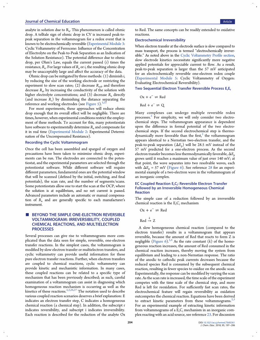
analyte in solution due to Ru. This phenomenon is called ohmicdrop. A telltale sign of ohmic drop in CV is increased peak-to-peak separation in the voltammogram for a redox event that isknown to be electrochemically reversible (Experimental Module 3:Cyclic Voltammetry of Ferrocene: Influence of the Concentrationof Electrolyte on the Peak-to-Peak Separation as an Indication ofthe Solution Resistance). The potential difference due to ohmicdrop, per Ohm’s Law, equals the current passed (i) times theresistance, Ru. For large values of Ru or i, the resulting ohmic dropmay be unacceptably large and affect the accuracy of the data.Ohmic drop can bemitigated by threemethods: (1) diminish i,

by reducing the size of the working electrode or restricting theexperiment to slow scan rates; (2) decrease Rsol, and thereforedecrease Ru, by increasing the conductivity of the solution withhigher electrolyte concentrations; and (3) decrease Ru directly(and increase Rc) by diminishing the distance separating thereference and working electrodes (see Figure 5).3,25

For most experiments, these approaches will reduce ohmicdrop enough that its overall effect will be negligible. There aretimes, however, when experimental conditions restrict the employ-ment of these methods. To account for this, many potentiostatshave software to experimentally determine Ru and compensate forit in real time (Experimental Module 2: Experimental Determi-nation of the Uncompensated Resistance).

Recording the Cyclic Voltammogram

Once the cell has been assembled and sparged of oxygen andprecautions have been taken to minimize ohmic drop, experi-ments can be run. The electrodes are connected to the poten-tiostat, and the experimental parameters are selected through thepotentiostat software. While different software will requiredifferent parameters, fundamental ones are the potential windowthat will be scanned (defined by the initial, switching, and finalpotentials), the scan rate, and the number of segments/scans.Some potentiostats allow one to start the scan at the OCP, wherethe solution is at equilibrium, and no net current is passed.Advanced parameters include an automatic or manual compensa-tion of Ru and are generally specific to each manufacturer’sinstrument.

■ BEYOND THE SIMPLE ONE-ELECTRON REVERSIBLEVOLTAMMOGRAM: IRREVERSIBILITY, COUPLEDCHEMICAL REACTIONS, AND MULTIELECTRONPROCESSES

Several processes can give rise to voltammograms more com-plicated than the data seen for simple, reversible, one-electrontransfer reactions. In the simplest cases, the voltammogram ismodified by slow electron transfer or multielectron transfers, andcyclic voltammetry can provide useful information for thesepure electron transfer reactions. Further, when electron transfersare coupled to chemical reactions, cyclic voltammetry canprovide kinetic and mechanistic information. In many cases,these coupled reactions can be related to a specific type ofmechanism that has been previously described; as such, carefulexamination of a voltammogram can assist in diagnosing whichhomogeneous reaction mechanism is occurring as well as thekinetics of these reactions.2,3,26,27 The notation used to describevarious coupled reaction scenarios deserves a brief explanation: Eindicates an electron transfer step, C indicates a homogeneouschemical reaction (a chemical step). In addition, the subscript rindicates reversibility, and subscript i indicates irreversibility.Each reaction is described for the reduction of the analyte Ox

to Red. The same concepts can be readily extended to oxidativereactions.Electrochemical Irreversibility

When electron transfer at the electrode surface is slow compared tomass transport, the process is termed “electrochemically irrever-sible.” As noted above in the Cyclic Voltammetry Profile section,slow electrode kinetics necessitate significantly more negativeapplied potentials for appreciable current to flow. As a result,peak-to-peak separation is larger than the 57 mV anticipatedfor an electrochemically reversible one-electron redox couple(Experimental Module 5: Cyclic Voltammetry of Oxygen:Evaluating Electrochemical Reversibility).Two Sequential Electron Transfer Reversible Process ErEr

+ ⇌−Ox e Red

+ ⇌−Red e Q

Many complexes can undergo multiple reversible redoxprocesses.2 For simplicity, we will only consider two electro-chemical steps. The voltammogram appearance is dependentupon the difference in formal potential of the two electro-chemical steps. If the second electrochemical step is thermo-dynamically more favorable than the first,2 the voltammogramappears identical to a Nernstian two-electron transfer, and thepeak-to-peak separation (ΔEp) will be 28.5 mV instead of the57 mV predicted for a one-electron process. As the secondelectron transfer becomes less thermodynamically favorable,ΔEpgrows until it reaches a maximum value of just over 140 mV; atthat point, the wave separates into two resolvable waves, eachwith ΔEp = 57 mV (Figure 6). See reference 28 for an experi-mental example of a two-electron wave in the voltammogram ofan inorganic complex.

EC Coupled Reaction ErCi: Reversible Electron TransferFollowed by an Irreversible Homogeneous ChemicalReaction

The simple case of a reduction followed by an irreversiblechemical reaction is the ErCi mechanism

+ ⇌−Ox e Red

→Red Zk

A slow homogeneous chemical reaction (compared to theelectron transfer) results in a voltammogram that appearsreversible, because the amount of Red that reacts to form Z isnegligible (Figure 6).2,4 As the rate constant (k) of the homo-geneous reaction increases, the amount of Red consumed in thechemical reaction increases, thereby moving the system fromequilibrium and leading to a non-Nernstian response. The ratioof the anodic to cathodic peak currents decreases because thereduced species Red is consumed by the subsequent chemicalreaction, resulting in fewer species to oxidize on the anodic scan.Experimentally, the response can be modified by varying the scanrate. As the scan rate is increased, the time scale of the experimentcompetes with the time scale of the chemical step, and moreRed is left for reoxidation. For sufficiently fast scan rates, theelectrochemical feature will regain reversibility as oxidationoutcompetes the chemical reaction. Equations have been derivedto extract kinetic parameters from these voltammograms.2,3

For an experimental example of extracting kinetic informationfrom voltammograms of a ErCi mechanism in an inorganic com-plex reacting with an acid source, see reference 23. For discussion



204





on using this methodology to estimate rates of intramoleculardecomposition upon reduction/oxidation, see reference 29.CE Coupled Reaction CrEr: Reversible Chemical StepFollowed by a Reversible Electron Transfer

Another simple case is the CrEr mechanism

⇌Z Ox

+ ⇌−Ox e RedIn this example, the amount of Ox available for the reduction is

dictated by the equilibrium constant of the first step. The greaterthe equilibrium constant, the more reversible the voltammogram(Figure 6). In the extreme case where the equilibrium constantis so large as to be considered an irreversible reaction, thevoltammogram becomes completely reversible. The equilibriumconstant can be extracted from voltammograms in certain cases.2,3,30

■ CONCLUSIONQuantitative electrochemical analysis is a powerful tool forexploring the electron transfer reactions underpinning renewableenergy technologies and fundamental mechanistic inorganicchemistry. Increasingly, emerging investigators are interested inutilizing electrochemistry to advance their research. Through

this tutorial, we have aimed to provide these researchers withan approachable and comprehensive guide to utilizing cyclicvoltammetry in research and education endeavors. By integratingthe theoretical underpinnings of electrochemical analysis withpractical experimental details, highlighting experimental pitfalls,and providing introductory training modules, this text reflectscurrent best practices in learning and utilizing cyclic voltammetry.

■ ASSOCIATED CONTENT*S Supporting Information

The Supporting Information is available on the ACS Publicationswebsite at DOI: 10.1021/acs.jchemed.7b00361.

All modules mentioned in the text (PDF, DOCX)

■ AUTHOR INFORMATIONCorresponding Author

*E-mail: [email protected].

ORCID

Noemie Elgrishi: 0000-0001-9776-5031Jillian L. Dempsey: 0000-0002-9459-4166Notes

The authors declare no competing financial interest.

■ ACKNOWLEDGMENTSWe thank current and past group members who tested thetraining modules: Will Howland, Tao Huang, Carolyn Hartley,Banu Kandemir, Daniel Kurtz, Katherine Lee, Emily AnneSharpe, and Hannah Starr. N.E. thanks Brian Lindley for helpfuldiscussions. J.L.D. thanks AaronWilson and Xile Hu as well as allof the Cyclic Voltammetry International School (CVIS)instructors: Cedric Tard, Cyrille Costentin, Marc Robert, andJean-Michel Saveant, for insightful discussions. We also thankPine Research Instrumentation for assistance with the method todetermine cell resistance. This work was supported by the U.S.Department of Energy, Office of Science, Office of Basic EnergySciences, under Award DE-SC0015303 and the University ofNorth Carolina at Chapel Hill.

■ REFERENCES(1) Zoski, C. G., Ed. Handbook of Electrochemistry; Elsevier:Amsterdam, The Netherlands, 2006.(2) Bard, A. J.; Faulkner, L. R. Electrochemical Methods: Fundamentaland Applications, 2nd ed.; John Wiley & Sons: Hoboken, NJ, 2001.(3) Saveant, J.-M. Elements of Molecular and Biomolecular Electro-chemistry; John Wiley & Sons: Hoboken, NJ, 2006.(4) Compton, R. G.; Banks, C. E. Understanding Voltammetry, 2nd ed.;Imperial College Press: London, U.K., 2011.(5) Graham, D. J. Standard Operating Procedures for Cyclic Voltammetry.https://sop4cv.com/index.html (accessed Jun 2017).(6) Ventura, K.; Smith, M. B.; Prat, J. R.; Echegoyen, L. E.; Villagran, D.Introducing Students to Inner Sphere Electron Transfer Conceptsthrough Electrochemistry Studies in Diferrocene Mixed-ValenceSystems. J. Chem. Educ. 2017, 94 (4), 526−529.(7) Hendel, S. J.; Young, E. R. Introduction to Electrochemistry andthe Use of Electrochemistry to Synthesize and Evaluate Catalysts forWater Oxidation and Reduction. J. Chem. Educ. 2016, 93 (11), 1951−1956.(8) Baca, G.; Dennis, A. L. Electrochemistry in a Nutshell A GeneralChemistry Experiment. J. Chem. Educ. 1978, 55 (12), 804.(9) Faulkner, L. R. Understanding Electrochemistry: Some DistinctiveConcepts. J. Chem. Educ. 1983, 60 (4), 262.

Figure 6. Examples of voltammograms modeled using DigiElchsimulation software for three common mechanisms. The currents arenormalized. ErCi mechanism: increasing the scan rate (from υ = 0.1 (red)to 1 (green) to 10 V s−1 (blue)) restores reversibility (rate constant for theCi step k = 5 s

−1). CrEr mechanism: the faster the forward rate constant ofthe Cr step, the more reversible the voltammogram (Keq = 0.1, kf = 1(blue), 10 (dark green), 100 (lime green), 1000 s−1 (red)). ErErmechanism: as the separations between the two reduction potentials(ΔE1/2) decreases, the peaks merge to become a single two-electron peak.ΔE1/2 = −0.05 (dark blue), 0 (light blue), 0.05 (dark green), 0.1 (limegreen), 0.15 (orange), and 0.2 V (red).



205

http://pubs.acs.org

http://pubs.acs.org

http://pubs.acs.org/doi/abs/10.1021/acs.jchemed.7b00361


http://pubs.acs.org/doi/suppl/10.1021/acs.jchemed.7b00361/suppl_file/ed7b00361_si_002.docx

mailto:[email protected]

http://orcid.org/0000-0001-9776-5031

http://orcid.org/0000-0002-9459-4166

https://sop4cv.com/index.html


(10) Moran, P. J.; Gileadi, E. Alleviating the Common ConfusionCaused by Polarity in Electrochemistry. J. Chem. Educ. 1989, 66 (11),912.(11) Birss, V. I.; Truax, D. R. An Effective Approach to TeachingElectrochemistry. J. Chem. Educ. 1990, 67 (5), 403.(12) Connelly, N. G.; Geiger, W. E. Chemical Redox Agents forOrganometallic Chemistry. Chem. Rev. 1996, 96 (2), 877−910.(13) Mabbott, G. A. An Introduction to Cyclic Voltammetry. J. Chem.Educ. 1983, 60 (9), 697−702.(14) Izutsu, K. Electrochemistry in Nonaqueous Solutions; Wiley-VCH:Weinheim, Germany, 2003.(15) Kissinger, P. T.; Heineman, W. R. Cyclic Voltammetry. J. Chem.Educ. 1983, 60, 702−706.(16) The effective concentration of a species in nonideal conditions iscalled the activity. It corresponds to the effective chemical potential of asolution, rather than an ideal one.(17) Ranganathan, S.; Kuo, T.-C.; McCreery, R. L. Facile Preparationof Active Glassy Carbon Electrodes with Activated Carbon and OrganicSolvents. Anal. Chem. 1999, 71 (16), 3574−3580.(18) McCarthy, B. D.; Martin, D. J.; Rountree, E. S.; Ullman, A. C.;Dempsey, J. L. Electrochemical Reduction of Brønsted Acids by GlassyCarbon in AcetonitrileImplications for Electrocatalytic HydrogenEvolution. Inorg. Chem. 2014, 53 (16), 8350−8361.(19) Pavlishchuk, V. V.; Addison, A. W. Conversion Constants forRedox Potentials Measured versus Different Reference Electrodes inAcetonitrile Solutions at 25°C. Inorg. Chim. Acta 2000, 298 (1), 97−102.(20) Gagne, R. R.; Koval, C. A.; Lisensky, G. C. Ferrocene as anInternal Standard for Electrochemical Measurements. Inorg. Chem.1980, 19 (9), 2854−2855.(21) Trasatti, S. The Absolute Electrode Potential: An ExplanatoryNote (Recommendations 1986). Pure Appl. Chem. 1986, 58 (7), 955−966.(22) Aranzaes, J. R.; Daniel, M.-C.; Astruc, D. Metallocenes asReferences for the Determination of Redox Potentials by CyclicVoltammetryPermethylated Iron and Cobalt Sandwich Complexes,Inhibition by Polyamine Dendrimers, and the Role of Hydroxy-Containing Ferrocenes. Can. J. Chem. 2006, 84 (2), 288−299.(23) Elgrishi, N.; Kurtz, D. A.; Dempsey, J. L. Reaction ParametersInfluencing Cobalt Hydride Formation Kinetics: Implications forBenchmarking H2-Evolution Catalysts. J. Am. Chem. Soc. 2017, 139(1), 239−244.(24) Myland, J. C.; Oldham, K. B. Uncompensated Resistance. 1. TheEffect of Cell Geometry. Anal. Chem. 2000, 72 (17), 3972−3980.(25) Oldham, K. B.; Stevens, N. P. C. Uncompensated Resistance. 2.The Effect of Reference Electrode Nonideality. Anal. Chem. 2000, 72(17), 3981−3988.(26) Elgrishi, N.; McCarthy, B. D.; Rountree, E. S.; Dempsey, J. L.Reaction Pathways of Hydrogen-Evolving Electrocatalysts: Electro-chemical and Spectroscopic Studies of Proton-Coupled ElectronTransfer Processes. ACS Catal. 2016, 6 (6), 3644−3659.(27) Lee, K. J.; Elgrishi, N.; Kandemir, B.; Dempsey, J. L.Electrochemical and Spectroscopic Methods for Evaluating MolecularElectrocatalysts. Nat. Rev. Chem. 2017, 1 (5), 0039.(28) Sampson, M. D.; Nguyen, A. D.; Grice, K. A.; Moore, C. E.;Rheingold, A. L.; Kubiak, C. P. Manganese Catalysts with BulkyBipyridine Ligands for the Electrocatalytic Reduction of CarbonDioxide: Eliminating Dimerization and Altering Catalysis. J. Am.Chem. Soc. 2014, 136 (14), 5460−5471.(29) Nicholson, R. S. Semiempirical Procedure for Measuring withStationary Electrode Polarography Rates of Chemical ReactionsInvolving the Product of Electron Transfer. Anal. Chem. 1966, 38(10), 1406.(30) Saveant, J. M.; Xu, F. First- and Second-Order Chemical-Electrochemical Mechanisms: Extraction of Standard Potential,Equilibrium and Rate Constants from Linear Sweep VoltammetricCurves. J. Electroanal. Chem. Interfacial Electrochem. 1986, 208 (2), 197−217.



206


Cyclic Voltammetry

Denis Andrienko

January 22, 2008

2

Literature:

1. Allen J. Bard, Larry R. Faulkner “Electrochemical Methods: Fundamentals and Applications”

2. http://www.cheng.cam.ac.uk/research/groups/electrochem/teaching.html

Chapter 1

Cyclic Voltammetry

1.1 Background

Cyclic voltammetry is the most widely used technique for acquiring qualitative information about elec-trochemical reactions. it offers a rapid location of redox potentials of the electroactive species.

A few concepts has to be introduced before talking about this method.

1.1.1 Electronegativity

Electronegativity is the affinity for electrons. The atoms of the various elements differ in their affinity forelectrons. The term was first proposed by Linus Pauling in 1932 as a development of valence bond theory.The table for all elements can be looked up on Wikipedia: http://en.wikipedia.org/wiki/Electronegativity.

Some facts to remember:

• Fluorine (F) is the most electronegative element. χF = 3.98.

• The electronegativity of oxygen (O) χO = 3.44 is exploited by life, via shuttling of electrons betweencarbon (C, χF = 2.55) and oxygen (O): Moving electrons against the gradient (O to C) - as occursin photosynthesis - requires energy (and stores it). Moving electrons down the gradient (C to O) -as occurs in cellular respiration - releases energy.

• The relative electronegativity of two interacting atoms plays a major part in determining what kindof chemical bond forms between them.

Examples:

• Sodium (χNa = 0.93) and Chlorine (χCl = 3.16) = Ionic Bond: There is a large difference inelectronegativity, so the chlorine atom takes an electron from the sodium atom converting theatoms into ions (Na+) and (Cl−). These are held together by their opposite electrical chargeforming ionic bonds. Each sodium ion is held by 6 chloride ions while each chloride ion is, in turn,held by 6 sodium ions. Result: a crystal lattice (not molecules) of common table salt (NaCl).

• Carbon (C) and Oxygen (O) = Covalent Bond. There is only a small difference in electronegativity,so the two atoms share the electrons. a covalent bond (depicted as C:H or C-H) is formed, whereatoms are held together by the mutual affinity for their shared electrons. An array of atoms heldtogether by covalent bonds forms a true molecule.

• Hydrogen (H) and Oxygen (O) = Polar Covalent Bond. Moderate difference in electronegativity,oxygen atom pulls the electron of the hydrogen atom closer to itself. Result: a polar covalent bond.Oxygen does this with 2 hydrogen atoms to form a molecule of water.

Molecules, like water, with polar covalent bonds are themselves polar; that is, have partial electricalcharges across the molecule; may be attracted to each other (as occurs with water molecules); are goodsolvents for polar and/or hydrophilic compounds. May form hydrogen bonds.

3

4 CHAPTER 1. CYCLIC VOLTAMMETRY

1.2 Electrode Reactions

A typical electrode reaction involves the transfer of charge between an electrode and a species in solution.The electrode reaction usually referred to as electrolysis, typically involves a series of steps:

1. Reactant (O) moves to the interface: this is termed mass transport

2. Electron transfer can then occur via quantum mechanical tunnelling between the electrode andreactant close to the electrode (typical tunnelling distances are less than 2 nm)

3. The product (R) moves away from the electrode to allow fresh reactant to the surface

The ‘simplest’ example of an electrode reaction is a single electron transfer reaction, e.g. Fe3+ +e− =Fe2+. Several examples are shown in Fig. 1.1

Figure 1.1: Simple electrode reactions: (left) A single electron transfer reaction. Here the reactantFe3+ moves to the interface where it undergoes a one electron reduction to form Fe2+. The electron issupplied via the electrode which is part of a more elaborate electrical circuit. For every Fe3+ reduceda single electron must flow. By keeping track of the number of electrons flowing (ie the current) it ispossible to say exactly how many Fe3+ molecules have been reduced. (middle) Copper deposition at aCu electrode. In this case the electrode reaction results in the fomation of a thin film on the orginalsurface. It is possible to build up multiple layers of thin metal films simply by passing current throughappropriate reactant solutions. (right) Electron transfer followed by chemical reaction. In this case anorganic molecule is reduced at the electrode forming the radical anion. This species however is unstableand undergoes further electrode and chemical reactions.

1.3 Electron Transfer and Energy levels

The key to driving an electrode reaction is the application of a voltage. If we consider the units of volts

V = Joule/Coulomb (1.1)

we can see that a volt is simply the energy required to move charge. Application of a voltage to anelectrode therefore supplies electrical energy. Since electrons possess charge an applied voltage can alterthe ’energy’ of the electrons within a metal electrode. The behaviour of electrons in a metal can bepartly understood by considering the Fermi-level. Metals are comprised of closely packed atoms whichhave strong overlap between one another. A piece of metal therefore does not possess individual welldefined electron energy levels that would be found in a single atom of the same material. Instead acontinum of levels are created with the available electrons filling the states from the bottom upwards.The Fermi-level corresponds to the energy at which the ’top’ electrons sit.

1.4. KINETICS OF ELECTRON TRANSFER 5

Figure 1.2: Representation of the Fermi-Level in a metal at three different applied voltages (left).Schematic representation of the reduction of a species (O) in solution (right).

This level is not fixed and can be moved by supplying electrical energy. Electrochemists are thereforeable to alter the energy of the Fermi-level by applying a voltage to an electrode.

Figure 1.2 shows the Fermi-level within a metal along with the orbital energies (HOMO and LUMO)of a molecule (O) in solution. On the left hand side the Fermi-level has a lower value than the LUMOof (O). It is therefore thermodynamically unfavourable for an electron to jump from the electrode tothe molecule. However on the right hand side, the Fermi-level is above the LUMO of (O), now it isthermodynamically favourable for the electron transfer to occur, ie the reduction of O.

Whether the process occurs depends upon the rate (kinetics) of the electron transfer reaction and thenext document describes a model which explains this behavior.

1.4 Kinetics of Electron Transfer

In this section we will develop a quantitative model for the influence of the electrode voltage on the rateof electron transfer. For simplicity we will consider a single electron transfer reaction between two species(O) and (R)

O + e− kred−−→ R (1.2)

Rkox−−→ O + e− (1.3)

The current flowing in either the reductive or oxidative steps can be predicted using the followingexpressions

iO = FAkoxcR (1.4)iR = −FAkredcO (1.5)

For the reduction reaction the current iR is related to the electrode area A, the surface concentrationof the reactant cO, the rate constant for the electron transfer kred and Faraday’s constant F . A similarexpression is valid for the oxidation, now the current is labelled iO, with the surface concentration that ofthe species R. Similarly the rate constant for electron transfer corresponds to that of the oxidation process.Note that by definition the reductive current is negative and the oxidative positive, the difference in signsimply tells us that current flows in opposite directions across the interface depending upon whether weare studying an oxidation or reduction. To establish how the rate constants kox and kred are influencedby the applied voltage we will use transition state theory.

In this theory the reaction is considered to proceed via an energy barrier, as shown in Fig 1.3. Thesummit of this barrier is referred to as the transition state. Using this picture the corresponding reactionrates are given by

kred,ox = Z exp(−∆Gred,ox

kBT

)(1.6)

If we plot a series of the free energy profiles as a function of voltage the free energy of R will beinvariant with voltage, whereas the right handside (O + e) shows a strong dependence.


Figure 1.3: Transition occurs via a barrier ∆G.

This can be explained in terms of the Fermi level diagrams noted earlier: as the voltage is altered theFermi level is raised (or lowered) changing the energy state of the electrons.

However it is not just the thermodynamic aspects of the reaction that can be influenced by thisvoltage change as the overall barrier height (ie activation energy) can also be seen to alter as a functionof the applied voltage. We might therefore predict that the rate constants for the forward and reversereactions will be altered by the applied voltage. In order to formulate a model we will assume that theeffect of voltage on the free energy change will follow a linear relationship (this is undoubtedly an oversimplification). Using this linear relationship the activation free energies for reduction and oxidation willvary as a function of the applied voltage as follows (Buttler-Volmer model)

∆Gred = ∆Gred(V = 0) + αFV (1.7)∆Gox = ∆Gox(V = 0)− (1− α)FV (1.8)

The parameter α is called the transfer coefficient and typically is found to have a value of 0.5.Physically it provides an insight into the way the transition state is influenced by the voltage. A value ofone half means that the transition state behaves mid way between the reactants and products response toapplied voltage. The free energy on the right hand side of both of the above equations can be consideredas the chemical component of the activation free energy change, ie it is only dependent upon the chemicalspecies and not the applied voltage. We can now substitute the activation free energy terms above intothe expressions for the oxidation and reduction rate constants, which gives

kred = Z exp−∆GV =0

red

kBTexp

−αFV

kBT(1.9)

kox = Z exp−∆GV =0

ox

kBTexp

(1− α)FV

kBT(1.10)

These results show us the that rate constants for the electron transfer steps are proportional to theexponential of the applied voltage. So the rate of electrolysis can be changed simply by varying the appliedvoltage. This result provides the fundamental basis of the experimental technique called voltammetrywhich we will look at more closely later.

In conclusion we have seen that the rate of electron transfer can be influenced by the applied voltageand it is found experimentally that this behaviour can be quantified well using the simple model presentedabove. However the kinetics of the electron transfer is not the only process which can control theelectrolysis reaction. In many circumstances it is the rate of transport to the electrode which controlsthe overall reaction.

1.5 Mass transport

In the electrode kinetics section we have seen that the rate of reaction can be influenced by the cellpotential difference. However, the rate of transport to the surface can also effect or even dominate theoverall reaction rate and in this section we look at the different forms of mass transport that can influenceelectrolysis reactions.

1.5. MASS TRANSPORT 7

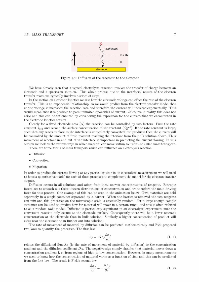
Figure 1.4: Diffusion of the reactants to the electrode

We have already seen that a typical electrolysis reaction involves the transfer of charge between anelectrode and a species in solution. This whole process due to the interfacial nature of the electrontransfer reactions typically involves a series of steps.

In the section on electrode kinetics we saw how the electrode voltage can effect the rate of the electrontransfer. This is an exponential relationship, so we would predict from the electron transfer model thatas the voltage is increased the reaction rate and therefore the current will increase exponentially. Thiswould mean that it is possible to pass unlimited quantities of current. Of course in reality this does notarise and this can be rationalized by considering the expression for the current that we encountered inthe electrode kinetics section

Clearly for a fixed electrode area (A) the reaction can be controlled by two factors. First the rateconstant kred and second the surface concentration of the reactant (Csurf

O ). If the rate constant is large,such that any reactant close to the interface is immediately converted into products then the current willbe controlled by the amount of fresh reactant reaching the interface from the bulk solution above. Thusmovement of reactant in and out of the interface is important in predicting the current flowing. In thissection we look at the various ways in which material can move within solution - so called mass transport.

There are three forms of mass transport which can influence an electrolysis reaction

• Diffusion

• Convection

• Migration

In order to predict the current flowing at any particular time in an electrolysis measurement we will needto have a quantitative model for each of these processes to complement the model for the electron transferstep(s).

Diffusion occurs in all solutions and arises from local uneven concentrations of reagents. Entropicforces act to smooth out these uneven distributions of concentration and are therefore the main drivingforce for this process. One example of this can be seen in the animation below. Two materials are heldseparately in a single container separated by a barrier. When the barrier is removed the two reagentscan mix and this processes on the microscopic scale is essentially random. For a large enough samplestatistics can be used to predict how far material will move in a certain time - and this is often referredto as a random walk model. Diffusion is particularly significant in an electrolysis experiment since theconversion reaction only occurs at the electrode surface. Consequently there will be a lower reactantconcentration at the electrode than in bulk solution. Similarly a higher concentration of product willexist near the electrode than further out into solution.

The rate of movement of material by diffusion can be predicted mathematically and Fick proposedtwo laws to quantify the processes. The first law

JO = −DO∂cO

∂x(1.11)

relates the diffusional flux JO (ie the rate of movement of material by diffusion) to the concentrationgradient and the diffusion coefficient DO. The negative sign simply signifies that material moves down aconcentration gradient i. e. from regions of high to low concentration. However, in many measurementswe need to know how the concentration of material varies as a function of time and this can be predictedfrom the first law. The result is Fick’s second law

∂cO

∂t= −∂JO

∂x(1.12)


Figure 1.5: Schematic of the setup.

In this case we consider diffusion normal to an electrode surface (x direction). The rate of change of theconcentration cO as a function of time t can be seen to be related to the change in the concentrationgradient. So the steeper the change in concentration the greater the rate of diffusion. In practice diffusionis often found to be the most significant transport process for many electrolysis reactions.

Fick’s second law is an important relationship since it permits the prediction of the variation ofconcentration of different species as a function of time within the electrochemical cell. In order to solvethese expressions analytical or computational models are usually employed.

1.6 Voltammetry

Voltammetry is one of the techniques which electrochemists employ to investigate electrolysis mechanisms.There are numerous forms of voltammetry

• Potential Step

• Linear sweep

• Cyclic Voltammetry

For each of these cases a voltage or series of voltages are applied to the electrode and the correspondingcurrent that flows monitored. In this section we will examine potential step voltammetry, the other formsare described on separate pages

For the moment we will focus on voltammetry in stagnant solution. The figure below shows a schematicof an electrolysis cell. There is a working electrode which is hooked up to an external electrical circuit.For our purposes at the moment we will not worry about the remainder of the circuit, obviously theremust be more than one electrode for current to flow. But as we shall see later it is only the so calledworking electrode that controls the flow of current flow in the electrochemical measurement. The essentialelements needed for an electolysis measurement are as follows:

• The electrode: This is usually made of an inert metal (such as Gold or Platinum)

• The solvent: This usually has a high dielectric constant (eg water or acetonitrile) to enable theelectrolyte to dissolve and help aid the passage of current.

• A background electrolyte: This is an electrochemically inert salt (eg NaCl or Tetra butylammoniumperchlorate, TBAP) and is usually added in high concentration (0.1M) to allow the current to pass.

• The reactant: Typically in low concentration 10−3 M.

1.6.1 Potential Step Voltammetry

In the potential step measurement the applied voltage is instantaneously jumped from one value V1 toanother V2 The resulting current is then measured as a function time. If we consider the reaction

Fe3+(s) + e− kred−−→ Fe2+(s) (1.13)

1.7. LINEAR SWEEP VOLTAMMETRY 9

Figure 1.6: Potential step voltammetry: voltage vs time, current versus voltage, and concentration versusdistance from the electrode plotted for several times.

Figure 1.7: Linear increase of the potential vs time.

Usually the voltage range is set such that at V1 the reduction of (Fe3+ ) is thermodynamically unfavorable.The second value of voltage (V2) is selected so that any Fe3+ close to the electrode surface is convertedto product (Fe2+). Under these conditions the current response is in Fig. 1.6.1

The current rises instantaneously after the change in voltage and then begins to drop as a functionof time. This occurs since the instant before the voltage step the surface of the electrode is completelycovered in the reactant and the solution has a constant composition below

Once the step occurs reactant (Fe3+ is converted to product Fe2+ and a large current begins to flow.However now for the reaction to continue we need a supply of fresh reactant to approach the electrodesurface. This happens in stagnant solution via diffusion. As we noted in a previous section the rate ofdiffusion is controlled by the concentration gradient. So the supply of fresh Fe3+ to the surface (andtherefore the current flowing) depends upon the diffusional flux. At short times the diffusional flux ofFe3+ is high, as the change in concentration between the bulk value and that at the surface occurs overa short distance

As the electrolysis continues material can diffuse further from the electrode and therefore the concen-tration gradient drops. As the concentration gradient drops (see concentration profiles below) so doesthe supply of fresh reactant to the surface and therefore the current also decreases.

Solving the mass transport equation in 1D case we obtain

i = nFAkredcbulkO

√D

πt∝ t−1/2 (1.14)

Here the current is related to the bulk reactant concentration. Step voltammetry allows the estimationof the diffusion coefficients of the species to be obtained.

1.7 Linear Sweep Voltammetry

In linear sweep voltammetry (LSV) a fixed potential range is employed much like potential step measure-ments. However in LSV the voltage is scanned from a lower limit to an upper limit as shown below. Thecharacteristics of the linear sweep voltammogram depend on a number of factors including:


Figure 1.8: Linear increase of the potential vs time.

• The rate of the electron transfer reaction(s)

• The chemical reactivity of the electroactive species

• The voltage scan rate

In LSV measurements the current response is plotted as a function of voltage rather than time, unlikepotential step measurements.

The scan begins from the left hand side of the current/voltage plot where no current flows. As thevoltage is swept further to the right (to more reductive values) a current begins to flow and eventuallyreaches a peak before dropping. To rationalise this behaviour we need to consider the influence of voltageon the equilibrium established at the electrode surface. Here the rate of electron transfer is fast incomparsion to the voltage sweep rate. Therefore at the electrode surface an equilibrum is establishedidentical to that predicted by thermodynamics. You may recall from equilibrium electrochemistry thatthe Nernst equation

The exact form of the voltammogram can be rationalised by considering the voltage and mass transporteffects. As the voltage is initially swept from V1 the equilibrium at the surface begins to alter and thecurrent begins to flow. The current rises as the voltage is swept further from its initial value as theequilibrium position is shifted further to the right hand side, thus converting more reactant. The peakoccurs, since at some point the diffusion layer has grown sufficiently above the electrode so that the fluxof reactant to the electrode is not fast enough to satisfy that required by the Nernst equation. In thissituation the curent begins to drop just as it did in the potential step measurements. In fact the drop incurrent follows the same behaviour as that predicted by the Cottrell equation.

The above voltammogram was recorded at a single scan rate. If the scan rate is altered the currentresponse also changes. The figure 1.8 shows a series of linear sweep voltammograms recorded at differentscan rates. Each curve has the same form but it is apparent that the total current increases with increasingscan rate. This again can be rationalised by considering the size of the diffusion layer and the time takento record the scan. Clearly the linear sweep voltammogram will take longer to record as the scan rate isdecreased. Therefore the size of the diffusion layer above the electrode surface will be different dependingupon the voltage scan rate used. In a slow voltage scan the diffusion layer will grow much further fromthe electrode in comparison to a fast scan. Consequently the flux to the electrode surface is considerablysmaller at slow scan rates than it is at faster rates. As the current is proportional to the flux towards theelectrode the magnitude of the current will be lower at slow scan rates and higher at high rates. Thishighlights an important point when examining LSV (and cyclic voltammograms), although there is notime axis on the graph the voltage scan rate (and therefore the time taken to record the voltammogram)do strongly effect the behaviour seen. A final point to note from the figure is the position of the currentmaximum, it is clear that the peak occurs at the same voltage and this is a characteristic of electrodereactions which have rapid electron transfer kinetics. These rapid processes are often referred to asreversible electron transfer reactions.

This leaves the question as to what would happen if the electron transfer processes were ‘slow’ (relativeto the voltage scan rate). For these cases the reactions are referred to as quasi-reversible or irreversible

1.7. LINEAR SWEEP VOLTAMMETRY 11

Figure 1.9: Change of the rate constant.

Figure 1.10: Voltage as a function of time and current as a function of voltage for CV

electron transfer reactions. The figure below shows a series of voltammograms recorded at a single voltagesweep rate for different values of the reduction rate constant kred

In this situation the voltage applied will not result in the generation of the concentrations at theelectrode surface predicted by the Nernst equation. This happens because the kinetics of the reactionare ’slow’ and thus the equilibria are not established rapidly (in comparison to the voltage scan rate).In this situation the overall form of the voltammogram recorded is similar to that above, but unlike thereversible reaction now the position of the current maximum shifts depending upon the reduction rateconstant (and also the voltage scan rate). This occurs because the current takes more time to respondto the the applied voltage than the reversible case.

1.7.1 Cyclic Voltammetry

Cyclic voltammetry (CV) is very similar to LSV. In this case the voltage is swept between two values(see below) at a fixed rate, however now when the voltage reaches V2 the scan is reversed and the voltageis swept back to V1

A typical cyclic voltammogram recorded for a reversible single electrode transfer reaction is shown inbelow. Again the solution contains only a single electrochemical reactant

The forward sweep produces an identical response to that seen for the LSV experiment. When thescan is reversed we simply move back through the equilibrium positions gradually converting electrolysisproduct (Fe2+ back to reactant (Fe3+. The current flow is now from the solution species back to theelectrode and so occurs in the opposite sense to the forward seep but otherwise the behaviour can beexplained in an identical manner. For a reversible electrochemical reaction the CV recorded has certainwell defined characteristics.

1. The voltage separation between the current peaks is

2. The positions of peak voltage do not alter as a function of voltage scan rate


Figure 1.11: Scan rate and rate constant dependence of the I-V curves.

3. The ratio of the peak currents is equal to one

4. The peak currents are proportional to the square root of the scan rate

The influence of the voltage scan rate on the current for a reversible electron transfer can be seen inFig. 1.11 As with LSV the influence of scan rate is explained for a reversible electron transfer reactionin terms of the diffusion layer thickness. The CV for cases where the electron transfer is not reversibleshow considerably different behaviour from their reversible counterparts.

By analysing the variation of peak position as a function of scan rate it is possible to gain an estimatefor the electron transfer rate constants.

CYCLIC Voltammetry

⇒ read more: C.M.A. Brett & A.M.O. Brett, “Electrochemistry”,

Oxford University Press, Oxford, 1993 chapter 9 →

E. Gileadi, “Electrode Kinetics for Chemists, Chemical Engineers and Materials Scientists”, VCH, Weinheim, 1993 → chapter 25

Lecture Notes : http://www.sfu.ca/~aroudgar/Tutorials/lecture27-31.pdf

Different ways to do voltammetry: Potential step Linear sweep Cyclic Voltammetry (CV)

CV: widely used technique for studying electrode processes (particularly by non-electrochemists)

Principle of CV: Apply continuous cyclic potential E to working electrode

⇒ Effects Faradic reactions: oxidation/reduction of

electroactive species in solution Adsorption/desorption due to E Capacitive current: double layer charging

⇒ deviations from steady state, i.e.dd

0ct≠

mass transport

vs.

kinetics

t j vs.j E

CV: lane pj E t− −

Potential changed at a constant sweep rate, ddEvt

=

Cycled forward and backward between fixed values Current plotted as a function of potential

t

E

Emax

Emin

EiEf

In principle: useful… Unknown electrochemical system

→ start analysis with CV → survey over processes, kinetics → identify involved species and mechanisms

qualitative understanding ⇒

Semi-quantitative analysis

→ diagnostic capabilities … but difficult to understand and analyze

→ a lot of information → difficult to discern!!!

How do typical cyclic voltammograms look like?

Measured Current

→ total current density:

F C

F ddd

j j jEj Ct

= +

= +

v

→→→

faradaic current + capacitive current

electrode reaction double layer charging

F dj j vC= +

rate constants double layer correction Double layer correction important if is large!

What do we need?

Nernst-equation equilibrium

Butler-Volmer equation kinetics

Diffusion equation mass transport Double layer charging Adsorption

⇒ anything new??

What is controlled in CV? Variation of applied potential with time

t

E

Emax

Emin

EiEf

Important parameters:

iE Initial potential ,

Initial sweep direction

solvent

stability

~ mV s-1 103-104 V s-1to Sweep rate, -1 [mV s ]v

maxE

min

Maximum potential,

E Minimum potential,

fE Final potential,

Sweep rate: 3 ranges of operation (1) very slow sweeps ( nothing new!) →

-1mV s0.1 2v = −

-1 V s0.01 100v = −

quasi-steady state conditions sweep rate and reversal: no effect on j/E relationship

corrosion passivation fuel cell reactions

(2) Oxidation or reduction of species in the bulk

measurement time (10-50 s)(mass transport)

• double layer charging• uncompensated

solution resistance

(3) Oxidation/reduction of species on surface

-1 V s0.01 100v = −

background currents, impurities

• double layer charging• uncompensated

solution resistance

Optimum range of concentration and sweep rate

log v

-2

0

-4

-6

-8

-4 -2 2 40

100 mM

10 mM

1 mM

0.1 mM

0.01 mMjC (capacitice current )

at 1 mV s-1: jC = 20 nA cm-2

12

3

F C (at peak) 10j j≥

-1 mV s10v >-2

F (at peak) mA cm20j <

b mM100c ≤

b mM0.1c >

(1)

(2) (avoid convection)

(3)

(minimize effect of uncompensated solution resistance)

(4) (permit addition of supporting electrolyte)

but: (double layer charging) What about porous (rough) electrodes? Would they help improving the range of sweep rates?

Let’s look at some typical CVs Consider CV for simple electron transfer process e.g. Fe2+ → Fe3+ + e- (M) (anodic) – which quadrant? Fe3+ + e- (M) → Fe3+ (cathodic) – which quadrant?

Why is a peak observed in this plot?

Why is at 0j = eqE E< (or why is CV asymmetric)?

Let’s start in … Lower left corner (cathodic region):

eqE E<

oxc

redceqat 0

cathodic current (< 0)⇒

consumed (depleted near electrode)

produced (enhanced near electrode)

j E E⇒ = < (remember Nernst equation!)

E increases → towards upper right corner (anodic)

redc

oxc

p p, j j E E

depleted

produced

⇒ peak is reached at = =

What causes occurrence of peak?

???

Of course: Interplay of diffusion and mass transport! Consider: simple phenomenology

kinetics activation control acj

mass transport diffusion control diffj

Resulting current:

acj and diffj

ac diff

1 1 1j j j= +

ac diff acj j j j

initially: << ⇒ =

j

→ increases with E (and ) t

t

E proceeds, grows

until ac diffj j≈ MAXIMUM t

further progress: ac diff diffj j j j>> ⇒ =

j→ decreases with E (and ) t

You see: Same phenomena (and equations) as before!

Now: More detail! Distinguish:

Tafel region (“irreversible”)

reversible region

Which fundamental parameter is this distinction related to?

Semi-quantitative treatment of CV (1) Simple, reversible electron transfer planar electrode

M S

ox ,O c

e- Diffusion equations (both species):

red ,R c

O + n e- R

ox ox

O

2

2

c cDt x

∂ ∂=

∂ ∂

red red

R

2

2

c cDt x

∂ ∂=

∂ ∂

Initial and boundary conditions: s b s box ox red red

box ox red

(1) (2) (3) (4)

0,

, 0

c c c c

c cc

= = =

→ →

(interface): (bul k):

0, 0

0,

xt

t x

= =

> →∞

Mass balance: flux of “ox” (reaching surface) = flux of “red” (leaving surface)

ox redO R (5)0c cD D

x x∂ ∂

+ =∂ ∂

(careful: provided that both species are soluble!) One condition is missing! – “The reversible case”

What does “reversibility” mean in this context?

Concentrations at the surface, , and potential sox/redc E are

related via (6) Nernst-equation

( )( ) ( )soxsred

0 lnc tRTE t E

nF c t= +

linear Tafel region (high overpotentials)

( )Cs oxox O

00

0

1exp

x

F E E cnFk c nFDRT x

α

=

⎛ ⎞− −

or scan:

∂⎜ ⎟ =⎜ ⎟ ∂⎝ ⎠

( )i rev

i rev rev rev

, for f

,

0

Potential is externally controlled function of time:

cathodic scan:anodic

E E vt t tE E vt v t t t t= − < <

= − + − < Overall: Well-defined problem! Diffusion equations can be solved with given conditions in Laplace-domain – however, back-transformation into time-domain has to be done numerically Don’t go through this! Let’s consider instead some important parameters!

Quantitative parameters for reversible CVs Peak potential:

( )p rev 1/ 2 1.1 RTE E

nF= ±

+ : anodic sweep

- : cathodic sweep

Here: 1/ 2E is the half-wave potential at which diff12

j j=

O

R

1/ 20

1/ 2 ln DRTE EnF D

⎛ ⎞= − ⎜ ⎟

⎝ ⎠

01/ 2

usually: E E≈ O RD D≈ since ( )

Note:

is independent of ( )p revE v

( )p revE

(criterion for reversibility!!!)

is independent of concentration!

Peak current density:

( ) bOp oxrev

1/ 21/ 20.446 nFDj nF c v

RT⎛ ⎞= ⎜ ⎟⎝ ⎠

2 -1 b -3O ox, cm s , mol cm5 41 2.0 10 10n D c− −= = ⋅ =

e.g.:

( ) -2p rev A cm 0.12j = 1-in V s1/ 2[ ]v

at room T:

( ) bp O oxrev 5 3/ 2 1/ 2 1/ 22.72 10j n D c v⎡ ⎤= ⋅⎣ ⎦

2A

cm⎡ ⎤⎢ ⎥⎣ ⎦ 3

molcm⎡ ⎤⎢ ⎥⎣ ⎦

2cms

⎡ ⎤⎢ ⎥⎣ ⎦

Vs

⎡ ⎤⎢ ⎥⎣ ⎦

Diagnostic information in reversible CV:

p1/ 2j v∝

p E independent of v

p p/2 mV56.6E En

− = , where ( )p/2 p 2E E I I= =

p,a p,c mV57E En

− =

p,a p,c 1I I =

(2) Irreversible ET at planar electrode, linear Tafel region

M S

ox,O c

linear sweep and CV lead to the same voltammetric profile, no inverse peak appears on inversing the scan direction

e-

red ,R c

O + n e- R

Reduction as an example

( ) ( )

( ) ( ) ( )

Csox

O ox

Cs iox x

00

0

00

1exp

1e xxp e p

x

F E EcnFD nFk cx RT

F EnFk c

R

Et

Tβ

α

α

=

⎛ ⎞− −∂ ⎜ ⎟= −⎜ ⎟∂ ⎝ ⎠⎛ ⎞− −⎜ ⎟= − −⎜ ⎟⎝ ⎠

i

E E vt= − and ( )C1 F

vRTα

β−

= where

Peak potential:

( ) ( )( )

( )C O

pC

irrev 020

11 10.780 ln1 2

l2

nF

vDRTE E

F RT k

αα

⎡ ⎤⎛ ⎞−⎢ ⎥⎜ ⎟= − + +⎢ ⎥⎜ ⎟−⎢ ⎥⎝ ⎠⎣ ⎦

i.e. depends on lnv

Peak current density:

2A

cm⎡ ⎤⎢ ⎥⎣ ⎦ 3

molcm⎡ ⎤⎢ ⎥⎣ ⎦

2cms

⎡ ⎤⎢ ⎥⎣ ⎦

Vs

⎡ ⎤⎢ ⎥⎣ ⎦

( ) ( ) bp,c C ox Oirrev 5 1/ 2 1/ 22.99 10 1j n c D vα= − ⋅ −

e.g.: 2 -1 b -3C O ox, , cm s , mol cm5 40 1 2.0 10 10n D cα − −= = = ⋅ =

( ) -2p irrev A cm 30.1 4j = − -1in V s1/ 2[ ]v

Alternative expression for ( )p,c irrevj

( )

:

( ) ( ) ( )( )Csox

irrev 00

,

1exp0 p

p c

F E Ej irrev nFk c

RT

α⎛ ⎞− −⎜ ⎟= − −⎜ ⎟⎝ ⎠

.227

effect of mass transport! Ratio of peak current densities (simple ET)

( )p C

p

irrevrev

1/ 211.107jj n

α−⎛ ⎞= ⎜ ⎟⎝ ⎠

C , 0.5 1n

e.g. α = =( )( )

p

p

irrevrev

0.78jj

⇒ = (usually < 1)

Linear sweep voltammogram for irreversible system

well-separated anodic and cathodic peak

pon inverting sweep direction

on sweep rate

ks, i.e. more

ing sweep direction

on sweep rate

ks, i.e. more

j

jp,c

n(E-Ep) / V

(independent) current decay u

peaks at larger (over)potentials compared to peaks at larger (over)potentials compared to reversible system

( )p irrevE depends

reversible system

( )p irrevE depends

broader and lower pea broader and lower pealarger v →larger v →irreversible irreversible

Peak potential as a function of sweep rate

Reversibility is controlled by sweep rate !v

Quasi-reversible systems

General rule: “irreversibility” increases with increasing sweep rate v

Extent of “irreversibility”:

large sweep rates widely separated anodic and cathodic peaks decrease in peak current relative to the reversible

case

CV: technique with potential control!!! – Problematic!

ujR Problem: potential drop due to uncompensated

solution resistance Actual interfacial potential is smaller than controlled

potential (between -WE and CE), int f uE E jR= −

Effect: reduced current peak (flattened CV) at apparently higher potential

with dynamiccorrectionujR

withoutcorrection

Quinhydrone(5 mM) in 1 mM H2SO4,

-1mV s75v =

jRu

Distorted shape of CV in particular in vicinity of peak: effectively reduced sweep rate at the interface near peak!

Determine peak current density in CV extrapolate baseline (no theoretical basis for this – imaginative extrapolation)

weakness of CV when used as a quantitative tool

Use of CV: qualitative studies of reactions in certain potential range Example 1: CV of dropping mercury electrode (DME) in solution of p-nitrosphenol in acetate buffer

Start at 0.3 V vs. SCE in cathodic direction: first reduction peak at -0.1 V

p-nitrosphenol p-phenolhydoxylamine

anodic return sweep: reverse reaction → peak at -0.05 V, position as expected, but suppressed

another unexpected anodic peak at +0.22V, corresponds to cathodic peak not seen in first scan!

What is going on? Chemical reaction following charge transfer Producing new redox couple!

Decomposition of p-phenohydroxlamine

p-phenolhydroxylamine p-imidequinone

H

New redox couple:

p-aminophenol

Reaction sequence: ECE mechanism (electrochemical – chemical – electrochemical)

Example 2: reduction of Ti4+ in 1:2 NaCl/AlCl3, Ti2+ from anodic dissolution of Ti, Al-wire as reference electrode (separate compartment)

Sweep rate (or scan rate): -1mV s100v =

Two reduction steps, separated by ~0.5 V. Reversibe or irreversible steps? Which step has the higher rate constant?

~ 60 mV

Introduction to Electrochemical

Impedance Spectroscopy

Gamry Instruments

http://www.gamry.com

Impedance

• The term impedance refers to the frequency dependant resistance to current flow of a circuit element (resistor, capacitor, inductor,etc.)

• Impedance assumes an AC current of a specific frequency in Hertz (cycles/s).

• Impedance: Z = E/I

• E = Frequency-dependent potential

• I = Frequency-dependent current

• Ohm’s Law: R = E/I – R = impedance at the limit of zero frequency

Reasons To Run EIS • EIS is theoretically complex (and can be expensive) –

why bother? – The information content of EIS is much higher than DC

techniques or single frequency measurements.

– EIS may be able to distinguish between two or more electrochemical reactions taking place.

– EIS can identify diffusion-limited reactions, e.g., diffusion through a passive film.

– EIS provides information on the capacitive behavior of the system.

– EIS can test components within an assembled device using the device’s own electrodes.

Making EIS Measurements

• Apply a small sinusoidal perturbation (potential or current) of fixed frequency

• Measure the response and compute the impedance at each frequency. – Z = E/I

• E = Frequency-dependent potential

• I = Frequency-dependent current

• Repeat for a wide range of frequencies

• Plot and analyze

Excitation and Response in EIS

Time

Ma

gn

itu

de

Applied Voltage

Measured CurrentPhase

Shift

Voltage Magnitude

Current Magnitude

EIS Data Presentation

• EIS data may be displayed as either a vector

or a complex quantity.

• A vector is defined by the impedance

magnitude and the phase angle.

• As a complex quantity, Ztotal = Zreal + Zimag

• The vector and the complex quantity are

different representations of the impedance

and are mathematically equivalent.

Vector and Complex Plane

Representations of EIS Vector Complex Plane

Real Impedance, Z’

Im

ag

ina

ry I

mp

ed

an

ce

, Z

”

= Phase Angle

EIS data may be presented as a Bode

Plot or a Complex Plane (Nyquist) Plot

2.20

2.40

2.60

2.80

3.00

3.20

3.40

3.60

-3.00 -2.00 -1.00 0.00 1.00 2.00 3.00 4.00 5.00 6.00

Log Freq (Hz)

Log M

odulu

s

(Ohm

)

-70.00

-60.00

-50.00

-40.00

-30.00

-20.00

-10.00

0.00

10.00

Phase (

Degre

e)

-2.00E+02

3.00E+02

8.00E+02

1.30E+03

1.80E+03

2.30E+03

0.00E+00 5.00E+02 1.00E+03 1.50E+03 2.00E+03 2.50E+03 3.00E+03 3.50E+03

Real (Ohm)

-Im

ag (

Ohm

)

Bode Plot

Nyquist Plot

Bode Plot

• Individual charge

transfer processes are

resolvable.

• Frequency is explicit.

• Small impedances in

presence of large

impedances can be

identified easily.

Nyquist Plot

• Individual charge

transfer processes are

resolvable.

• Frequency is not

obvious.

• Small impedances can

be swamped by large

impedances.

Nyquist vs. Bode Plot

Analyzing EIS: Modeling

• Electrochemical cells can be modeled as a

network of passive electrical circuit elements.

• A network is called an “equivalent circuit”.

• The EIS response of an equivalent circuit can

be calculated and compared to the actual EIS

response of the electrochemical cell.

Frequency Response of Electrical

Circuit Elements

Resistor Capacitor Inductor

Z = R (Ohms) Z = -j/C (Farads) Z = jL (Henrys)

0° Phase Shift -90° Phase Shift 90° Phase Shift

• j = -1

• = 2f radians/s, f = frequency (Hz or cycles/s)

• A real response is in-phase (0°) with the excitation. An

imaginary response is ±90° out-of-phase.

EIS of a Resistor

Time

Ma

gn

itu

de

Applied Voltage


Shift of 0º

EIS of a Capacitor

Time

Ma

gn

itu

de

Applied Voltage


Shift of 90º

Electrochemistry as a Circuit

• Double Layer

Capacitance

• Electron

Transfer

Resistance

• Uncompensated

(electrolyte)

Resistance Randles Cell

(Simplified)

Bode Plot

2.20

2.40

2.60

2.80

3.00

3.20

3.40

3.60

-3.00 -2.00 -1.00 0.00 1.00 2.00 3.00 4.00 5.00 6.00

Log Freq (Hz)

Log M

odulu

s

(Ohm

)

-70.00

-60.00

-50.00

-40.00

-30.00

-20.00

-10.00

0.00

10.00

Phase (

Degre

e)

Phase Angle

Impedance

Ru

Ru + Rp

RU

RP

CDL

Complex Plane (Nyquist) Plot

-2.00E+02

3.00E+02

8.00E+02

1.30E+03

1.80E+03

2.30E+03

0.00E+00 5.00E+02 1.00E+03 1.50E+03 2.00E+03 2.50E+03 3.00E+03 3.50E+03

Real (Ohm)

-Im

ag (

Ohm

)

Ru Ru + Rp

High Freq Low Freq

RU

RP

CDL

Nyquist Plot with Fit

-2.00E+02

3.00E+02

8.00E+02

1.30E+03

1.80E+03

2.30E+03

0.00E+00 5.00E+02 1.00E+03 1.50E+03 2.00E+03 2.50E+03 3.00E+03 3.50E+03

Real (Ohm)

-Im

ag (

Ohm

)

Results

Rp = 3.019E+03 ± 1.2E+01

Ru = 1.995E+02 ± 1.1E+00

Cdl = 9.61E-07 ± 7E-09

Other Modeling Elements

• Warburg Impedance: General impedance which

represents a resistance to mass transfer, i.e.,

diffusion control. A Warburg typically exhibits a

45° phase shift.

– Open, Bound, Porous Bound

• Constant Phase Element: A very general

element used to model “imperfect” capacitors.

CPE’s normally exhibit a 80-90° phase shift.

Mass Transfer and Kinetics - Spectra

0

100

200

300

400

500

0 100 200 300 400 500

( )imagi

reali

10

100

1000

1 104

0.0010.01 0.1 1 10 100 1000 1 1041 10

5

magi

freqi

100

50

0

0.0010.01 0.1 1 10 100 1000 1 1041 10

5

phasei

freqi

EIS Modeling

• Complex systems may require complex

models.

• Each element in the equivalent circuit should

correspond to some specific activity in the

electrochemical cell.

• It is not acceptable to simply add elements

until a good fit is obtained.

• Use the simplest model that fits the data.

Criteria For Valid EIS Linear – Stable - Causal

• Linear: The system obeys Ohm’s Law, E = iZ. The value of Z is independent of the magnitude of the perturbation. If linear, no harmonics are generated during the experiment.

• Stable: The system does not change with time and returns to its original state after the perturbation is removed.

• Causal: The response of the system is due only to the applied perturbation.

Electrochemistry: A Linear System?

Circuit theory is simplified when the system is “linear”. Z in a linear system is independent of excitation amplitude. The response of a linear system is always at the excitation frequency (no harmonics

are generated).

Look at a small enough region of a

current versus voltage curve and it

becomes linear.

If the excitation is too big, harmonics

are generated and EIS modeling does

not work.

The non-linear region can be utilized

(EFM).

•Current

•Voltage

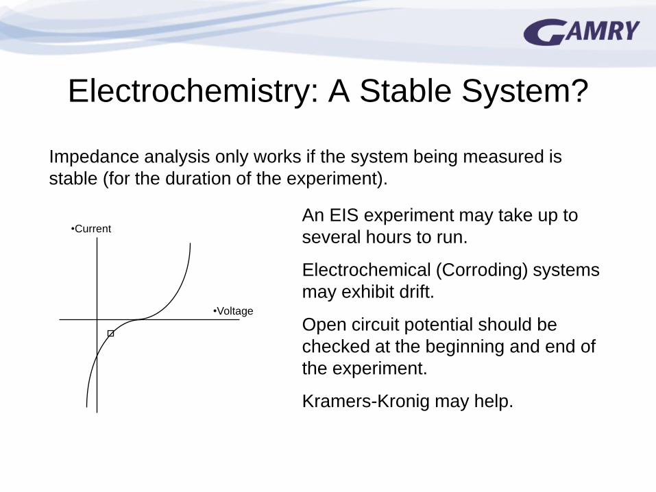
Electrochemistry: A Stable System?

Impedance analysis only works if the system being measured is

stable (for the duration of the experiment).

An EIS experiment may take up to

several hours to run.

Electrochemical (Corroding) systems

may exhibit drift.

Open circuit potential should be

checked at the beginning and end of

the experiment.

Kramers-Kronig may help.

•Current

•Voltage

Kramers-Kronig Transform

• The K-K Transform states that the phase and magnitude in a

real (linear, stable, and causal) system are related.

• Apply the Transform to the EIS data. Calculate the magnitude

from the experimental phase. If the calculated magnitudes

match the experimental magnitudes, then you can have some

confidence in the data. The converse is also true.

• If the values do not match, then the probability is high that your

system is not linear, not stable, or not causal.

• The K-K Transform as a validator of the data is not accepted by

all of the electrochemical community.

Bad K-K

Steps to Doing Analysis

• Look at data – Run K-K

– Determine number of RC loops

– Figure whether L or W exists • If W determine boundary conditions

• Pick/design a model

• Fit it – Check to see if CPEs/Transmission Lines needed

• Repeat as necessary

• Extract data

EIS Instrumentation

• Potentiostat/Galvanostat

• Sine wave generator

• Time synchronization (phase locking)

• All-in-ones, Portable & Floating Systems

Things to be aware of…

• Software – Control & Analysis

• Accuracy

• Performance limitations

EIS Take Home

• EIS is a versatile technique

– Non-destructive

– High information content

• Running EIS is easy

• EIS modeling analysis is very powerful

– Simplest working model is best

– Complex system analysis is possible

– User expertise can be helpful

References for EIS

• Electrochemical Impedance and Noise, R. Cottis and S.

Turgoose, NACE International, 1999. ISBN 1-57590-093-9.

An excellent tutorial that is highly recommended.

• Electrochemical Techniques in Corrosion Engineering, 1986,

NACE International

Proceedings from a Symposium held in 1986. 36 papers.

Covers the basics of the various electrochemical techniques and

a wide variety of papers on the application of these techniques.

Includes impedance spectroscopy.

• Electrochemical Impedance: Analysis and Interpretation, STP

1188, Edited by Scully, Silverman, and Kendig, ASTM, ISBN 0-

8031-1861-9.

26 papers covering modeling, corrosion, inhibitors, soil,

concrete, and coatings.

• EIS Primer, Gamry Instruments website, www.gamry.com

a practical beginner s guide to cyclic voltammetry · a practical beginner’s guide to cyclic...

Documents