A practical method for calculating largest Lyapunovexponents from small data sets

Michael T. Rosenstein, James J. Collins, and Carlo J. De Luca

NeuroMuscular Research Center and Department of Biomedical Engineering,

Boston University, 44 Cummington Street, Boston, MA 02215, USA

November 20, 1992

Running Title: Lyapunov exponents from small data sets

Key Words: chaos, Lyapunov exponents, time series analysis

PACS codes: 05.45.+b, 02.50.+s, 02.60.+y

Corresponding Author: Michael T. RosensteinNeuroMuscular Research CenterBoston University44 Cummington StreetBoston, MA 02215USA

Telephone: (617) 353-9757Fax: (617) 353-5737Internet: ROSENSTEIN@BUNMRG.BU.EDU

Abstract

Detecting the presence of chaos in a dynamical system is an important problem that is

solved by measuring the largest Lyapunov exponent. Lyapunov exponents quantify the

exponential divergence of initially close state-space trajectories and estimate the amount of chaos

in a system. We present a new method for calculating the largest Lyapunov exponent from an

experimental time series. The method follows directly from the definition of the largest

Lyapunov exponent and is accurate because it takes advantage of all the available data. We

show that the algorithm is fast, easy to implement, and robust to changes in the following

quantities: embedding dimension, size of data set, reconstruction delay, and noise level.

Furthermore, one may use the algorithm to calculate simultaneously the correlation dimension.

Thus, one sequence of computations will yield an estimate of both the level of chaos and the

system complexity.

1

1. Introduction Over the past decade, distinguishing deterministic chaos from noise has become an

important problem in many diverse fields, e.g., physiology [18], economics [11]. This is due, in

part, to the availability of numerical algorithms for quantifying chaos using experimental time

series. In particular, methods exist for calculating correlation dimension (D2 ) [20], Kolmogorov

entropy [21], and Lyapunov characteristic exponents [15, 17, 32, 39]. Dimension gives an

estimate of the system complexity; entropy and characteristic exponents give an estimate of the

level of chaos in the dynamical system.

The Grassberger-Procaccia algorithm (GPA) [20] appears to be the most popular method

used to quantify chaos. This is probably due to the simplicity of the algorithm [16] and the fact

that the same intermediate calculations are used to estimate both dimension and entropy.

However, the GPA is sensitive to variations in its parameters, e.g., number of data points [28],

embedding dimension [28], reconstruction delay [3], and it is usually unreliable except for long,

noise-free time series. Hence, the practical significance of the GPA is questionable, and the

Lyapunov exponents may provide a more useful characterization of chaotic systems.

For time series produced by dynamical systems, the presence of a positive characteristic

exponent indicates chaos. Furthermore, in many applications it is sufficient to calculate only the

largest Lyapunov exponent (λ1). However, the existing methods for estimating λ1 suffer from

at least one of the following drawbacks: (1) unreliable for small data sets, (2) computationally

intensive, (3) relatively difficult to implement. For this reason, we have developed a new

method for calculating the largest Lyapunov exponent. The method is reliable for small data

sets, fast, and easy to implement. “Easy to implement” is largely a subjective quality, although

we believe it has had a notable positive effect on the popularity of dimension estimates.

The remainder of this paper is organized as follows. Section 2 describes the Lyapunov

spectrum and its relation to Kolmogorov entropy. A synopsis of previous methods for

calculating Lyapunov exponents from both system equations and experimental time series is also

2

given. In Section 3 we describe the new approach for calculating λ1 and show how it differs

from previous methods. Section 4 presents the results of our algorithm for several chaotic

dynamical systems as well as several non-chaotic systems. We show that the method is robust to

variations in embedding dimension, number of data points, reconstruction delay, and noise level.

Section 5 is a discussion that includes a description of the procedure for calculating λ1 and D2

simultaneously. Finally, Section 6 contains a summary of our conclusions.

2. BackgroundFor a dynamical system, sensitivity to initial conditions is quantified by the Lyapunov

exponents. For example, consider two trajectories with nearby initial conditions on an attracting

manifold. When the attractor is chaotic, the trajectories diverge, on average, at an exponential

rate characterized by the largest Lyapunov exponent [15]. This concept is also generalized for

the spectrum of Lyapunov exponents, λ i (i=1, 2, ..., n), by considering a small n-dimensional

sphere of initial conditions, where n is the number of equations (or, equivalently, the number of

state variables) used to describe the system. As time (t) progresses, the sphere evolves into an

ellipsoid whose principal axes expand (or contract) at rates given by the Lyapunov exponents.

The presence of a positive exponent is sufficient for diagnosing chaos and represents local

instability in a particular direction. Note that for the existence of an attractor, the overall

dynamics must be dissipative, i.e., globally stable, and the total rate of contraction must

outweigh the total rate of expansion. Thus, even when there are several positive Lyapunov

exponents, the sum across the entire spectrum is negative.

Wolf et al. [39] explain the Lyapunov spectrum by providing the following geometrical

interpretation. First, arrange the n principal axes of the ellipsoid in the order of most rapidly

expanding to most rapidly contracting. It follows that the associated Lyapunov exponents will

be arranged such that

λ1 ≥ λ2 ≥ ... ≥ λn , (1)

3

where λ1 and λn correspond to the most rapidly expanding and contracting principal axes,

respectively. Next, recognize that the length of the first principal axis is proportional to eλ1t ; the

area determined by the first two principal axes is proportional to e(λ1 +λ2 )t ; and the volume

determined by the first k principal axes is proportional to e(λ1 +λ2 +...+λ k )t . Thus, the Lyapunov

spectrum can be defined such that the exponential growth of a k-volume element is given by the

sum of the k largest Lyapunov exponents. Note that information created by the system is

represented as a change in the volume defined by the expanding principal axes. The sum of the

corresponding exponents, i.e., the positive exponents, equals the Kolmogorov entropy (K) or

mean rate of information gain [15]:

K = λ iλ i >0∑ . (2)

When the equations describing the dynamical system are available, one can calculate the

entire Lyapunov spectrum [5, 34]. (See [39] for example computer code.) The approach

involves numerically solving the system’s n equations for n+1 nearby initial conditions. The

growth of a corresponding set of vectors is measured, and as the system evolves, the vectors are

repeatedly reorthonormalized using the Gram-Schmidt procedure. This guarantees that only one

vector has a component in the direction of most rapid expansion, i.e., the vectors maintain a

proper phase space orientation. In experimental settings, however, the equations of motion are

usually unknown and this approach is not applicable. Furthermore, experimental data often

consist of time series from a single observable, and one must employ a technique for attractor

reconstruction, e.g., method of delays [27, 37], singular value decomposition [8].

As suggested above, one cannot calculate the entire Lyapunov spectrum by choosing

arbitrary directions for measuring the separation of nearby initial conditions. One must measure

the separation along the Lyapunov directions which correspond to the principal axes of the

ellipsoid previously considered. These Lyapunov directions are dependent upon the system flow

and are defined using the Jacobian matrix, i.e., the tangent map, at each point of interest along

the flow [15]. Hence, one must preserve the proper phase space orientation by using a suitable

4

approximation of the tangent map. This requirement, however, becomes unnecessary when

calculating only the largest Lyapunov exponent.

If we assume that there exists an ergodic measure of the system, then the multiplicative

ergodic theorem of Oseledec [26] justifies the use of arbitrary phase space directions when

calculating the largest Lyapunov exponent with smooth dynamical systems. We can expect

(with probability 1) that two randomly chosen initial conditions will diverge exponentially at a

rate given by the largest Lyapunov exponent [6, 15]. In other words, we can expect that a

random vector of initial conditions will converge to the most unstable manifold, since

exponential growth in this direction quickly dominates growth (or contraction) along the other

Lyapunov directions. Thus, the largest Lyapunov exponent can be defined using the following

equation where d(t) is the average divergence at time t and C is a constant that normalizes the

initial separation:

d(t) = Ceλ1t . (3)

For experimental applications, a number of researchers have proposed algorithms that

estimate the largest Lyapunov exponent [1, 10, 12, 16, 17, 29, 33, 38-40], the positive Lyapunov

spectrum, i.e., only positive exponents [39], or the complete Lyapunov spectrum [7, 9, 13, 15,

32, 35, 41]. Each method can be considered as a variation of one of several earlier approaches

[15, 17, 32, 39] and as suffering from at least one of the following drawbacks: (1) unreliable for

small data sets, (2) computationally intensive, (3) relatively difficult to implement. These

drawbacks motivated our search for an improved method of estimating the largest Lyapunov

exponent.

3. Current ApproachThe first step of our approach involves reconstructing the attractor dynamics from a

single time series. We use the method of delays [27, 37] since one goal of our work is to develop

a fast and easily implemented algorithm. The reconstructed trajectory, X , can be expressed as a

matrix where each row is a phase-space vector. That is,

5

X = X1 X2 ... XM[ ]T , (4)

where Xi is the state of the system at discrete time i. For an N-point time series, x1, x2 ,..., xN{ },

each Xi is given by

Xi = xi xi+ J ... xi+(m−1)J[ ] , (5)

where J is the lag or reconstruction delay, and m is the embedding dimension. Thus, X is an

M × m matrix, and the constants m, M, J, and N are related as

M = N − (m − 1)J . (6)

The embedding dimension is usually estimated in accordance with Takens’ theorem, i.e.,

m > 2n, although our algorithm often works well when m is below the Takens criterion. A

method used to choose the lag via the correlation sum was addressed by Liebert and Schuster

[23] (based on [19]). Nevertheless, determining the proper lag is still an open problem [4]. We

have found a good approximation of J to equal the lag where the autocorrelation function drops

to 1 − 1e of its initial value. Calculating this J can be accomplished using the fast Fourier

transform (FFT), which requires far less computation than the approach of Liebert and Schuster.

Note that our algorithm also works well for a wide range of lags, as shown in Section 4.3.

After reconstructing the dynamics, the algorithm locates the nearest neighbor of each

point on the trajectory. The nearest neighbor, Xj, is found by searching for the point that

minimizes the distance to the particular reference point, X j . This is expressed as

d j (0) = minX

j

X j − Xj

, (7)

where d j (0) is the initial distance from the j th point to its nearest neighbor, and .. denotes the

Euclidean norm. We impose the additional constraint that nearest neighbors have a temporal

separation greater than the mean period of the time series:1

1 We estimated the mean period as the reciprocal of the mean frequency of the power spectrum,

although we expect any comparable estimate, e.g., using the median frequency of the magnitude

spectrum, to yield equivalent results.

6

j − j > mean period . (8)

This allows us to consider each pair of neighbors as nearby initial conditions for different

trajectories. The largest Lyapunov exponent is then estimated as the mean rate of separation of

the nearest neighbors.

To this point, our approach for calculating λ1 is similar to previous methods that track

the exponential divergence of nearest neighbors. However, it is important to note some

differences:

1) The algorithm by Wolf et al. [39] fails to take advantage of all the available data because it

focuses on one “fiducial” trajectory. A single nearest neighbor is followed and repeatedly

replaced when its separation from the reference trajectory grows beyond a certain limit.

Additional computation is also required because the method approximates the Gram-Schmidt

procedure by replacing a neighbor with one that preserves its phase space orientation.

However, as shown in Section 2, this preservation of phase space orientation is unnecessary

when calculating only the largest Lyapunov exponent.

2) If a nearest neighbor precedes (temporally) its reference point, then our algorithm can be

viewed as a “prediction” approach. (In such instances, the predictive model is a simple delay

line, the prediction is the location of the nearest neighbor, and the prediction error equals the

separation between the nearest neighbor and its reference point.) However, other prediction

methods use more elaborate schemes, e.g., polynomial mappings, adaptive filters, neural

networks, that require much more computation. The amount of computation for the Wales

method [38] (based on [36]) is also greater, although it is comparable to the present

approach. We have found the Wales algorithm to give excellent results for discrete systems

derived from difference equations, e.g., logistic, Hénon, but poor results for continuous

systems derived from differential equations, e.g., Lorenz, Rössler.

3) The current approach is principally based on the work of Sato et al. [33] which estimates λ1

as

7

λ1(i) = 1i ⋅ ∆t

⋅ 1(M − i)

lnd j (i)

d j (0)j=1

M−i

∑ , (9)

where ∆t is the sampling period of the time series, and d j (i) is the distance between the j th

pair of nearest neighbors after i discrete-time steps, i.e., i ⋅ ∆t seconds. (Recall that M is the

number of reconstructed points as given in Eq. (6).) In order to improve convergence (with

respect to i), Sato et al. [33] give an alternate form of Eq. (9):

λ1(i,k) = 1k ⋅ ∆t

⋅ 1(M − k)

lnd j (i + k)

d j (i)j=1

M−k

∑ . (10)

In Eq. (10), k is held constant, and λ1 is extracted by locating the plateau of λ1(i,k) with

respect to i. We have found that locating this plateau is sometimes problematic, and the

resulting estimates of λ1 are unreliable. As discussed in Section 5.3, this difficulty is due to

the normalization by d j (i) .

The remainder of our method proceeds as follows. From the definition of λ1 given in

Eq. (3), we assume the j th pair of nearest neighbors diverge approximately at a rate given by the

largest Lyapunov exponent:

d j (i) ≈ Cjeλ1(i⋅∆t) , (11)

where Cj is the initial separation. By taking the logarithm of both sides of Eq. (11), we obtain

ln d j (i) ≈ lnCj + λ1(i ⋅ ∆t) . (12)

Eq. (12) represents a set of approximately parallel lines (for j = 1,2,..., M ), each with a slope

roughly proportional to λ1. The largest Lyapunov exponent is easily and accurately calculated

using a least-squares fit to the “average” line defined by

y(i) = 1∆t ln d j (i) , (13)

where .. denotes the average over all values of j. This process of averaging is the key to

calculating accurate values of λ1 using small, noisy data sets. Note that in Eq. (11), Cj performs

the function of normalizing the separation of the neighbors, but as shown in Eq. (12), this

8

normalization is unnecessary for estimating λ1. By avoiding the normalization, the current

approach gains a slight computational advantage over the method by Sato et al.

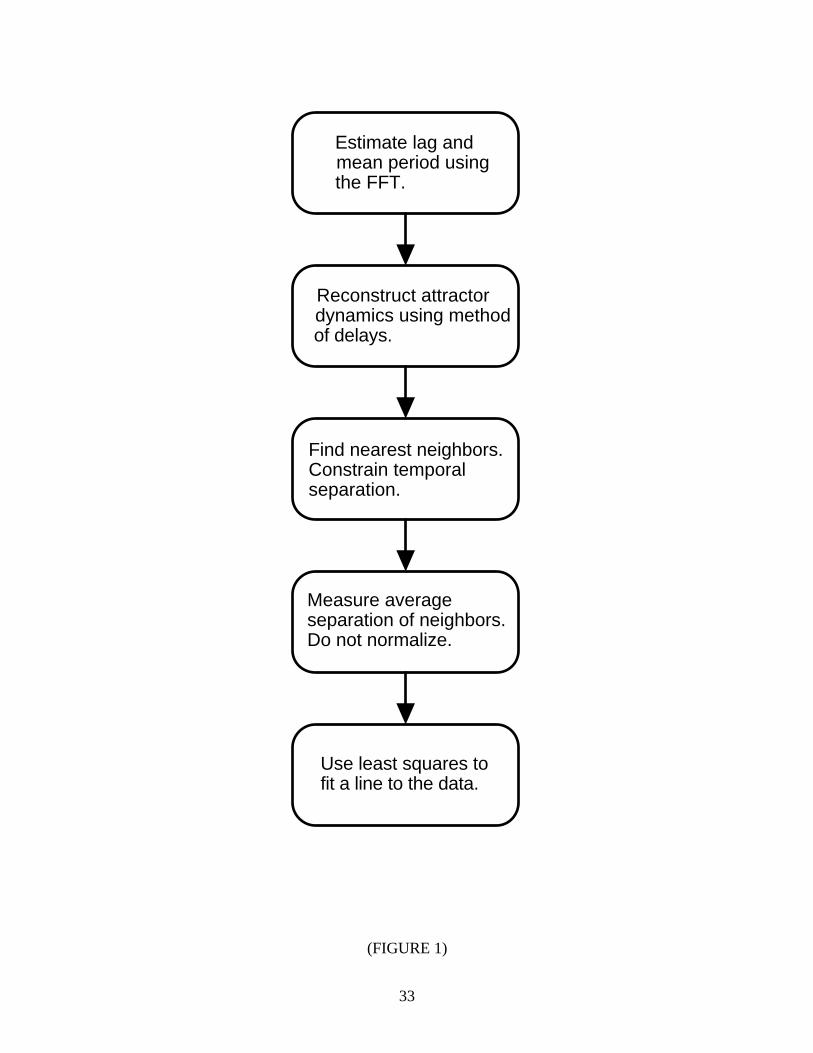
*** FIGURE 1 NEAR HERE ***

The new algorithm for calculating largest Lyapunov exponents is outlined in Figure 1.

This method is easy to implement and fast because it uses a simple measure of exponential

divergence that circumvents the need to approximate the tangent map. The algorithm is also

attractive from a practical standpoint because it does not require large data sets and it

simultaneously yields the correlation dimension (discussed in Section 5.5). Furthermore, the

method is accurate for small data sets because it takes advantage of all the available data. In the

next section, we present the results for several dynamical systems.

4. Experimental ResultsTable I summarizes the chaotic systems primarily examined in this paper. The

differential equations were solved numerically using a fourth-order Runge-Kutta integration with

a step size equal to ∆t as given in Table I. For each system, the initial point was chosen near the

attractor and the transient points were discarded. In all cases, the x-coordinate time series was

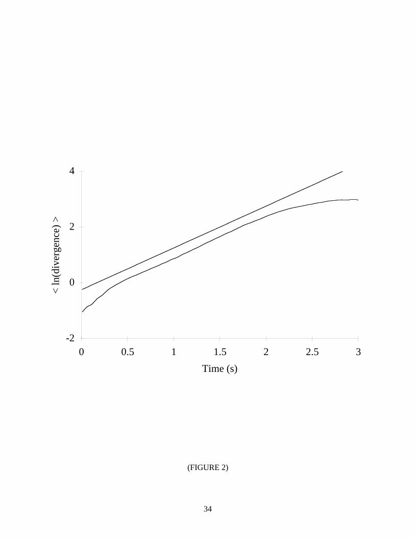
used to reconstruct the dynamics. Figure 2 shows a typical plot (solid curve) of ln d j (i) versus

i ⋅ ∆t ;2 the dashed line has a slope equal to the theoretical value of λ1. After a short transition,

there is a long linear region that is used to extract the largest Lyapunov exponent. The curve

saturates at longer times since the system is bounded in phase space and the average divergence

cannot exceed the “length” of the attractor.

*** TABLE I & FIGURE 2 NEAR HERE ***

The remainder of this section contains tabulated results from our algorithm under

different conditions. The corresponding plots are meant to give the reader qualitative

information about the facility of extracting λ1 from the data. That is, the more prominent the

2 In each figure, “< ln(divergence) >” and “Time (s)” are used to denote ln d j (i) and i ⋅ ∆t ,

respectively.

9

linear region, the easier one can extract the correct slope. (Repeatability is discussed in Section

5.2.)

4.1. Embedding dimension

Since we normally have no a priori knowledge concerning the dimension of a system, it

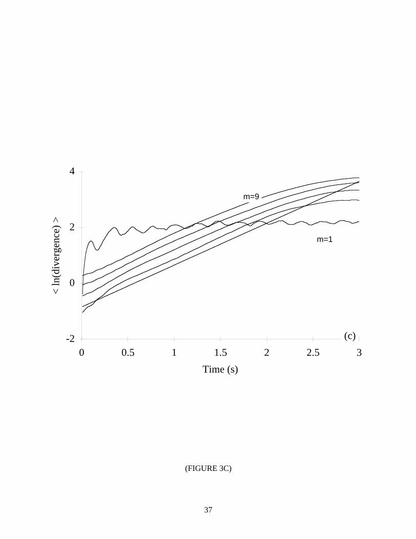
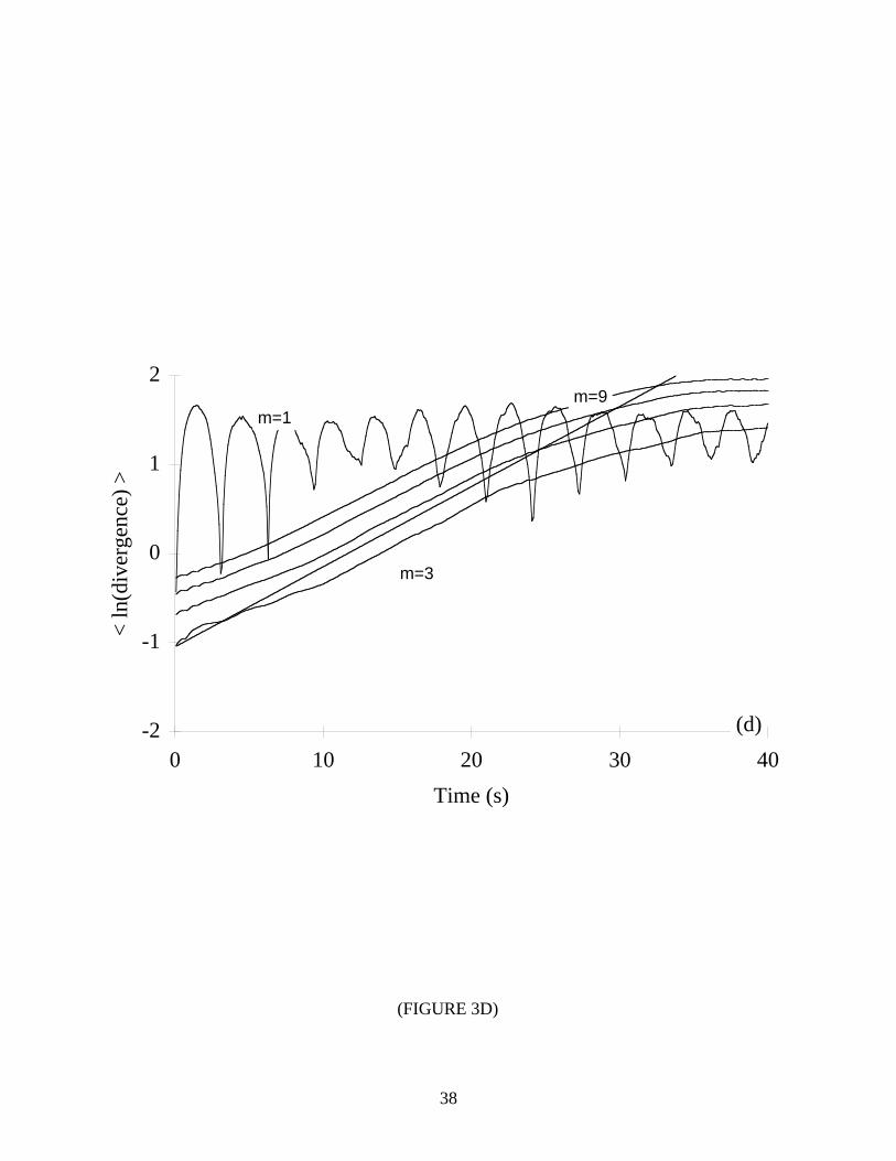
is imperative that we evaluate our method for different embedding dimensions. Table II and

Figure 3 show our findings for several values of m. In all but three cases (m=1 for the Hénon,

Lorenz, and Rössler systems), the error was less than ±10%, and most errors were less than ±5%.

It is apparent that satisfactory results are obtained only when m is at least equal to the topological

dimension of the system, i.e., m ≥ n . This is due to the fact that chaotic systems are effectively

stochastic when embedded in a phase space that is too small to accommodate the true dynamics.

Notice that the algorithm performs quite well when m is below the Takens criterion. Therefore,

it seems one may choose the smallest embedding dimension that yields a convergence of the

results.

*** TABLE II & FIGURE 3 NEAR HERE ***

4.2. Length of time series

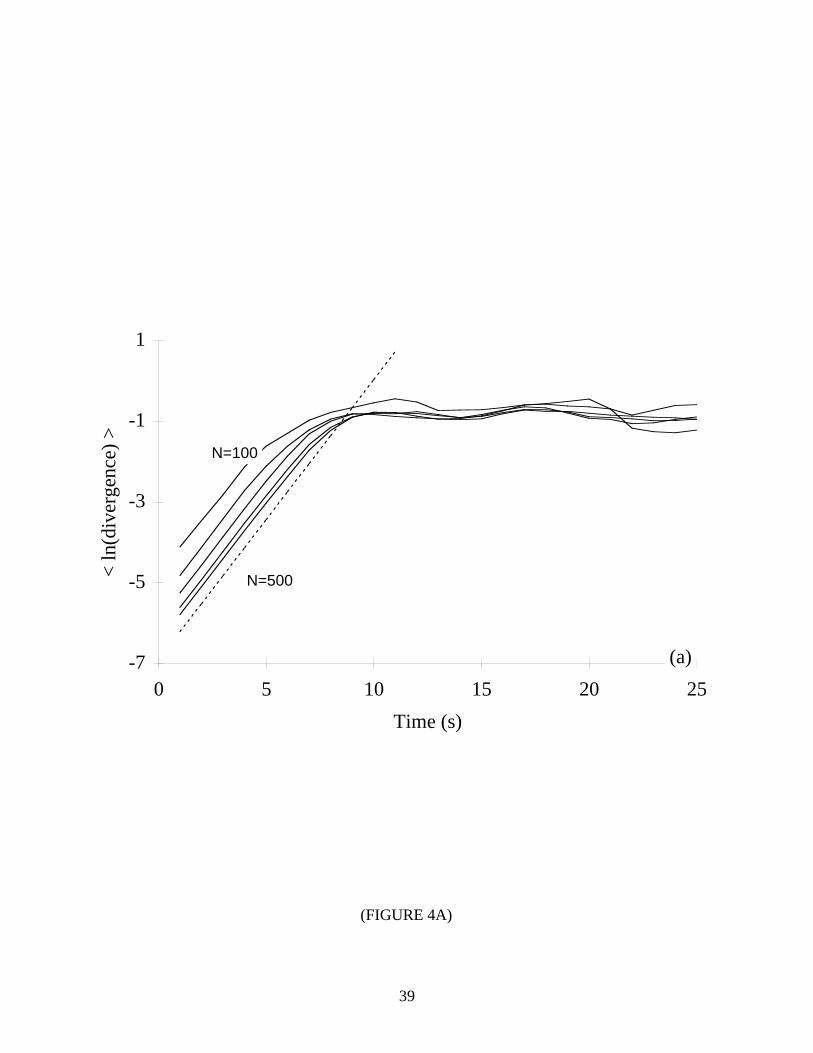
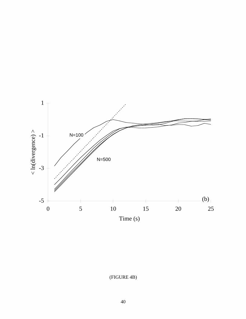
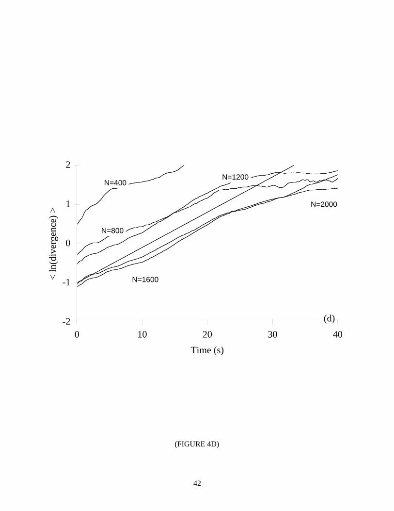
Next we consider the performance of our algorithm for time series of various lengths. As

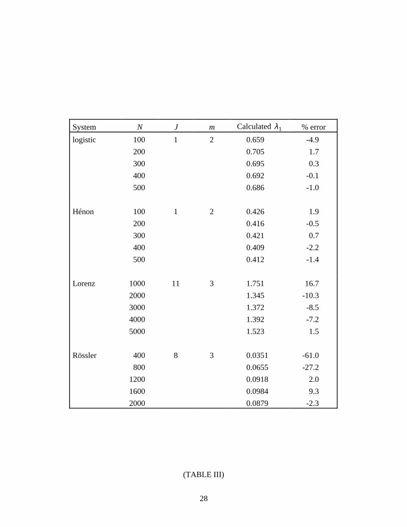
shown in Table III and Figure 4, the present method also works well when N is small (N=100 to

1000 for the examined systems). Again, the error was less than ±10% in almost all cases. (The

greatest difficulty occurs with the Rössler attractor. For this system, we also found a 20-25%

negative bias in the results for N=3000 to 5000.) To our knowledge, the lower limit of N used in

each case is less than the smallest value reported in the literature. (The only exception is due to

Briggs [7], who examined the Lorenz system with N=600. However, Briggs reported errors for

λ1 that ranged from 54% to 132% for this particular time series length.) We also point out that

the literature [1, 9, 13, 15, 35] contains results for values of N that are an order of magnitude

greater than the largest values used here.

*** TABLE III & FIGURE 4 NEAR HERE ***

10

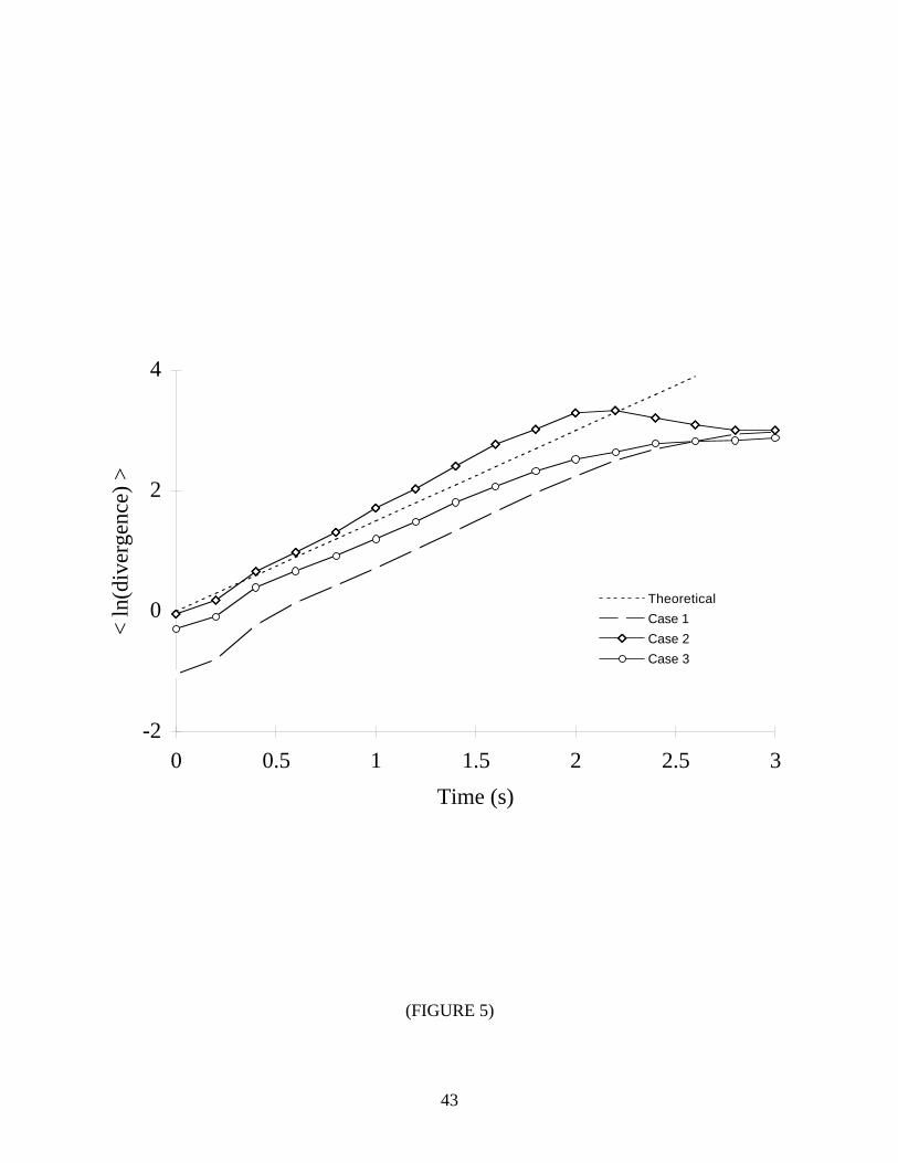
It is important to mention that quantitative analyses of chaotic systems are usually

sensitive to not only the data size (in samples), but also the observation time (in seconds).

Hence, we examined the interdependence of N and N ⋅ ∆t for the Lorenz system. Figure 5 shows

the output of our algorithm for three different sampling conditions: (1) N = 5000 , ∆t = 0.01 s

( N ⋅ ∆t = 50 s); (2) N = 1000 , ∆t = 0.01 s (N ⋅ ∆t = 10 s); and (3) N = 1000 , ∆t = 0.05 s

( N ⋅ ∆t = 50 s). The latter two time series were derived from the former by using the first 1000

points and every fifth point, respectively. As expected, the best results were obtained with a

relatively long observation time and closely-spaced samples (Case 1). However, we saw

comparable results with the long observation time and widely-spaced samples (Case 3). As long

as ∆t is small enough to ensure a minimum number of points per orbit of the attractor

(approximately n to 10n points [39]), it is better to decrease N by reducing the sampling rate and

not the observation time.

*** FIGURE 5 NEAR HERE ***

4.3. Reconstruction delay

As commented in Section 3, determining the proper reconstruction delay is still an open

problem. For this reason, it is necessary to test our algorithm with different values of J. (See

Table IV and Figure 6.) Since discrete maps are most faithfully reconstructed with a delay equal

to one, it is not surprising that the best results were seen with the lag equal to one for the logistic

and Hénon systems (errors of -1.7% and -2.2%, respectively). For the Lorenz and Rössler

systems, the algorithm performed well (error ≤ 7%) with all lags except the extreme ones (J=1,

41 for Lorenz; J=2, 26 for Rössler). Thus, we expect satisfactory results whenever the lag is

determined using any common method such as those based on the autocorrelation function or the

correlation sum. Notice that the smallest errors were obtained for the lag where the

autocorrelation function drops to 1 − 1e of its initial value.

*** TABLE IV & FIGURE 6 NEAR HERE ***

11

4.4. Additive noise

Next, we consider the effects of additive noise, i.e., measurement or instrumentation

noise. This was accomplished by examining several time series produced by a superposition of

white noise and noise-free data (noise-free up to the computer precision). Before superposition,

the white noise was scaled by an appropriate factor in order to achieve a desired signal-to-noise

ratio (SNR). The SNR is the ratio of the power (or, equivalently, the variance) in the noise-free

signal and that of the pure-noise signal. A signal-to-noise ratio greater than about 1000 can be

regarded as low noise and a SNR less than about 10 as high noise.

The results are shown in Table V and Figure 7. We expect satisfactory estimates of λ1

except in extremely noisy situations. With low noise, the error was smaller than ±10% in each

case. At moderate noise levels (SNR ranging from about 100 to 1000), the algorithm performed

reasonably well with an error that was generally near ±25%. As expected, the poorest results

were seen with the highest noise levels (SNR less than or equal to 10). (We believe that the

improved performance with the logistic map and low signal-to-noise ratios is merely

coincidental. The reader should equate the shortest linear regions in Figure 7 with the highest

noise and greatest uncertainty in estimating λ1.) It seems one cannot expect to estimate the

largest Lyapunov exponent in high-noise environments; however, the clear presence of a positive

slope still affords one the qualitative confirmation of a positive exponent (and chaos).

*** TABLE V & FIGURE 7 NEAR HERE ***

It is important to mention that the adopted noise model represents a “worst-case” scenario

because white noise contaminates a signal across an infinite bandwidth. (Furthermore, we

consider signal-to-noise ratios that are substantially lower than most values previously reported

in the literature.) Fortunately, some of the difficulties are remedied by filtering, which is

expected to preserve the exponential divergence of nearest neighbors [39]. Whenever we

remove noise while leaving the signal intact, we can expect an improvement in system

predictability and, hence, in our ability to detect chaos. In practice, however, caution is

12

warranted because the underlying signal may have some frequency content in the stopband or the

filter may substantially alter the phase in the passband.

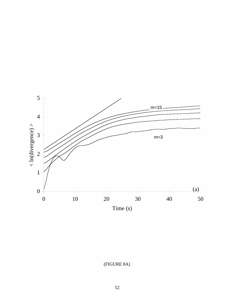
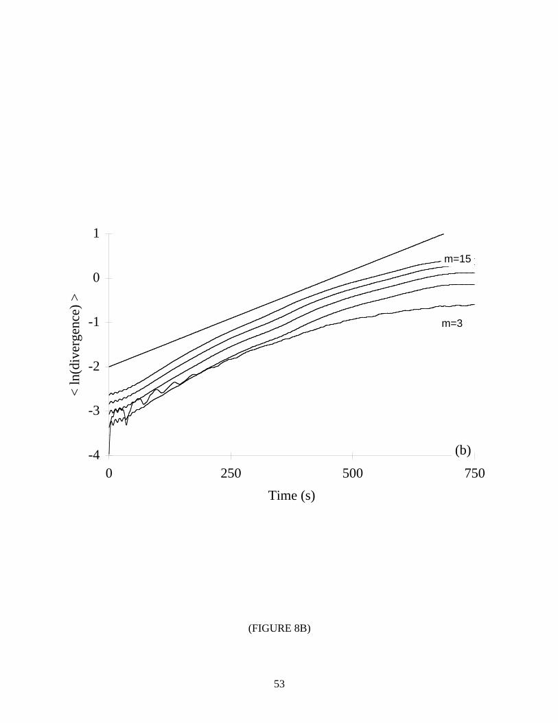
4.5. Two positive Lyapunov exponents

As described in Section 2, it is unnecessary to preserve phase space orientation when

calculating the largest Lyapunov exponent. In order to provide experimental verification of this

theory, we consider the performance of our algorithm with two systems that possess more than

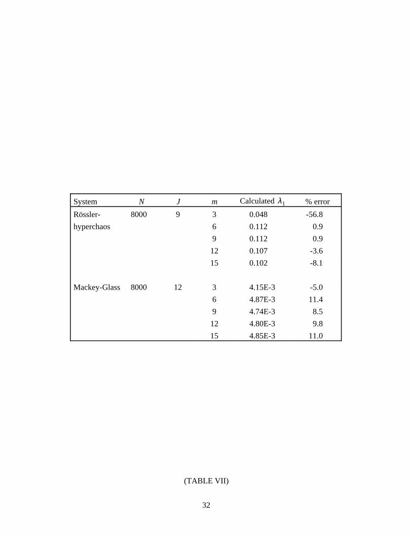
one positive exponent: Rössler-hyperchaos [30] and Mackey-Glass [25]. (See Table VI for

details.) The results are shown in Table VII and Figure 8. For both systems, the errors were

typically less than ±10%. From these results, we conclude that the algorithm measures

exponential divergence along the most unstable manifold and not along some other Lyapunov

direction. However, notice the predominance of a negative bias in the errors presented in

Sections 4.1-4.4. We believe that over short time scales, some nearest neighbors explore

Lyapunov directions other than that of the largest Lyapunov exponent. Thus, a small

underestimation (less than 5%) of λ1 is expected.

*** TABLE VI NEAR HERE ***

*** TABLE VII & FIGURE 8 NEAR HERE ***

4.6. Non-chaotic systems

As stated earlier, distinguishing deterministic chaos from noise has become an important

problem. It follows that effective algorithms for detecting chaos must accurately characterize

both chaotic and non-chaotic systems; a reliable algorithm is not “fooled” by difficult systems

such as correlated noise. Hence, we further establish the utility of our method by examining its

performance with the following non-chaotic systems: two-torus, white noise, bandlimited noise,

and “scrambled” Lorenz.

For each system, a 2000-point time series was generated. The two-torus is an example of

a quasiperiodic, deterministic system. The corresponding time series, x(i), was created by a

superposition of two sinusoids with incommensurate frequencies:

13

x(i) = sin(2πf1 ⋅ i ⋅ ∆t) + sin(2πf 2 ⋅ i ⋅ ∆t) , (14)

where f1 = 1.732051 ≈ 3 Hz, f 2 = 2.236068 ≈ 5 Hz, and the sampling period was

∆t = 0.01 s. White noise and bandlimited noise are stochastic systems that are analogous to

discrete and continuous chaotic systems, respectively. The “scrambled” Lorenz also represents a

continuous stochastic system, and the data set was generated by randomizing the phase

information from the Lorenz attractor. This procedure yields a time series of correlated noise

with spectral characteristics identical to that of the Lorenz attractor.

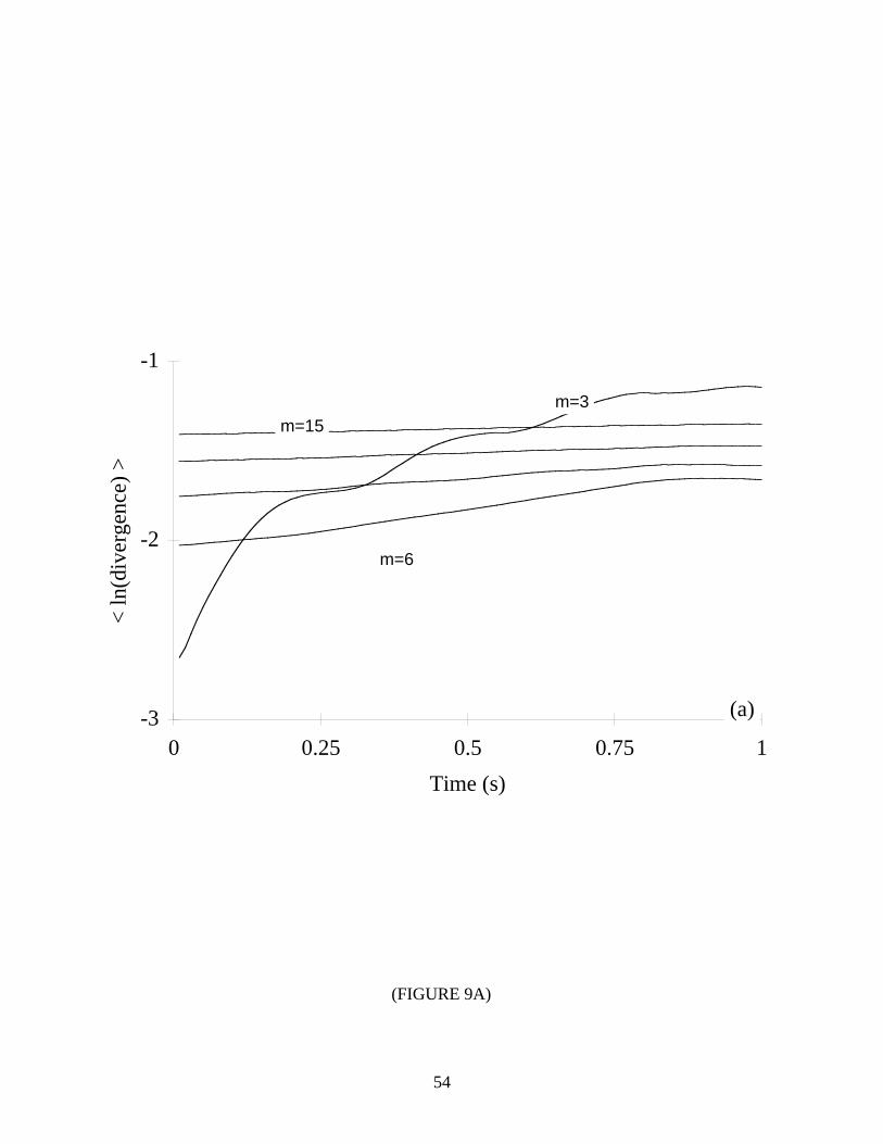
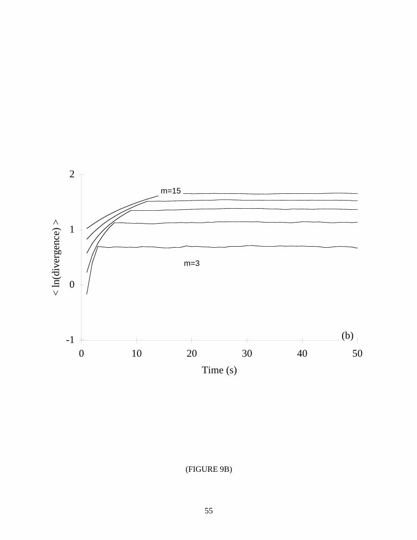
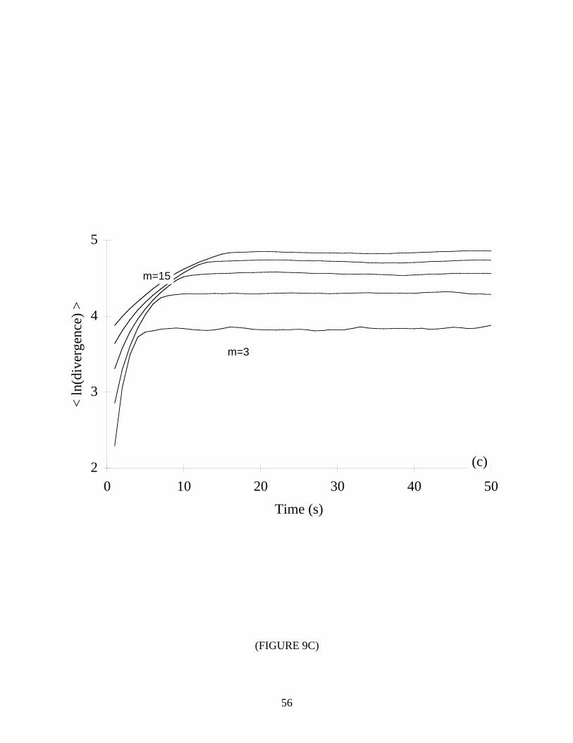
For quasiperiodic and stochastic systems we expect flat plots of ln d j (i) versus i ⋅ ∆t .

That is, on average the nearest neighbors should neither diverge nor converge. Additionally,

with the stochastic systems we expect an initial “jump” from a small separation at t=0. The

results are shown in Figure 9, and as expected, the curves are mostly flat. However, notice the

regions that could be mistaken as appropriate for extracting a positive Lyapunov exponent.

Fortunately, our empirical results suggest that one may still detect non-chaotic systems for the

following reasons:

1) The anomalous scaling region is not linear since the divergence of nearest neighbors is not

exponential.

2) For stochastic systems, the anomalous scaling region flattens with increasing embedding

dimension. Finite dimensional systems exhibit a convergence once the embedding

dimension is large enough to accomodate the dynamics, whereas stochastic systems fail to

show a convergence because they appear more ordered in higher embedding spaces. With

the two-torus, we attribute the lack of convergence to the finite precision “noise” in the data

set. (Notice the small average divergence even at i ⋅ ∆t=1.) Strictly speaking, we can only

distinguish high-dimensional systems from low-dimensional ones, although in most

applications a high-dimensional system may be considered random, i.e., infinite-dimensional.

*** FIGURE 9 NEAR HERE ***

14

5. Discussion

5.1. Eckmann-Ruelle requirement

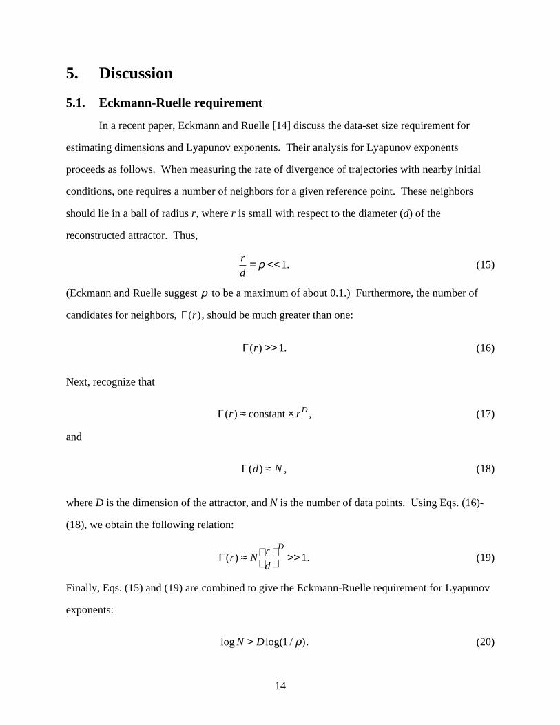
In a recent paper, Eckmann and Ruelle [14] discuss the data-set size requirement for

estimating dimensions and Lyapunov exponents. Their analysis for Lyapunov exponents

proceeds as follows. When measuring the rate of divergence of trajectories with nearby initial

conditions, one requires a number of neighbors for a given reference point. These neighbors

should lie in a ball of radius r, where r is small with respect to the diameter (d) of the

reconstructed attractor. Thus,

r

d= ρ << 1. (15)

(Eckmann and Ruelle suggest ρ to be a maximum of about 0.1.) Furthermore, the number of

candidates for neighbors, Γ(r), should be much greater than one:

Γ(r) >> 1. (16)

Next, recognize that

Γ(r) ≈ constant × rD , (17)

and

Γ(d) ≈ N , (18)

where D is the dimension of the attractor, and N is the number of data points. Using Eqs. (16)-

(18), we obtain the following relation:

Γ(r) ≈ Nr

d

D

>> 1. (19)

Finally, Eqs. (15) and (19) are combined to give the Eckmann-Ruelle requirement for Lyapunov

exponents:

log N > D log(1 / ρ). (20)

15

For ρ = 0.1, Eq. (20) directs us to choose N such that

N > 10D . (21)

This requirement was met with all time series considered in this paper. Notice that any rigorous

definition of “small data set” should be a function of dimension. However, for comparative

purposes we regard a small data set as one that is small with respect to those previously

considered in the literature.

5.2. Repeatability

When using the current approach for estimating largest Lyapunov exponents, one is faced

with the following issue of repeatability: Can one consistently locate the region for extracting

λ1 without a guide, i.e., without a priori knowledge of the correct slope in the linear region?3

To address this issue, we consider the performance of our algorithm with multiple realizations of

the Lorenz attractor.

Three 5000-point time series from the Lorenz attractor were generated by partitioning one

15000-point data set into disjoint time series. Figure 10 shows the results using a visual format

similar to that first used by Abraham et al. [2] for estimating dimensions. Each curve is a plot of

slope versus time, where the slope is calculated from a least-squares fit to 51-point segments of

the ln d j (i) versus i ⋅ ∆t curve. We observe a clear and repeatable plateau from about

i ⋅ ∆t=0.6 to about i ⋅ ∆t=1.6. By using this range to define the region for extracting λ1, we

obtain a reliable estimate of the largest Lyapunov exponent: λ1=1.57 ± 0.03. (Recall that the

theoretical value is 1.50.)

*** FIGURE 10 NEAR HERE ***

3 In Tables II-IV, there appear to be inconsistent results when using identical values of N, J, and

m for a particular system. These small discrepencies are due to the subjective nature in choosing

the linear region and not the algorithm itself. In fact, the same output file was used to compute

λ1 in each case.

16

5.3. Relation to the Sato algorithm

As stated in Section 3, the current algorithm is principally based on the work of Sato et

al. [33]. More specifically, our approach can be considered as a generalization of the Sato

algorithm. To show this, we first rewrite Eq. (10) using .. to denote the average over all values

of j:

λ1(i,k) = 1k ⋅ ∆t

lnd j (i + k)

d j (i) . (22)

This equation is then rearranged and expressed in terms of the output from the current algorithm,

y(i) (from Eq. (13)):

λ1(i,k) = 1k ⋅ ∆t

ln d j (i + k) − ln d j (i)[ ]≈ 1

ky(i + k) − y(i)[ ]

.

(23)

Eq. (23) is interpreted as a finite-differences numerical differentiation of y(i) , where k specifies

the size of the differentiation interval.

Next, we attempt to derive y(i) from the output of the Sato algorithm by summing

λ1(i,k). That is, we define ′y ( ′i ) as

′y ( ′i ) = λ1(i,k) =i=0

′i

∑ 1k

y(i + k)i=0

′i

∑ − y(i)i=0

′i

∑

. (24)

By manipulating this equation, we can show that Eq. (23) is not invertible:

′y ( ′i ) = 1k

y(i)i=0

′i +k

∑ − y(i)i=0

k−1

∑ − y(i)i=0

′i

∑

= 1k

y(i)i= ′i +1

′i +k

∑ − y(i)i=0

k−1

∑

= 1k

y(i)i= ′i +1

′i +k

∑ + constant

.

(25)

If we disregard the constant in Eq. (25), ′y ( ′i ) is equivalent to y(i) smoothed by a k-point

moving-average filter.

17

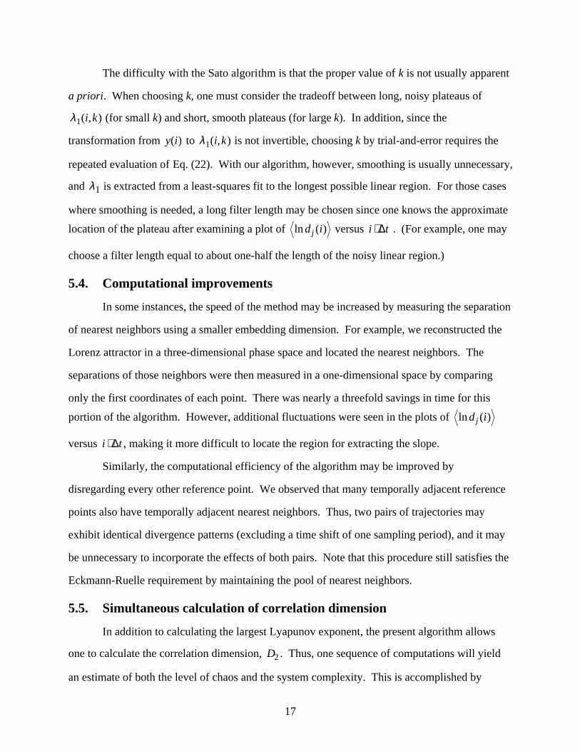
The difficulty with the Sato algorithm is that the proper value of k is not usually apparent

a priori. When choosing k, one must consider the tradeoff between long, noisy plateaus of

λ1(i,k) (for small k) and short, smooth plateaus (for large k). In addition, since the

transformation from y(i) to λ1(i,k) is not invertible, choosing k by trial-and-error requires the

repeated evaluation of Eq. (22). With our algorithm, however, smoothing is usually unnecessary,

and λ1 is extracted from a least-squares fit to the longest possible linear region. For those cases

where smoothing is needed, a long filter length may be chosen since one knows the approximate

location of the plateau after examining a plot of ln d j (i) versus i ⋅ ∆t . (For example, one may

choose a filter length equal to about one-half the length of the noisy linear region.)

5.4. Computational improvements

In some instances, the speed of the method may be increased by measuring the separation

of nearest neighbors using a smaller embedding dimension. For example, we reconstructed the

Lorenz attractor in a three-dimensional phase space and located the nearest neighbors. The

separations of those neighbors were then measured in a one-dimensional space by comparing

only the first coordinates of each point. There was nearly a threefold savings in time for this

portion of the algorithm. However, additional fluctuations were seen in the plots of ln d j (i)

versus i ⋅ ∆t , making it more difficult to locate the region for extracting the slope.

Similarly, the computational efficiency of the algorithm may be improved by

disregarding every other reference point. We observed that many temporally adjacent reference

points also have temporally adjacent nearest neighbors. Thus, two pairs of trajectories may

exhibit identical divergence patterns (excluding a time shift of one sampling period), and it may

be unnecessary to incorporate the effects of both pairs. Note that this procedure still satisfies the

Eckmann-Ruelle requirement by maintaining the pool of nearest neighbors.

5.5. Simultaneous calculation of correlation dimension

In addition to calculating the largest Lyapunov exponent, the present algorithm allows

one to calculate the correlation dimension, D2 . Thus, one sequence of computations will yield

an estimate of both the level of chaos and the system complexity. This is accomplished by

18

taking advantage of the numerous distance calculations performed during the nearest-neighbors

search.

The Grassberger-Procaccia algorithm [20] estimates dimension by examining the scaling

properties of the correlation sum, Cm (r) . For a given embedding dimension, m, Cm (r) is

defined as

Cm (r) = 2M(M − 1)

θ r − Xi − Xk[ ]i≠k∑ , (26)

where θ ..[ ] is the Heavyside function. Therefore, Cm (r) is interpreted as the fraction of pairs of

points that are separated by a distance less than or equal to r. Notice that the previous equation

and Eq. (7) of our algorithm require the same distance computations (disregarding the constraint

in Eq. (8)). By exploiting this redundancy, we obtain a more complete characterization of the

system using a negligible amount of additional computation.

6. SummaryWe have presented a new method for calculating the largest Lyapunov exponent from

experimental time series. The method follows directly from the definition of the largest

Lyapunov exponent and is accurate because it takes advantage of all the available data. The

algorithm is fast because it uses a simple measure of exponential divergence and works well with

small data sets. In addition, the current approach is easy to implement and robust to changes in

the following quantities: embedding dimension, size of data set, reconstruction delay, and noise

level. Furthermore, one may use the algorithm to calculate simultaneously the correlation

dimension.

Acknowledgments

This work was supported by the Rehabilitation Research and Development Service of

Veterans Affairs.

19

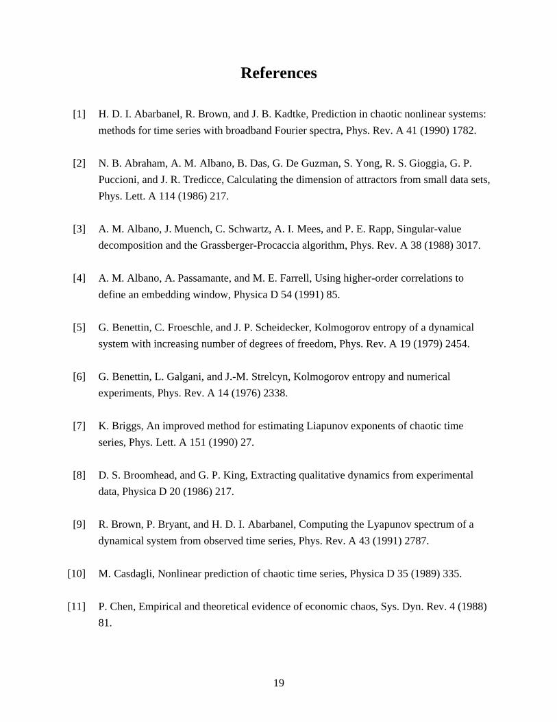
References

[1] H. D. I. Abarbanel, R. Brown, and J. B. Kadtke, Prediction in chaotic nonlinear systems:

methods for time series with broadband Fourier spectra, Phys. Rev. A 41 (1990) 1782.

[2] N. B. Abraham, A. M. Albano, B. Das, G. De Guzman, S. Yong, R. S. Gioggia, G. P.

Puccioni, and J. R. Tredicce, Calculating the dimension of attractors from small data sets,

Phys. Lett. A 114 (1986) 217.

[3] A. M. Albano, J. Muench, C. Schwartz, A. I. Mees, and P. E. Rapp, Singular-value

decomposition and the Grassberger-Procaccia algorithm, Phys. Rev. A 38 (1988) 3017.

[4] A. M. Albano, A. Passamante, and M. E. Farrell, Using higher-order correlations to

define an embedding window, Physica D 54 (1991) 85.

[5] G. Benettin, C. Froeschle, and J. P. Scheidecker, Kolmogorov entropy of a dynamical

system with increasing number of degrees of freedom, Phys. Rev. A 19 (1979) 2454.

[6] G. Benettin, L. Galgani, and J.-M. Strelcyn, Kolmogorov entropy and numerical

experiments, Phys. Rev. A 14 (1976) 2338.

[7] K. Briggs, An improved method for estimating Liapunov exponents of chaotic time

series, Phys. Lett. A 151 (1990) 27.

[8] D. S. Broomhead, and G. P. King, Extracting qualitative dynamics from experimental

data, Physica D 20 (1986) 217.

[9] R. Brown, P. Bryant, and H. D. I. Abarbanel, Computing the Lyapunov spectrum of a

dynamical system from observed time series, Phys. Rev. A 43 (1991) 2787.

[10] M. Casdagli, Nonlinear prediction of chaotic time series, Physica D 35 (1989) 335.

[11] P. Chen, Empirical and theoretical evidence of economic chaos, Sys. Dyn. Rev. 4 (1988)

81.

20

[12] J. Deppisch, H.-U. Bauer, and T. Geisel, Hierarchical training of neural networks and

prediction of chaotic time series, Phys. Lett. A 158 (1991) 57.

[13] J.-P. Eckmann, S. O. Kamphorst, D. Ruelle, and S. Ciliberto, Liapunov exponents from

time series, Phys. Rev. A 34 (1986) 4971.

[14] J.-P. Eckmann, and D. Ruelle, Fundamental limitations for estimating dimensions and

Lyapunov exponents in dynamical systems, Physica D 56 (1992) 185.

[15] J.-P. Eckmann, and D. Ruelle, Ergodic theory of chaos and strange attractors, Rev. Mod.

Phys. 57 (1985) 617.

[16] S. Ellner, A. R. Gallant, D. McCaffrey, and D. Nychka, Convergence rates and data

requirements for Jacobian-based estimates of Lyapunov exponents from data, Phys. Lett.

A 153 (1991) 357.

[17] J. D. Farmer, and J. J. Sidorowich, Predicting chaotic time series, Phys. Rev. Lett. 59

(1987) 845.

[18] G. W. Frank, T. Lookman, M. A. H. Nerenberg, C. Essex, J. Lemieux, and W. Blume,

Chaotic time series analysis of epileptic seizures, Physica D 46 (1990) 427.

[19] A. M. Fraser, and H. L. Swinney, Independent coordinates for strange attractors from

mutual information, Phys. Rev. A 33 (1986) 1134.

[20] P. Grassberger, and I. Procaccia, Characterization of strange attractors, Phys. Rev. Lett.

50 (1983) 346.

[21] P. Grassberger, and I. Procaccia, Estimation of the Kolmogorov entropy from a chaotic

signal, Phys. Rev. A 28 (1983) 2591.

[22] M. Hénon, A two-dimensional mapping with a strange attractor, Comm. Math. Phys. 50

(1976) 69.

[23] W. Liebert, and H. G. Schuster, Proper choice of the time delay for the analysis of chaotic

time series, Phys. Lett. A 142 (1989) 107.

21

[24] E. N. Lorenz, Deterministic nonperiodic flow, J. Atmos. Sci. 20 (1963) 130.

[25] M. C. Mackey, and L. Glass, Oscillation and chaos in physiological control systems,

Science 197 (1977) 287.

[26] V. I. Oseledec, A multiplicative ergodic theorem. Lyapunov characteristic numbers for

dynamical systems, Trans. Moscow Math. Soc. 19 (1968) 197.

[27] N. H. Packard, J. P. Crutchfield, J. D. Farmer, and R. S. Shaw, Geometry from a time

series, Phys. Rev. Lett. 45 (1980) 712.

[28] J. B. Ramsey, and H.-J. Yuan, The statistical properties of dimension calculations using

small data sets, Nonlinearity 3 (1990) 155.

[29]F. Rauf, and H. M. Ahmed, Calculation of Lyapunov exponents through nonlinear adaptive

filters, Proceedings IEEE International Symposium on Circuits and Systems, Singapore

(1991).

[30] O. E. Rössler, An equation for hyperchaos, Phys. Lett. A 71 (1979) 155.

[31] O. E. Rössler, An equation for continuous chaos, Phys. Lett. A 57 (1976) 397.

[32] M. Sano, and Y. Sawada, Measurement of the Lyapunov spectrum from a chaotic time

series, Phys. Rev. Lett. 55 (1985) 1082.

[33] S. Sato, M. Sano, and Y. Sawada, Practical methods of measuring the generalized

dimension and the largest Lyapunov exponent in high dimensional chaotic systems, Prog.

Theor. Phys. 77 (1987) 1.

[34] I. Shimada, and T. Nagashima, A numerical approach to ergodic problem of dissipative

dynamical systems, Prog. Theor. Phys. 61 (1979) 1605.

[35] R. Stoop, and J. Parisi, Calculation of Lyapunov exponents avoiding spurious elements,

Physica D 50 (1991) 89.

22

[36] G. Sugihara, and R. M. May, Nonlinear forecasting as a way of distinguishing chaos from

measurement error in time series, Nature 344 (1990) 734.

[37] F. Takens, Detecting strange attractors in turbulence, Lect. Notes in Math. 898 (1981)

366.

[38] D. J. Wales, Calculating the rate loss of information from chaotic time series by

forecasting, Nature 350 (1991) 485.

[39] A. Wolf, J. B. Swift, H. L. Swinney, and J. A. Vastano, Determining Lyapunov

exponents from a time series, Physica D 16 (1985) 285.

[40] J. Wright, Method for calculating a Lyapunov exponent, Phys. Rev. A 29 (1984) 2924.

[41] X. Zeng, R. Eykholt, and R. A. Pielke, Estimating the Lyapunov-exponent spectrum from

short time series of low precision, Phys. Rev. Lett. 66 (1991) 3229.

23

Captions

Table I. Chaotic dynamical systems with theoretical values for the largest Lyapunov

exponent, λ1. The sampling period is denoted by ∆t .

Table II. Experimental results for several embedding dimensions. The number of data

points, reconstruction delay, and embedding dimension are denoted by N, J, and m,

respectively. We were unable to extract λ1 with m equal to one for the Lorenz and

Rössler systems because the reconstructed attractors are extremely noisy in a one-

dimensional embedding space.

Table III. Experimental results for several time series lengths. The number of data points,

reconstruction delay, and embedding dimension are denoted by N, J, and m,

respectively.

Table IV. Experimental results for several reconstruction delays. The number of data points,

reconstruction delay, and embedding dimension are denoted by N, J, and m,

respectively. The asterisks denote the values of J that were obtained by locating the

lag where the autocorrelation function drops to 1 − 1e of its initial value.

Table V. Experimental results for several noise levels. The number of data points,

reconstruction delay, and embedding dimension are denoted by N, J, and m,

respectively. The signal-to-noise ratio (SNR) is the ratio of the power in the noise-

free signal to that of the pure-noise signal.

Table VI. Chaotic systems with two positive Lyapunov exponents (λ1,λ2 ). To obtain a better

representation of the dynamics, the numerical integrations were performed using a

24

step size 100 times smaller than the sampling period, ∆t . The resulting time series

were then downsampled by a factor of 100 to achieve the desired ∆t .

Table VII. Experimental results for systems with two positive Lyapunov exponents. The

number of data points, reconstruction delay, and embedding dimension are denoted

by N, J, and m, respectively.

Figure 1. Flowchart of the practical algorithm for calculating largest Lyapunov exponents.

Figure 2. Typical plot of < ln(divergence) > versus time for the Lorenz attractor. The solid

curve is the calculated result; the slope of the dashed curve is the expected result.

Figure 3. Effects of embedding dimension. For each plot, the solid curves are the calculated

results, and the slope of the dashed curve is the expected result. See Table II for

details. (a) Logistic map. (b) Hénon attractor. (c) Lorenz attractor. (d) Rössler

attractor.

Figure 4. Effects of time series length. For each plot, the solid curves are the calculated

results, and the slope of the dashed curve is the expected result. See Table III for

details. (a) Logistic map. (b) Hénon attractor. (c) Lorenz attractor. (d) Rössler

attractor.

Figure 5. Results for the Lorenz system using three different sampling conditions. Case 1:

N = 5000 , ∆t = 0.01 s (N ⋅ ∆t = 50 s); Case 2: N = 1000 , ∆t = 0.01 s (N ⋅ ∆t = 10

s); and Case 3: N = 1000 , ∆t = 0.05 s (N ⋅ ∆t = 50 s). The slope of the dashed

curve is the expected result.

25

Figure 6. Effects of reconstruction delay. For each plot, the solid curves are the calculated

results, and the slope of the dashed curve is the expected result. See Table IV for

details. (a) Logistic map. (b) Hénon attractor. (c) Lorenz attractor. (d) Rössler

attractor.

Figure 7. Effects of noise level. For each plot, the solid curves are the calculated results, and

the slope of the dashed curve is the expected result. See Table V for details. (a)

Logistic map. (b) Hénon attractor. (c) Lorenz attractor. (d) Rössler attractor.

Figure 8. Results for systems with two positive Lyapunov exponents. For each plot, the solid

curves are the calculated results, and the slope of the dashed curve is the expected

result. See Table VII for details. (a) Rössler-hyperchaos. (b) Mackey-Glass.

Figure 9. Effects of embedding dimension for non-chaotic systems. (a) Two-torus. (b) White

noise. (c) Bandlimited noise. (d) “Scrambled” Lorenz.

Figure 10. Plot of d

dtln d j (i) versus i ⋅ ∆t using our algorithm with three 5000-point

realizations of the Lorenz attractor.

26

(TABLE I)

System [ref.] Equations Parameters ∆t (s) Expected λ1 [ref.]

logistic [15] xi+1 = µxi (1 − xi ) µ = 4.0 1 0.693 [15]

Hénon [22] xi+1 = 1 − axi2 + yi a = 1.4 1 0.418 [39]

yi+1 = bxi b = 0.3

Lorenz [24] x = σ(y − x) σ = 16.0 0.01 1.50 [39]

y = x(R − z) − y R = 45.92

z = xy − bz b = 4.0

Rössler [31] x = −y − z a = 0.15 0.10 0.090 [39]

y = x + ay b = 0.20

z = b + z(x − c) c = 10.0

27

(TABLE II)

System N J m Calculated λ1 % error

logistic 500 1 1

2

3

4

5

0.675

0.681

0.680

0.680

0.651

-2.6

-1.7

-1.9

-1.9

-6.1

Hénon 500 1 1

2

3

4

5

0.195

0.409

0.406

0.399

0.392

-53.3

-2.2

-2.9

-4.5

-6.2

Lorenz 5000 11 1

3

5

7

9

-

1.531

1.498

1.562

1.560

-

2.1

-0.1

4.1

4.0

Rössler 2000 8 1

3

5

7

9

-

0.0879

0.0864

0.0853

0.0835

-

-2.3

-4.0

-5.2

-7.2

28

(TABLE III)

System N J m Calculated λ1 % error

logistic 100

200

300

400

500

1 2 0.659

0.705

0.695

0.692

0.686

-4.9

1.7

0.3

-0.1

-1.0

Hénon 100

200

300

400

500

1 2 0.426

0.416

0.421

0.409

0.412

1.9

-0.5

0.7

-2.2

-1.4

Lorenz 1000

2000

3000

4000

5000

11 3 1.751

1.345

1.372

1.392

1.523

16.7

-10.3

-8.5

-7.2

1.5

Rössler 400

800

1200

1600

2000

8 3 0.0351

0.0655

0.0918

0.0984

0.0879

-61.0

-27.2

2.0

9.3

-2.3

29

(TABLE IV)

System N J m Calculated λ1 % error

logistic 500 1 *

2

3

4

5

2 0.681

0.678

0.672

0.563

0.622

-1.7

-2.2

-3.0

-18.8

-10.2

Hénon 500 1 *

2

3

4

5

2 0.409

0.406

0.391

0.338

0.330

-2.2

-2.9

-6.5

-19.1

-21.1

Lorenz 5000 1

11 *

21

31

41

3 1.640

1.561

1.436

1.423

1.321

9.3

4.1

-4.3

-5.1

-11.9

Rössler 2000 2

8 *

14

20

26

3 0.0699

0.0873

0.0864

0.0837

0.0812

-22.3

-3.0

-4.0

-7.0

-9.8

30

(TABLE V)

System N J m SNR Calculated λ1 % error

logistic 500 1 2 1

10

100

1000

10000

0.704

0.779

0.856

0.621

0.628

1.6

12.4

23.5

-10.4

-9.4

Hénon 500 1 2 1

10

100

1000

10000

0.643

0.631

0.522

0.334

0.385

53.8

51.0

24.9

-20.1

-7.9

Lorenz 5000 11 3 1

10

100

1000

10000

0.645

1.184

1.110

1.273

-1.470

-57.0

-21.1

-26.0

-15.1

-2.0

Rössler 2000 8 3 1

10

100

1000

10000

0.0106

0.0394

0.0401

0.0659

0.0836

-88.2

-56.2

-55.4

-26.8

-7.1

31

(TABLE VI)

System [ref.] Equations Parameters ∆t (s) Expected λ1,λ2 [ref.]

Rössler-hyperchaos [30]x = −y − z a=0.25 0.1 λ1=0.111 [39]

y = x + ay + w b=3.0 λ2=0.021 [39]

z = b + xz c=0.05

w = cw − dz d=0.5

Mackey-Glass [25] x = ax(t + s)

1 + [x(t + s)]c − bx(t) a=0.2

b=0.1

c=10.0

s=31.8

0.75 λ1=4.37E-3 [39]

λ2=1.82E-3 [39]

32

(TABLE VII)

System N J m Calculated λ1 % error

Rössler-

hyperchaos

8000 9 3

6

9

12

15

0.048

0.112

0.112

0.107

0.102

-56.8

0.9

0.9

-3.6

-8.1

Mackey-Glass 8000 12 3

6

9

12

15

4.15E-3

4.87E-3

4.74E-3

4.80E-3

4.85E-3

-5.0

11.4

8.5

9.8

11.0

33

Reconstruct attractordynamics using methodof delays.

Use least squares to fit a line to the data.

Measure average separation of neighbors. Do not normalize.

Estimate lag andmean period usingthe FFT.

Find nearest neighbors. Constrain temporal separation.

(FIGURE 1)

34

-2

0

2

4

0 0.5 1 1.5 2 2.5 3

Time (s)

< ln

(div

erge

nce)

>

(FIGURE 2)

35

-7

-5

-3

-1

1

0 5 10 15 20 25

Time (s)

< ln

(div

erge

nce)

>

m=1

m=5

(a)

(FIGURE 3A)

36

-5

-3

-1

1

0 5 10 15 20 25

Time (s)

< ln

(div

erge

nce)

>

m=1

m=5

(b)

(FIGURE 3B)

37

-2

0

2

4

0 0.5 1 1.5 2 2.5 3

Time (s)

< ln

(div

erge

nce)

>

m=1

m=9

(c)

(FIGURE 3C)

38

-2

-1

0

1

2

0 10 20 30 40

Time (s)

< ln

(div

erge

nce)

>

(d)

m=1m=9

m=3

(FIGURE 3D)

39

-7

-5

-3

-1

1

0 5 10 15 20 25

Time (s)

< ln

(div

erge

nce)

>

N=500

N=100

(a)

(FIGURE 4A)

40

-5

-3

-1

1

0 5 10 15 20 25

Time (s)

< ln

(div

erge

nce)

>

N=500

N=100

(b)

(FIGURE 4B)

41

-2

0

2

4

0 0.5 1 1.5 2 2.5 3

Time (s)

< ln

(div

erge

nce)

>

N=5000

N=1000

(c)

(FIGURE 4C)

42

-2

-1

0

1

2

0 10 20 30 40

Time (s)

< ln

(div

erge

nce)

>

N=400

N=2000

N=800

N=1600

(d)

N=1200

(FIGURE 4D)

43

-2

0

2

4

0 0.5 1 1.5 2 2.5 3

Time (s)

< ln

(div

erge

nce)

>

Theoretical

Case 1

Case 2

Case 3

(FIGURE 5)

44

-7

-5

-3

-1

1

0 5 10 15 20 25

Time (s)

< ln

(div

erge

nce)

>

(a)

J=1

J=5

(FIGURE 6A)

45

-5

-3

-1

1

0 5 10 15 20 25

Time (s)

< ln

(div

erge

nce)

>

(b)

J=1

J=5

(FIGURE 6B)

46

-2

0

2

4

0 0.5 1 1.5 2 2.5 3

Time (s)

< ln

(div

erge

nce)

> J=1

J=41

(c)

(FIGURE 6C)

47

-2

-1

0

1

2

0 10 20 30 40

Time (s)

< ln

(div

erge

nce)

>

(d)

J=26

J=2

(FIGURE 6D)

48

-7

-5

-3

-1

1

0 5 10 15 20 25

Time (s)

< ln

(div

erge

nce)

>

(a)

SNR=1

SNR=10000

(FIGURE 7A)

49

-5

-3

-1

1

0 5 10 15 20 25

Time (s)

< ln

(div

erge

nce)

>

(b)

SNR=1

SNR=10000

(FIGURE 7B)

50

-2

0

2

4

0 0.5 1 1.5 2 2.5 3

Time (s)

< ln

(div

erge

nce)

>

(c)

SNR=1

SNR=10000

(FIGURE 7C)

51

-2

0

2

4

0 10 20 30 40

Time (s)

< ln

(div

erge

nce)

>

(d)

SNR=1

SNR=10000

(FIGURE 7D)

52

0

1

2

3

4

5

0 10 20 30 40 50

Time (s)

< ln

(div

erge

nce)

>

m=3

m=15

(a)

(FIGURE 8A)

53

-4

-3

-2

-1

0

1

0 250 500 750

Time (s)

< ln

(div

erge

nce)

>

m=3

m=15

(b)

(FIGURE 8B)

54

-3

-2

-1

0 0.25 0.5 0.75 1

Time (s)

< ln

(div

erge

nce)

>

(a)

m=3

m=6

m=15

(FIGURE 9A)

55

-1

0

1

2

0 10 20 30 40 50

Time (s)

< ln

(div

erge

nce)

>

m=3

m=15

(b)

(FIGURE 9B)

56

2

3

4

5

0 10 20 30 40 50

Time (s)

< ln

(div

erge

nce)

>

(c)

m=3

m=15

(FIGURE 9C)

57

0

1

2

3

4

0 0.25 0.5 0.75 1

Time (s)

< ln

(div

erge

nce)

>

(d)

m=3

m=15

(FIGURE 9D)

58

0

1

2

3

0 0.5 1 1.5 2 2.5 3

Time (s)

Slop

e

(FIGURE 10)