A PRACTICAL METHOD TO TEST THE VALIDITY OF THE STANDARD GUMBEL DISTRIBUTION IN LOGIT-1

BASED MULTINOMIAL CHOICE MODELS OF HUMAN TRAVEL BEHAVIOR 2

3

4

Xin Ye (corresponding author) 5

Tongji University, College of Transportation Engineering, 6

Key Laboratory of Road and Traffic Engineering of Ministry of Education 7

4800 Cao'an Road, Shanghai, China, 201804. 8

Tel: +86-21-59946091 9

Email: xye@tongji.edu.cn 10

11

Venu M. Garikapati 12

Arizona State University, School of Sustainable Engineering and the Built Environment 13

660 S. College Avenue, Tempe, AZ 85281 14

Tel: 480-522-8067; Email: venu.garikapati@asu.edu 15

16

Daehyun You 17

Maricopa Association of Governments 18

302 N. First Avenue, Suite 300, Phoenix, AZ 85003 19

Tel: (602) 254-6300; Email: dyou@azmag.gov 20

21

Ram M. Pendyala 22

Arizona State University, School of Sustainable Engineering and the Built Environment 23

660 S. College Avenue, Tempe, AZ 85281 24

Tel: 480-965-3589; Email: ram.pendyala@asu.edu 25

26

27

28

29

Submitted for Presentation only 30

31

Word count: 6450 text + 6 tables/figures x 250 = 7,950 words 32

96th Annual Meeting of the Transportation Research Board 33

34

Committee on Transportation Demand Forecasting (ADB40) 35

36

August 2016 37

38

2

ABSTRACT 1

Most multinomial choice models, particularly in practice (e.g., multinomial logit model), assume an 2

extreme-value Gumbel distribution for the random components of utility functions. The use of this 3

distribution offers a closed-form likelihood expression when the utility maximization principle is 4

applied to model choice behaviors. The maximum likelihood estimation method can be easily 5

applied to estimate model coefficients. However, maximum likelihood estimators are consistent and 6

efficient only if distributional assumptions on the random error terms are valid. It is therefore 7

important to test the validity of underlying distributional assumptions that form the basis of parameter 8

estimation and policy evaluation. In this paper, a practical but strict method is proposed to test the 9

distributional assumption of the random component of utility functions in both the multinomial logit 10

(MNL) model and multiple discrete-continuous extreme value (MDCEV) model. Based on a semi-11

nonparametric approach, a closed-form likelihood function that nests the MNL or MDCEV model being 12

tested is derived. Then, the traditional likelihood ratio test can be applied to test violations of the 13

standard Gumbel distribution assumption. Simulation experiments are conducted to show that the 14

test yields acceptable Type-I and Type-II error probabilities at commonly available sample sizes. The 15

test is then applied to three real-world discrete and discrete-continuous choice models. For all three 16

models, the proposed test rejects the validity of the standard Gumbel distribution in most utility 17

functions, calling for the development of approaches that overcome adverse effects of violations of 18

distributional assumptions. 19

20

Keywords: travel behavior models, discrete choice models, violations of distributional assumptions, 21

test of validity of distributional assumption, multinomial logit model, multiple discrete-continuous 22

extreme value model 23

3

1. INTRODUCTION 1

The Gumbel distribution (also called Type-I extreme value distribution) plays a central role in travel 2

choice models, including both discrete choice models (McFadden, 1974) and multiple discrete-3

continuous choice models (e.g., Bhat, 2005 and Bhat, 2008). This can be attributed to two main 4

reasons. First, the Gumbel distribution is close to the normal distribution; in the absence of any 5

specific information about the behavioral phenomenon under investigation, it is often assumed in 6

econometric choice models that the random disturbance term which captures the overall impact of 7

unobserved factors is normally distributed. Second, when the Gumbel distribution is assumed for 8

random components in utility functions, a closed-form expression for the likelihood function is 9

obtained when the utility maximization principle is applied. With a neat closed-form expression for 10

the likelihood function, maximum likelihood estimation (MLE) methods can be easily applied to 11

estimate model coefficients consistently and efficiently. 12

Given these advantages, the Multinomial Logit (MNL) model and Multiple Discrete-Continuous 13

Extreme Value (MDCEV) model, both of which are based on the Gumbel distribution assumption for 14

the random error components, are widely used in practice. Although strides have been made in 15

estimating model formulations that assume a normal distribution for the random error components, 16

namely, the Multinomial Probit Model (Train, 2009) and Multiple Discrete-Continuous Probit (MDCP) 17

model (Bhat et al., 2013), the logit-based models continue to be the model forms of choice for travel 18

demand forecasting. However, the theory of maximum likelihood estimation indicates that the 19

consistency and efficiency of maximum likelihood estimators depend on the validity of the 20

distributional assumption made on the random error components. If the distributional assumption is 21

violated, then the maximum likelihood estimators are neither consistent nor efficient. 22

In prediction settings, the MNL model ensures that predicted market shares match the observed 23

shares in the sample (Ben-Akiva and Lerman, 1985). In the case of the MNL model, violations of the 24

distributional assumption will therefore not adversely affect the predicted aggregate market shares. 25

In the case of the MDCEV model, however, such a property does not hold. Jäggi et al. (2013) found 26

that predictions from MDCEV models of vehicle fleet composition and usage are quite sensitive to 27

model specification. As the unobserved but significant factors affecting vehicle fleet composition and 28

usage are absorbed into the random error components, they are bound to influence the nature of the 29

distribution of the random error terms. If the model specification results in a situation where there 30

is violation of the standard Gumbel distributional assumption on the random error terms of the 31

MDCEV model, it is reasonable to expect gross inaccuracies in model predictions depending on the 32

severity of the violation. 33

It is therefore important to validate the assumed distributions on the random error terms prior to 34

applying the MLE method to estimate model coefficients of either discrete or discrete-continuous 35

travel choice models. The objective of this paper is to propose a practical but strict statistical method 36

to test whether the error terms in random utility functions of MNL or MDCEV models follow the 37

assumed Gumbel distribution. 38

39

2. LITERATURE REVIEW 40

Econometricians have been questioning the validity of the distributional assumption on random error 41

components of utility functions ever since McFadden (1974) first proposed the multinomial logit 42

model formulation (e.g., Manski, 1975). Concerns about error distribution violations motivated the 43

development of semi-parametric and semi-nonparametric choice models. The semi-parametric choice 44

4

model employs the kernel density method to estimate the distribution of the random errors, and 1

therefore does not rely on any parametric distributional assumptions (e.g., Klein and Spady, 1993; Lee, 2

1995). The semi-nonparametric (SNP) choice model is based on a polynomial approximation of a 3

probability density function (PDF) that takes a flexible form (Gallant and Nychka, 1987). Because the 4

likelihood function has an explicit analytical expression, the SNP choice modeling method appears to 5

be applied more widely than the semi-parametric approach in practice (e.g., Chen and Randall, 1997; 6

Creel and Loomis, 1997; Crooker and Herriges, 2007). In this paper, the SNP approach is used to 7

derive a statistical test of the validity of the Gumbel distribution in logit models of discrete choice. It 8

would therefore be prudent to first review the SNP binary choice model. 9

Similar to the binary probit model, the SNP binary choice model is also based on a random utility 10

(U) function, which can be expressed as U = V + ε, where "V" is the systematic or deterministic 11

component of the utility function and "ε" is the random component. If a dummy variable "y" 12

indicates whether an alternative is chosen or not, then P�y = 1� = P�U > 0� = P�V + ε > 0� =13 P�ε > −��. The probability density function takes the following form: 14

��ε� = �∑ �������� ������� �∑ �������� ���������∞�∞ (1) 15

In Equation (1), φ�ε� represents the PDF of the standard normal distribution. The denominator 16

ensures that � ��!�"!#∞$∞ = 1. Equation (1) can be extended and written in the following form: 17

��ε� = %∑ ∑ ���&������ �&���&'����� %∑ ∑ ���&������ �&���&'�������∞�∞ (2) 18

Then, P�y = 1� = P�ε > −�� = � %∑ ∑ ���&������ �&���&'�����∞�( ��� %∑ ∑ ���&������ �&���&'�������∞�∞ = ∑ ∑ ���&������ �& � ���&�����∞�( ��

∑ ∑ ���&������ �& � ���&�����∞�∞ �� (3) 19

For the probability value above, recursion formulas may be applied to compute the integral: 20 � ε)#*φ�ε�dε. (4) 21

When K = 0, the SNP model will reduce to a binary probit model. Thus, the SNP binary choice 22

model nests the binary probit model as a special case, and can be used to validate the assumption of 23

normality for the random error component in the binary probit model based on the likelihood ratio 24

test. In the case of the logit model, it is possible to replace φ�ε� in Equation (1) with the PDF of the 25

logistic distribution to be tested. However, in that case, Equation (4) will not have a closed form 26

expression, leading to considerable computational complexity. Another issue is that the SNP choice 27

model is usually limited to a binary choice context rather than a multinomial choice context, possibly 28

due to its computational complexity. It is therefore challenging to extend the original SNP approach to 29

a multinomial choice modeling situation. 30

Bierens (2008) proposed a new polynomial, called the orthonormal Legendre polynomial, for 31

estimating distributions semi-nonparametrically on the unit interval. In the transportation literature, 32

this approach has been used to test normal and log-normal distributions of random coefficients in 33

mixed logit model (Fosgerau and Bierlaire, 2007). In the method proposed in this paper, the 34

orthonormal Legendre polynomial will be used to test the validity of the Gumbel distribution in both 35

MNL and MDCEV models. It will be shown in this paper that the resultant likelihood function based 36

on the new polynomial will have a closed form expression and nest those of the MNL and MDCEV 37

models. A standard likelihood ratio test can be invoked to verify the validity of the underlying 38

distributional assumption. 39

40

5

3. METHODOLOGY 1

3.1 The Semi-Nonparametric (SNP) Distribution Nesting the Standard Gumbel Distribution 2

According to Fosgerau and Bierlaire (2007) and Bierens (2008), the orthonormal Legendre polynomial 3

can be recursively defined as: 4 L- = 1, L. = √3�2x − 1� (5) 5 L3 = α�2x − 1�L3$. + βL3$6 , n ≥ 2 (6) 6

In Equation (6), α = √73�$.3 and β = − �3$.�√63#.3√63$8 . 7

The advantage of using this polynomial is to ensure that: 8

� 9:�;�9<�;�"; =.- =0 ?� @ ≠ B 1 ?� @ = B . (7) 9

Then, the polynomial can be used to construct a semi-nonparametric probability density function that 10

extends and nests the PDF of a standard Gumbel distribution as: 11

��;� = C.#∑ δDED[G�H�]�D�J K�.#∑ δD��D�J g�x�, (8) 12

where g�x� = exp�−e$H� · exp�−x� , G�x� = exp�−e$H� , and δQ are parameters. Note that the 13

functional expression "exp(x)" is equivalent to "ex". Based on Equation (7), it is easy to show that 14

� ��;�#R$R = 1. To test the standard Gumbel distribution, only consider the situation where K = 1 and 15

simplify the formula as: 16

��;� = S.#δJ[TJ#T�G�H�]U�.#δJ� g�x� = V�.#δJTJ��

.#δJ� + 6�.#δJTJ�δJT�.#δJ� G�x� + �δJT���.#δJ� G�x�6W g�x� 17

= [ξ- + ξ.G�x� + ξ6G�x�6]g�x� = S∑ ξY[Z�;�]Y6Y[- Ug�x� . (9) 18

In the formula above, ξ- = �.#δJTJ��.#δJ� , ξ. = 6�.#δJTJ�δJT�.#δJ� , ξ6 = �δJT���

.#δJ� , γ. = −√3, and γ6 = 2√3. 19

The cumulative distribution function (CDF) of the extended distribution is given as ]�x� =20

� S∑ ξY[G�ε�]Y6Y[- Ug�ε�dε H$R . Since � [G�ε�]Yg�ε�$∞ "ε = � [G�ε�]Y$∞ "G�ε�, and letting z = G�ε�, 21

� [G�ε�]Yg�ε�$∞ "ε = � zY`�^�- "z = [G�^�]a�JY#. . Thus, one should have that: 22

]�x� = ∑ bca[G�H�]a�JY#. d6Y[- . (10) 23

24

3.2 Test for Validity of Distributional Assumption in the Multinomial Logit (MNL) Model 25

In a discrete choice model, it is assumed that Uj = Vj + εj , where the index of alternatives, j = 1, 2,..., J. 26

In the interest of brevity, the index "i", corresponding to the individual decision-maker, is suppressed 27

in the equation above. In an MNL model, εj is independently and identically distributed (i.i.d.) as a 28

standard Gumbel distribution. The proposed method can be used to test whether any random error 29

term, εj, follows the standard Gumbel distribution or not. Without any loss of generality, if the error 30

term of the first alternative needs to be tested, it is possible to calculate: 31

e.�m� = g(JY·g(J#∑ g(&h&�J . (11) 32

For the kth alternative not being tested (k > 1), proceed to calculate: 33

6

eQ�m� = g(D�.#Y�·%Y·g(J # ∑ g(&h&�J ' . (12) 1

Then, calculate the choice probability for each alternative as: 2 i* = ∑ jYe*�m�6Y[- , (13) 3

where ξ- = �.#δJTJ��.#δJ� , ξ. = 6�.#δJTJ�δJT�.#δJ� , ξ6 = �δJT���

.#δJ� , γ. = −√3, and γ6 = 2√3. 4

The log-likelihood function over the entire sample can then be formulated as: 5

99 = ∑ ∑ k)*lBm*[.n)[. �i)*�, (14) 6

where yij are dummy variables indicating whether the jth alternative is chosen by the individual "i". If 7

the coefficient δ. is fixed at 0, i)* = g(�&∑ g(�&h&�J and the model reduces to an MNL model. Thus, the 8

likelihood ratio test can be applied to test the null hypothesis that the random error in the utility 9

function of the first alternative follows the standard Gumbel distribution (a complete mathematical 10

derivation is given in Appendix A). 11

12

3.3 Test of Validity for the Multiple Discrete-Continuous Extreme Value (MDCEV) Model 13

As per Bhat (2008), the utility function of an MDCEV model takes the following form: 14

U* = o&p& q* r st&o& + 1up& − 1v, (15) 15

where w* is a satiation parameter that accounts for diminishing marginal utility and x* is a 16

translation parameter that accommodates corner solutions (zero consumption of certain alternatives). 17

The baseline utility q* = yz&#�& and tj represents the continuous resource being allocated to the 18

alternative "j". The index of alternatives, j = 1, 2, ..., K, where "K" is the total number of alternatives 19

and "M" represents the total number of alternatives that are allocated resources (M ≤ K). In the 20

interest of brevity, the index denoting the individual "i" is dropped from the equation above. 21

Suppose it is of interest to test the distributional assumption on random error ε. of the utility 22

function of the first alternative. If t1 > 0, calculate: 23

e�m� = �∏ c*}*[. � · s∑ .~&}*[. u · �M − 1�! · ∏ g(&�&�J�Y·g�J� ∑ g�D�D�J ��. (16) 24

If t1 = 0, calculate e�m� = �∏ c*}*[. � · s∑ .~&}*[. u · �M − 1�! · ∏ g(&��J&���.#Y��Y·g�J� ∑ g�D�D�J ��, (17) 25

where c* = .$�&�&#o& . Then, one can compute the likelihood value for each individual as: 26

i = ∑ jYe�m�6Y[- , (18) 27

where ξ- = �.#δJTJ��.#δJ� , ξ. = 6�.#δJTJ�δJT�.#δJ� , ξ6 = �δJT���

.#δJ� , γ. = −√3, and γ6 = 2√3. 28

The log-likelihood function for the entire sample can be formulated as 99 = ∑ lBn)[. �i)�, which can 29

be maximized to estimate model coefficients as well as the parameter δ.. Similar to the case of the 30

MNL model, if the parameter δ. is fixed at 0, the model will reduce to the MDCEV model. Therefore, 31

the likelihood ratio test can be applied to test the null hypothesis that the random error term of the 32

utility function of the first alternative follows the standard Gumbel distribution (a complete 33

mathematical derivation is given in Appendix B). 34

35

7

4. Simulation Experiments 1

Before applying the methods for models estimated on travel survey data sets in an empirical context, 2

the suitability of the methods was confirmed through the use of simulation experiments. This section 3

describes results of the simulation experiments that were conducted to demonstrate the applicability 4

of the proposed testing methods. The second objective of the simulation experiments is to 5

determine the sample sizes required for controlling the probability of Type-I and Type-II errors in 6

statistical testing. Travel survey sample sizes are often limited and it would be of value for modelers 7

to be aware of the sample sizes required to apply the test proposed in this paper. 8

9

4.1 Simulation Experiments for Test of MNL Model 10

The experiment is designed with four alternatives; four random utility values are computed as: 11

U1 = 0.4 - 0.5×x1 + ε1, 12

U2 = -0.5 - 0.4×x2 + ε2, 13

U3 = -0.6 - 0.3×x3 + ε3, 14

U4 = - 0.5×x4 + ε4. 15

In the equations above, x1, x2, x3, and x4 follow an independent uniform distribution between 0 and 10. 16

ε2, ε3, and ε4 follow an independent standard Gumbel distribution [i.e. G(0,1)], while ε1 follows either 17

G(0,1) or a distribution other than G(0,1). Then, four dummy choice variables, say y1, y2, y3, and y4, are 18

generated in accordance with the utility maximization principle: 19

yj = [Uj ≥ max(U1, U2, U3, U4)]. 20

Both MNL and SNP models are first estimated and then the χ2 statistic is computed as 2×(LLSNP - 21

LLMNL), where LLSNP and LLMNL are the log-likelihood values of the SNP and MNL models at convergence. 22

At one degree of freedom, the critical χ2 value is 3.84 at a 0.05 significance level. If the value of the 23

χ2 statistic is greater than 3.84, the null hypothesis that ε1 follows the standard Gumbel distribution is 24

rejected at a 95 percent confidence level. Two types of simulation experiments are conducted to 25

investigate the probability of making Type-I and Type-II errors in the hypothesis tests. The Type-I error 26

refers to the case where the null hypothesis is rejected when it is true, while the Type-II error refers to 27

the case where the null hypothesis is not rejected when it is false. 28

To determine the probability of making a Type-I error, the true standard Gumbel distribution is 29

generated for ε1. Then simulation experiments are repeated 100 times and the frequency of rejection 30

of the null hypothesis (even though it is true) is recorded. This frequency of erroneously rejecting the 31

null hypothesis is used to estimate the probability of making a Type-I error. The first two rows of 32

Table 1 show the estimated probabilities of making a Type-I error when the sample size is 200 (small) 33

and 4000 (large) respectively. It is found that the Type-I error probability is less than 0.05 for both 34

sample sizes. Results of the simulation experiment thus demonstrate that the probability of making 35

a Type-I error is very small for the proposed testing method. 36

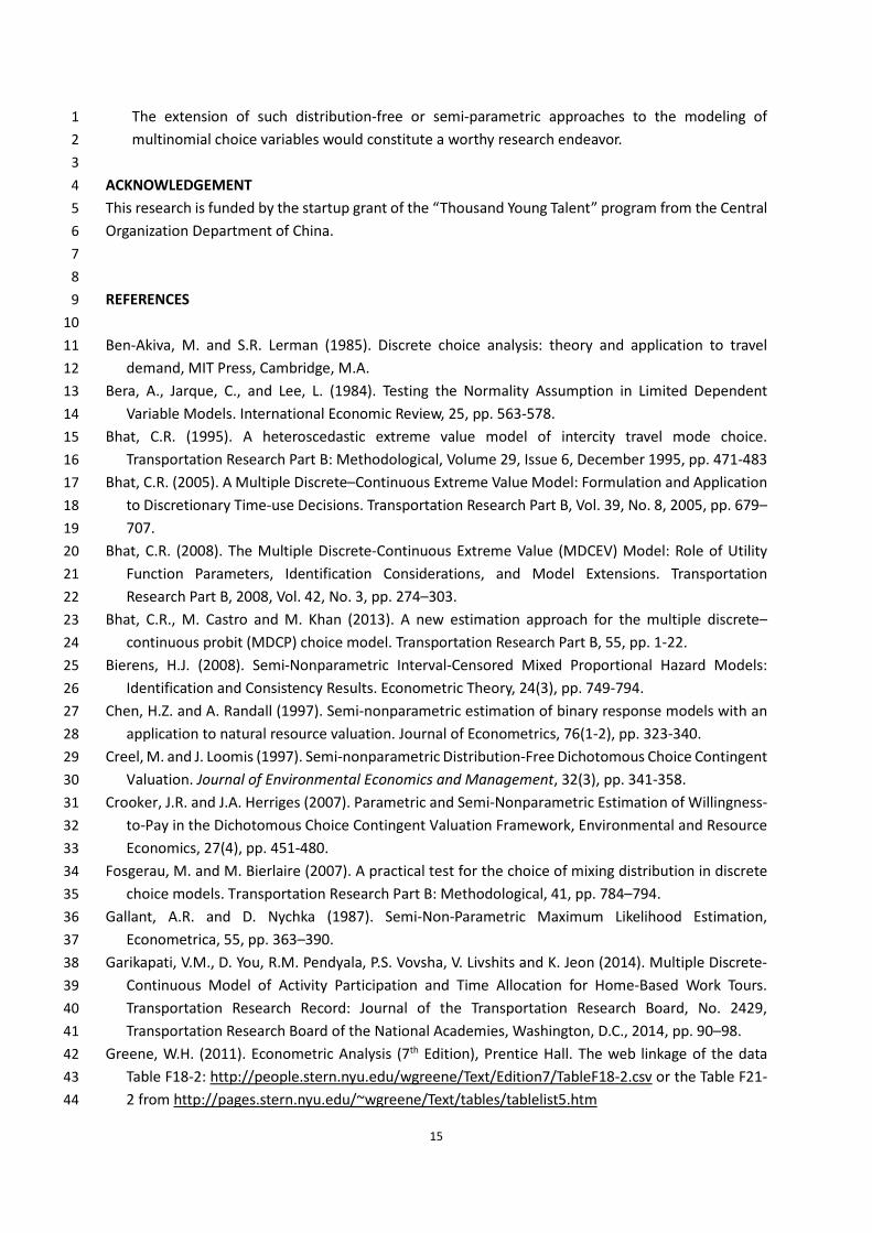
For examining the probability of making Type-II errors, ε1 should follow a distribution other than 37

the standard Gumbel distribution, G(0,1). Two types of normal distributions are chosen for ε1 in this 38

simulation experiment. One is the standard normal distribution, i.e., N(0,1), and the other is a 39

normal distribution adjusted to have the same expectation and standard deviation as that of a 40

standard Gumbel distribution. Figure 1 compares the PDFs of the three distributions. Based on a 41

visual examination, the standard normal distribution seems closer to the standard Gumbel distribution 42

than the adjusted normal distribution. Distributions that are very similar to one another are chosen 43

for this experiment to examine the statistical power of the proposed test. The statistical power can 44

8

be defined as the probability of correctly rejecting the null hypothesis, i.e., P(Reject H0|H0 is wrong), 1

which is equal to [1 - P(Type-II error)]. Through simulation experiments, it is found that the 2

probability of making Type-II errors (or statistical power of the test) depends on both the sample size 3

and how close the erroneous distribution is to the standard Gumbel distribution with respect to 4

expectation and standard deviation. 5

6

Table 1. Simulation Results for MNL models 7

Distribution Sample Size Accepted Rejected

ε1 ~ G(0, 1) 200 1.00 0.00 (Type-I Error)

ε1 ~ G(0, 1) 4000 0.96 0.04 (Type-I Error)

ε1 ~ N(0, 1) 4000 0.03 (Type-II Error) 0.97

ε1 ~ γ + N(0, 1)·�√�

200000 0.02 (Type-II Error) 0.98

γ is the Euler constant ≈ 0.577216; number of repetitions = 100; 0.05 level of significance is used 8

9

10

Figure 1. Comparison of Distributions Being Tested 11

12

A sample size of 4000 is found to be adequate to provide a statistical power of 0.97 and a Type-II 13

error probability less than 0.05 in distinguishing the standard normal distribution from the standard 14

Gumbel distribution. However, when the erroneous distribution is the adjusted normal distribution 15

with the same expectation and standard deviation as that of a standard Gumbel distribution, the 16

sample size needs to be as high as 200000 to obtain satisfactory statistical power and Type-II error 17

probability. Although the standard normal distribution appears more similar (visually) to the 18

standard Gumbel distribution than the adjusted normal distribution, it is actually much more difficult 19

to distinguish the adjusted normal distribution (than the standard normal distribution) from the 20

standard Gumbel distribution presumably because the adjusted normal distribution has the same 21

expectation and standard deviation as the standard Gumbel distribution. 22

23

4.2 Simulation Experiments for Test of MDCEV Model 24

In the MDCEV model specification, either parameter αj or γj needs to be normalized for identification 25

purposes. Alternative normalization approaches will result in two different model profiles, namely, 26

the "α" profile and "γ" profile. Simulation experiments are conducted for both profiles. 27

Similar to previous experiment for the MNL model, the experiment is designed with four 28

alternatives and corresponding random utility values, computed as: 29

9

u1 = -1.0 + 0.9×x1 + ε1; 1

u 2 = -0.6 + 0.8×x2 + ε2; 2

u 3 = -0.7 + 0.4×x3 + ε3; 3

u 4 = 0.6×x4 + ε4. 4

Once again, x1, x2, x3, and x4 follow an independent uniform distribution between 0 and 10, i.e., U(0,10). 5

ε2, ε3, and ε4 follow an independent standard Gumbel distribution, i.e., G(0,1), while ε1 follows either 6

G(0,1) or a distribution other than G(0,1). The continuous resource budget T = Trunc [U(0,1000)]+10, 7

where Trunc[ ] is a function to convert a real number to an integer by truncating its decimal part. The 8

utility function for the α-profile MDCEV model is U* = .p& q* V %�&. + 1'�& − 1W, where q* = y�&, α1 = 9

0.5, α2 = 0.6, α3 = 0.7 and α4 = 0.8. Then, four resource allocation variables, t1, t2, t3, and t4, are 10

calculated by applying the efficient algorithm proposed in Pinjari and Bhat (2011). 11

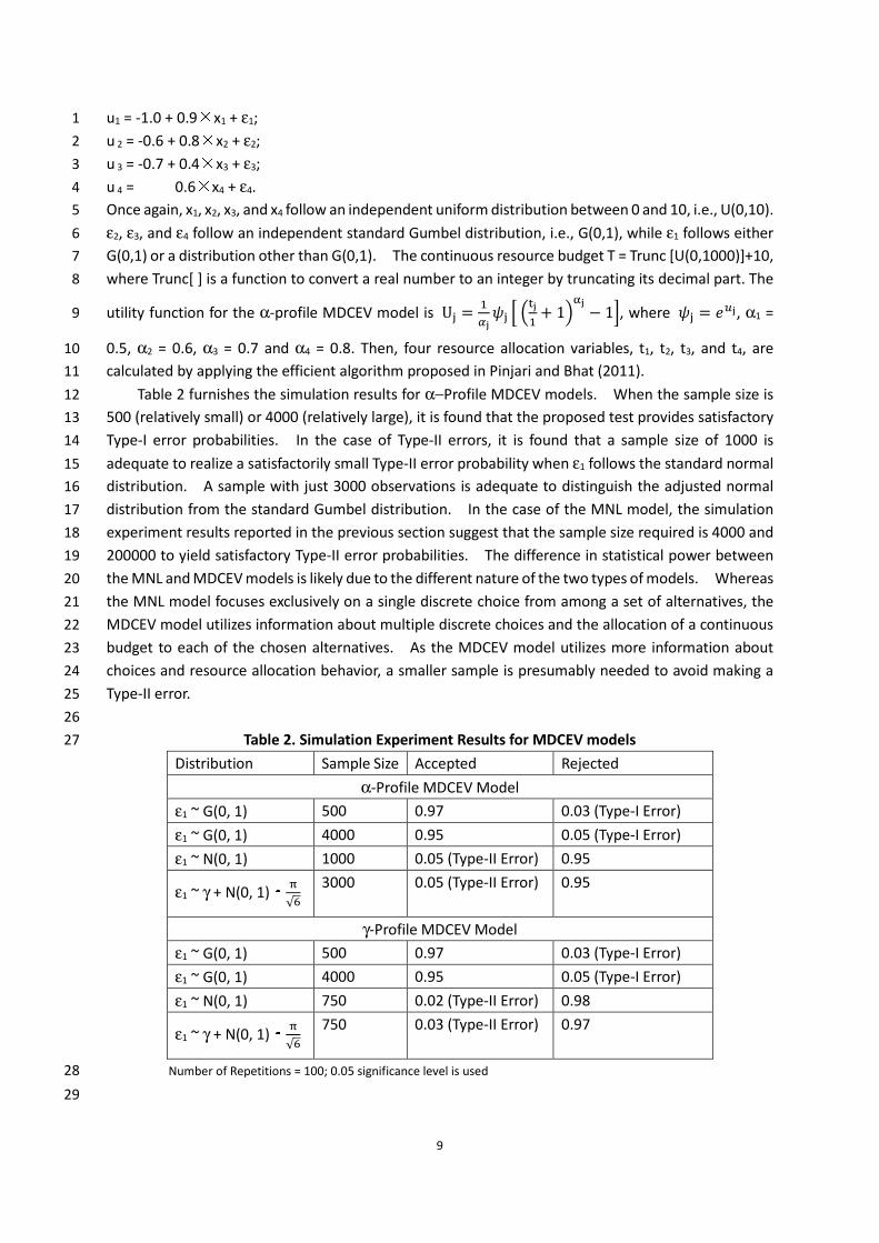
Table 2 furnishes the simulation results for α−Profile MDCEV models. When the sample size is 12

500 (relatively small) or 4000 (relatively large), it is found that the proposed test provides satisfactory 13

Type-I error probabilities. In the case of Type-II errors, it is found that a sample size of 1000 is 14

adequate to realize a satisfactorily small Type-II error probability when ε1 follows the standard normal 15

distribution. A sample with just 3000 observations is adequate to distinguish the adjusted normal 16

distribution from the standard Gumbel distribution. In the case of the MNL model, the simulation 17

experiment results reported in the previous section suggest that the sample size required is 4000 and 18

200000 to yield satisfactory Type-II error probabilities. The difference in statistical power between 19

the MNL and MDCEV models is likely due to the different nature of the two types of models. Whereas 20

the MNL model focuses exclusively on a single discrete choice from among a set of alternatives, the 21

MDCEV model utilizes information about multiple discrete choices and the allocation of a continuous 22

budget to each of the chosen alternatives. As the MDCEV model utilizes more information about 23

choices and resource allocation behavior, a smaller sample is presumably needed to avoid making a 24

Type-II error. 25

26

Table 2. Simulation Experiment Results for MDCEV models 27

Distribution Sample Size Accepted Rejected

α-Profile MDCEV Model

ε1 ~ G(0, 1) 500 0.97 0.03 (Type-I Error)

ε1 ~ G(0, 1) 4000 0.95 0.05 (Type-I Error)

ε1 ~ N(0, 1) 1000 0.05 (Type-II Error) 0.95

ε1 ~ γ + N(0, 1)·�√�

3000 0.05 (Type-II Error) 0.95

γ-Profile MDCEV Model

ε1 ~ G(0, 1) 500 0.97 0.03 (Type-I Error)

ε1 ~ G(0, 1) 4000 0.95 0.05 (Type-I Error)

ε1 ~ N(0, 1) 750 0.02 (Type-II Error) 0.98

ε1 ~ γ + N(0, 1)·�√�

750 0.03 (Type-II Error) 0.97

Number of Repetitions = 100; 0.05 significance level is used 28

29

10

The experiment for γ−profile MDCEV models also considers four alternatives with random utility 1

values computed as: 2

u1 = 0.4 - 0.5×x1 + ε1; 3

u2 = -0.5 - 0.4×x2 + ε2; 4

u3 = -0.6 - 0.3×x3 + ε3; 5

u4 = - 0.5×x4 + ε4. 6

x1, x2, x3, and x4 follow an independent uniform distribution between 0 and 10, i.e., U(0, 10). ε2, ε3, and 7

ε4 follow an independent standard Gumbel distribution, i.e., G(0,1), while ε1 follows either G(0,1) or a 8

distribution other than G(0,1). The continuous resource budget T = Trunc[U(0,500)] + 10. The utility 9

function is U* = x*q*lB r�&o& + 1v, where q* = y�&, γ1 = 2.0, γ2 = 1.0, γ3 = 0.5 and γ4 = 1.5. Four resource 10

allocation variables t1, t2, t3, and t4 are calculated by applying the efficient forecasting algorithm of 11

Pinjari and Bhat (2011). Table 2 provides the simulation experiment results for γ−Profile MDCEV 12

models. 13

Similar to the α-profile MDCEV models, γ-profile MDCEV models have satisfactory Type-I error 14

probabilities when the sample size is 500 (relatively small) and 4000 (relatively large), respectively. 15

As for the statistical power, γ-profile MDCEV models require even fewer observations (750) than the 16

α-profile MDCEV models to distinguish the normal or adjusted normal distribution from the standard 17

Gumbel distribution. 18

19

5. CASE STUDIES 20

The simulation experiments demonstrated the efficacy of the statistical test developed in this research 21

effort. The proposed testing methods were applied to MNL and MDCEV models estimated on real-22

world travel survey data sets to examine the extent to which violations of the standard Gumbel 23

distribution occur in different empirical contexts. 24

25

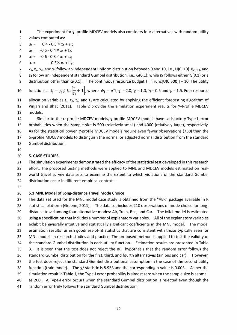
5.1 MNL Model of Long-distance Travel Mode Choice 26

The data set used for the MNL model case study is obtained from the "AER" package available in R 27

statistical platform (Greene, 2011). The data set includes 210 observations of mode choice for long-28

distance travel among four alternative modes: Air, Train, Bus, and Car. The MNL model is estimated 29

using a specification that includes a number of explanatory variables. All of the explanatory variables 30

exhibit behaviorally intuitive and statistically significant coefficients in the MNL model. The model 31

estimation results furnish goodness-of-fit statistics that are consistent with those typically seen for 32

MNL models in research studies and practice. The proposed method is applied to test the validity of 33

the standard Gumbel distribution in each utility function. Estimation results are presented in Table 34

3. It is seen that the test does not reject the null hypothesis that the random error follows the 35

standard Gumbel distribution for the first, third, and fourth alternatives (air, bus and car). However, 36

the test does reject the standard Gumbel distributional assumption in the case of the second utility 37

function (train mode). The χ2 statistic is 8.933 and the corresponding p-value is 0.003. As per the 38

simulation result in Table 1, the Type-I error probability is almost zero when the sample size is as small 39

as 200. A Type-I error occurs when the standard Gumbel distribution is rejected even though the 40

random error truly follows the standard Gumbel distribution. 41

11

Table 3. Test Results of the MNL model (N = 210)

Model MNL Model Test (Air Utility) Test (Train Utility) Test (Bus Utility) Test (Car Utility)

Variable Coeff. t-test Coeff. t-test Coeff. t-test Coeff. t-test Coeff. t-test

Constant for Air 8.038 5.58 7.822 4.86 7.618 5.39 7.955 5.54 6.425 4.35

Air travel time (min) -0.030 -4.18 -0.031 -4.20 -0.031 -4.50 -0.030 -4.17 -0.024 -3.40

Party size in mode choice -0.951 -3.66 -0.962 -3.62 -0.864 -3.45 -0.937 -3.62 -0.837 -3.49

Air waiting time (min) -0.103 -5.72 -0.105 -5.75 -0.101 -5.69 -0.103 -5.71 -0.094 -5.41

δ1 -- -- 0.133 0.40 -- -- -- -- -- --

Constant for Train 4.409 5.03 4.429 5.04 4.253 6.45 4.349 4.98 3.185 3.61

Train travel time (min) -0.005 -2.94 -0.005 -2.99 -0.005 -3.80 -0.005 -2.97 -0.004 -2.55

Train cost ($) -0.024 -1.84 -0.024 -1.85 -0.019 -2.04 -0.024 -1.83 -0.021 -1.75

Household annual income (K $) -0.048 -3.66 -0.048 -3.65 -0.036 -3.96 -0.047 -3.62 -0.042 -3.45

Train waiting time (min) -0.064 -3.83 -0.064 -3.82 -0.045 -4.17 -0.064 -3.80 -0.058 -3.64

δ1 -- -- -- -- -0.745 -3.43 -- -- -- --

Constant for Bus 4.905 3.85 4.919 3.86 4.461 3.68 5.033 4.19 3.643 2.88

Bus travel time (min) -0.006 -3.26 -0.006 -3.30 -0.006 -3.55 -0.006 -3.40 -0.004 -2.29

Bus waiting time (min) -0.151 -5.17 -0.151 -5.16 -0.141 -5.09 -0.138 -4.13 -0.147 -5.18

δ1 -- -- -- -- -- -- -0.195 -1.07 -- --

Car travel time (min) -0.006 -5.13 -0.007 -5.14 -0.007 -5.70 -0.006 -5.15 -0.005 -3.68

δ1 -- -- -- -- -- -- -- -- -0.588 -1.16

LL(β) -160.092 -- -159.963 -- -155.626 -- -159.751 -- -159.339 --

χ2 Statistic -- -- 0.258 -- 8.933 -- 0.683 -- 1.506 --

p-value -- -- 0.611 -- 0.003 -- 0.409 -- 0.220 --

12

Therefore, it can be concluded that the standard Gumbel distribution is not valid for the random error 1

term in the utility equation of the train mode. It is also interesting to see that the additional coefficient 2

"δ1" is significant and considerably changes the magnitude of coefficients in the second utility function. 3

4

5.2 MDCEV Model of Activity Engagement and Time Allocation 5

The proposed method is next applied to an MDCEV model of activity (stop) engagement and time 6

allocation for home-based work tours, where the primary purpose of the tour is to go to the workplace. 7

The model predicts the secondary activities that will be undertaken during the tour, along with the 8

time allocated to each activity. The model is estimated on 2009 National Household Travel Survey 9

(NHTS) data from the Greater Phoenix Metropolitan Area (Garikapati et al. 2014). In the interest of 10

brevity, model estimation results are suppressed in this paper. Activities within a home-based work 11

tour are classified into 11 types. Explanatory variables include commuters' demographic and socio-12

economic characteristics, commute and work status, built environment attributes associated with 13

residential and work locations, and accessibility measures. The sample size of the estimation sample 14

is 1968 and the log-likelihood value at convergence is -17528.658. 15

The proposed method is applied to test the validity of the standard Gumbel distribution for the 16

random error term in the utility function of each activity type. The test results, including the log-17

likelihood value at convergence, χ2 statistics and corresponding p-values, are listed in Table 4. It is 18

seen that the likelihood ratio tests reject the distributional assumption for all of the utility functions in 19

the MDCEV model. It is interesting to see that the χ2 statistic values for two outside goods (going to 20

work and returning home) are considerably lower than those for other goods, which implies that the 21

distributional assumption is even more invalid for alternatives that are not outside goods. Outside 22

goods are those that are consumed (chosen) by all observations in the data set. In this case, going to 23

work and returning home are activities that must be undertaken in the context of home-based work 24

tours and are therefore treated as outside goods. 25

26

Table 4. Test Results for the MDCEV Model of Home-Based Work Tour 27

Activity Engagement and Time Allocation 28

Activity Type LL(b) χ2 Statistics p-value

Work Epoch (outside good 1) -17218.635 620.047 0.000

Home Epoch (outside good 2) -17377.888 301.539 0.000

Other Escort Epoch 1 -14957.450 5142.417 0.000

Other Escort Epoch 2 -14871.097 5315.122 0.000

School Escort Epoch 1 -14987.671 5081.973 0.000

School Escort Epoch 2 -14860.288 5336.741 0.000

Shopping Epoch 1 -15118.892 4819.533 0.000

Maintenance Epoch 1 -15071.536 4914.243 0.000

Meal Epoch 1 -14987.993 5081.330 0.000

Social Visit Epoch 1 -14850.375 5356.567 0.000

Other Discretionary Epoch 1 -14925.381 5206.554 0.000

29

5.3 MDCEV Model of Household Vehicle Fleet Composition and Utilization 30

The proposed method is finally applied to a MDCEV model of household vehicle fleet composition and 31

utilization. The model was estimated on 2009 National Household Travel Survey (NHTS) data from 32

13

the Greater Phoenix Metropolitan Area (You et al. 2014). Model estimation results are suppressed in 1

the interest of brevity. Household vehicles are categorized into 14 types, defined by a cross-2

classification of body type and vintage. Explanatory variables include household composition and 3

structure, economic status, and built environment attributes of the household location. The estimation 4

sample has 4262 observations and the log-likelihood value at convergence is -77020.486. 5

The proposed method is applied to test the validity of the standard Gumbel distribution for the 6

random error term in the utility function of each vehicle type. Results of the test are shown in Table 7

5. It is seen once again that the likelihood ratio tests reject the distributional assumption for all utility 8

functions of the MDCEV model. As in the previous case, the χ2 statistic for the outside good is much 9

lower than those for other goods, which implies that the distributional assumption is more invalid for 10

alternatives that are not treated as outside goods. In this model, non-motorized vehicle is treated as 11

the outside good as all individuals are assumed to walk for at least some minimal duration over the 12

course of a day. Thus, the non-motorized vehicle is chosen by all observations in the data set. 13

14

Table 5. Test Results for the MDCEV Model of Vehicle Fleet Composition and Utilization 15

Vehicle Type LL(b) Chi-Sq. Statistics p-value

Non-motorized vehicle

(outside good) -76839.481 362.018 0.000

Car (years) 0–5 -73185.231 7670.517 0.000

6–11 -72898.926 8243.128 0.000

≥12 -72234.349 9572.282 0.000

Van (years) 0–5 -71472.336 11096.308 0.000

6–11 -71493.089 11054.802 0.000

≥12 -71239.748 11561.484 0.000

SUV (years) 0–5 -72159.229 9722.522 0.000

6–11 -71842.624 10355.732 0.000

≥12 -71363.351 11314.278 0.000

Pickup (years) 0–5 -71736.722 10567.536 0.000

6–11 -71832.517 10375.946 0.000

≥12 -71591.310 10858.360 0.000

Motorbike -71387.042 11266.896 0.000

16

6. CONCLUSIONS AND DISCUSSIONS 17

In this paper, a practical but statistically rigorous method is proposed to test the validity of the standard 18

Gumbel distribution assumption that is often associated with the random error components in 19

multinomial travel-related choice models, including both discrete and discrete-continuous models. 20

The method is based on the use of the orthonormal Legendre polynomial to derive a closed-form 21

likelihood expression that nests the likelihood functions of the multinomial logit (MNL) and multiple 22

discrete-continuous extreme value (MDCEV) models. The standard likelihood-ratio test can then be 23

applied to test the validity of the Gumbel distribution innate to the logit-based choice models. The 24

efficacy of the proposed method is first examined via simulation experiments. Results of the 25

simulation experiments show that acceptably low Type-I and Type-II error probabilities in the 26

application of the test may be realized at typically available travel survey sample sizes, except for the 27

case of the Type-II error probability for the multinomial logit model (which needs a sample size on the 28

14

order of 200000 to ensure Type-II error probability less than 0.05). The proposed method is then 1

applied to three real-world case studies, including a multinomial logit model of long-distance travel 2

mode choice, a multiple discrete-continuous choice model of activity-time allocation in home-based 3

work tours, and another multiple discrete-continuous choice model of vehicle fleet composition and 4

utilization. For all three models, the proposed test shows that the assumption of a standard Gumbel 5

distribution for the random error components is rejected at a high level of confidence. 6

In theory, the violation of underlying distributional assumptions will lead to the estimation of 7

parameters that are statistically inconsistent and inefficient. However, the extent to which departures 8

from the standard Gumbel distribution affect the magnitudes of model coefficients and model 9

sensitivity to policy scenarios remains unclear. This question could be addressed in future research 10

using simulation experiments in which a robust model based on valid distributional assumptions is 11

developed. Then, the impacts of modifying the distribution on the random error component on 12

parameter estimates in logit-based models can be explicitly quantified. 13

The three real-world models considered in this paper are typical discrete or discrete-continuous 14

choice models with a rich set of explanatory variables and exhibiting goodness-of-fit statistically 15

typically encountered in practice. Given that violations of the standard Gumbel distribution are 16

occurring even in the context of these models, it is prudent to identify approaches that could 17

potentially overcome any ill-effects of the distributional assumption violations. Three strategies are 18

noted below: 19

1. Adopting an alternative parametric distribution 20

The normal distribution is usually a preferred distribution for the error term that captures the 21

effects of unobserved factors (as opposed to the Gumbel distribution). Thus, the corresponding 22

multinomial probit (MNP) or multiple discrete-continuous probit (MDCP) models (Bhat et al., 2013) 23

are likely to be better alternatives to MNL and MDCEV models. In addition, heteroskedastic 24

versions of the logit model or discrete-continuous choice model (Bhat, 1995; Sikder and Pinjari, 25

2013) may also prove to be better alternatives. However, tests should be conducted to determine 26

whether violations of the chosen alternative parametric distribution are occurring. There are 27

methods currently available to test for violations of the normal distribution in the econometric 28

literature (e.g., Bera et al., 1984). 29

2. Adopting mixed logit model with random coefficients of known distribution 30

Modelers may still use the standard Gumbel distribution for the random error components, but 31

could identify a random coefficient that follows a certain parametric distributional assumption. 32

Then, this coefficient may be scaled up to approximate the random utility values and minimize the 33

impact of the Gumbel random disturbance. Details of this method are described in Train (2009). 34

Note that the existence of such a random coefficient is a necessary condition to apply this method. 35

The test proposed by Fosgerau and Bierlaire (2007) may be used to test the distributional 36

assumption on a random coefficient in a mixed logit model. 37

3. Developing a robust multinomial choice model free from distributional assumptions 38

Statistical or econometric models estimated using maximum likelihood methods necessarily 39

involve the making of distributional assumptions. Modelers have longed for the development of 40

robust choice models free from distributional assumptions for several decades (e.g., Manski, 1975; 41

Gallant and Nychka, 1987; Klein and Spady, 1993); however, most practical distribution-free or 42

semi-parametric choice methods have been limited to the analysis and modeling of binary choice 43

variables, rendering their application to multinomial choice contexts computationally challenging. 44

15

The extension of such distribution-free or semi-parametric approaches to the modeling of 1

multinomial choice variables would constitute a worthy research endeavor. 2

3

ACKNOWLEDGEMENT 4

This research is funded by the startup grant of the “Thousand Young Talent” program from the Central 5

Organization Department of China. 6

7

8

REFERENCES 9

10

Ben-Akiva, M. and S.R. Lerman (1985). Discrete choice analysis: theory and application to travel 11

demand, MIT Press, Cambridge, M.A. 12

Bera, A., Jarque, C., and Lee, L. (1984). Testing the Normality Assumption in Limited Dependent 13

Variable Models. International Economic Review, 25, pp. 563-578. 14

Bhat, C.R. (1995). A heteroscedastic extreme value model of intercity travel mode choice. 15

Transportation Research Part B: Methodological, Volume 29, Issue 6, December 1995, pp. 471-483 16

Bhat, C.R. (2005). A Multiple Discrete–Continuous Extreme Value Model: Formulation and Application 17

to Discretionary Time-use Decisions. Transportation Research Part B, Vol. 39, No. 8, 2005, pp. 679–18

707. 19

Bhat, C.R. (2008). The Multiple Discrete-Continuous Extreme Value (MDCEV) Model: Role of Utility 20

Function Parameters, Identification Considerations, and Model Extensions. Transportation 21

Research Part B, 2008, Vol. 42, No. 3, pp. 274–303. 22

Bhat, C.R., M. Castro and M. Khan (2013). A new estimation approach for the multiple discrete–23

continuous probit (MDCP) choice model. Transportation Research Part B, 55, pp. 1-22. 24

Bierens, H.J. (2008). Semi-Nonparametric Interval-Censored Mixed Proportional Hazard Models: 25

Identification and Consistency Results. Econometric Theory, 24(3), pp. 749-794. 26

Chen, H.Z. and A. Randall (1997). Semi-nonparametric estimation of binary response models with an 27

application to natural resource valuation. Journal of Econometrics, 76(1-2), pp. 323-340. 28

Creel, M. and J. Loomis (1997). Semi-nonparametric Distribution-Free Dichotomous Choice Contingent 29

Valuation. Journal of Environmental Economics and Management, 32(3), pp. 341-358. 30

Crooker, J.R. and J.A. Herriges (2007). Parametric and Semi-Nonparametric Estimation of Willingness-31

to-Pay in the Dichotomous Choice Contingent Valuation Framework, Environmental and Resource 32

Economics, 27(4), pp. 451-480. 33

Fosgerau, M. and M. Bierlaire (2007). A practical test for the choice of mixing distribution in discrete 34

choice models. Transportation Research Part B: Methodological, 41, pp. 784–794. 35

Gallant, A.R. and D. Nychka (1987). Semi-Non-Parametric Maximum Likelihood Estimation, 36

Econometrica, 55, pp. 363–390. 37

Garikapati, V.M., D. You, R.M. Pendyala, P.S. Vovsha, V. Livshits and K. Jeon (2014). Multiple Discrete-38

Continuous Model of Activity Participation and Time Allocation for Home-Based Work Tours. 39

Transportation Research Record: Journal of the Transportation Research Board, No. 2429, 40

Transportation Research Board of the National Academies, Washington, D.C., 2014, pp. 90–98. 41

Greene, W.H. (2011). Econometric Analysis (7th Edition), Prentice Hall. The web linkage of the data 42

Table F18-2: http://people.stern.nyu.edu/wgreene/Text/Edition7/TableF18-2.csv or the Table F21-43

2 from http://pages.stern.nyu.edu/~wgreene/Text/tables/tablelist5.htm 44

16

Jäggi, B., C. Weis and K.W. Axhausen (2013). Stated response and multiple discrete-continuous choice 1

models: Analyses of residuals. Journal of Choice Modelling, 6, pp. 44-59. 2

Klein, R.W. and R.H. Spady (1993). An Efficient Semiparametric Estimator for Binary Response Models. 3

Econometrica, 61(2), pp. 387-421. 4

Lee, L.F. (1995). Semiparametric maximum likelihood estimation of polychotomous and sequential 5

choice models. Journal of Econometrics, 65, pp. 381-428 6

Manski, C.F. (1975). Maximum score estimation of the stochastic utility model of choice. Journal of 7

Econometrics, 3(3), pp. 205–228. 8

Mcfadden, D. (1974). Conditional logit analysis of qualitative choice behavior. in P. Zarembka (ed.), 9

Frontiers in Econometrics, pp. 105-142, Academic Press: New York. 10

Pinjari, A.R. and C.R. Bhat (2011). Computationally efficient forecasting procedures for Kuhn-Tucker 11

consumer demand model systems: application to residential energy consumption analysis. 12

Technical paper, Department of Civil and Environmental Engineering, University of South Florida. 13

Sikder, S. and A.R. Pinjari (2013). The benefits of allowing heteroscedastic stochastic distributions in 14

multiple discrete-continuous choice models. Journal of Choice Modelling, 9, pp. 39-56. 15

Train, K.E. (2009). Discrete choice methods with simulation. Cambridge University Press. 16

You, D., V.M. Garikapati, R.M. Pendyala, C.R. Bhat, S. Dubey, K. Jeon, and V. Livshits (2014). 17

Development of Vehicle Fleet Composition Model System for Implementation in Activity-Based 18

Travel Model. Transportation Research Record: Journal of the Transportation Research Board, No. 19

2430, pp. 145–154. 20

21

22

23

24

25

26

27

28

29

17

Appendix A: Mathematical Derivation of the Test for MNL Model 1

Suppose there are "J" alternatives in the choice set and their random utility functions are U1, U2, ..., UJ. And 2

the utility Uj is expressed as the sum of the systematic component Vj and the random component εj , i.e. Uj 3

= Vj + εj. Suppose the standard Gumbel distributional assumption of ε1 needs to be tested. All the other 4

εj (j > 1) really follow the standard Gumbel distribution. One can derive the probability that the alternative 5

1 is chosen as: 6 i�k = 1� = i��. > �6 , �. > �8 , … , �. > �� � 7 = i��. + ε. > �6 + ε6, �. + ε. > �8 + ε8, … , �. + ε. > �� + εm� 8 = i�ε6 < �.6 + ε., ε8 < �.8 + ε., … , εm < �.� + ε.�. 9

In the formulae above, Vij represents Vi - Vj. Since εj are assumed to be independently distributed in an 10

MNL model, then i�k = 1� = � V∏ G�V.* + ε.�m*[6 W#∞$∞ f�ε.�"ε.. 11

By plugging the PDF of the semi-nonparametric distribution in Equation (9), one can obtain that 12

i�k = 1� = � V∏ G�V.* + ε.�m*[6 W S∑ ξY[Z�ε.�]:6Y[- U#∞$∞ g�ε.�"ε.. 13

Then, it can be simplified as i�k = 1� = ∑ ξ:6:[- e.�@�, where 14

e.�@� = � V∏ G�V.* + ε.�m*[6 W [G�ε.�]Y#∞$∞ g�ε.�"ε. 15

= � V∏ exp�−e$zJ&$ �J�m*[6 W [exp�−e$ �J�]Y#∞$∞ exp�−e$ �J�exp �− ε.�"ε. 16

= − � V∏ exp�−e$zJ&$ �J�m*[6 W [exp�−e$ �J�]Y#∞$∞ exp�−e$ �J�"[exp �− ε.�]. 17

Let � = exp�− ε.�. Since ε1 ranges from -∞ to +∞, "w" should range from +∞ to 0. Then 18

e.�@� = − � V∏ exp�−w · e$zJ&�m*[6 W [exp�−w�]Y-#∞ exp�−w�"w 19

= − � exp �−� ∑ e$zJ&��[6 − @� − ��-#∞ "w. 20

Let � = − ∑ e$zJ&��[6 − @ − 1, then e.�@� = − � exp ����-#∞ "w = − .� � exp ����-#∞ "����. 21

Let η = θw. Since "w" ranges from +∞ to 0 and θ < 0, η should range from -∞ to 0. Then, e.�@� =22

− .� � exp ���-$∞ "� = − .� = − .$ ∑ g�(J&���� $:$. = .∑ g(&�(J���� #:#. = ��J�:#.���J#∑ ������� = ��J

:·��J#∑ ������J . 23

For the alternative other than the 1st one (say the 2nd alternative), its choice probability: 24 i�k = 2� = i��6 > �. , �6 > �8 , … , �6 > �� � 25 = i��6 + ε6 > �. + ε., �6 + ε6 > �8 + ε8, … , �6 + ε6 > �� + εm� 26 = i�ε. < �6. + ε6, ε8 < �68 + ε6, … , εm < �6� + ε6�. 27

Since ]�ε.� = ∑ bξY [`��J�]��JY#. d6Y[- according to Equation (10), i�k = 2� =28

� ∑ bξY [`���J#���]��JY#. d6Y[- V∏ G�V6* + ε6�m*[8 W#∞$∞ g�ε6�"ε6. It can be simplified as 29

i�k = 2� = ∑ ξYq6�m�6:[- , where 30

18

e6�@� = .:#. � [Z��6. + ε6�]:#. V∏ G�V6* + ε6�m*[8 W#∞$∞ g�ε6�"ε6 1

= .:#. � y;��−y$��J$��#�3 �Y#.�� V∏ y;��−y$���$���m*[8 W#∞$∞ exp �−e$��� · e$��"ε6 2

= − .:#. � y;��−y$��J$��#�3 �Y#.�� V∏ y;��−y$���$���m*[8 W#∞$∞ exp �−e$���"e$�� 3

Let � = e$��. Since ε2 ranges from -∞ to +∞, “w” should range from +∞ to 0, then 4

e6�@� = − .:#. � y;��−� · y$��J#�3 �Y#.�� V∏ y;��−� · y$����m*[8 W-#∞ exp �−w�"w 5

= − .:#. � y;��−� · y$��J#�3 �Y#.���y;��−� · ∑ y$�����[8 ��-#∞ exp �−w�"w. 6

Let θ = −y$��J#�3 �Y#.� − ∑ y$�����[8 − 1, then 7

e6�@� = − .:#. � exp �θw�-#∞ "w = − . �Y#.� � exp �θw�-#∞ "�θw�. 8

Let η = θw. Since “w” ranges from +∞ to 0 and θ < 0, η should range from -∞ to 0. Then, 9

e6�@� = − . �Y#.� � exp �η�-$∞ "�η� = − . �Y#.� = .:#. · .����J�¢£ �a�J�#∑ ��������¤ #. 10

= .:#. · ����:#.�·��J#∑ ������¤ #��� = ���

�:#.�%:·��J#∑ ������J '. 11

Without loss of generality, e¦�@� = ��§�:#.�%:·��J#∑ ������J ' , where k > 1. 12

13

14

Appendix B: Mathematical Derivation of the Test for MDCEV Model 15

Assume the utility for the alternative "j" takes the following form as in Bhat (2008): �� =16

o�p� q� r st�o� + 1up� − 1v, where q� = y��#�� and the alternative index j = 1, 2,..., K. Suppose the random 17

error ε. in the 1st alternative needs to be tested. "K" represents the total number of alternatives and 18

"M" represents the total number of alternatives being allocated resource (M ≤ K). Each individual is 19

supposed to allocate continuous resource by maximizing the overall utility value subject to the budget: 20

Maximize ∑ o�p� q� r st�o� + 1up� − 1vª�[. subject to ∑ «� = ¬ª�[. . 21

It is equivalent to maximizing ∑ o�p� q� r st�o� + 1up� − 1vª�[. − ­�∑ «� − ¬ª�[. �. For the observation where 22

the resource allocation t1 > 0, according to KT conditions, one should have 23

q. %tJoJ + 1'pJ$. = ­ , q6 %t�o� + 1'p�$.

= ­ , ..., q® %to¯ + 1'p¯$. = ­ ; q®#. %t¯�Jo¯�J + 1'p¯�J$.

< 24

­ ,..., qª %t±o± + 1'p±$. < ­. 25

In the above formulae, tj > 0 when j ≤ M and tj = 0 when M < j ≤ K. Then, one will have 26

q. %tJoJ + 1'pJ$. = q� st�o� + 1up�$.

，j = 2, 3, ..., M. 27

19

Take a logarithm function on both sides and one should obtain that: 1 �. + !. = �� + !�，j = 2, 3, ..., M; 2

�. + !. > �� + !�，j = (M+1), (M+2), ..., K, where �� = ;�²� + �w� − 1�ln st�o� + 1u. 3

As per Bhat (2005), the likelihood value i = |¶| · � �∏ ·��.� + !.�®�[6 ��∏ Z��.� + !.�ª�[®#. ���!.�"!.R$R . 4

To obtain ��!.� , one can plug the SNP density function: ��;� = S∑ ξY[Z�;�]:6Y[- Ug�x� into the 5

equation above and then have that i = |¶| � �∏ ·��.� + !.�®�[6 ��∏ Z��.� +ª�[®#.R$R6

!.��S∑ ξY[Z�!.�]:6Y[- Ug�!.�"!. 7

= ∑ j:|¶| � �∏ ·��.� + !.�®�[6 ��∏ Z��.� + !.�ª�[®#. �[Z�!.�]:g�!.�"!.R$R6:[- = ∑ j:e.�@�6:[- , 8

where e.�@� = � |¶|�∏ ·��.� + !.�®�[6 ��∏ Z��.� + !.�ª�[®#. �[Z�!.�]:g�!.�"!.#∞$∞ 9

=|¶| � �∏ ·��.� + !.�®�[6 ��∏ Z��.� + !.�ª�[®#. �FZ(!.)I:g(!.)"!.R$R 10

=|¶| � C∏ �Z��.� + !.� · y$�J�$¸J�®�[6 K�∏ Z��.� + !.�ª�[®#. �FZ(!.)I:Z(!.)y$¸J"!.R$R 11

=|¶| � C∏ �Z��.� + !.� · y$�J�$¸J�®�[6 K�∏ Z��.� + !.�ª�[®#. �FZ(!.)I:Z(�.. + !.)y$¸J"!.R$R 12

= |¶| � ∏ Z��.� + !.�ª�[. �∏ y$�J�$¸J®�[6 �FZ(!.)I:y$¸J"!.R$R 13

= |¶| � �∏ y;�(−y$�J�$¸J)ª�[. ��∏ y$�J�®�[6 �(y$¸J)®$.y$¸J · FZ(!.)I:"R$R !. 14

= |¶|�∏ y$�J�®�[6 � � y;��− ∑ y$�J�$¸Jª�[. �(y$¸J)®$.y;��−y$¸J#¹<(:)�y$¸J"!.#∞$∞ 15

Define the integral part in the formula above as "ºB«": 16

ºB« = � y;��− ∑ y$�J�$¸Jª�[. �(y$¸J)®$.y;��−y$¸J#¹<(:)�y$¸J"!.#∞$∞ 17

= − � y;��− ∑ y$�J�$¸Jª�[. �(y$¸J)®$.y;��−y$¸J#¹<(:)�"y$¸J#∞$∞ 18

Let w = y$¸J. Since !. ranges from −∞ to +∞, w should range from +∞ to 0. Then, 19

ºB« = − � y;��−� ∑ y$�J�ª�[. ��®$.y;�(−@�)"�-#∞ 20

= − � y;��−��∑ y$�J�ª�[. + @���®$."�-#∞ . 21

Let » = ∑ y$�J�ª�[. + @ and ºB« = − � exp (−� · »)�®$."�-#∞ . Let ¼ = −»� , then � = − ½¾ and 22

"� = − ¿½¾ . Since "w" ranges from +∞ to 0 and a > 0, "b" should range from −∞ to 0. Thus, ºB« =23

− � e½ %− ½¾'®$. %− .

¾'-$R "¼ = ($.)¯�J¾¯ � e½ · ¼®$.-$R "¼. 24

As per Bhat (2005), � eÀ · b}$."b = (−1)}$. · (M − 1)!-$R . Then, ºB« = ($.)¯�J¾¯ (−1)}$. · (M −25

20

1)! = (®$.)!¾¯ = (®$.)!

%:#∑ ���J�±��J '¯ · 1

Then, e.(@) = |¶|�∏ y$�J�®�[6 � �®$.�!%:#∑ ���J�±��J '¯ = |¶|�∏ y$�J#��®�[6 � �®$.�!

%:#∑ ���J���±��J '¯ 2

= |¶|( − 1)! %∏ �����J '%:·��J#∑ ���±��J '¯. 3

As per page 704 in Bhat (2005), |¶| = �∏ c*}*[. � s∑ .~&

}*[. u , where c* = .$�&�&#o� . Thus, e.(@) =4

�∏ c*}*[. � s∑ .~&

}*[. u à ∏ �����J%:·��J#∑ ���±��J '¯Ä ( − 1)!. 5

For the observation where the resource allocation t1 = 0, one may pick out another alternative (say "2") 6

to which the resource is allocated and therefore t2 > 0. According to KT conditions, 7

�6 + !6 = �� + !�，j = 3, ..., (M+1); 8

�6 + !6 > �. + !.; 9

�6 + !6 > �� + !�，j = (M+2), (M+3), ..., K. 10

The likelihood value can be computed as: 11

i = |¶| · � �∏ ·��6� + !6�®#.�[8 �]��6. + !6��∏ Z��6� + !6�ª�[®#6 �·�!6�"!6R$R . 12

Here, the CDF of the SNP distribution, as in Equation (10), is used for F(x). Then, i = |¶| ·13

� �∏ ·��6� + !6�®#.�[8 � ∑ bca[`���J#¸��]��JY#. d6Y[- �∏ Z��6� + !6�ª�[®#6 �·�!6�"!6R$R 14

= ∑ ξY6Y[- |m|Y#. � �∏ ·��6� + !6�®#.�[8 �[Z��6. + !6�]:#.�∏ Z��6� + !6�ª�[®#6 �·�!6�"!6R$R . 15

Let e6�@� = |m|Y#. � �∏ ·��6� + !6�®#.�[8 �[Z��6. + !6�]:#.�∏ Z��6� + !6�ª�[®#6 �·�!6�"!6R$R and 16

i = ∑ ξY6Y[- q6�m�. Then, let e6�@� = |m|Y#. ºB«1 , where 17

ºB«1 = � �∏ ·��6� + !6�®#.�[8 �[Z��6. + !6�]:#.�∏ Z��6� + !6�ª�[®#6 �·�!6�"!6R$R . 18

= � �∏ Z��6� + !6�®#.�[8 ��∏ y;��−�6� − !6�®#.�[8 �[Z��6. + !6�]:#.�∏ Z��6� + !6�ª�[®#6 �Z��66 +R$R19

!6�exp �−!6�"!6 20

= � �∏ Z��6� + !6�ª�[6 ��∏ y;��−�6� − !6�®#.�[8 �[Z��6. + !6�]:#.exp �−!6�"!6R$R 21

= � �∏ exp �− y$���$¸��ª�[6 ��∏ y;��−�6��®#.�[8 ��y$¸��®$. · [Z��6. + !6�]:#. · exp �−!6�"!6R$R 22

= �∏ y;��−�6��®#.�[8 � � �∏ exp �− y$���$¸��ª�[6 ��y$¸��®$. · [Z��6. + !6�]:[Z��6. + !6�]. ·R$R23

exp �−!6�"!6 24

= �∏ y;��−�6��®#.�[8 � � �∏ exp �− y$���$¸��ª�[6 ��y$¸��®$. · [Z��6. + !6�]:exp �−y$��J$¸�� ·R$R25

exp �−!6�"!6 26

21

= �∏ y;��−�6��®#.�[8 � � �∏ exp �− y$���$¸��ª�[. ��y$¸��®$. · [Z��6. + !6�]: · e$¸�"!6R$R 1

= �∏ y;��−�6��®#.�[8 �ºB«2, where 2

ºB«2 = � �∏ exp �− y$���$¸��ª�[. ��y$¸��®$. · [Z��6. + !6�]: · e$¸�"!6R$R 3

= � �∏ exp �− y$���$¸��ª�[. ��y$¸��®$. · exp �−y$¸�$��J#�3 �:�� · e$¸�"!6R$R 4

= � exp �−y$¸� ∑ y$���ª�[. ��y$¸��®$. · exp �−y$¸�y$��J#�3 �:�� · e$¸�"!6R$R 5

= − � exp �−y$¸� ∑ y$���ª�[. ��y$¸��®$. · exp �−y$¸�y$��J#�3 �:��"e$¸�R$R 6

Let w = e$¸�. Since !6 ranges from −∞ to +∞, w should range from +∞ to 0. Thus, 7

ºB«2 = − � exp �−� ∑ y$���ª�[. ��®$. · exp�−� · y$��J#�3 �:��"w-#R 8

= − � expC−��y$��J#�3 �:� + ∑ y$���ª�[. �K�®$."w-#R . 9

Let » = y$��J#�3 �:� + ∑ y$���ª�[. and then ºB«2 = − � e$¾Æ�®$."w-#R . Let ¼ = −»� , then � =10

− ½¾ , "� = − ¿½¾ . Let ºB«2 = − � e½ %− ½¾'®$. %− .¾'-$R "¼ = �$.�¯�J¾¯ � e½ · ¼®$.-$R "¼ . As per Bhat 11

(2005), � eÀ · b}$."b = �−1�}$. · �M − 1�!-$R . Then, ºB«2 = �$.�¯�J¾¯ �−1�}$. · �M − 1�! = �®$.�!¾¯ · 12

Thus, e6�@� = |m|Y#. �∏ y;��−�6��®#.�[8 � �®$.�!¾¯ 13

= |m|Y#. �∏ y;��−�6��®#.�[8 � �®$.�!%����J�¢£ ���#∑ �����±��J '¯ = |m|�®$.�!�Y#.� V∏ �����¯�J��¤ W

%:����J#∑ �����±��J '¯ 14

= |m|�®$.�!�Y#.� V∏ ���¯�J��¤ W������¯�J%:��J#∑ ���±��J '¯������¯ = |m|�®$.�!�Y#.� ∏ ���¯�J���

%:��J#∑ ���±��J '¯ 15

= �∏ c*}*[. � s∑ .~&}*[. u �®$.�!�Y#.� ∏ ���¯�J���

%:��J#∑ ���±��J '¯. 16

Since t1 = 0, y�J will not be multiplied with the numerator term. However, the numerator term is still the 17

product of exponentials of utilities for "M" alternatives being allocated resource. In summary, the SNP 18

likelihood function can be expressed as i = ∑ ξY6Y[- q�m�, where 19

q�m� =ÇÈÉÈÊ �∏ c*}*[. � s∑ .~&

}*[. u à ∏ �����J%:·��J#∑ ���±��J '¯Ä � − 1�! , ?� t. > 0,

�∏ c*}*[. � s∑ .~&}*[. u à ∏ ���¯�J���

�Y#.�%:��J#∑ ���±��J '¯Ä � − 1�!, ?� t. = 0 . 20

21