a precise higgs mass measurement at the ilc and test … · a precise higgs mass measurement at the...
TRANSCRIPT
HAL Id: tel-00481228https://tel.archives-ouvertes.fr/tel-00481228
Submitted on 6 May 2010
HAL is a multi-disciplinary open accessarchive for the deposit and dissemination of sci-entific research documents, whether they are pub-lished or not. The documents may come fromteaching and research institutions in France orabroad, or from public or private research centers.
L’archive ouverte pluridisciplinaire HAL, estdestinée au dépôt et à la diffusion de documentsscientifiques de niveau recherche, publiés ou non,émanant des établissements d’enseignement et derecherche français ou étrangers, des laboratoirespublics ou privés.
A precise Higgs mass measurement at the ILC and testbeam data analyses with CALICE
M. Ruan
To cite this version:M. Ruan. A precise Higgs mass measurement at the ILC and test beam data analyses with CALICE.Physics [physics]. Université Paris Sud - Paris XI; Tsinghua University, 2008. English. <tel-00481228>
A precise Higgs mass measurement at
the ILC and test beam data analyses
with CALICE
Dissertation Submitted to
Tsinghua University and Paris XI University
in partial fulfillment of the requirement
for the degree of
Doctor of Science
By
Ruan Manqi
( Physics )
Defense jury
members:
M. V. Boudry
M. S. Chen
M. Y. Gao Supervisor
M. D. Ruan Reporter
M. Z. Yang
M. Z. Zhang Supervisor
M. S. Zhu Chairman
Date of defense: 27/10/2008
Abstract
I
Abstract
Utilizing Monte Carlo tools and test-beam data, some basic detector
performance properties are studied for the International Linear Collider (ILC). The
contributions of this thesis are mainly twofold, first, a study of the Higgs mass and
cross section measurements at the ILC (with full simulation to the
!!HHZee ""#$channel and backgrounds); and second, an analysis of
test-beam data of the Calorimeter for Linear Collider Experiment (CALICE).
For a most general type of Higgs particle with 120GeV the mass, setting the
center-of-mass energy to 230GeV and with an integrated luminosity of 500fb-1
, a
precision of 38.4MeV is obtained in a model independent analysis for the Higgs
boson mass measurement, while the cross section could be measured to 5%; if we
make some assumptions about the Higgs boson’s decay, for example a Standard
Model Higgs boson with a dominant invisible decay mode, the measurement result
can be improved by 25% (achieving a mass measurement precision of 29MeV and a
cross section measurement precision of 4%).
For the CALICE test-beam data analysis, our work is mainly focused upon two
aspects: data quality checks and the track-free ECAL angular measurement. Data
quality checks aim to detect strange signals or unexpected phenomena in the
test-beam data so that one knows quickly how the overall data taking quality is. They
also serve to classify all the data and give useful information for the later offline data
analyses. The track-free ECAL angular resolution algorithm is designed to precisely
measure the direction of a photon, a very important component in determining the
direction of the neutral components in jets. We found that the angular resolution can
be well fitted as a function of the square root of the beam energy (in a similar way as
for the energy resolution) with a precision of approximately GeVEmrad //80 in
the angular resolution.
Key words: ILC; Higgs mass; CALICE; ECAL
Résumé
II
Résumé
En utilisant les outils de Monte Carlo et les données de test en faisceau, la
performance d’un détecteur au futur collisionneur linéaire international a été étudiée.
La contribution de cette thèse porte sur deux parties; d’une part sur une mesure de
précision de la masse du boson Higgs et de la section efficace de la production avec le
processus e+e ! ! HZ où le boson Z se désintègre en paire !$!# et d’autre part sur une
analyse des données de test en faisceau de la collaboration CALICE (CAlorimeter for
Linear Collider Experiment).
Pour un Higgs de 120GeV, nous avons obtenu une précision de 38.4MeV sur la
masse de Higgs et de 5% sur la section efficace en choisissant une énergie dans le
centre de masse optimale de 230 GeV et avec une luminosité intégrée de 500 fb-1.
Ces résultats sont indépendants d’un modèle de Higgs donné puisque aucune
information sur la désintégration du Higgs n’a été utilisée dans l’analyse. Si on
suppose que le Higgs est celui du modèle standard ou il se désintègre principalement
en particules invisibles, la précision peut être améliorée de façon significative
(29MeV pour la masse et 4% pour la section efficace).
Pour l’analyse des données de test en faisceau, mon travail concerne deux aspects.
Premièrement une vérification sur la qualité des données en temps quasi réel et
deuxièmement une mesure précise sur la résolution angulaire d’une gerbe
électromagnétique dans le calorimètre prototype utilisé dans le test en faisceau. Le
but pour la vérification de la qualité des données est de détecter des problèmes
éventuels sur l’ensemble du détecteur y compris l’électronique, le système de haute
tension et d’acquisition, et de classer des différentes données pour faciliter les
analyses offlines. Pour déterminer la résolution angulaire du calorimètre
électromagnétique, nous avons développé un algorithme qui est basée uniquement sur
le dépôt d’énergie dans différentes cellules produites par le faisceau d’électrons sans
utilisant l’information du détecteur de trace devant le calorimètre. Celle-ci est
importante pour pouvoir identifier le composant neutre d’un jet. Nos résultats
montrent que la dépendance de la résolution angulaire en énergie du faisceau est
similaire à celle de la résolution en énergie et peut être décrite par (74/"(E/GeV)!
8.7)mrad.
Key words: ILC; Higgs mass; CALICE; ECAL

Contents
III
Contents
Chapter 1 Introduction ............................................................................1
1.1 Brief introduction to the ILC project .................................................1
1.1.1 Why particle physics needs the ILC ..............................................1
1.1.2 Key issues in the ILC project ........................................................4
1.2 Introduction to the CALICE Collaboration ........................................5
1.3 Main contributions and outline of this thesis .....................................6
Chapter 2 Higgs physics at ILC ...............................................................8
2.1 Introduction: the Higgs particle in the SM and beyond ......................8
2.2 The SM Higgs particle ......................................................................9
2.3 Measurement of the SM Higgs boson mass at the ILC .....................11
2.4 Measurement of other SM Higgs observables at the ILC ..................15
2.4.1 Measurement of the Higgs boson spin and parity ............................15
2.4.2 Higgs decay branching ratios and total width ....................................17
2.4.3 Higgs self-coupling measurement....................................................20
2.5 Summary ........................................................................................22
Chapter 3 Introduction to ILC detector, accelerator and software ......24
3.1 Introduction ....................................................................................24
3.2 Current 4 ILC detector concepts ......................................................25
3.2.1 SiD concept .................................................................................25
3.2.2 LDC concept................................................................................27
3.2.3 GLD concept................................................................................29
3.2.4 4th
concept ...................................................................................31
3.3 The emergence of the ILD Collaboration and current status of the ILD
detector optimization study ......................................................................33
3.4 Introduction to the LDC01_Sc concept ............................................36
3.4.1 Tracking system .........................................................................38
3.4.2 # momentum measurement accuracy and fast simulation tool ......41

Contents
IV
3.4.3 Calorimetry system.....................................................................44
3.5 Introduction to the ILC accelerator and beam parameters.................46
3.5.1 The ILC accelerator ....................................................................46
3.5.2 beam parameters and the beam-beam effect ................................50
3.6 Introduction to the ILC software .....................................................54
3.6.1 The LCIO and MARLIN .............................................................54
3.6.2 From the generator to the analysis: ILC simulation, reconstruction
and analysis software .............................................................................55
3.6.3 Grid: massive computing and storing tool ...................................59
3.6.4 GALICE software .......................................................................60
3.6.5 Discussing..................................................................................60
3.7 Summary ........................................................................................61
Chapter 4 Higgs boson recoil mass and cross section measurements
through the !!HHZee ""#$ channel ...............................................62
4.1 Introdcution ....................................................................................62
4.2 The Radiation effect .......................................................................63
4.3 Main backgrounds and precuts ........................................................68
4.4 Model independent analysis of the Higgs boson mass and cross section
measurements ..........................................................................................72
4.4.1 Replacement of the precuts and new variables for the cuts ..........72
4.4.2 The parameter optimization for event selection ...........................76
4.4.3 The fit method and fit result .......................................................78
4.5 Higgs boson mass and cross section measurements in a model
dependent analysis ...................................................................................83
4.5.1 Variables used to distinglish events with SM Higgs boson and
invisibly-decaying Higgs boson events ...................................................83
4.5.2 Mass and cross section measurements for the SM Higgs..............85
4.5.3 Mass and cross section measurements for an invisbly-decaying
Higgs boson ...........................................................................................87
4.6 Preliminary study on beam parameter optimization..........................89
4.7 Summary ........................................................................................95
Contents
V
Chapter 5 Introduction to the CALICE test beam experiment .............97
5.1 Brief introduction to the CALICE project ........................................97
5.2 Introduction to prototype sub-detectors ...........................................99
5.2.1 The ECAL ..................................................................................99
5.2.2 The HCAL and TCMT .............................................................. 101
5.3 Setting up the CALICE test beam experiment ................................ 102
5.4 DAQ and data flow for the CALICE test beam experiment ............ 108
5.4.1 ECAL Calibration..................................................................... 108
5.4.2 Noise level ............................................................................... 110
5.4.3 The Data quality check ............................................................. 111
5.5 Summary ...................................................................................... 118
Chapter 6 CALICE test beam data analysis, ECAL part .................... 119
6.1 Introduction: interaction of beam particles and materials ............... 119
6.2 The energy response and resolution for the ECAL prototype.......... 122
6.3 Shower profile and spatial resolution ............................................ 126
6.3.1 The longitudinal shower profile ................................................ 126
6.3.2 The transverse shower profile ................................................... 128
6.3.3 The spatial resolution for the CALICE ECAL prototype ............ 130
6.4 Angular resolution for the CALICE ECAL prototype..................... 132
6.4.1 Introduction and motivation...................................................... 132
6.4.2 Algorithm................................................................................. 135
6.4.3 Results for angle measurements ................................................ 138
6.5 Summary ...................................................................................... 140
Chapter 7 Summary and perspective .................................................. 142
7.1 Summary of this thesis .................................................................. 142
7.2 Perspective ................................................................................... 145
Reference ................................................................................................. 147
Acknowledgements ................................................................................... 150
CV and Publication................................................................................... 151
Chapter 1 Introduction
1
Chapter 1 Introduction
Utilizing Monte Carlo tools and a test beam data analysis, this thesis explores
some basic detector performance properties for the International Linear Collider
(ILC). The contributions made for this thesis are mainly twofold, first, a study of the
Higgs mass and cross section measurements at the ILC (with full simulation to the
!!HHZee ""#$channel and corresponding backgrounds); and second,
development of the Calorimeter for Linear Collider Experiment (CALICE) test beam
data analysis. The first Chapter provides a brief introduction to the motivations and
background for this study.
1.1 Brief introduction to ILC project
The ILC, a proposed new particle accelerator, promises to radically change
our understanding of the universe – revealing the origin of mass, uncurling
hidden dimensions of space, and explaining the mystery of dark matter.
Advanced super conducting technology will accelerate and collide particles to
incredibly high energies down tunnels that span more than 30 kilometers in
length. State-of-the-art detectors will record the collisions at the centre of the
machine, opening a new gateway into the Quantum Universe, an unexplored
territory…
---- From ILC Passport [1]
1.1.1 Why particle physics needs International Linear Collider?
The basic subject investigated by high energy physics is the elementary particles
and the interactions between them. These play an essential role in many aspects of the
evolution of the universe, aspects ranging from the big bang to the decoupling of the
different interactions as we know them today, from the birth of a galaxy to the
collapse of a star, from the emergence of the first hydrogen atom to the formation of
Chapter 1 Introduction
2
life, etc. More philosophically, the fundamental questions that high energy physics
attempts to answer are: where do we come from, what are we made of, and what is
the fate of the universe?
Endeavors dating back to the set up of the first accelerator just prior to the
middle of last century have resulted in many success stories culminating in the
establishment of the so-called the Standard Model (SM), which can account for
nearly all phenomena in high energy experiments and is widely regarded as the most
important achievement of the 2nd
half of 20th
century. Despite its myriad successes,
the SM is inadequate as a truly fundamental theory. Reasons for this include the
hierarchy problem and the excessive number (17) of free parameters. Required
aspects of the SM also remain mysterious. Paramount among these is the yet
undiscovered Higgs particle, which plays an essential role in mass generation in the
SM. In addition, astrophysical data shows that a majority of the matter in the universe
is composed of dark matter (as opposed to visible matter), which cannot be composed
(solely) of SM particles. The next generation of accelerators, mainly the LHC (Large
Hadron Collider) and the ILC (see Figure 1.1) will probe these mysteries.
Searching for the Higgs particle and precisely measuring its properties is the
central task for the LHC and the ILC. The LHC and ILC will also try to answer the
questions of how the basic interactions might be unified, why there is asymmetry
between matter and anti-matter in the universe [2]
, and what the nature of the dark
matter is, etc. Our understanding of the basic interactions of elementary particles is
expected to be raised to a new level by the LHC and the ILC.
The LHC [3]
is a proton-proton collider, installed in the 27 km long tunnel
at CERN. The center-of-mass energy is expected to reach 14 TeV at the LHC.
There are four detectors on the LHC: ATLAS, CMS, LHCb and ALICE. The
main task of the ATLAS and CMS detectors is to probe the Higgs sector while
that of LHCb is to study CP violation in b-physics and ALICE will focus on
investigating the quark-gluon plasma phase transition as well as the
thermodynamics for the early universe through heavy ion collisions.
Chapter 1 Introduction
3
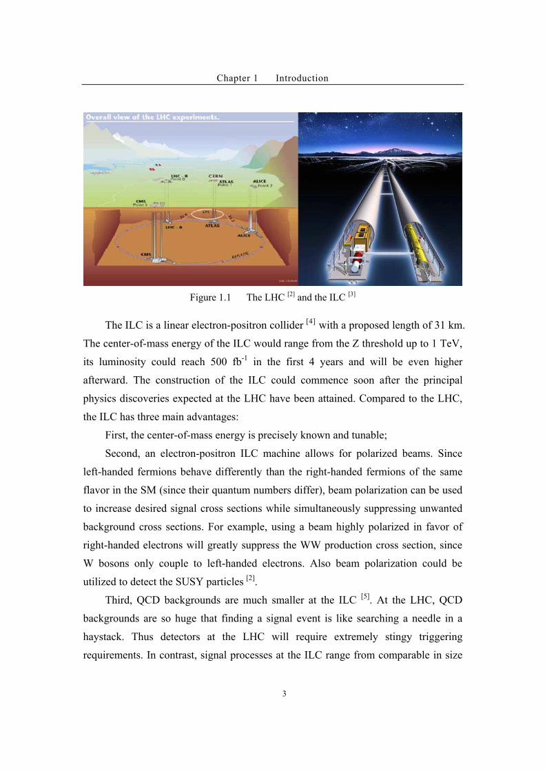
Figure 1.1 The LHC [2] and the ILC [3]
The ILC is a linear electron-positron collider [4]
with a proposed length of 31 km.
The center-of-mass energy of the ILC would range from the Z threshold up to 1 TeV,
its luminosity could reach 500 fb-1
in the first 4 years and will be even higher
afterward. The construction of the ILC could commence soon after the principal
physics discoveries expected at the LHC have been attained. Compared to the LHC,
the ILC has three main advantages:
First, the center-of-mass energy is precisely known and tunable;
Second, an electron-positron ILC machine allows for polarized beams. Since
left-handed fermions behave differently than the right-handed fermions of the same
flavor in the SM (since their quantum numbers differ), beam polarization can be used
to increase desired signal cross sections while simultaneously suppressing unwanted
background cross sections. For example, using a beam highly polarized in favor of
right-handed electrons will greatly suppress the WW production cross section, since
W bosons only couple to left-handed electrons. Also beam polarization could be
utilized to detect the SUSY particles [2]
.
Third, QCD backgrounds are much smaller at the ILC [5]
. At the LHC, QCD
backgrounds are so huge that finding a signal event is like searching a needle in a
haystack. Thus detectors at the LHC will require extremely stingy triggering
requirements. In contrast, signal processes at the ILC range from comparable in size
Chapter 1 Introduction
4
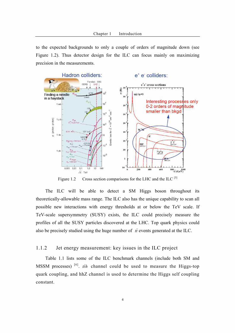
to the expected backgrounds to only a couple of orders of magnitude down (see
Figure 1.2). Thus detector design for the ILC can focus mainly on maximizing
precision in the measurements.
Figure 1.2 Cross section comparisons for the LHC and the ILC [5]
The ILC will be able to detect a SM Higgs boson throughout its
theoretically-allowable mass range. The ILC also has the unique capability to scan all
possible new interactions with energy thresholds at or below the TeV scale. If
TeV-scale supersymmetry (SUSY) exists, the ILC could precisely measure the
profiles of all the SUSY particles discovered at the LHC. Top quark physics could
also be precisely studied using the huge number of tt events generated at the ILC.
1.1.2 Jet energy measurement: key issues in the ILC project!
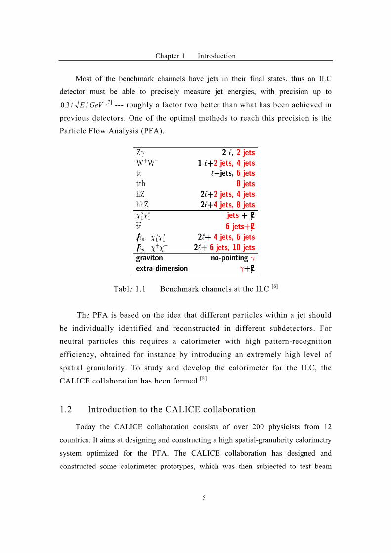
Table 1.1 lists some of the ILC benchmark channels (include both SM and
MSSM processes) [6]
. htt channel could be used to measure the Higgs-top
quark coupling, and hhZ channel is used to determine the Higgs self coupling
constant.
Chapter 1 Introduction
5
Most of the benchmark channels have jets in their final states, thus an ILC
detector must be able to precisely measure jet energies, with precision up to
GeVE //3.0[7]
--- roughly a factor two better than what has been achieved in
previous detectors. One of the optimal methods to reach this precision is the
Particle Flow Analysis (PFA).
Table 1.1 Benchmark channels at the ILC [6]
The PFA is based on the idea that different particles within a jet should
be individually identified and reconstructed in different subdetectors. For
neutral particles this requires a calorimeter with high pattern-recognition
efficiency, obtained for instance by introducing an extremely high level of
spatial granularity. To study and develop the calorimeter for the ILC, the
CALICE collaboration has been formed [8]
.
1.2 Introduction to the CALICE collaboration
Today the CALICE collaboration consists of over 200 physicists from 12
countries. It aims at designing and constructing a high spatial-granularity calorimetry
system optimized for the PFA. The CALICE collaboration has designed and
constructed some calorimeter prototypes, which was then subjected to test beam
Chapter 1 Introduction
6
experiments. Aims of these studies have been twofold:
To study the physics performances of highly granular calorimeters;
Check the feasibility of large detectors with “technological” prototypes;
Improve the MC simulation tools use the test beam data.
A large amount of test beam data has been obtained in the test beam program.
The analysis of said data is part of thesis (see Chapter 5 and Chapter 6).
1.3 Main contribution and outline of this thesis
This thesis is divided into seven chapters. Chapter 2 and Chapter 3 are dedicated
to the introduction of relevant backgrounds: in Chapter 2 we introduce the physics
backgrounds (Higgs physics at ILC) and in Chapter 3 we deal more specifically with
backgrounds in an ILC machine, detector and software. Higgs boson mass and
production cross section measurements are discussed in Chapter 4. After a discussion
on radiation effects and backgrounds, the model-independent and model-dependent
analyses are presented, and then Chapter 4 concludes with a preliminary study on
beam-parameter selection.
Chapter 5 and Chapter 6 are associated with the CALICE test beam data analysis.
In Chapter 5 we outline the experimental set up and present its data flow, calibration
and data-quality checks. Chapter 6 focuses on the energy, spatial and angular
resolutions of the CALICE ECAL prototype. Here we introduce a track-free
algorithm for angle measurements which could be used to measure the direction of an
injection photon with ECAL hits. In Chapter 7 we summarize our results and give a
brief perspective overview.
For the Higgs boson mass and cross section measurements, the
!!HHZee ""#$ channel acted as the signal, with all radiation effects and SM
backgrounds taken into account. The mass of the Higgs boson was assumed to be
120GeV, and the center-of-mass energy was set to 230GeV. The recoil mass method,
which requires no information concerning the Higgs decay final state, was used for
the mass measurement. This obviated the need for employing any potentially
model-dependent cuts, rendering this model independent analysis. The precision of
Chapter 1 Introduction
7
the resulting Higgs boson mass measurement was 38MeV. A cross section precision
of 5% was also obtained. Inclusion of some assumptions as to the Higgs decay final
state (such as limiting the analysis to a SM Higgs boson or an invisibly-decaying
Higgs boson) improved the mass-measurement precision to 29 MeV (and the cross
section measurement precision to 4%) – about a 25% improvement as compared to
the model independent analysis. A fast simulation tool that could predict the Higgs
boson recoil mass spectrum was also developed and utilized in a preliminary study on
beam-parameter optimization (see Chapter 4).
In the CALICE test beam data analysis, my work is focused on data-quality
checks and track-free ECAL angular resolution determinations.
We collected a large amount of data in the CALICE test beam experiments. The
quality of data directly affects the results from the analysis. We made a scan of almost
all the data files collected in the 2006-2007 CALICE test beam experiment, searching
for abnormal signals, unexpected phenomena (for example a bump in the total energy
spectrum, time-dependent noise, etc.) and quickly fed results back to the collaboration.
The data files have also been classified into different groups, making it easier for later
analyses (see Chapter 5).
The energy, spatial and angular resolutions are considered as the characteristic
parameters of a calorimeter. We have developed a track-free angular resolution
algorithm (using only the ECAL information), and have compared results from our
algorithm with previous CALICE collaboration angular-measurement results (which
use drift-chamber information to reconstruct a reference track). The motivation to
develop a track-free algorithm is to measure the injection direction of a photon which
might be generated beyond the interaction point (for example, a FSR photon or a
photon resulting from the decay of a long-lived neutral SUSY particle), see section
6.3.
Chapter 2 Higgs Physics at the ILC
8
Chapter 2 Higgs Physics at the ILC
2.1 Introduction: Higgs Particle in the SM and beyond
The origin of mass is one of the essential questions that particle physics attempts
to answer. In the SM (Standard Model), particles gain their mass through the
interactions with the Higgs field. The Higgs field is an isodoublet complex scalar
field which breaks the electroweak symmetry to the electromagnetic symmetry
(SU(2)L×U(1)Y ! U(1)EM) by acquiring an non-zero vacuum expectation value
through its self-interactions. Masses are generated for the gauge bosons of the weak
interaction (W±, Z) when they absorb three would-be Goldstone bosons, and the
fermions get their mass through Yukawa couplings with the Higgs field. The sole
remaining degree of freedom from the Higgs field forms the Higgs particle.
A Spontaneous Symmetry Breaking (SSB) mechanism, which necessitates the
existence a Higgs sector, is the way to generate mass in many physics models beyond
the SM, for example, the MSSM (Minimal Supersymmetric Standard Model) or the
Little Higgs models. Now let’s review the Higgs sectors in these two highly-popular
beyond-the-SM physics models [10]
.
In the MSSM, two Higgs isodoublets have eight degrees of freedom. After SSB,
three degrees of freedom have been absorbed and act as the longitudinal degrees of
freedom of the gauge bosons (W±, Z), and the remaining five degrees of freedom
remain as Higgs particles. So instead of the one neutral CP-even Higgs particle in the
SM, five Higgs particles in the MSSM: two charged Higgs particles (H±), two
CP-even Higgs particles (h and H; where h is the lighter Higgs particle) and one
CP-odd Higgs particle (A). The upper limit of the lightest Higgs (h) mass ranges from
~100GeV to ~140GeV, depending upon the choice of various input parameters, while
the masses of the other MSSM Higgs particles range from 240GeV to 1TeV.
In Little Higgs models, Higgs particles are viewed as Goldstone bosons
generated via a SSB process. As described by the Goldstone theorem, a Goldstone
Chapter 2 Higgs Physics at the ILC
9
boson always has zero mass, so the mass of the Higgs particles should be much lower
than the energy scale of the SSB process ---- which means there exist some new
SSB-associated interactions at an energy scale much higher than the TeV-scale.
These new interactions (perhaps SM-like) bring with them a family of new particles.
Up to now, the SM has had myriad success in explaining nearly all experimental
phenomena, but the predicted Higgs particle has not yet been discovered in the
laboratory. This Higgs particle is the only particle predicted by the SM which has not
yet been directly found. So searching for Higgs particle and precisely measuring its
properties is one of the central tasks for the LHC and ILC. In experimental particle
physics, the key problems about Higgs particle are:
Is there a Higgs particle? How can we detect it in the laboratory?
What is the nature of the Higgs particle? Is there any physics beyond the SM?
In this chapter we will introduce the SM Higgs boson and the measurements of
its properties at the ILC.
2.2 The SM Higgs Particle
The SM Higgs particle is a spin-parity 0+
particle, and its mass is the only
unknown parameter in the symmetry-breaking sector of the SM. There are
strong constraints on the Higgs boson mass: the lower limit on the SM
Higgs boson mass is 114GeV at 95% CL [11]
, given by the LEP experiments; if
the SM is valid up to scales near the Planck scale, the Higgs boson mass is
constraint to lay within the 130-190GeV range. If the mass of the Higgs
particle lies beyond this constraint, new interactions are expected to occur
between ~1TeV to the Planck scale: the heavier the Higgs particle is, the
lower the scale of new physics is. If the Higgs particle were to be as massive
as 1TeV, then we would expect to observe new interactions at the TeV scale.
(So the unique capability of ILC – fully scan for new interactions at the TeV
scale – is very attractive.)
In the SM, the masses of other particles are proportional to their
couplings to the Higgs particle, and the mass of Higgs particle constrains the
Chapter 2 Higgs Physics at the ILC
10
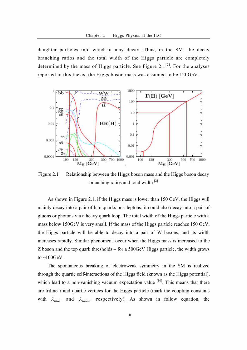
daughter particles into which it may decay. Thus, in the SM, the decay
branching ratios and the total width of the Higgs particle are completely
determined by the mass of Higgs particle. See Figure 2.1[2]
. For the analyses
reported in this thesis, the Higgs boson mass was assumed to be 120GeV.
Figure 2.1 Relationship between the Higgs boson mass and the Higgs boson decay
branching ratios and total width [2]
As shown in Figure 2.1, if the Higgs mass is lower than 150 GeV, the Higgs will
mainly decay into a pair of b, c quarks or $ leptons; it could also decay into a pair of
gluons or photons via a heavy quark loop. The total width of the Higgs particle with a
mass below 150GeV is very small. If the mass of the Higgs particle reaches 150 GeV,
the Higgs particle will be able to decay into a pair of W bosons, and its width
increases rapidly. Similar phenomena occur when the Higgs mass is increased to the
Z boson and the top quark thresholds – for a 500GeV Higgs particle, the width grows
to ~100GeV.
The spontaneous breaking of electroweak symmetry in the SM is realized
through the quartic self-interactions of the Higgs field (known as the Higgs potential),
which lead to a non-vanishing vacuum expectation value [10]
. This means that there
are trilinear and quartic vertices for the Higgs particle (mark the coupling constants
with HHH% and HHHH% respectively). As shown in follow equation, the
Chapter 2 Higgs Physics at the ILC
11
corresponding couplings are proportional to the square of Higgs boson mass. Direct
measurement to the Higgs boson self-coupling ( HHH% ) would be the most decisive
experimental confirmation of the SM framework
422 5.0)( &%&!& $#'V
223 HFHHH MG'% "223 HFHHHH MG'% .
Next let’s introduce the measurements of Higgs particle properties at the ILC.
2.3 Measurement of the SM Higgs particle mass at the ILC
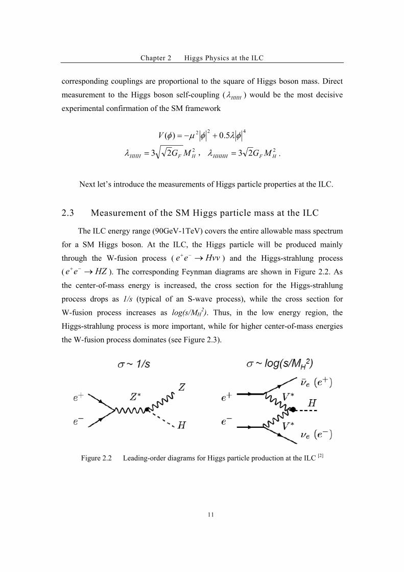
The ILC energy range (90GeV-1TeV) covers the entire allowable mass spectrum
for a SM Higgs boson. At the ILC, the Higgs particle will be produced mainly
through the W-fusion process ( Hvvee "#$) and the Higgs-strahlung process
( HZee "#$). The corresponding Feynman diagrams are shown in Figure 2.2. As
the center-of-mass energy is increased, the cross section for the Higgs-strahlung
process drops as 1/s (typical of an S-wave process), while the cross section for
W-fusion process increases as log(s/MH2). Thus, in the low energy region, the
Higgs-strahlung process is more important, while for higher center-of-mass energies
the W-fusion process dominates (see Figure 2.3).
Figure 2.2 Leading-order diagrams for Higgs particle production at the ILC [2]
Chapter 2 Higgs Physics at the ILC
12
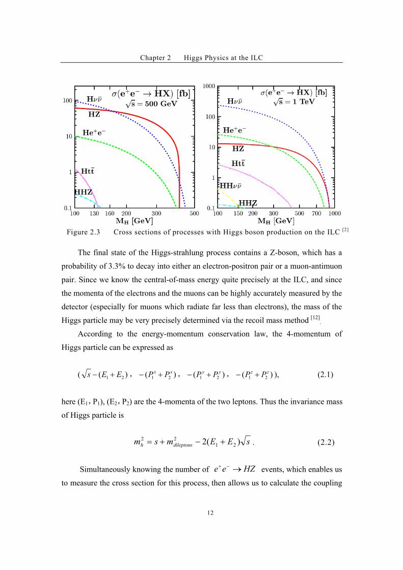
Figure 2.3 Cross sections of processes with Higgs boson production on the ILC [2]
The final state of the Higgs-strahlung process contains a Z-boson, which has a
probability of 3.3% to decay into either an electron-positron pair or a muon-antimuon
pair. Since we know the central-of-mass energy quite precisely at the ILC, and since
the momenta of the electrons and the muons can be highly accurately measured by the
detector (especially for muons which radiate far less than electrons), the mass of the
Higgs particle may be very precisely determined via the recoil mass method [12]
.
According to the energy-momentum conservation law, the 4-momentum of
Higgs particle can be expressed as
( )( 21 EEs $# " )( 21
xx PP $# " )( 21
yy PP $# " )( 21
zz PP $# ), (2.1)
here (E1"P1), (E2"P2) are the 4-momenta of the two leptons. Thus the invariance mass
of Higgs particle is
sEEmsm dileptonsh )(2 21
22 $#$' . (2.2)
Simultaneously knowing the number of HZee "#$ events, which enables us
to measure the cross section for this process, then allows us to calculate the coupling
Chapter 2 Higgs Physics at the ILC
13
between the Higgs particle and the Z boson: () LNg /2 '* .
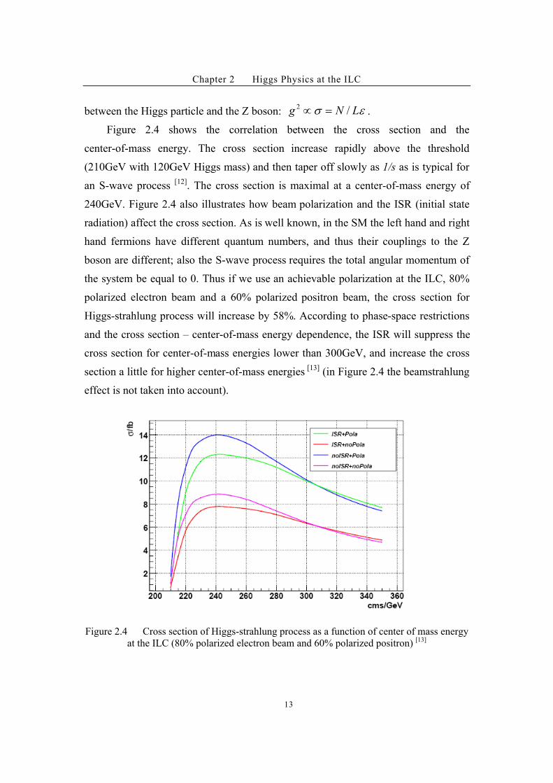
Figure 2.4 shows the correlation between the cross section and the
center-of-mass energy. The cross section increase rapidly above the threshold
(210GeV with 120GeV Higgs mass) and then taper off slowly as 1/s as is typical for
an S-wave process [12]
. The cross section is maximal at a center-of-mass energy of
240GeV. Figure 2.4 also illustrates how beam polarization and the ISR (initial state
radiation) affect the cross section. As is well known, in the SM the left hand and right
hand fermions have different quantum numbers, and thus their couplings to the Z
boson are different; also the S-wave process requires the total angular momentum of
the system be equal to 0. Thus if we use an achievable polarization at the ILC, 80%
polarized electron beam and a 60% polarized positron beam, the cross section for
Higgs-strahlung process will increase by 58%. According to phase-space restrictions
and the cross section – center-of-mass energy dependence, the ISR will suppress the
cross section for center-of-mass energies lower than 300GeV, and increase the cross
section a little for higher center-of-mass energies [13]
(in Figure 2.4 the beamstrahlung
effect is not taken into account).
Figure 2.4 Cross section of Higgs-strahlung process as a function of center of mass energy
at the ILC (80% polarized electron beam and 60% polarized positron) [13]

Chapter 2 Higgs Physics at the ILC
14
The momentum of a charged particle is measured through the bending of its
track in the magnetic field of the detector. This means that lower energy tracks yield
better track momentum resolution, so that using a smaller center-of-mass energy
would result in a gain in the Higgs boson mass resolution. In this thesis, with
assuming a 120GeV Higgs boson mass, we set the center-of-mass energy equal to
230GeV, which is slightly less than the energy at which the cross-section reaches its
maximum value. With an integrated luminosity of 500fb-1
, the Higgs boson mass can
be measured to a precision of 38 MeV (model independent analysis) or 29 MeV
(model dependent analysis) see Chapter 4.
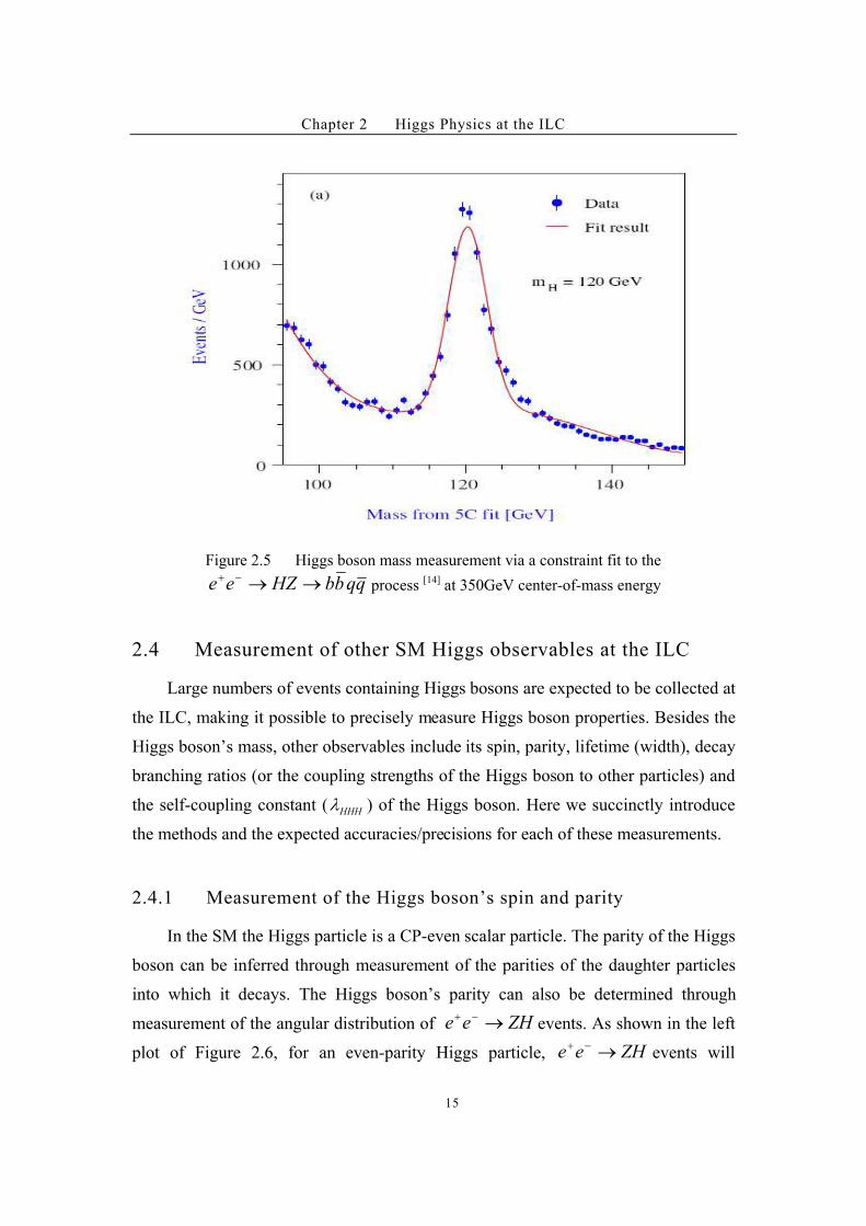
Besides the recoil mass method, the Higgs boson mass could also be measured
via a constraint fit method with the qqbbHZee ""#$ process – by measuring
directly the jet momenta from the Higgs boson decay [14]
. The Higgs boson mass
determination relies on a kinematical 5-C fit imposing energy and momentum
conservation and requiring the mass of the jet pair closest to the Z mass correspond to
Mz. The main advantage of this constraint fit method is the large statistics available
with this process. And, since the relative error on the Higgs boson mass measurement
is proportional to the relative error on the jet energy resolution, this method yields
better results as the center-of-mass energy is increased. Given a 350GeV
center-of-mass energy and 500fb-1
of integrated luminosity, the precision of the Higgs
boson mass measurement is 70 MeV. Results from such a fit are shown in Figure 2.5.
Chapter 2 Higgs Physics at the ILC
15
Figure 2.5 Higgs boson mass measurement via a constraint fit to the
qqbbHZee ""#$process [14] at 350GeV center-of-mass energy
2.4 Measurement of other SM Higgs observables at the ILC
Large numbers of events containing Higgs bosons are expected to be collected at
the ILC, making it possible to precisely measure Higgs boson properties. Besides the
Higgs boson’s mass, other observables include its spin, parity, lifetime (width), decay
branching ratios (or the coupling strengths of the Higgs boson to other particles) and
the self-coupling constant ( HHH% ) of the Higgs boson. Here we succinctly introduce
the methods and the expected accuracies/precisions for each of these measurements.
2.4.1 Measurement of the Higgs boson’s spin and parity
In the SM the Higgs particle is a CP-even scalar particle. The parity of the Higgs
boson can be inferred through measurement of the parities of the daughter particles
into which it decays. The Higgs boson’s parity can also be determined through
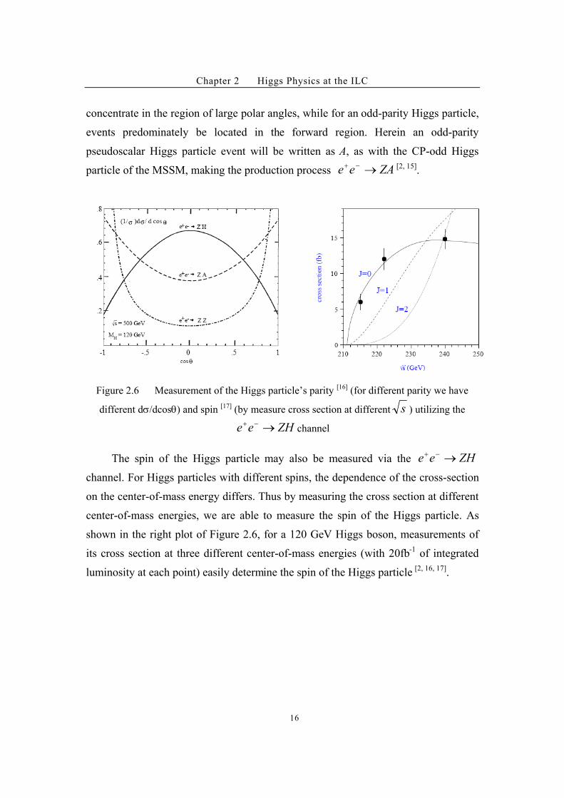
measurement of the angular distribution of ZHee "#$events. As shown in the left
plot of Figure 2.6, for an even-parity Higgs particle, ZHee "#$events will
Chapter 2 Higgs Physics at the ILC
16
concentrate in the region of large polar angles, while for an odd-parity Higgs particle,
events predominately be located in the forward region. Herein an odd-parity
pseudoscalar Higgs particle event will be written as A, as with the CP-odd Higgs
particle of the MSSM, making the production process ZAee "#$ [2, 15].
Figure 2.6 Measurement of the Higgs particle’s parity [16] (for different parity we have
different d)/dcos+) and spin [17] (by measure cross section at different s ) utilizing the
ZHee "#$channel
The spin of the Higgs particle may also be measured via the ZHee "#$
channel. For Higgs particles with different spins, the dependence of the cross-section
on the center-of-mass energy differs. Thus by measuring the cross section at different
center-of-mass energies, we are able to measure the spin of the Higgs particle. As
shown in the right plot of Figure 2.6, for a 120 GeV Higgs boson, measurements of
its cross section at three different center-of-mass energies (with 20fb-1
of integrated
luminosity at each point) easily determine the spin of the Higgs particle [2, 16, 17]
.
Chapter 2 Higgs Physics at the ILC
17
2.4.2 Measurements of the decay branching ratios and total width
Measurements of Higgs boson decay branching ratios (equivalent to determining
the coupling constants of other particles to the Higgs boson) are very important; these
can be used to check the validity of the SM and to explore the nature of the Higgs
particle. For example, by comparing the coupling constants of a Higgs particle to the
positively-charged quarks (u, c, t) and the negatively charged quarks (d, s, b), we can
check whether an observed Higgs boson is consistent with a SM Higgs boson or, if
not, with one of the Higgs bosons expected within SUSY scenarios.
The measurements of the coupling constants between the Higgs boson and the
W, Z gauge bosons are straight-forward. These may be determined by measuring the
cross sections of the W-fusion and Higgs-strahlung processes. The precision of the
coupling constants measurements could reach 1%-2% level [2]
.
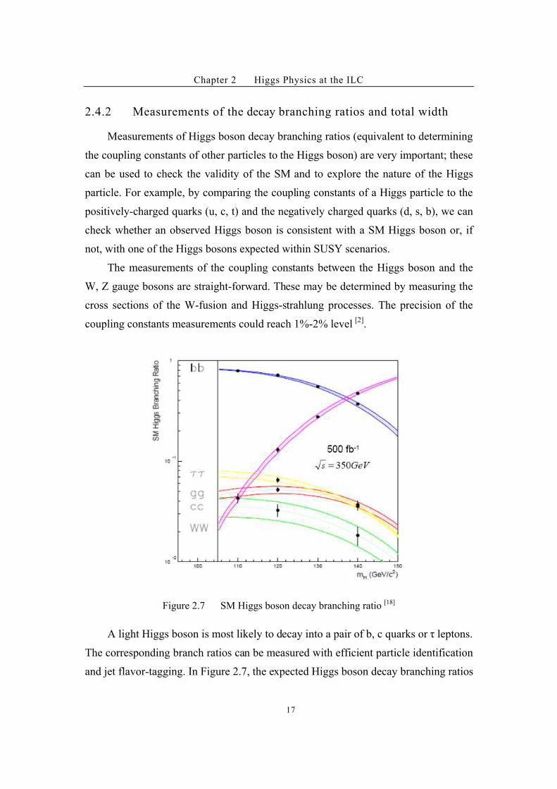
Figure 2.7 SM Higgs boson decay branching ratio [18]
A light Higgs boson is most likely to decay into a pair of b, c quarks or $ leptons.
The corresponding branch ratios can be measured with efficient particle identification
and jet flavor-tagging. In Figure 2.7, the expected Higgs boson decay branching ratios
Chapter 2 Higgs Physics at the ILC
18
are shown as functions of the Higgs boson’s mass. The widths of the color-coded
curve for each decay channel indicate the expected precision of the measurements [18]
.
Since the top quark is massive, the coupling constant of the Higgs particle to the
top quark is the largest of all the Higgs-fermion couplings in the SM. If the Higgs
particle is heavier than 350GeV, it is allowed to decay into a pair of top quarks, and
then we could directly measure the coupling constant. For example, if the Higgs
particle has a mass equal to 400GeV, assuming a center-of-mass energy of 800 GeV
and an integrated luminosity of 1ab-1
, then the coupling between the Higgs particle
and the top quark could be measured to a relative precision of 4%[19]
.
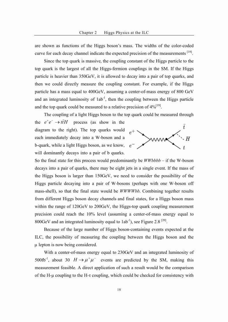
The coupling of a light Higgs boson to the top quark could be measured through
the Httee "#$ process (as show in the
diagram to the right). The top quarks would
each immediately decay into a W-boson and a
b-quark, while a light Higgs boson, as we know,
will dominantly decays into a pair of b quarks.
So the final state for this process would predominantly be WWbbbb – if the W-boson
decays into a pair of quarks, there may be eight jets in a single event. If the mass of
the Higgs boson is larger than 150GeV, we need to consider the possibility of the
Higgs particle decaying into a pair of W-bosons (perhaps with one W-boson off
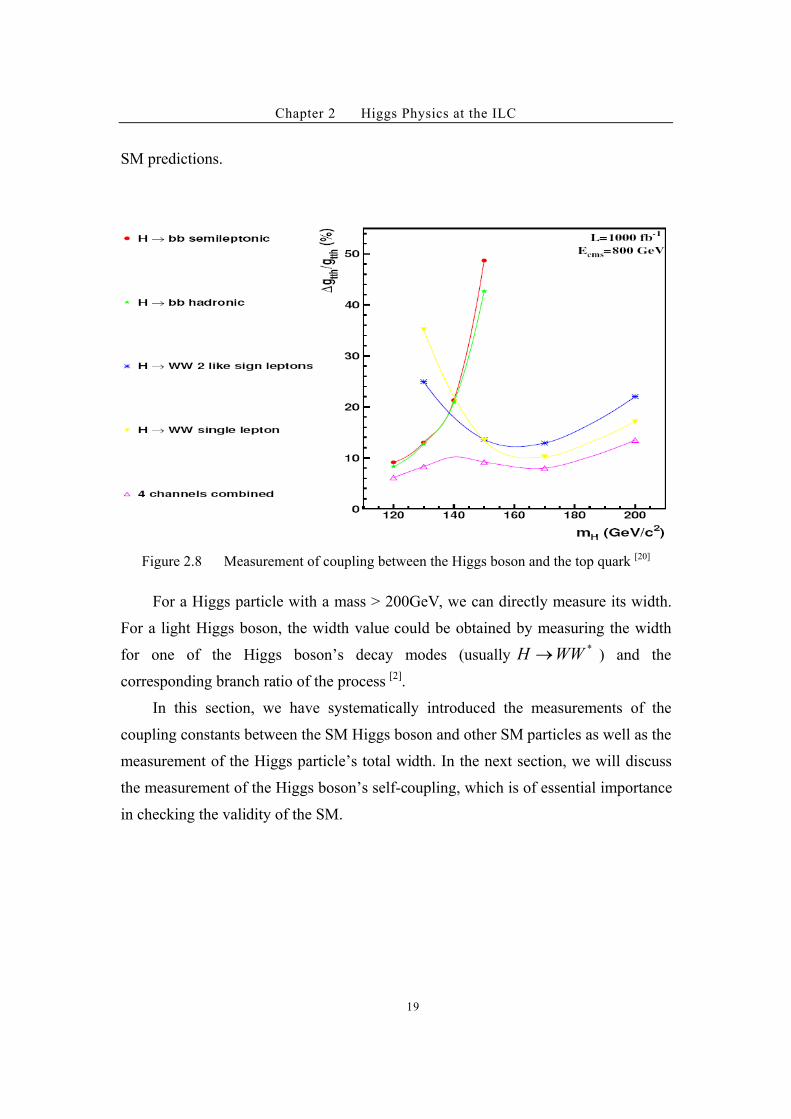
mass-shell), so that the final state would be WWWWbb. Combining together results
from different Higgs boson decay channels and final states, for a Higgs boson mass
within the range of 120GeV to 200GeV, the Higgs-top quark coupling measurement
precision could reach the 10% level (assuming a center-of-mass energy equal to
800GeV and an integrated luminosity equal to 1ab-1
), see Figure 2.8 [20]
.
Because of the large number of Higgs boson-containing events expected at the
ILC, the possibility of measuring the coupling between the Higgs boson and the
!,lepton is now being considered.
With a center-of-mass energy equal to 230GeV and an integrated luminosity of
500fb-1
, about 30 #$" !!H events are predicted by the SM, making this
measurement feasible. A direct application of such a result would be the comparison
of the H-# coupling to the H-$ coupling, which could be checked for consistency with
Chapter 2 Higgs Physics at the ILC
19
SM predictions.
Figure 2.8 Measurement of coupling between the Higgs boson and the top quark [20]
For a Higgs particle with a mass > 200GeV, we can directly measure its width.
For a light Higgs boson, the width value could be obtained by measuring the width
for one of the Higgs boson’s decay modes (usually*WWH " ) and the
corresponding branch ratio of the process [2]
.
In this section, we have systematically introduced the measurements of the
coupling constants between the SM Higgs boson and other SM particles as well as the
measurement of the Higgs particle’s total width. In the next section, we will discuss
the measurement of the Higgs boson’s self-coupling, which is of essential importance
in checking the validity of the SM.
Chapter 2 Higgs Physics at the ILC
20
2.4.3 Measurement of the Higgs boson’s self-coupling
The measurement of the trilinear Higgs boson self-coupling ( HHH% ) constant
will be the first non-trivial probe of the Higgs potential and probably the most
decisive test of the Electroweak Symmetry Breaking (EWSB) mechanism[2]
. This
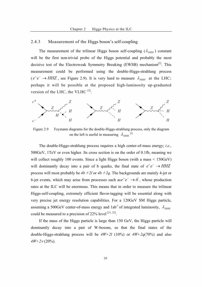
measurement could be performed using the double-Higgs-strahlung process
( HHZee "#$, see Figure 2.9). It is very hard to measure HHH% at the LHC;
perhaps it will be possible at the proposed high-luminosity up-graduated
version of the LHC, the VLHC [2]
.
Figure 2.9 Feymann diagrams for the double-Higgs-strahlung process, only the diagram
on the left is useful in measuring HHH% [2]
The double-Higgs-strahlung process requires a high center-of-mass energy; i.e.,
500GeV, 1TeV or even higher. Its cross section is on the order of 0.1fb, meaning we
will collect roughly 100 events. Since a light Higgs boson (with a mass < 150GeV)
will dominantly decay into a pair of b quarks, the final state of HHZee "#$
process will most probably be 4b!2l or 4b!2q. The backgrounds are mainly 4-jet or
6-jet events, which may arise from processes such as ttee "#$, whose production
rates at the ILC will be enormous. This means that in order to measure the trilinear
Higgs-self-coupling, extremely efficient flavor-tagging will be essential along with
very precise jet energy resolution capabilities. For a 120GeV SM Higgs particle,
assuming a 500GeV center-of-mass energy and 1ab-1
of integrated luminosity, HHH%
could be measured to a precision of 22% level [21, 22]
.
If the mass of the Higgs particle is large than 150 GeV, the Higgs particle will
dominantly decay into a pair of W-bosons, so that the final states of the
double-Higgs-strahlung process will be 4W+2l (10%) or 4W+2q(70%) and also
4W+2- (20%).
Chapter 2 Higgs Physics at the ILC
21
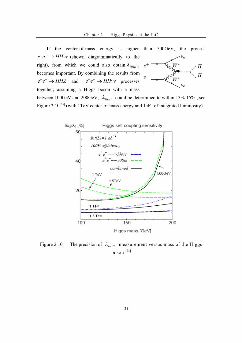
If the center-of-mass energy is higher than 500GeV, the process
HHvvee "#$(shown diagrammatically to the
right), from which we could also obtain HHH% ,
becomes important. By combining the results from
HHZee "#$and HHvvee "#$
processes
together, assuming a Higgs boson with a mass
between 100GeV and 200GeV, HHH% could be determined to within 13%-15% , see
Figure 2.10[23]
(with 1TeV center-of-mass energy and 1ab-1
of integrated luminosity).
Figure 2.10 The precision of HHH% measurement versus mass of the Higgs
boson [23]
Chapter 2 Higgs Physics at the ILC
22
2.5 Summary
In this chapter we have briefly introduced the Higgs physics at the ILC; i.e.,
measurements of properties of the SM Higgs boson. These parameters include its
mass, lifetime, spin, parity, couplings to other SM particles and the trilinear Higgs
boson self-coupling ( HHH% ).
We have examined two methods useful in determining the Higgs boson mass at
the ILC: the recoil mass method utilizing the !!HHZee ""#$channel and the
constraint fit method employed for hadronic final states of the HZee "#$process.
The former performs better at low center-of-mass energies while the latter becomes
important for higher center-of-mass energies. Assuming the mass of the Higgs
boson to be 120GeV, and for a 230GeV center-of-mass energy with 500fb-1
of
integrated luminosity, the first method enables the Higgs boson mass to be
measured to a precision of 30-40 MeV. On the other hand, if the
center-of-mass energy is 350 GeV, then the second method would allow us to
achieve a mass measurement precision of 70 MeV.
The parity of the Higgs particle could be determined by studying the
angular distribution of HZee "#$events. By measuring the cross section of
the HZee "#$process at different center-of-mass energies, we could
ascertain the spin of the Higgs particle. In the SM, the width (lifetime) of the
Higgs particle is determined by its mass. If the mass is larger than 150 GeV,
then the Higgs boson’s width is wide enough to be measured directly; on the
other hand, if the mass is smaller than 150 GeV, its total width could be
calculated from the measurements of the partial width of one decay mode
(usually*WWH " ) and the corresponding branching ratio.
In the SM, the coupling of any other particle to the Higgs boson is
proportional to the mass of the particle. Since the leading processes for Higgs
particle production at the ILC are HZee "#$and Hvvee "#$
, the
couplings of the Higgs boson to the Z, W bosons could be directly determined
from respective measurements of these two processes, for which we should be
able to easily reach precisions at the 1%-2% level. A light Higgs boson will
mainly decay into a pair of b, c quarks or $ leptons, so the couplings of these

Chapter 2 Higgs Physics at the ILC
23
three fermion flavors to the Higgs boson can be determined with the support
of effective jet flavor-tagging and particle identification, and the measured
precisions could reach the 2%-10% level.
The situation concerning the measurement of the coupling of the Higgs
particle to the top quark is a little more complex. Since the top quark has a
huge mass, the Higgs particle needs to be at least as massive as 350 GeV to
decay directly into a pair of top quarks, which would allow for a direct
measurement of the top-Higgs coupling. Otherwise, if the Higgs boson is too
light, we can determine the coupling via the Httee "#$process – with a
center-of-mass energy equal to 800GeV and an integrated luminosity of 1ab-1
,
the precision for determining the top-Higgs coupling via this channel could
reach the 10% level for a Higgs boson with a mass between 120GeV and
200GeV.
Determining the value of the trilinear Higgs boson self-coupling is one of
the most exciting challenges in the ILC physics. A measured value for this
coupling will probably be the first non-trivial probe of the Higgs potential as
well as the most decisive test of EWSB. With an integrated luminosity of
1ab-1
and a center-of-mass energy of 500GeV (1TeV), precision for the
determination of the trilinear Higgs boson self-coupling could reach the 22%
(15%) level using the double-Higgs-strahlung process (both HHZee "#$and
HHvvee "#$processes).
As we have discussed in this chapter, the ILC will have the capability to
provide precise measurements for almost all SM Higgs boson properties if the
Higgs boson’s mass is below 1TeV. The ILC should also present a decisive
test for the SM (and the EWSB mechanism). In Chapter 4, we will continue
our discussion on the Higgs boson mass and cross section measurements via
the !!HHZee ""#$channel.
Chapter 3 Introduction to the ILC accelerator, detector and software
24
Chapter 3 Introduction to the ILC accelerator,
detector and software
3.1 Introduction
As the next generation of linear collider, the ILC project is a great challenge to
the current technique on accelerator and detector. As for the accelerator, it is required
that [24]
:
Continuously tunable center-of-mass energy from 200GeV to 500GeV, with the
capability to be upgraded to 1TeV;
High luminosity with peak value as high as 2#1034
cm-2
s-1
, reaching an
integrated luminosity of 500fb-1
in the first four years;
Polarized beam; more than 80% electron polarization and more than 60%
positron polarization at the Interaction Point (IP);
An energy stability and precision of 0.1% level;
Capabilities of electron-electron and photon-photon collisions.
For the detector, it needs to have the capability of effectively identify the basic
quanta (quark, lepton and Mediate Gauge bosons) and precisely measure their
4-momentum [25]
. In other words, for the detector it requires:
Precise jet energy resolution;
Effective jet flavor tagging;
Very high precision on charged track momentum measurement (e, #, %);
Full solid angle coverage.
In this chapter we give a brief introduction to the ILC accelerator, detector and
its software system. Chapter 3.2 is the introduction to the current four ILC detector
concepts, chapter 3.3 will mainly present the emergence of International Large
Detector (ILD) group and the corresponding progress and organization on the
Chapter 3 Introduction to the ILC accelerator, detector and software
25
detector optimization study. Chapter 3.4 focuses on the detector model utilized in our
full simulation study (LDC01_Sc) and gives corresponding parameters. Chapter 3.5
outlines the ILC accelerator and the beam-beam effect, and in chapter 3.6 we briefly
present our software system, and it use the grid technique in the CALICE experiment.
A short summary comes in chapter 3.7.
3.2 Current four ILC detector concepts
Four ILC detector concepts emerged from preliminary detector studies, the SiD,
LDC, GLD and 4th
[25]
. In order to meet the requirement we mentioned in the
introduction, these four concepts shares many patterns in common. For example:
. Full and hermetic solid angle coverage;
. Vertex detector supported with the silicon-strips pixels technique, providing
the capability of precisely measure charged track and reconstruct the vertex –
excellent heavy quark identification;
. Highly efficient tracking, aiming a charged particle momentum resolution of
152 /105/ ##/0 GeVPP1 ;
. High magnetic field, with field strength from 3 Tesla to 5 Tesla;
. Putting the calorimetry system inside of the magnetic coil to ensure high
precision jet energy measurement. For all the four concepts, the di-jet mass
resolution could reach 3% level.
Of course, as four independent detector concepts, they also have many different
patterns. Now we start to introduce them one by one.
3.2.1 The SiD concept
The SiD concept, as well as the LDC and GLD concepts, adopts the
particle flow calorimeter, where highly segmented electromagnetic
calorimeter (ECAL) and hadron calorimeter (HCAL) allow the separation and
identification of energy deposition from different sources (charged track,
photons and neutral hadrons).
For the SiD concept, highly pixilized silicon-tungsten ECAL and
Chapter 3 Introduction to the ILC accelerator, detector and software
26
multi-layered, highly segmented hadron calorimeter have been adopted. Since
the calorimetry system is very expensive, the SiD concept utilizes the highest
field solenoid (5 Tesla) of all the four concepts to reduce the cost. The SiD
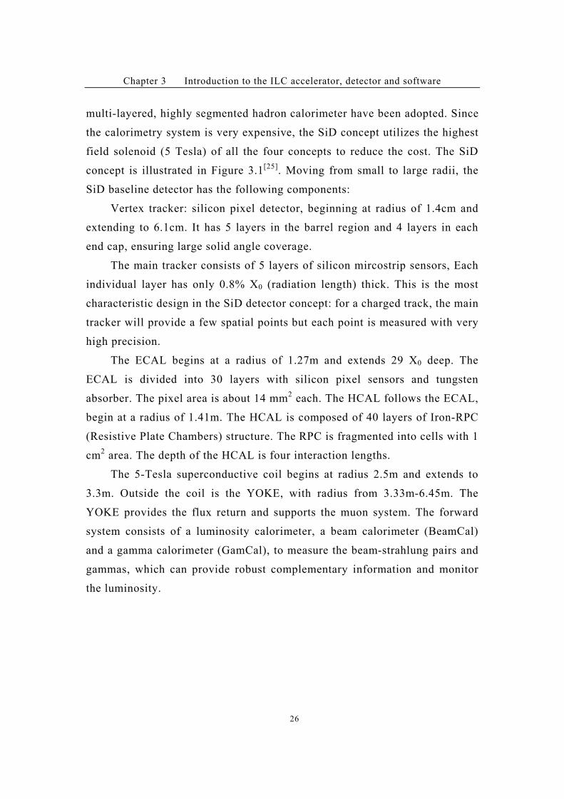
concept is illustrated in Figure 3.1[25]
. Moving from small to large radii, the
SiD baseline detector has the following components:
Vertex tracker: silicon pixel detector, beginning at radius of 1.4cm and
extending to 6.1cm. It has 5 layers in the barrel region and 4 layers in each
end cap, ensuring large solid angle coverage.
The main tracker consists of 5 layers of silicon mircostrip sensors, Each
individual layer has only 0.8% X0 (radiation length) thick. This is the most
characteristic design in the SiD detector concept: for a charged track, the main
tracker will provide a few spatial points but each point is measured with very
high precision.
The ECAL begins at a radius of 1.27m and extends 29 X0 deep. The
ECAL is divided into 30 layers with silicon pixel sensors and tungsten
absorber. The pixel area is about 14 mm2 each. The HCAL follows the ECAL,
begin at a radius of 1.41m. The HCAL is composed of 40 layers of Iron-RPC
(Resistive Plate Chambers) structure. The RPC is fragmented into cells with 1
cm2 area. The depth of the HCAL is four interaction lengths.
The 5-Tesla superconductive coil begins at radius 2.5m and extends to
3.3m. Outside the coil is the YOKE, with radius from 3.33m-6.45m. The
YOKE provides the flux return and supports the muon system. The forward
system consists of a luminosity calorimeter, a beam calorimeter (BeamCal)
and a gamma calorimeter (GamCal), to measure the beam-strahlung pairs and
gammas, which can provide robust complementary information and monitor
the luminosity.
Chapter 3 Introduction to the ILC accelerator, detector and software
27
Figure 3.1 Illustration of a quadrant of the SiD concept[25]
3.2.2 The LDC concept
The LDC concept takes a very high precision and robust tracking system
and a particle flow strategy based calorimetry system. The LDC concept
utilizes a large volume of tracking chamber with 4 Tesla field strength and
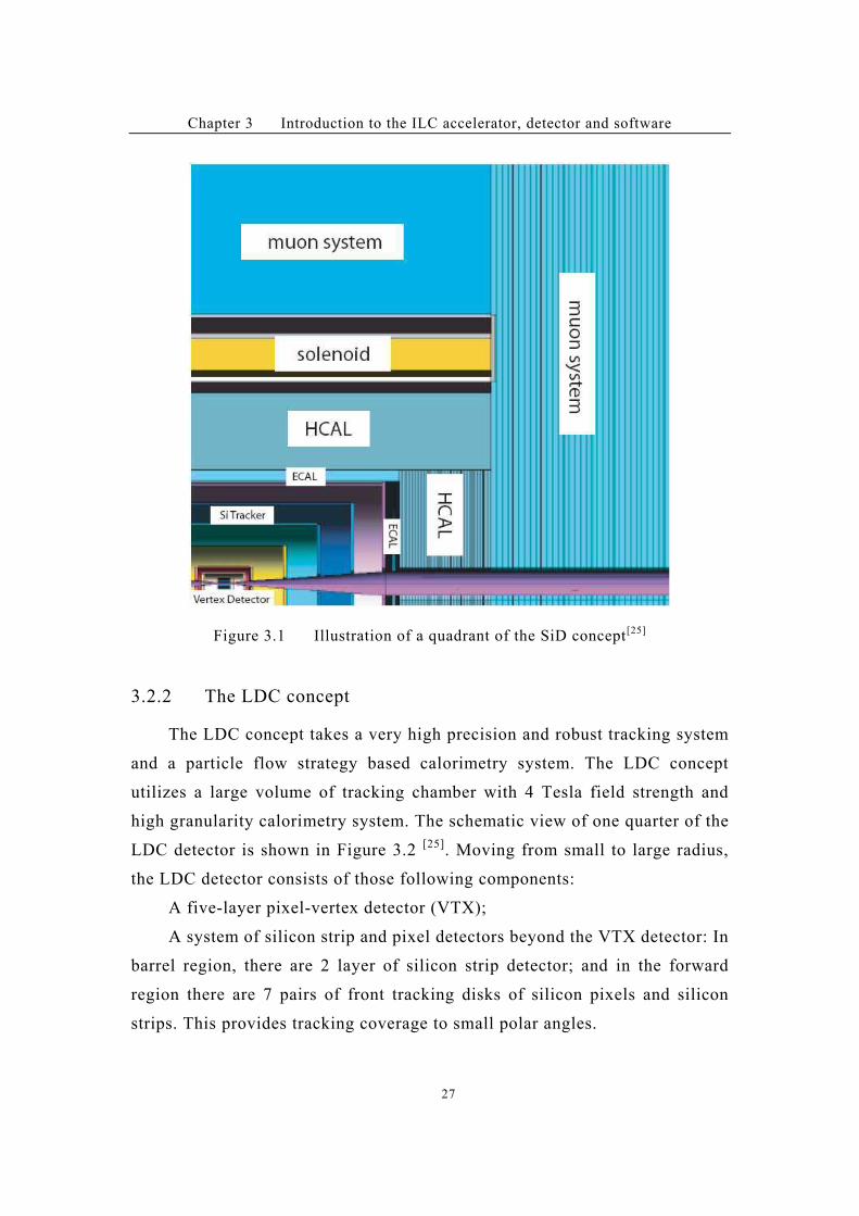
high granularity calorimetry system. The schematic view of one quarter of the
LDC detector is shown in Figure 3.2 [25]
. Moving from small to large radius,
the LDC detector consists of those following components:
A five-layer pixel-vertex detector (VTX);
A system of silicon strip and pixel detectors beyond the VTX detector: In
barrel region, there are 2 layer of silicon strip detector; and in the forward
region there are 7 pairs of front tracking disks of silicon pixels and silicon
strips. This provides tracking coverage to small polar angles.
Chapter 3 Introduction to the ILC accelerator, detector and software
28
The main tracker is a large volume of Time Projection Chamber (TPC),
which provides as many as 200 precisely measured spatial points for a high
energy charged track.
Figure 3.2 Schematic view of a quarter of the LDC detector [25]
In between the TPC and the ECAL, there exists a system of “linking”
detector based on silicon strip technique. There is Silicon External Tracker
(SET) in the barrel region and External Tracking Disk (ETD) in the endcap
region. The SET and ETD are only available for some recent versions of the
LDC concepts. In the concept utilized in our full simulation study, the
LDC01_Sc has no SET or ETD subdetectors.
The ECAL consists of 30 layers of silicon (sensor) and tungsten
Chapter 3 Introduction to the ILC accelerator, detector and software
29
(absorber) structure. The ECAL has very high spatial granularity: the silicon
sensor is segmented into 0.55cm#0.55cm cells on each layer (or 1cm#1cm
cells in some early versions). The front ending chips are installed into the
silicon sensor to save the space.
The HCAL consists of 40 layers of Iron-scintillator (or Iron-RPC)
sandwich structure. The HCAL also has high spatial granularity, while the
inner layer sensors are divided into 3cm#3cm cells (and 6cm#6cm or 12cm
# 12cm for outer layers). This design is so called the Analog HCAL
(AHCAL). There also exists another design of the HCAL sensor with
extremely high spatial granularity: utilizing 1/1cm2 cells, while for each
electronic channel we use only one bit to record the information if this cell is
hit or not. This design is called the Digital HCAL (DHCAL).
Outside the HCAL is the superconducting coil, which creates a 4-Tesla
longitudinal B-field. The flux return system is also the YOKE, which acts as
muon detector by interspersing some tracking detectors among the iron plates
(for some early version, there is no muon detector in the YOKE).
In the forward region there also has a system of extremely radiation
resistance calorimeters, to measure luminosity and to monitor the quality of
the collision. This system consists of LumiCal, BCAL and LHCAL.
The LDC concept has integrated into ILD concept. See section 3.3.
3.2.3 The GLD concept
The GLD concept [25]
has many things in common with LDC concept.
Both concepts choose TPC as the main tracking system, both utilize high
spatial granularity calorimetry system, which is optimized for the Particle
Flow Algorithm (PFA).
In the GLD concept, the field strength is 3 Tesla, which is the smallest of
the four concepts, at the meantime, it has the largest volume. The structure of
GLD concept is illustrated in Figure 3.3.
Chapter 3 Introduction to the ILC accelerator, detector and software
30
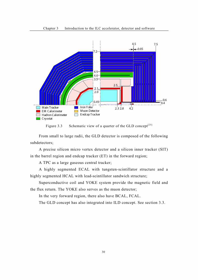
Figure 3.3 Schematic view of a quarter of the GLD concept[25]
From small to large radii, the GLD detector is composed of the following
subdetectors;
A precise silicon micro vertex detector and a silicon inner tracker (SIT)
in the barrel region and endcap tracker (ET) in the forward region;
A TPC as a large gaseous central tracker;
A highly segmented ECAL with tungsten-scintillator structure and a
highly segmented HCAL with lead-scintillator sandwich structure;
Superconductive coil and YOKE system provide the magnetic field and
the flux return. The YOKE also serves as the muon detector;
In the very forward region, there also have BCAL, FCAL.
The GLD concept has also integrated into ILD concept. See section 3.3.
Chapter 3 Introduction to the ILC accelerator, detector and software
31
3.2.4 The 4th
concept
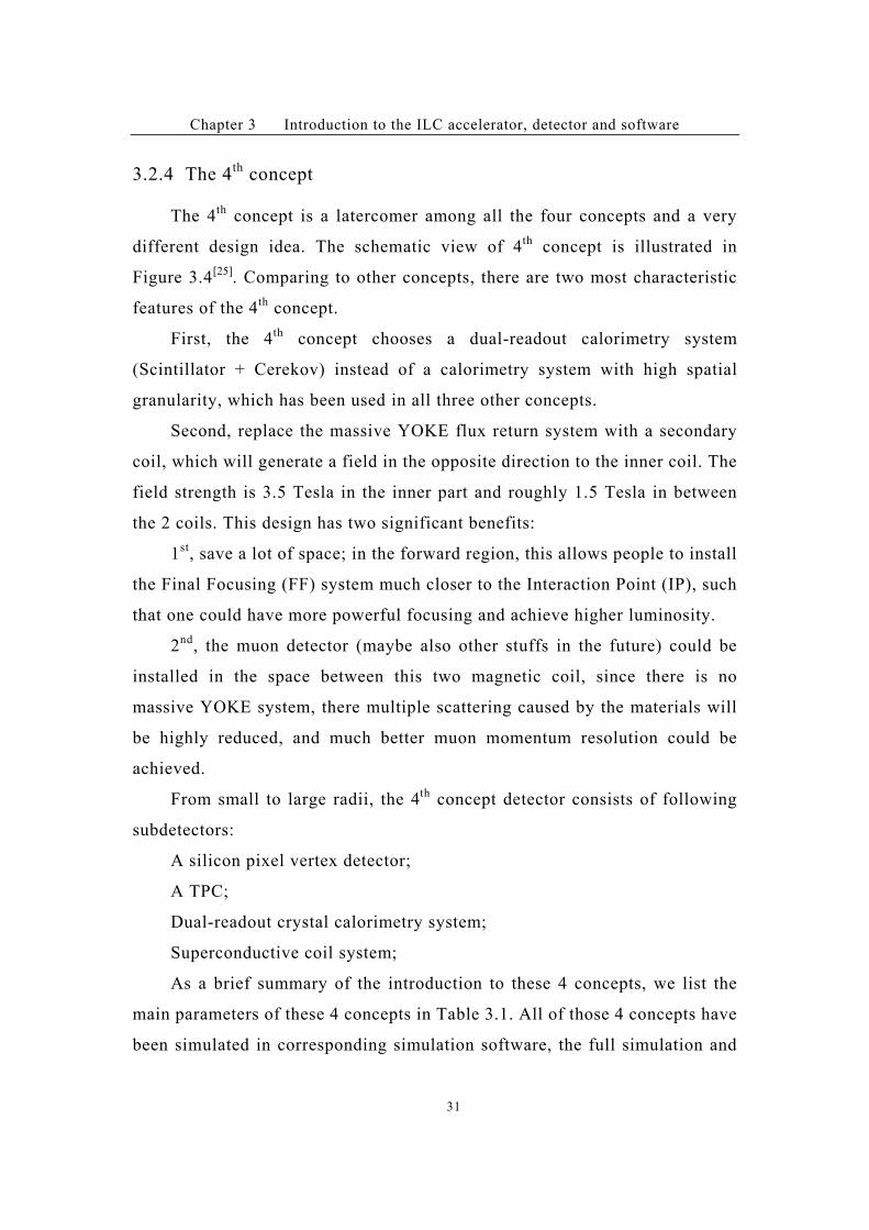
The 4th
concept is a latercomer among all the four concepts and a very
different design idea. The schematic view of 4th
concept is illustrated in
Figure 3.4[25]
. Comparing to other concepts, there are two most characteristic
features of the 4th
concept.
First, the 4th
concept chooses a dual-readout calorimetry system
(Scintillator + Cerekov) instead of a calorimetry system with high spatial
granularity, which has been used in all three other concepts.
Second, replace the massive YOKE flux return system with a secondary
coil, which will generate a field in the opposite direction to the inner coil. The
field strength is 3.5 Tesla in the inner part and roughly 1.5 Tesla in between
the 2 coils. This design has two significant benefits:
1st
, save a lot of space; in the forward region, this allows people to install
the Final Focusing (FF) system much closer to the Interaction Point (IP), such
that one could have more powerful focusing and achieve higher luminosity.
2nd
, the muon detector (maybe also other stuffs in the future) could be
installed in the space between this two magnetic coil, since there is no
massive YOKE system, there multiple scattering caused by the materials will
be highly reduced, and much better muon momentum resolution could be
achieved.
From small to large radii, the 4th
concept detector consists of following
subdetectors:
A silicon pixel vertex detector;
A TPC;
Dual-readout crystal calorimetry system;
Superconductive coil system;
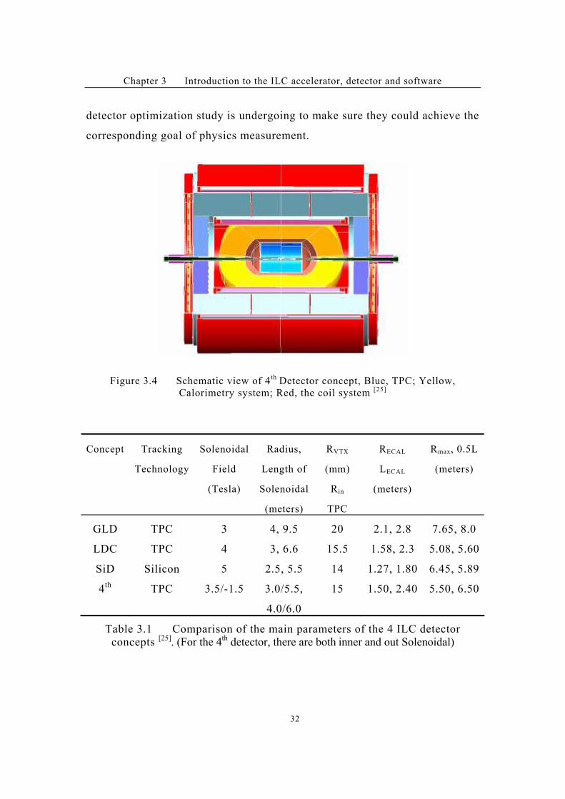
As a brief summary of the introduction to these 4 concepts, we list the
main parameters of these 4 concepts in Table 3.1. All of those 4 concepts have
been simulated in corresponding simulation software, the full simulation and
Chapter 3 Introduction to the ILC accelerator, detector and software
32
detector optimization study is undergoing to make sure they could achieve the
corresponding goal of physics measurement.
Figure 3.4 Schematic view of 4th Detector concept, Blue, TPC; Yellow,
Calorimetry system; Red, the coil system [25]
Concept Tracking
Technology
Solenoidal
Field
(Tesla)
Radius,
Length of
Solenoidal
(meters)
RVTX
(mm)
Rin
TPC
RECAL
LECAL
(meters)
Rmax, 0.5L
(meters)
GLD TPC 3 4, 9.5 20 2.1, 2.8 7.65, 8.0
LDC TPC 4 3, 6.6 15.5 1.58, 2.3 5.08, 5.60
SiD Silicon 5 2.5, 5.5 14 1.27, 1.80 6.45, 5.89
4th
TPC 3.5/-1.5 3.0/5.5,
4.0/6.0
15 1.50, 2.40 5.50, 6.50
Table 3.1 Comparison of the main parameters of the 4 ILC detector
concepts [25]
. (For the 4th
detector, there are both inner and out Solenoidal)
Chapter 3 Introduction to the ILC accelerator, detector and software
33
3.3 The emergence of the ILD concept group and current status of the
ILD detector optimization study
Because the LDC and GLD concepts shall many things in common, it was
decided to merge these two concepts into one, thus forming the ILD concept group[26]
.
The ILD group attempts to search for an optimized design of the ILC detector with
the detector optimization study.
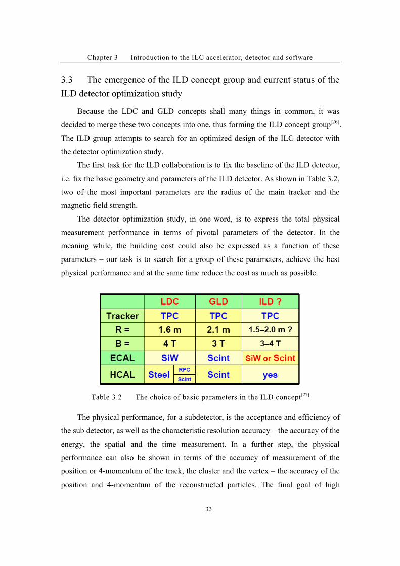
The first task for the ILD collaboration is to fix the baseline of the ILD detector,
i.e. fix the basic geometry and parameters of the ILD detector. As shown in Table 3.2,
two of the most important parameters are the radius of the main tracker and the
magnetic field strength.
The detector optimization study, in one word, is to express the total physical
measurement performance in terms of pivotal parameters of the detector. In the
meaning while, the building cost could also be expressed as a function of these
parameters – our task is to search for a group of these parameters, achieve the best
physical performance and at the same time reduce the cost as much as possible.
Table 3.2 The choice of basic parameters in the ILD concept[27]
The physical performance, for a subdetector, is the acceptance and efficiency of
the sub detector, as well as the characteristic resolution accuracy – the accuracy of the
energy, the spatial and the time measurement. In a further step, the physical
performance can also be shown in terms of the accuracy of measurement of the
position or 4-momentum of the track, the cluster and the vertex – the accuracy of the
position and 4-momentum of the reconstructed particles. The final goal of high
Chapter 3 Introduction to the ILC accelerator, detector and software
34
energy physics experiment is to calculate some parameters from the physical model,
like the mass and decay branching ratio of the Higgs particle, these parameters could
be expressed as a function of the 4-momentum of the associated reconstructed particle.
The most important questions about the detector R & D are: Could we measure these
parameters? What accuracy could we achieve with current detector concepts?
In practical, the detector optimization is a complex process. It is very hard to
express directly the physical performance in term of the characteristic parameters of
the detector (while the cost estimation is usually much simpler). The Monte Carlo
simulation is needed (or some fast simulation tools based on the experiment or full
simulation result) to get the detector performance with certain detector parameters. In
principle, we could use the simulation tools to scan over all the parameter spaces with
certain step length – but this is almost impossible with our current computing
capability: for the full simulation approximately we could simulate one event with
one CPU in one minute – while we have many benchmark channels with at least 10k
events each – these requirements on the computing resource could not be achieved
even with the support of the grid technique. The simulation work needs to be
organized in some priority (of those parameters), replace the whole parameter space
scanning with a linear scanning, and save a lot of machine time.
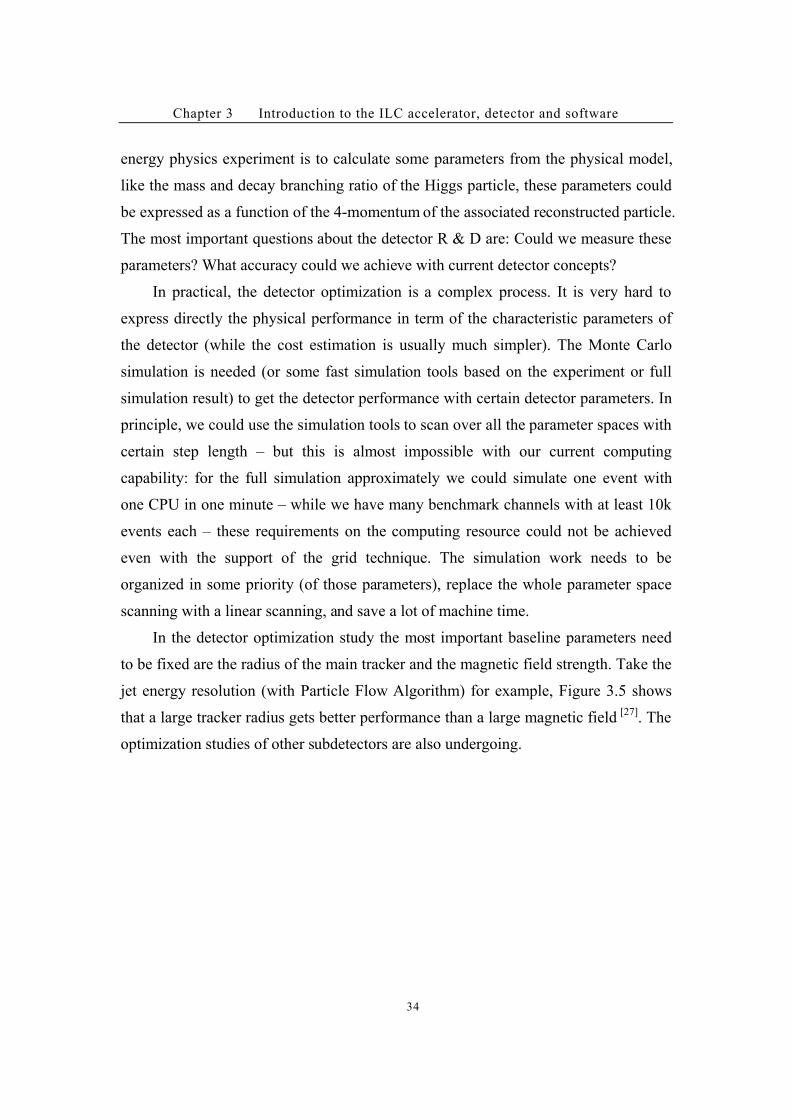
In the detector optimization study the most important baseline parameters need
to be fixed are the radius of the main tracker and the magnetic field strength. Take the
jet energy resolution (with Particle Flow Algorithm) for example, Figure 3.5 shows
that a large tracker radius gets better performance than a large magnetic field [27]
. The
optimization studies of other subdetectors are also undergoing.
Chapter 3 Introduction to the ILC accelerator, detector and software
35
Figure 3.5 Accuracy of jet energy resolution vary with TPC radius and magnetic
field strength [27]
The other strategy that the ILD optimization study adopts is to create an official
database to avoid simple repetition of works. The grid computing and storing tools
play an important role in this strategy. All the members of the ILD collaboration have
access to the database. The database includes all the data generated or used in the full
simulation study with given detector geometry, the generator file, the simulated
detector hits, the reconstructed physical events, etc. And for the reconstructed
physical events, there exist at least two versions, one minimal version which contains
only the MC truth and the reconstructed particles information, and a maximal version
which contains all the mediate collections in the simulation & reconstruction process.
As we can imagine, the minimal version of reconstructed files is very convenient for
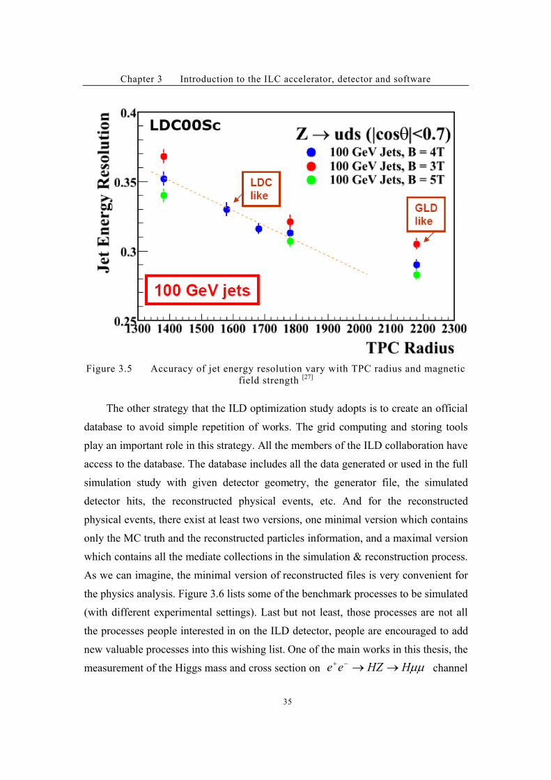
the physics analysis. Figure 3.6 lists some of the benchmark processes to be simulated
(with different experimental settings). Last but not least, those processes are not all
the processes people interested in on the ILD detector, people are encouraged to add
new valuable processes into this wishing list. One of the main works in this thesis, the
measurement of the Higgs mass and cross section on !!HHZee ""#$ channel
Chapter 3 Introduction to the ILC accelerator, detector and software
36
could also be regarded as part of the ILD detector optimization study.
Figure 3.6 Benchmark processes in the ILD detector optimization study [27]
Until now, the ILD detector optimization study is well organized and progresses
smoothly. The ILD Collaboration has a weekly phone meeting and keeps
upgrading/maintaining the software system. We believe that in the foreseen future,
we will have a more reliable, realistic and good performance detector concept.
3.4 Introduction to the LDC01_Sc concept
Our full simulation study on the Higgs mass measurement is based on the
detector concept LDC01_Sc [28]
. It is a minimal version of all the LDC detector
concepts, which is slightly smaller in size than the original version LDC00 – for the
TPC, there are only 184 layers instead of 200 layers (as in LDC00). There is no SET
or ETD in between the TPC and the ECAL, and no ! detector installed in the YOKE.
The sensor in the HCAL is scintillator (that’s why we have a “Sc” in its name, an
alternative choice is to use the RPC as the HCAL sensor). The structure of the
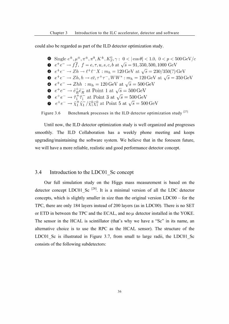
LDC01_Sc is illustrated in Figure 3.7, from small to large radii, the LDC01_Sc
consists of the following subdetectors:
Chapter 3 Introduction to the ILC accelerator, detector and software
37
Figure 3.7 LDC01_Sc concept (with a 50GeV # shot at 80o polar angle)
The tracking system: including a 5-layer silicon-pixel vertex detector (VTX), a
2-layer silicon inner tracker (SIT) and a 184-layer TPC. To ensure good track
momentum resolution at small polar angle, there exist 7 pairs of front tracking disks
based also on silicon strips pixel technique and the front chambers of TPC in the
forward region.
The calorimetry system: an ECAL with silicon-tungsten sandwich structure. The
ECAL is divided into 30 layers longitudinally, and segmented into 1cm#1cm cells
transversely. The HCAL has Iron-Scintillator sandwich structure, and divided into 40
layers longitudinally, while transversely segmented into 3cm#3cm cells for inner
layers, and 6cm#6cm or 12cm#12cm for the outer layers.
The coil and YOKE system: The superconductive coil creates a 4-Tesla
longitudinal magnetic field in the inner part of the detector. No # tracker has been
installed into the YOKE: the YOKE only plays the rule of flux return.
Now let’s discuss the tracking and calorimetry system.
Chapter 3 Introduction to the ILC accelerator, detector and software
38
3.4.1 Tracking System
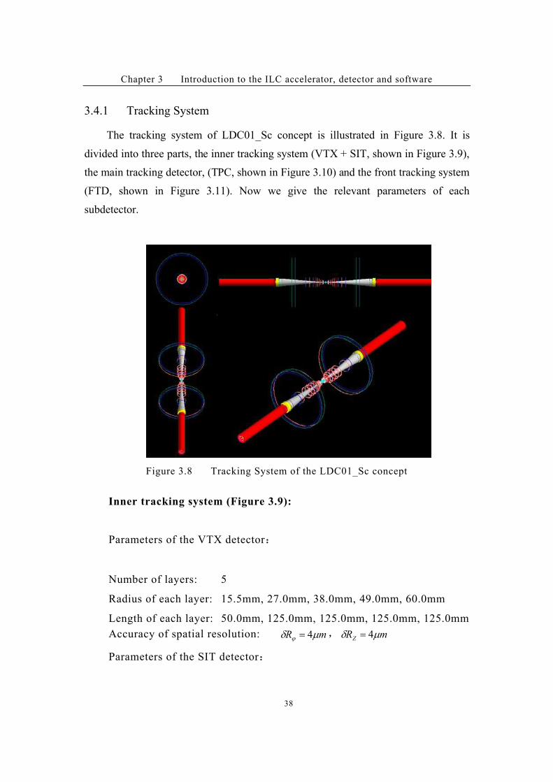
The tracking system of LDC01_Sc concept is illustrated in Figure 3.8. It is
divided into three parts, the inner tracking system (VTX + SIT, shown in Figure 3.9),
the main tracking detector, (TPC, shown in Figure 3.10) and the front tracking system
(FTD, shown in Figure 3.11). Now we give the relevant parameters of each
subdetector.
Figure 3.8 Tracking System of the LDC01_Sc concept
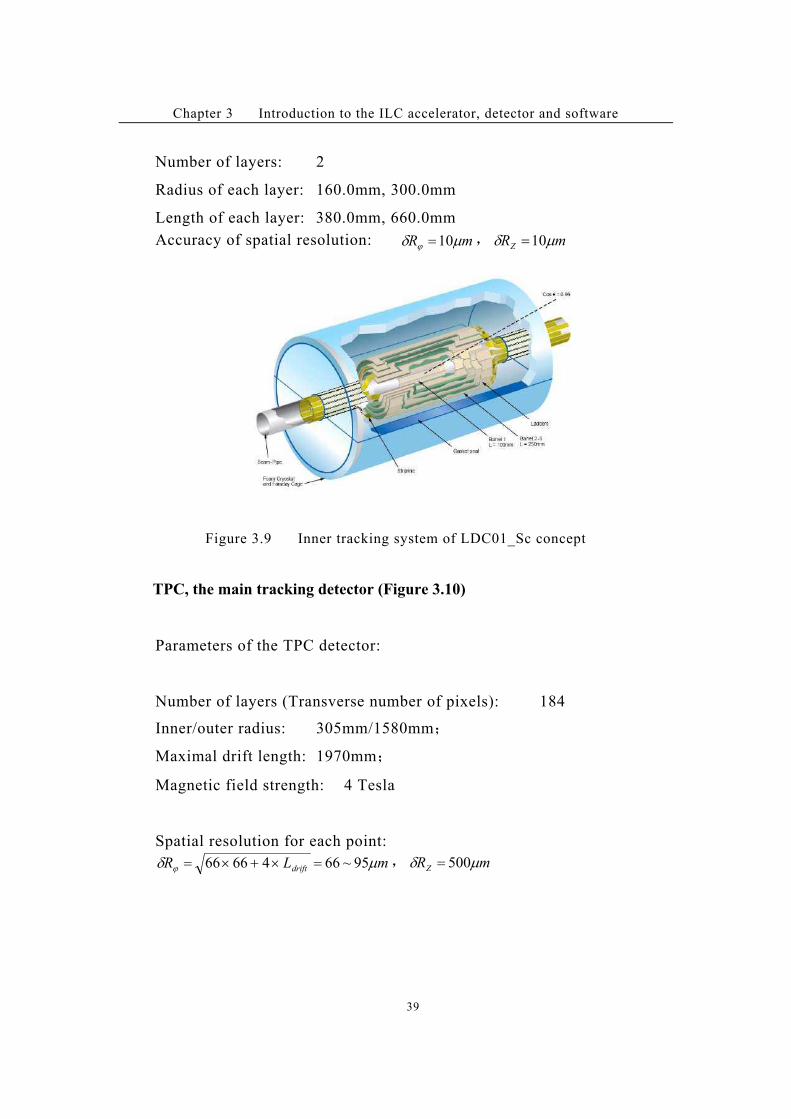
Inner tracking system (Figure 3.9):
Parameters of the VTX detector$
Number of layers: 5
Radius of each layer: 15.5mm, 27.0mm, 38.0mm, 49.0mm, 60.0mm
Length of each layer: 50.0mm, 125.0mm, 125.0mm, 125.0mm, 125.0mm
Accuracy of spatial resolution: mR !1 2 4' " mRZ !1 4'
Parameters of the SIT detector$
Chapter 3 Introduction to the ILC accelerator, detector and software
39
Number of layers: 2
Radius of each layer: 160.0mm, 300.0mm
Length of each layer: 380.0mm, 660.0mm
Accuracy of spatial resolution: mR !1 2 10' " mRZ !1 10'
Figure 3.9 Inner tracking system of LDC01_Sc concept
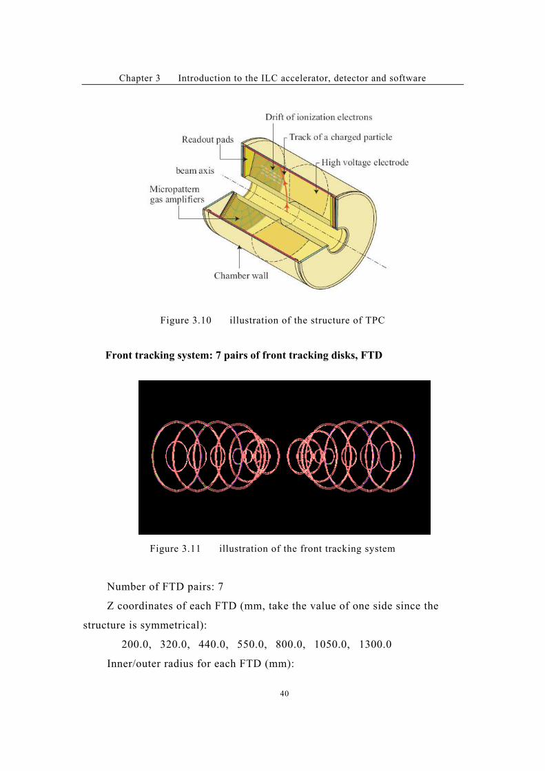
TPC, the main tracking detector (Figure 3.10)
Parameters of the TPC detector:
Number of layers (Transverse number of pixels): 184
Inner/outer radius: 305mm/1580mm%
Maximal drift length: 1970mm%
Magnetic field strength: 4 Tesla
Spatial resolution for each point:
mLR drift !1 2 95~6646666 '/$/' " mRZ !1 500'
Chapter 3 Introduction to the ILC accelerator, detector and software
40
Figure 3.10 illustration of the structure of TPC
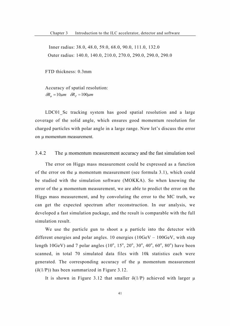
Front tracking system: 7 pairs of front tracking disks, FTD
Figure 3.11 illustration of the front tracking system
Number of FTD pairs: 7
Z coordinates of each FTD (mm, take the value of one side since the
structure is symmetrical):
200.0, 320.0, 440.0, 550.0, 800.0, 1050.0, 1300.0
Inner/outer radius for each FTD (mm):
Chapter 3 Introduction to the ILC accelerator, detector and software
41
Inner radius: 38.0, 48.0, 59.0, 68.0, 90.0, 111.0, 132.0
Outer radius: 140.0, 140.0, 210.0, 270.0, 290.0, 290.0, 290.0
FTD thickness: 0.3mm
Accuracy of spatial resolution:
mR !1 2 10' mRZ !1 100'
LDC01_Sc tracking system has good spatial resolution and a large
coverage of the solid angle, which ensures good momentum resolution for
charged particles with polar angle in a large range. Now let’s discuss the error
on # momentum measurement.
3.4.2 The # momentum measurement accuracy and the fast simulation tool !
The error on Higgs mass measurement could be expressed as a function
of the error on the # momentum measurement (see formula 3.1), which could
be studied with the simulation software (MOKKA). So when knowing the
error of the # momentum measurement, we are able to predict the error on the
Higgs mass measurement, and by convoluting the error to the MC truth, we
can get the expected spectrum after reconstruction. In our analysis, we
developed a fast simulation package, and the result is comparable with the full
simulation result.
We use the particle gun to shoot a # particle into the detector with
different energies and polar angles. 10 energies (10GeV – 100GeV, with step
length 10GeV) and 7 polar angles (10o, 15
o, 20
o, 30
o, 40
o, 60
o, 80
o) have been
scanned, in total 70 simulated data files with 10k statistics each were
generated. The corresponding accuracy of the # momentum measurement
(&(1/P)) has been summarized in Figure 3.12.
It is shown in Figure 3.12 that smaller &(1/P) achieved with larger #
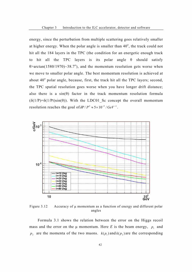
Chapter 3 Introduction to the ILC accelerator, detector and software
42
energy, since the perturbation from multiple scattering goes relatively smaller
at higher energy. When the polar angle is smaller than 40o, the track could not
hit all the 184 layers in the TPC (the condition for an energetic enough track
to hit all the TPC layers is its polar angle ' should satisfy
'>arctan(1580/1970)~38.7o), and the momentum resolution gets worse when
we move to smaller polar angle. The best momentum resolution is achieved at
about 40o polar angle, because, first, the track hit all the TPC layers; second,
the TPC spatial resolution goes worse when you have longer drift distance;
also there is a sin(') factor in the track momentum resolution formula
(&(1/P)=&(1/Pt)sin(')). With the LDC01_Sc concept the overall momentum
resolution reaches the goal of 152 /105/ ##/0 GeVPP1 .
Figure 3.12 Accuracy of # momentum as a function of energy and different polar
angles
Formula 3.1 shows the relation between the error on the Higgs recoil
mass and the error on the # momentum. Here E is the beam energy, 1p and
2p are the momenta of the two muons. )( 1pk and )( 2pk are the corresponding
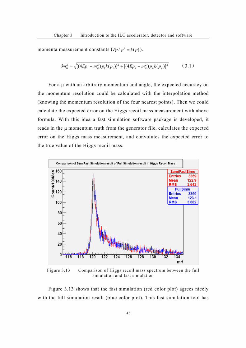
Chapter 3 Introduction to the ILC accelerator, detector and software
43
momenta measurement constants ( )(/ 2 pkpp '1 ).
2
22
2
2
2
11
2
1
2 )]()4[()]()4[( pkpmEppkpmEpm ZZH #$#'1 &3.1'
For a # with an arbitrary momentum and angle, the expected accuracy on
the momentum resolution could be calculated with the interpolation method
(knowing the momentum resolution of the four nearest points). Then we could
calculate the expected error on the Higgs recoil mass measurement with above
formula. With this idea a fast simulation software package is developed, it
reads in the # momentum truth from the generator file, calculates the expected
error on the Higgs mass measurement, and convolutes the expected error to
the true value of the Higgs recoil mass.
Figure 3.13 Comparison of Higgs recoil mass spectrum between the full
simulation and fast simulation
Figure 3.13 shows that the fast simulation (red color plot) agrees nicely
with the full simulation result (blue color plot). This fast simulation tool has
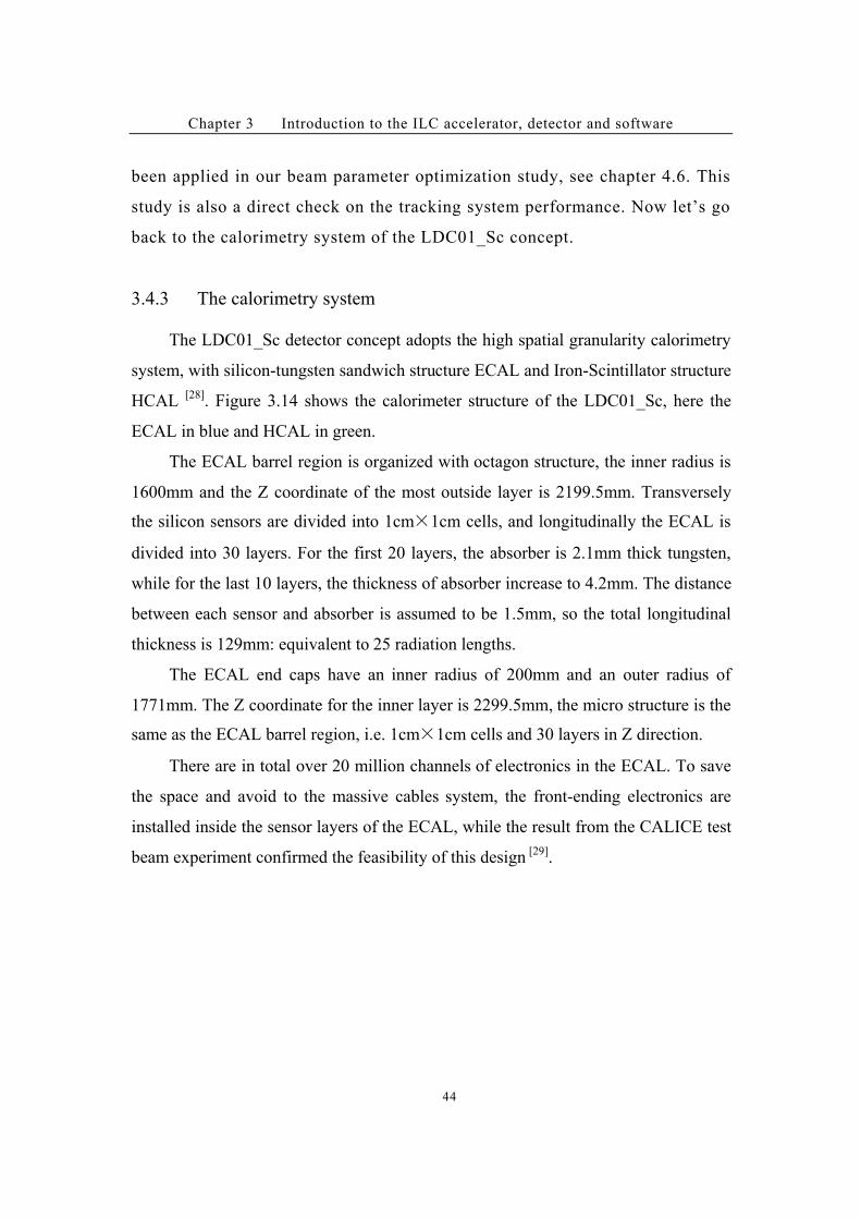
Chapter 3 Introduction to the ILC accelerator, detector and software
44
been applied in our beam parameter optimization study, see chapter 4.6. This
study is also a direct check on the tracking system performance. Now let’s go
back to the calorimetry system of the LDC01_Sc concept.
3.4.3 The calorimetry system
The LDC01_Sc detector concept adopts the high spatial granularity calorimetry
system, with silicon-tungsten sandwich structure ECAL and Iron-Scintillator structure
HCAL [28]
. Figure 3.14 shows the calorimeter structure of the LDC01_Sc, here the
ECAL in blue and HCAL in green.
The ECAL barrel region is organized with octagon structure, the inner radius is
1600mm and the Z coordinate of the most outside layer is 2199.5mm. Transversely
the silicon sensors are divided into 1cm#1cm cells, and longitudinally the ECAL is
divided into 30 layers. For the first 20 layers, the absorber is 2.1mm thick tungsten,
while for the last 10 layers, the thickness of absorber increase to 4.2mm. The distance
between each sensor and absorber is assumed to be 1.5mm, so the total longitudinal
thickness is 129mm: equivalent to 25 radiation lengths.
The ECAL end caps have an inner radius of 200mm and an outer radius of
1771mm. The Z coordinate for the inner layer is 2299.5mm, the micro structure is the
same as the ECAL barrel region, i.e. 1cm#1cm cells and 30 layers in Z direction.
There are in total over 20 million channels of electronics in the ECAL. To save
the space and avoid to the massive cables system, the front-ending electronics are
installed inside the sensor layers of the ECAL, while the result from the CALICE test
beam experiment confirmed the feasibility of this design [29]
.
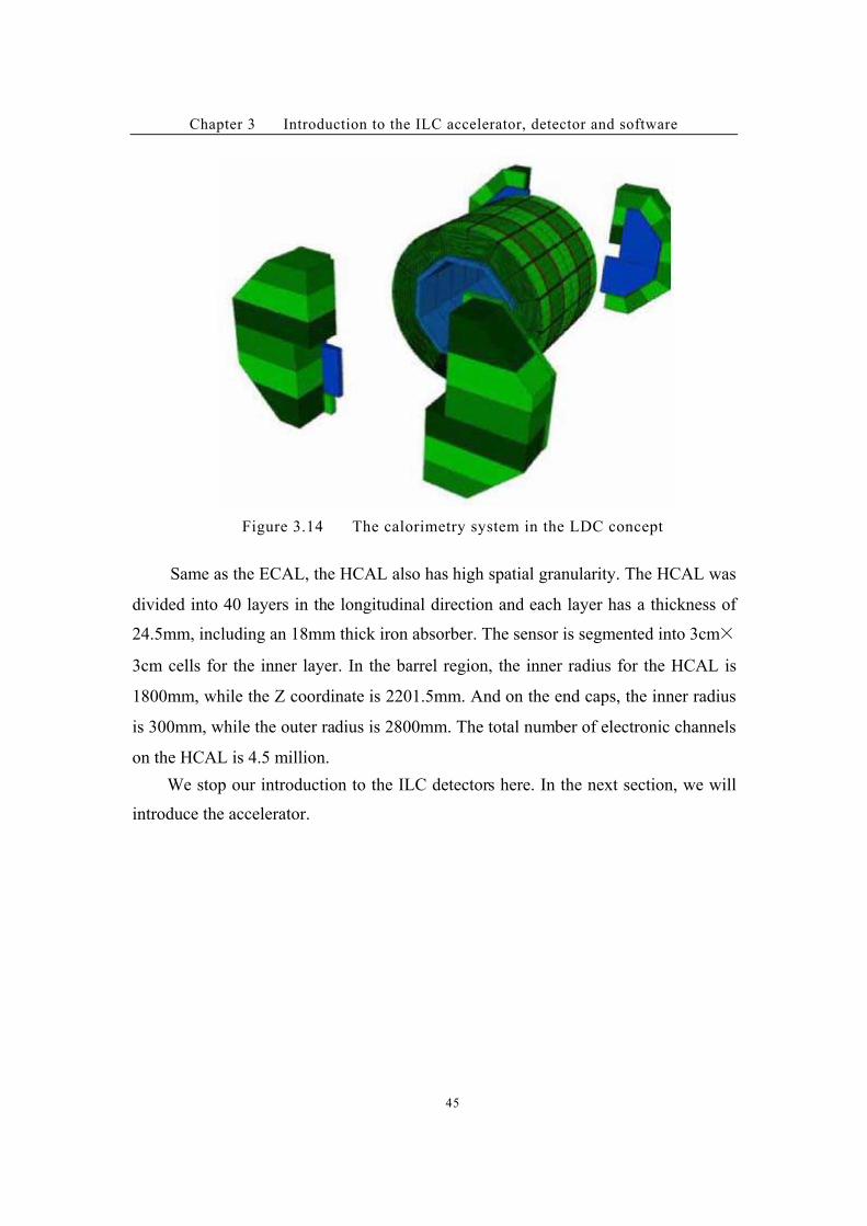
Chapter 3 Introduction to the ILC accelerator, detector and software
45
Figure 3.14 The calorimetry system in the LDC concept
Same as the ECAL, the HCAL also has high spatial granularity. The HCAL was
divided into 40 layers in the longitudinal direction and each layer has a thickness of
24.5mm, including an 18mm thick iron absorber. The sensor is segmented into 3cm#
3cm cells for the inner layer. In the barrel region, the inner radius for the HCAL is
1800mm, while the Z coordinate is 2201.5mm. And on the end caps, the inner radius
is 300mm, while the outer radius is 2800mm. The total number of electronic channels
on the HCAL is 4.5 million.
We stop our introduction to the ILC detectors here. In the next section, we will
introduce the accelerator.
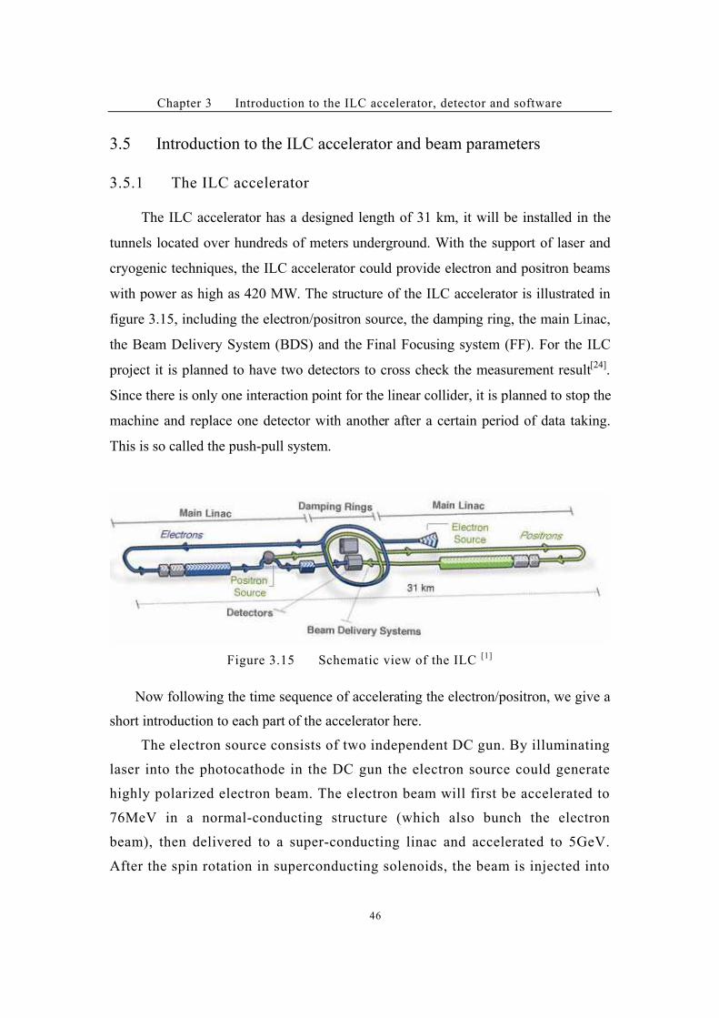
Chapter 3 Introduction to the ILC accelerator, detector and software
46
3.5 Introduction to the ILC accelerator and beam parameters
3.5.1 The ILC accelerator!
The ILC accelerator has a designed length of 31 km, it will be installed in the
tunnels located over hundreds of meters underground. With the support of laser and
cryogenic techniques, the ILC accelerator could provide electron and positron beams
with power as high as 420 MW. The structure of the ILC accelerator is illustrated in
figure 3.15, including the electron/positron source, the damping ring, the main Linac,
the Beam Delivery System (BDS) and the Final Focusing system (FF). For the ILC
project it is planned to have two detectors to cross check the measurement result[24]
.
Since there is only one interaction point for the linear collider, it is planned to stop the
machine and replace one detector with another after a certain period of data taking.
This is so called the push-pull system.
Figure 3.15 Schematic view of the ILC [1]
Now following the time sequence of accelerating the electron/positron, we give a
short introduction to each part of the accelerator here.
The electron source consists of two independent DC gun. By illuminating
laser into the photocathode in the DC gun the electron source could generate
highly polarized electron beam. The electron beam will first be accelerated to
76MeV in a normal-conducting structure (which also bunch the electron
beam), then delivered to a super-conducting linac and accelerated to 5GeV.
After the spin rotation in superconducting solenoids, the beam is injected into
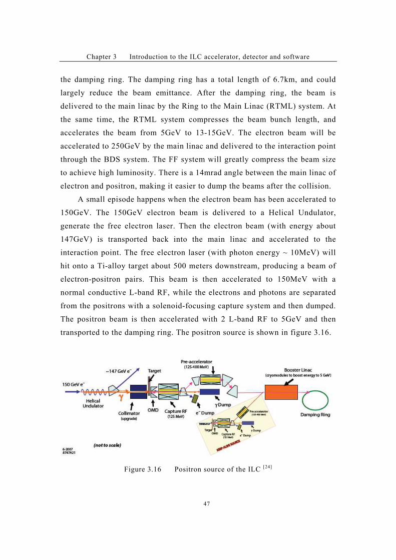
Chapter 3 Introduction to the ILC accelerator, detector and software
47
the damping ring. The damping ring has a total length of 6.7km, and could
largely reduce the beam emittance. After the damping ring, the beam is
delivered to the main linac by the Ring to the Main Linac (RTML) system. At
the same time, the RTML system compresses the beam bunch length, and
accelerates the beam from 5GeV to 13-15GeV. The electron beam will be
accelerated to 250GeV by the main linac and delivered to the interaction point
through the BDS system. The FF system will greatly compress the beam size
to achieve high luminosity. There is a 14mrad angle between the main linac of
electron and positron, making it easier to dump the beams after the collision.
A small episode happens when the electron beam has been accelerated to
150GeV. The 150GeV electron beam is delivered to a Helical Undulator,
generate the free electron laser. Then the electron beam (with energy about
147GeV) is transported back into the main linac and accelerated to the
interaction point. The free electron laser (with photon energy ~ 10MeV) will
hit onto a Ti-alloy target about 500 meters downstream, producing a beam of
electron-positron pairs. This beam is then accelerated to 150MeV with a
normal conductive L-band RF, while the electrons and photons are separated
from the positrons with a solenoid-focusing capture system and then dumped.
The positron beam is then accelerated with 2 L-band RF to 5GeV and then
transported to the damping ring. The positron source is shown in figure 3.16.
Figure 3.16 Positron source of the ILC [24]

Chapter 3 Introduction to the ILC accelerator, detector and software
48
The 9-Cell RF cavities (Figure 3.17) constructed with pure niobium
material play a central role in the beam acceleration. Its working frequency is
1.3GHz, the microwave is injected into the cavity and creates extremely
strong electro field (34.5MV/m). The RF cavities are supposed to work with
2K temperature (requirement from super conductive) so it is totally embedded
in the liquid helium shower.
Figure 3.17 9-Cell RF cavities [24]
The main linac is constructed with 37.956 meter long RF units (Figure
3.18), each consists of three SCRF cryomodules and has in total 26 nine-cell
cavities. Each RF unit has an independent RF source, which includes a
high-voltage (120 kV) modulator, a 10 MW multi-beam klystron and a
waveguide system. The main linac for the positron beam has 278 RF units,
while there are 282 RF units for the electron main linac: since the electron
beam loses about 3GeV energy in the positron source.
According to the RDR, the main linac components are located in two
paralleled tunnels, an accelerator tunnel and a service tunnel, each of which
has an interior diameter of 4.5 meters (Figure 3.19). The RF source is housed
mainly in the service tunnel to facilitate the maintenance and limit radiation
exposure. The tunnels are located several hundreds meters underground.
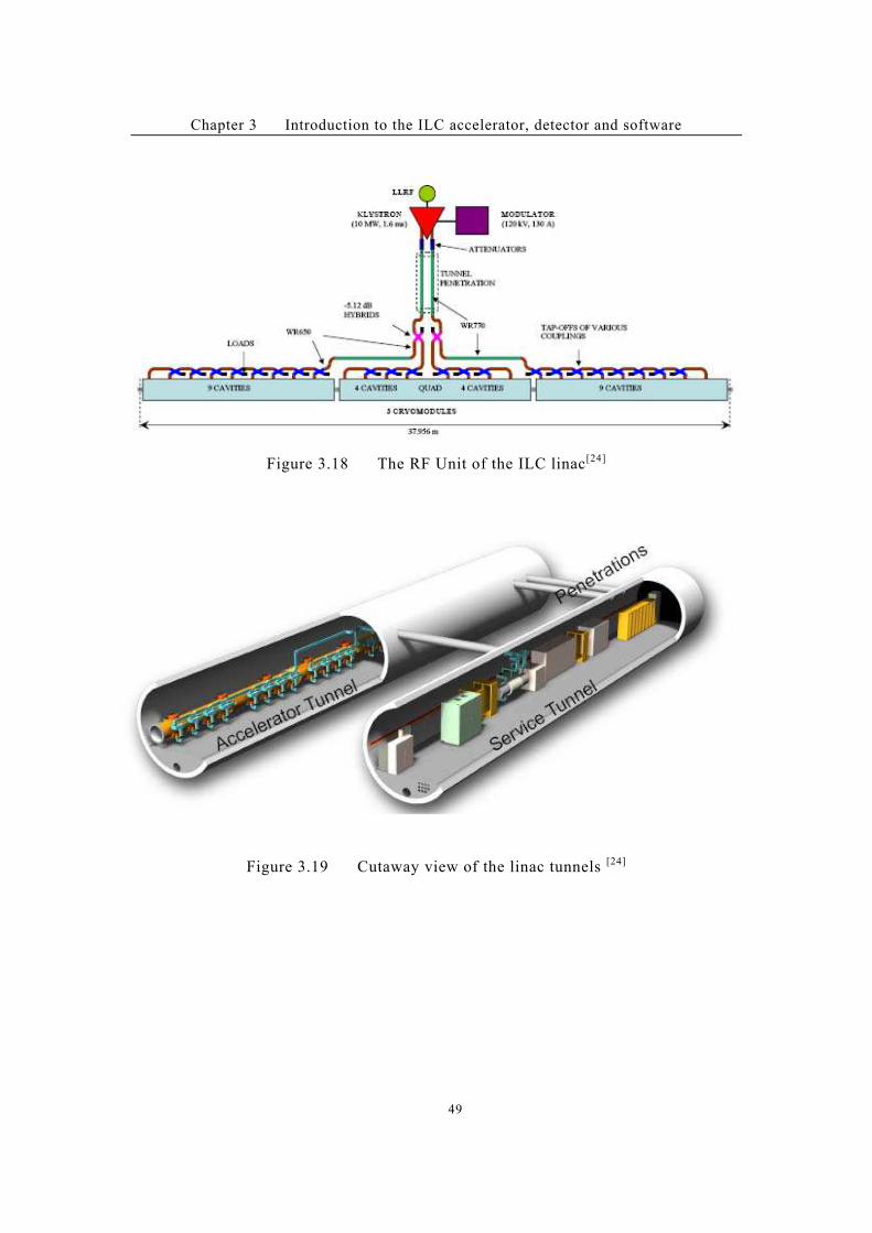
Chapter 3 Introduction to the ILC accelerator, detector and software
49
Figure 3.18 The RF Unit of the ILC linac[24]
Figure 3.19 Cutaway view of the linac tunnels [24]
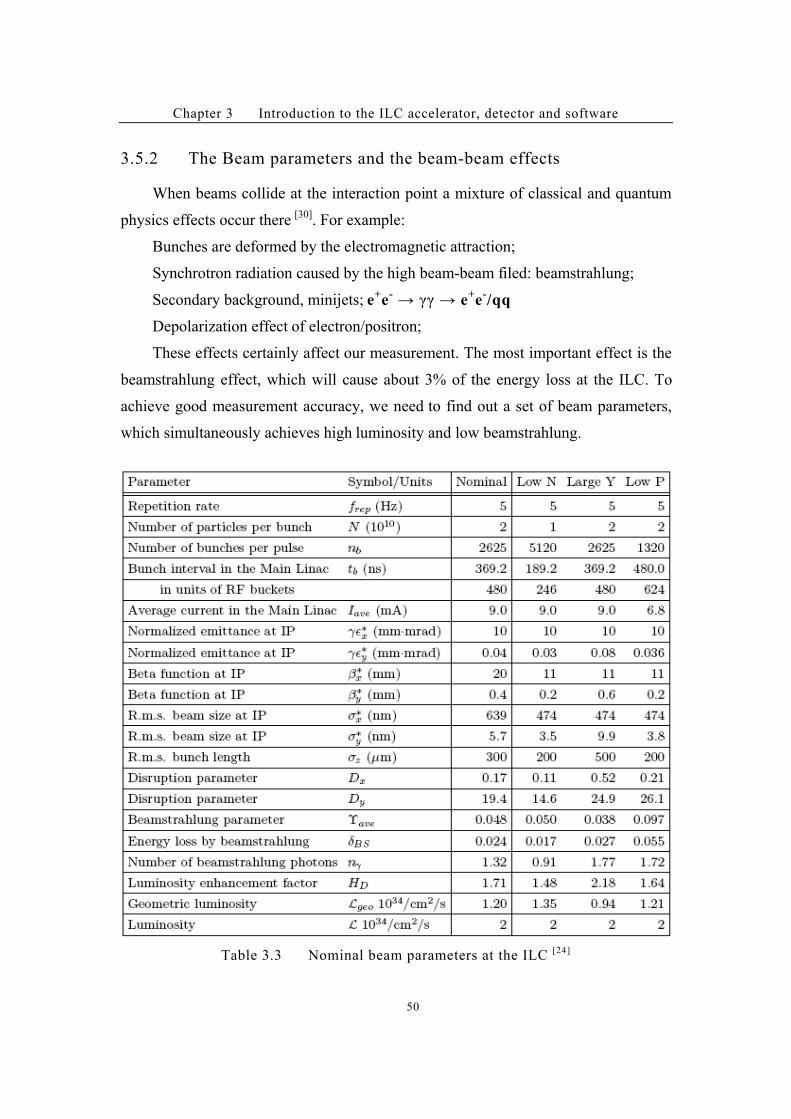
Chapter 3 Introduction to the ILC accelerator, detector and software
50
3.5.2 The Beam parameters and the beam-beam effects
When beams collide at the interaction point a mixture of classical and quantum
physics effects occur there [30]
. For example:
Bunches are deformed by the electromagnetic attraction;
Synchrotron radiation caused by the high beam-beam filed: beamstrahlung;
Secondary background, minijets; e+e
- ( )) ( e
+e
Depolarization effect of electron/positron;
These effects certainly affect our measurement. The most important effect is the
beamstrahlung effect, which will cause about 3% of the energy loss at the ILC. To
achieve good measurement accuracy, we need to find out a set of beam parameters,
which simultaneously achieves high luminosity and low beamstrahlung.
Table 3.3 Nominal beam parameters at the ILC [24]

Chapter 3 Introduction to the ILC accelerator, detector and software
51
Table 3.3 shows the nominal beam parameters at 500GeV center-of-mass
energy at the ILC. In the Z direction, the beam particles are formed into
bunches and then grouped into bunch trains. For the nominal beam parameter,
a bunch consists of 2#1010
(N) particles and has a length of 300 #m near the
interaction point. The distance between bunches is 110.76 meters (369.2ns, tb). 2625
(nb) bunches form a bunch train, which has a length of 290.7km (equivalent to ~1ms
in time). The frequency of the bunch train is 5Hz (fr), means that there is 200ms
distance between bunch trains.
With the above information, we can easily calculate the beam current at the ILC:
.
The power of the electron and position beams is 420MW for 500GeV
center-of-mass energy. As we mentioned in the accelerator chapter, the main linac
consists of 560 RF sources (10MW each), so the total energy transition efficiency for
the main linac is roughly 7-8%.
The basic parameters to describe the geometry of bunch are the emittance and
beta function in both X and Y direction. The emittance has a dimension of meter,
which means the area of angular-position phase space the particles in a bunch have
occupied (1 *). So lower emittance means the bunch particles are more concentrated
in the phase space. A more straightforward description for the spatial concentration of
bunch particles is *x(*y, which means the geometrical size of the bunch. There has a
simple relation with the beta function and emittance: 3(4) /* .
Disruption describes the effect of the EM field surrounding each bunch during
the collision: each beam acting as a thin focusing lens and changing the opposite
beam trajectory. Disruption is determined by *x(*y in the following way [30]
:
mAN
FnNf
A
br 84.010*023.6
96500*2625*5*10*2*22
23
10
'''I
)(
2
,
,
yxyx
zeyx
NrD
))3)
)
$5
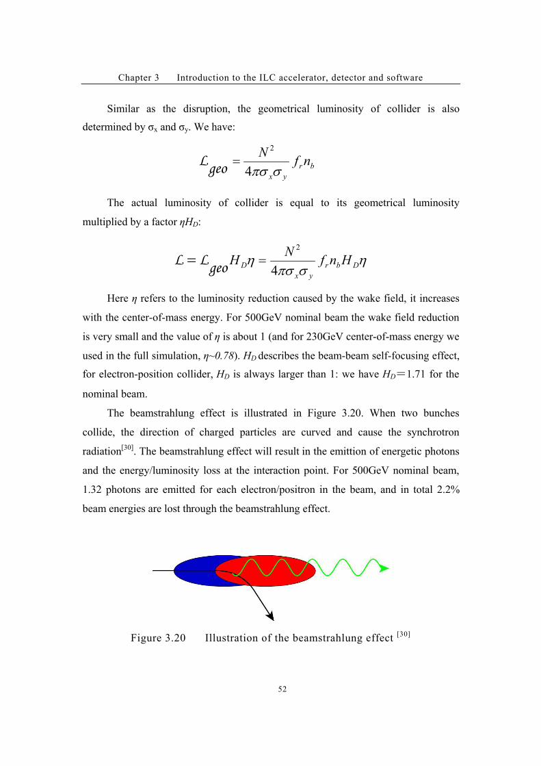
Chapter 3 Introduction to the ILC accelerator, detector and software
52
Similar as the disruption, the geometrical luminosity of collider is also
determined by *x and *y. We have:
The actual luminosity of collider is equal to its geometrical luminosity
multiplied by a factor !HD:
Here ! refers to the luminosity reduction caused by the wake field, it increases
with the center-of-mass energy. For 500GeV nominal beam the wake field reduction
is very small and the value of ! is about 1 (and for 230GeV center-of-mass energy we
used in the full simulation, !~0.78). HD describes the beam-beam self-focusing effect,
for electron-position collider, HD is always larger than 1: we have HD)1.71 for the
nominal beam.
The beamstrahlung effect is illustrated in Figure 3.20. When two bunches
collide, the direction of charged particles are curved and cause the synchrotron
radiation[30]
. The beamstrahlung effect will result in the emittion of energetic photons
and the energy/luminosity loss at the interaction point. For 500GeV nominal beam,
1.32 photons are emitted for each electron/positron in the beam, and in total 2.2%
beam energies are lost through the beamstrahlung effect.
Figure 3.20 Illustration of the beamstrahlung effect [30]
br
yx
nfN
)6)4
2
'geoL
7)6)
7 Dbr
yx
D HnfN
H4
2
''geoLL
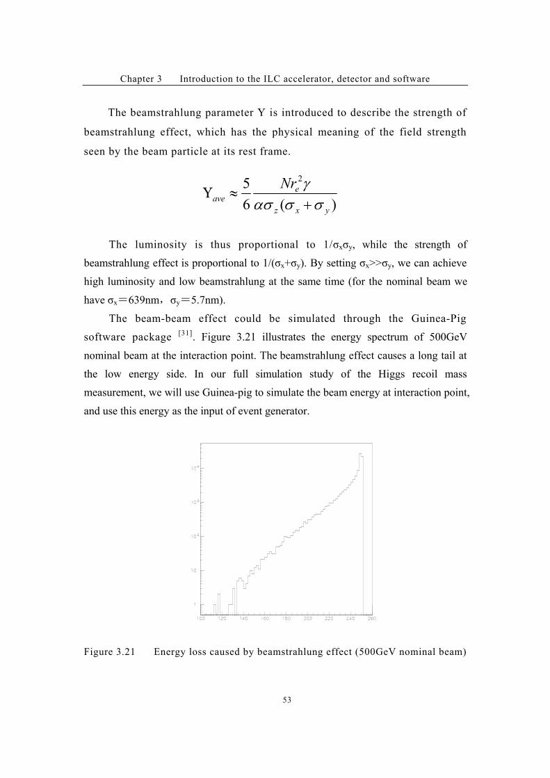
Chapter 3 Introduction to the ILC accelerator, detector and software
53
The beamstrahlung parameter Y is introduced to describe the strength of
beamstrahlung effect, which has the physical meaning of the field strength
seen by the beam particle at its rest frame.
The luminosity is thus proportional to 1/*x*y, while the strength of
beamstrahlung effect is proportional to 1/(*x+*y). By setting *x>>*y, we can achieve
high luminosity and low beamstrahlung at the same time (for the nominal beam we
have *x)639nm"*y)5.7nm).
The beam-beam effect could be simulated through the Guinea-Pig
software package [31]
. Figure 3.21 illustrates the energy spectrum of 500GeV
nominal beam at the interaction point. The beamstrahlung effect causes a long tail at
the low energy side. In our full simulation study of the Higgs recoil mass
measurement, we will use Guinea-pig to simulate the beam energy at interaction point,
and use this energy as the input of event generator.
Figure 3.21 Energy loss caused by beamstrahlung effect (500GeV nominal beam)
)(6
5 2
yxz
eave
Nr
))8)
3
$09
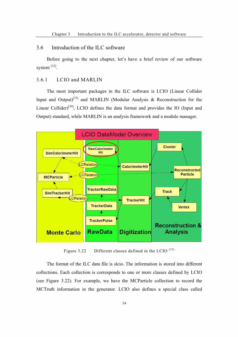
Chapter 3 Introduction to the ILC accelerator, detector and software
54
3.6 Introduction of the ILC software
Before going to the next chapter, let’s have a brief review of our software
system [32]
.
3.6.1 LCIO and MARLIN!
The most important packages in the ILC software is LCIO (Linear Collider
Input and Output)[33]
and MARLIN (Modular Analysis & Reconstruction for the
Linear Collider)[34]
, LCIO defines the data format and provides the IO (Input and
Output) standard, while MARLIN is an analysis framework and a module manager.
Figure 3.22 Different classes defined in the LCIO [35]
The format of the ILC data file is slcio. The information is stored into different
collections. Each collection is corresponds to one or more classes defined by LCIO
(see Figure 3.22). For example, we have the MCParticle collection to record the
MCTruth information in the generator. LCIO also defines a special class called
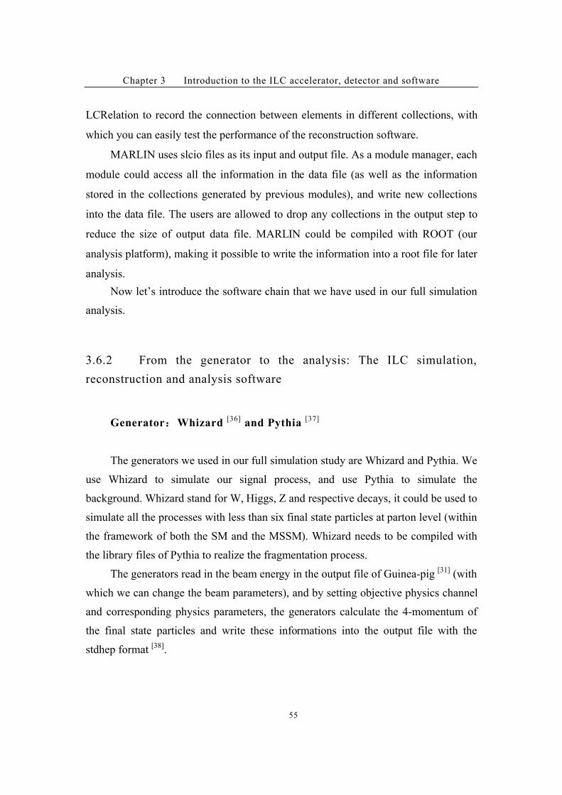
Chapter 3 Introduction to the ILC accelerator, detector and software
55
LCRelation to record the connection between elements in different collections, with
which you can easily test the performance of the reconstruction software.
MARLIN uses slcio files as its input and output file. As a module manager, each
module could access all the information in the data file (as well as the information
stored in the collections generated by previous modules), and write new collections
into the data file. The users are allowed to drop any collections in the output step to
reduce the size of output data file. MARLIN could be compiled with ROOT (our
analysis platform), making it possible to write the information into a root file for later
analysis.
Now let’s introduce the software chain that we have used in our full simulation
analysis.
3.6.2 From the generator to the analysis: The ILC simulation,
reconstruction and analysis software!
Generator$Whizard [36]
and Pythia [37]
The generators we used in our full simulation study are Whizard and Pythia. We
use Whizard to simulate our signal process, and use Pythia to simulate the
background. Whizard stand for W, Higgs, Z and respective decays, it could be used to
simulate all the processes with less than six final state particles at parton level (within
the framework of both the SM and the MSSM). Whizard needs to be compiled with
the library files of Pythia to realize the fragmentation process.
The generators read in the beam energy in the output file of Guinea-pig [31]
(with
which we can change the beam parameters), and by setting objective physics channel
and corresponding physics parameters, the generators calculate the 4-momentum of
the final state particles and write these informations into the output file with the
stdhep format [38]
.
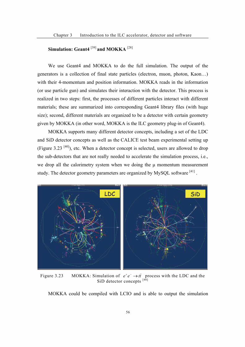
Chapter 3 Introduction to the ILC accelerator, detector and software
56
Simulation: Geant4 [39]
and MOKKA [28]
We use Geant4 and MOKKA to do the full simulation. The output of the
generators is a collection of final state particles (electron, muon, photon, Kaon…)
with their 4-momentum and position information. MOKKA reads in the information
(or use particle gun) and simulates their interaction with the detector. This process is
realized in two steps: first, the processes of different particles interact with different
materials; these are summarized into corresponding Geant4 library files (with huge
size); second, different materials are organized to be a detector with certain geometry
given by MOKKA (in other word, MOKKA is the ILC geometry plug-in of Geant4).
MOKKA supports many different detector concepts, including a set of the LDC
and SiD detector concepts as well as the CALICE test beam experimental setting up
(Figure 3.23 [40]
), etc. When a detector concept is selected, users are allowed to drop
the sub-detectors that are not really needed to accelerate the simulation process, i.e.,
we drop all the calorimetry system when we doing the # momentum measurement
study. The detector geometry parameters are organized by MySQL software [41]
.
Figure 3.23 MOKKA: Simulation of ttee "#$ process with the LDC and the
SiD detector concepts [40]
MOKKA could be compiled with LCIO and is able to output the simulation
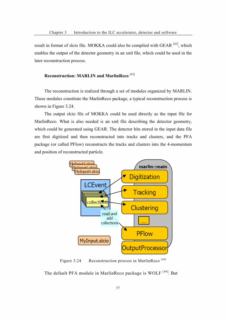
Chapter 3 Introduction to the ILC accelerator, detector and software
57
result in format of slcio file. MOKKA could also be compiled with GEAR [42]
, which
enables the output of the detector geometry in an xml file, which could be used in the
later reconstruction process.
Reconstruction: MARLIN and MarlinReco [43]
The reconstruction is realized through a set of modules organized by MARLIN.
These modules constitute the MarlinReco package, a typical reconstruction process is
shown in Figure 3.24.
The output slcio file of MOKKA could be used directly as the input file for
MarlinReco. What is also needed is an xml file describing the detector geometry,
which could be generated using GEAR. The detector hits stored in the input data file
are first digitized and then reconstructed into tracks and clusters, and the PFA
package (or called PFlow) reconstructs the tracks and clusters into the 4-momentum
and position of reconstructed particle.
Figure 3.24 Reconstruction process in MarlinReco [40]
The default PFA module in MarlinReco package is WOLF [44]
. But
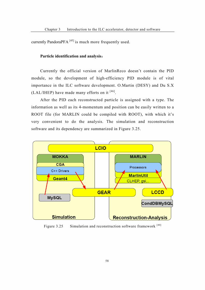
Chapter 3 Introduction to the ILC accelerator, detector and software
58
currently PandoraPFA [45]
is much more frequently used.
Particle identification and analysis$
Currently the official version of MarlinReco doesn’t contain the PID
module, so the development of high-efficiency PID module is of vital
importance in the ILC software development. O.Martin (DESY) and Du S.X
(LAL/IHEP) have made many efforts on it [46]
.
After the PID each reconstructed particle is assigned with a type. The
information as well as its 4-momentum and position can be easily written to a
ROOT file (for MARLIN could be compiled with ROOT), with which it’s
very convenient to do the analysis. The simulation and reconstruction
software and its dependency are summarized in Figure 3.25.
Figure 3.25 Simulation and reconstruction software framework [40]
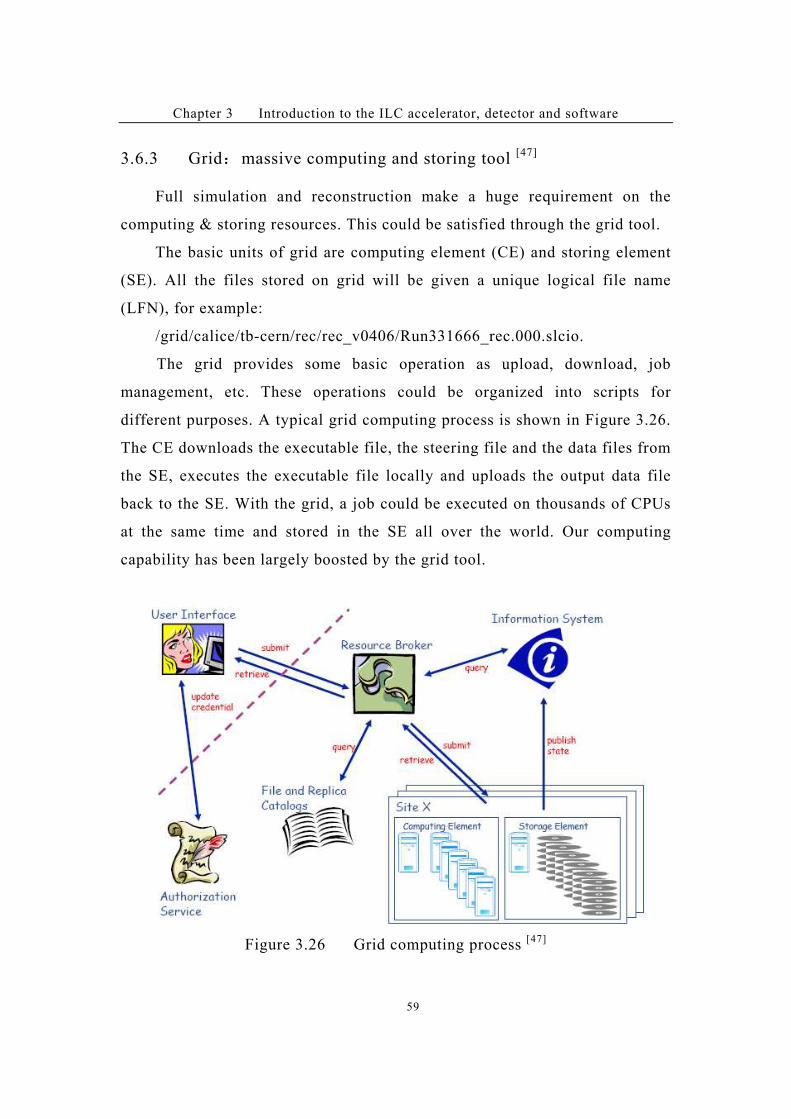
Chapter 3 Introduction to the ILC accelerator, detector and software
59
3.6.3 Grid"massive computing and storing tool [47]
!
Full simulation and reconstruction make a huge requirement on the
computing & storing resources. This could be satisfied through the grid tool.
The basic units of grid are computing element (CE) and storing element
(SE). All the files stored on grid will be given a unique logical file name
(LFN), for example:
/grid/calice/tb-cern/rec/rec_v0406/Run331666_rec.000.slcio.
The grid provides some basic operation as upload, download, job
management, etc. These operations could be organized into scripts for
different purposes. A typical grid computing process is shown in Figure 3.26.
The CE downloads the executable file, the steering file and the data files from
the SE, executes the executable file locally and uploads the output data file
back to the SE. With the grid, a job could be executed on thousands of CPUs
at the same time and stored in the SE all over the world. Our computing
capability has been largely boosted by the grid tool.
Figure 3.26 Grid computing process [47]
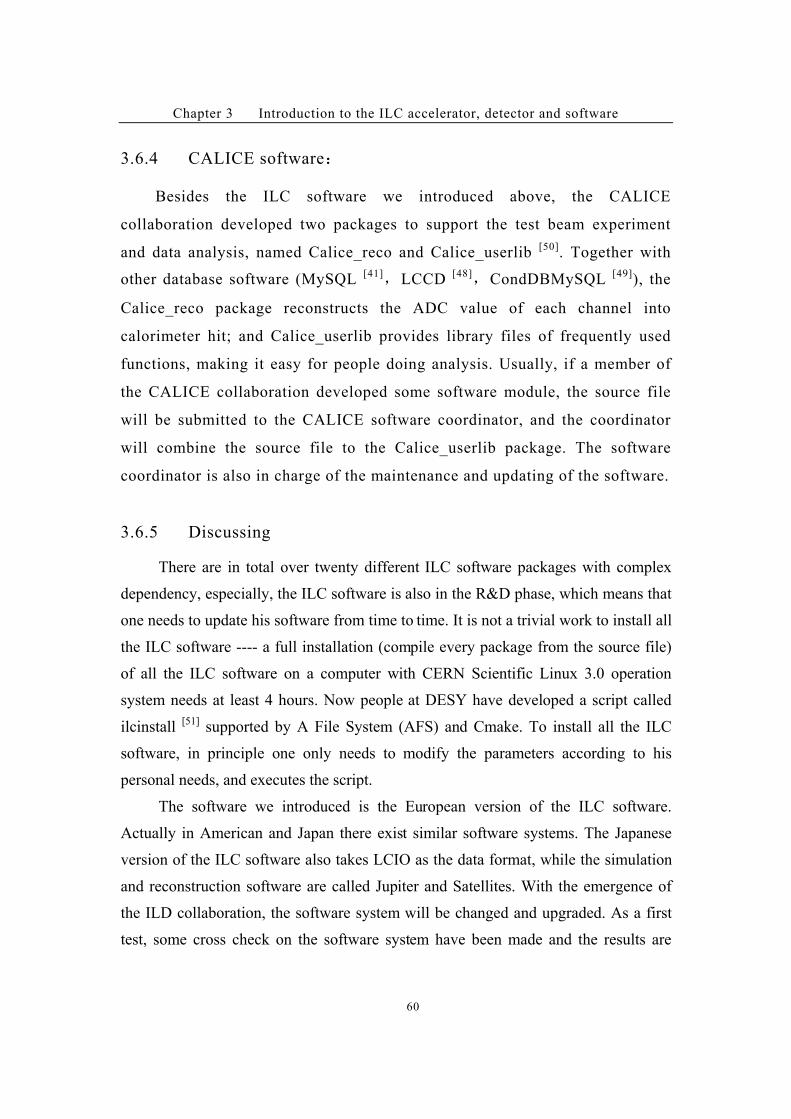
Chapter 3 Introduction to the ILC accelerator, detector and software
60
3.6.4 CALICE software"!
Besides the ILC software we introduced above, the CALICE
collaboration developed two packages to support the test beam experiment
and data analysis, named Calice_reco and Calice_userlib [50]
. Together with
other database software (MySQL [41]"LCCD
[48]"CondDBMySQL [49]
), the
Calice_reco package reconstructs the ADC value of each channel into
calorimeter hit; and Calice_userlib provides library files of frequently used
functions, making it easy for people doing analysis. Usually, if a member of
the CALICE collaboration developed some software module, the source file
will be submitted to the CALICE software coordinator, and the coordinator
will combine the source file to the Calice_userlib package. The software
coordinator is also in charge of the maintenance and updating of the software.
3.6.5 Discussing!
There are in total over twenty different ILC software packages with complex
dependency, especially, the ILC software is also in the R&D phase, which means that
one needs to update his software from time to time. It is not a trivial work to install all
the ILC software ---- a full installation (compile every package from the source file)
of all the ILC software on a computer with CERN Scientific Linux 3.0 operation
system needs at least 4 hours. Now people at DESY have developed a script called
ilcinstall [51]
supported by A File System (AFS) and Cmake. To install all the ILC
software, in principle one only needs to modify the parameters according to his
personal needs, and executes the script.
The software we introduced is the European version of the ILC software.
Actually in American and Japan there exist similar software systems. The Japanese
version of the ILC software also takes LCIO as the data format, while the simulation
and reconstruction software are called Jupiter and Satellites. With the emergence of
the ILD collaboration, the software system will be changed and upgraded. As a first
test, some cross check on the software system have been made and the results are
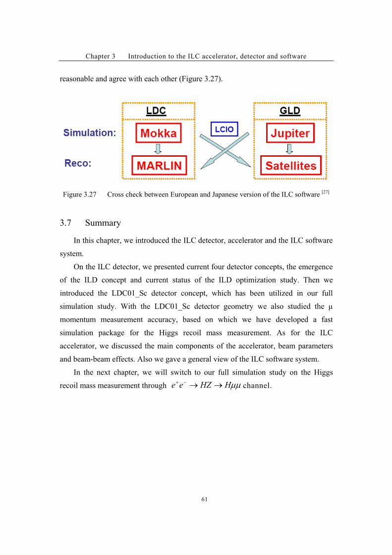
Chapter 3 Introduction to the ILC accelerator, detector and software
61
reasonable and agree with each other (Figure 3.27).
Figure 3.27 Cross check between European and Japanese version of the ILC software [27]
3.7 Summary
In this chapter, we introduced the ILC detector, accelerator and the ILC software
system.
On the ILC detector, we presented current four detector concepts, the emergence
of the ILD concept and current status of the ILD optimization study. Then we
introduced the LDC01_Sc detector concept, which has been utilized in our full
simulation study. With the LDC01_Sc detector geometry we also studied the #
momentum measurement accuracy, based on which we have developed a fast
simulation package for the Higgs recoil mass measurement. As for the ILC
accelerator, we discussed the main components of the accelerator, beam parameters
and beam-beam effects. Also we gave a general view of the ILC software system.
In the next chapter, we will switch to our full simulation study on the Higgs
recoil mass measurement through !!HHZee ""#$channel.
Chapter 4 The Higgs recoil mass and cross section measurement at the ILC
62
Chapter 4 The Higgs recoil mass and cross section
measurement through !!HHZee ""#$ channel
4.1 Introduction
At the ILC most of the Higgs particles will be generated through the
Higgs-strahlung process ( HZee "#$) and the W fusion process ( Hvvee "#$
)[2]
,
see Figure 2.2. For the Higgs-strahlung process, 10 percents of the Z bosons will
decay into a pair of leptons (the chances for each generation of leptons are identical,
about 3.3% each). Because the momentum of #/electron can be precisely measured
by the tracking system, we could measure the recoil mass of the Higgs particle
through the !!HHZee ""#$and HeeHZee ""#$
processes; and,
since when passing through the material the electron has much stronger
radiation effect than the #, we use !!HHZee ""#$process as our signal.
Assume the Higgs mass is 120GeV. The center-of-mass energy is chosen to be
230GeV, about 10% above the product threshold. As shown in Figure 2.3, the cross
section is very close to its maximal at 230GeV center-of-mass energy. Because the
error on Higgs recoil mass is proportional to the muon momentum squared, smaller
center-of-mass energy means better Higgs mass resolution per event [12]
. For non
polarized beam, the cross section for our signal process is about 6.62fb, meaning we
will have about 3310 events with 500fb-1
integrated luminosity.
As we have discussed in Chapter 2.2, here we apply the recoil mass method to
measure the Higgs particle mass. The # momentum could be preciously measured by
the tracking system, take 152 /105/)( ##/0' GeVPPPk 1 , for a 60GeV #, the
momentum measurement accuracy is about 180MeV. With formula 3.1 we can
calculate the expected error on the Higgs recoil mass from the error on #
momentum measurement: assume the Z boson decays into a pair of # with
identical momentum (symmetric case), so GeVpp 5121 00 ; taken
-5
21 10×5 )()( 00 pkpk , then for a single event, the mass measurement accuracy

Chapter 4 The Higgs recoil mass and cross section measurement at the ILC
63
could reach 228MeV; if the Z decays along its momentum direction (the most
asymmetric case), the mass measurement accuracy will be 360MeV per event
– so with totally 3300 events, the accuracy of the Higgs recoil mass
measurement could reach 6MeV level!
The above estimation is obviously too optimistic. First, for # with small polar
angle, the momentum measurement could be much worse than its average level (see
Figure 3.11). While in equation 3.1, we know that the error on Higgs recoil mass
measurement is dominated by the larger error of two # momentum measurements. If
we require both # to be in the “good region” of the detector, i.e., both # with
polar angle bigger than 40 degree, that we will lose almost half of our events.
Second, because of the radiation effect (including beamstrahlung, initial state
radiation (ISR) and final state radiation effect (FSR)), the Higgs recoil mass spectrum
is not a central symmetric distribution: the energy loss caused by any radiation effect
increases the recoil mass, creates a very long high energy tail on the recoil mass
spectrum, see Figure 2.2. Both effects caused the error on the Higgs mass
measurement increased to 30MeV level. In section 4.2 we will discuss in detail the
radiation effect and its effect on the result.
In the recoil mass method we use no information from the Higgs decay final
state. So in principle we could have a model independent Higgs mass measurement
by avoiding using any cut based on Higgs decay final state information (including the
total energy, the multiplicity, the isolation angle, etc). Alternatively, with some
assumptions of the physics model, we could apply some additional cuts to achieve a
better result in the model dependent analysis.
Now we will begin our discussion on radiation effect.
4.2 The Radiation effect
The recoil mass method is very sensitive to the radiation effect. The
beamstrahlung effect (BS) causes the decrease of the center-of-mass energy, while the
# particle loses some of its energy through the ISR and FSR effects. All those three
effects increase the recoil mass, making a high energy tail on the recoil mass
Chapter 4 The Higgs recoil mass and cross section measurement at the ILC
64
spectrum (Figure 2.2). Since the radiation effect is of extremely importance in our
study, we briefly introduce the corresponding simulation tools/method to those effects
and estimate their effect.
As mentioned in Chapter 3, we simulate the Beamstrahlung effect with
Guinea-Pig software, while the output beam file (containing the information of beam
energy with Beamstrahlung effect corrections at the interaction point) is used as the
input file for Pythia and Whizard (Our generator).
The ISR is a very important radiation effect, which can in some case totally
change the physics picture, for example, in !!3"#$ee events (one of our main
background), by radiating a high-energy photon, the ISR effect could reduce
the energy of mediate Z boson to the Z threshold, and make the distribution of
two # invariant mass peak at the Z pole. For the !!HHZee ""#$
process, besides the high energy tail on the recoil mass spectrum, the ISR
effect will affect the cross section, see Figure 2.4. At center-of-mass energy
equal to 230 GeV, the ISR effect will suppress the cross section (according to
the subtraction of phase space) by 20%. Our generator software, Whizard and
Pythia could directly simulate the ISR effect.
Comparing to the ISR effect, the FSR effect is a smaller correction. Also since
the mass of # is about 200 times the electron mass, the FSR effect is much
weak in !!HHZee ""#$ channel than in HeeHZee ""#$
channel.
In our study, the FSR effect is simulated with Pythia (in Whizard the FSR
effect is simulated in the fragmentation step, which is realized by calling
Pythia libraries). We need to mention here that Pythia has not yet considered
the interference between the ISR and FSR effect.
In our analysis, three radiation effects are independently simulated. The
reconstructed recoil mass spectrum could be regarded as a convolution of the
true recoil mass spectrum with the radiation effects and resolution, meaning:
resolutionradiationSpectrueSpecFullSpec ::' )()()( (4.1)
First, let’s study the resolution term in equation 4.1 with our fast
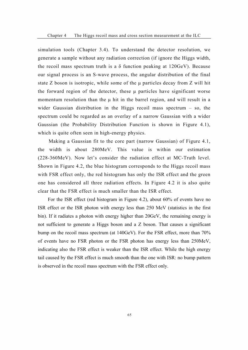
Chapter 4 The Higgs recoil mass and cross section measurement at the ILC
65
simulation tools (Chapter 3.4). To understand the detector resolution, we
generate a sample without any radiation correction (if ignore the Higgs width,
the recoil mass spectrum truth is a & function peaking at 120GeV). Because
our signal process is an S-wave process, the angular distribution of the final
state Z boson is isotropic, while some of the # particles decay from Z will hit
the forward region of the detector, these # particles have significant worse
momentum resolution than the # hit in the barrel region, and will result in a
wider Gaussian distribution in the Higgs recoil mass spectrum – so, the
spectrum could be regarded as an overlay of a narrow Gaussian with a wider
Gaussian (the Probability Distribution Function is shown in Figure 4.1),
which is quite often seen in high-energy physics.
Making a Gaussian fit to the core part (narrow Gaussian) of Figure 4.1,
the width is about 280MeV. This value is within our estimation
(228-360MeV). Now let’s consider the radiation effect at MC-Truth level.
Shown in Figure 4.2, the blue histogram corresponds to the Higgs recoil mass
with FSR effect only, the red histogram has only the ISR effect and the green
one has considered all three radiation effects. In Figure 4.2 it is also quite
clear that the FSR effect is much smaller than the ISR effect.
For the ISR effect (red histogram in Figure 4.2), about 60% of events have no
ISR effect or the ISR photon with energy less than 250 MeV (statistics in the first
bin). If it radiates a photon with energy higher than 20GeV, the remaining energy is
not sufficient to generate a Higgs boson and a Z boson. That causes a significant
bump on the recoil mass spectrum (at 140GeV). For the FSR effect, more than 70%
of events have no FSR photon or the FSR photon has energy less than 250MeV,
indicating also the FSR effect is weaker than the ISR effect. While the high energy
tail caused by the FSR effect is much smooth than the one with ISR: no bump pattern
is observed in the recoil mass spectrum with the FSR effect only.
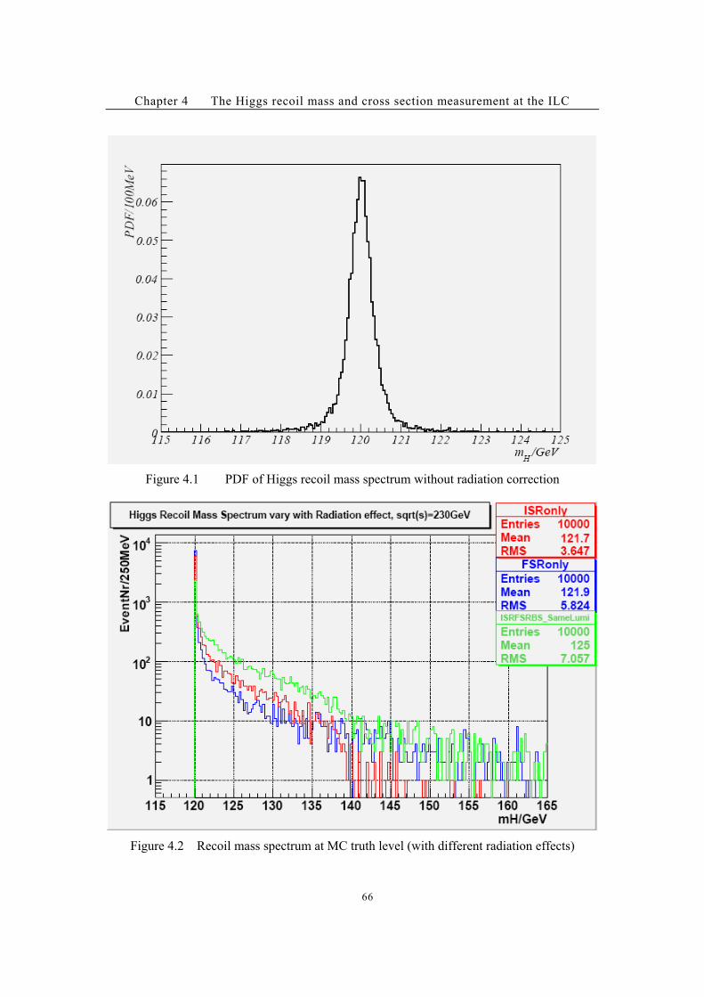
Chapter 4 The Higgs recoil mass and cross section measurement at the ILC
66
Figure 4.1 PDF of Higgs recoil mass spectrum without radiation correction
Figure 4.2 Recoil mass spectrum at MC truth level (with different radiation effects)
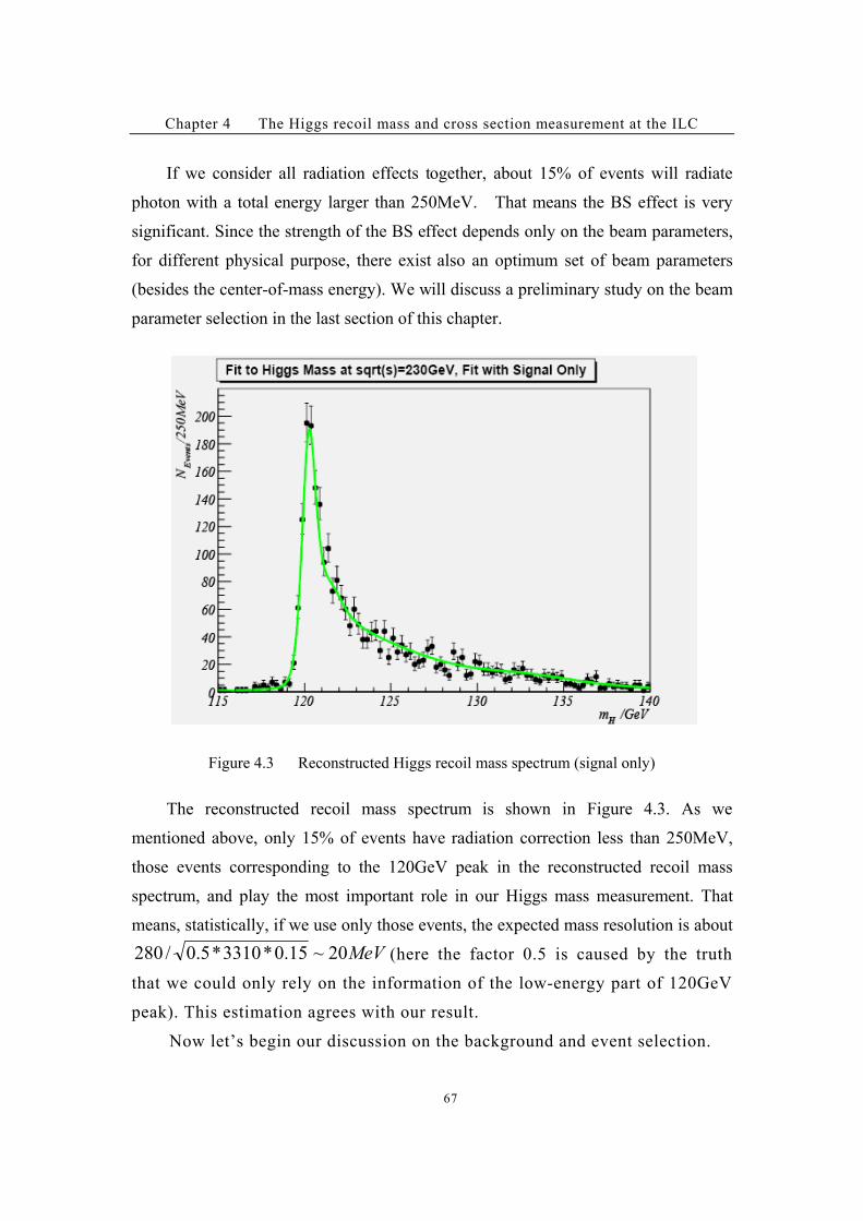
Chapter 4 The Higgs recoil mass and cross section measurement at the ILC
67
If we consider all radiation effects together, about 15% of events will radiate
photon with a total energy larger than 250MeV. That means the BS effect is very
significant. Since the strength of the BS effect depends only on the beam parameters,
for different physical purpose, there exist also an optimum set of beam parameters
(besides the center-of-mass energy). We will discuss a preliminary study on the beam
parameter selection in the last section of this chapter.
Figure 4.3 Reconstructed Higgs recoil mass spectrum (signal only)
The reconstructed recoil mass spectrum is shown in Figure 4.3. As we
mentioned above, only 15% of events have radiation correction less than 250MeV,
those events corresponding to the 120GeV peak in the reconstructed recoil mass
spectrum, and play the most important role in our Higgs mass measurement. That
means, statistically, if we use only those events, the expected mass resolution is about
MeV20~15.0*3310*5.0/280 (here the factor 0.5 is caused by the truth
that we could only rely on the information of the low-energy part of 120GeV
peak). This estimation agrees with our result.
Now let’s begin our discussion on the background and event selection.
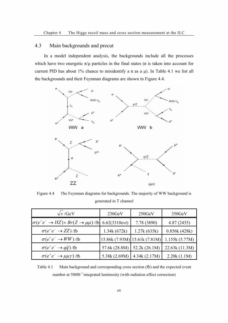
Chapter 4 The Higgs recoil mass and cross section measurement at the ILC
68
4.3 Main backgrounds and precut
In a model independent analysis, the backgrounds include all the processes
which have two energetic %/# particles in the final states (% is taken into account for
current PID has about 1% chance to misidentify a % as a #). In Table 4.1 we list all
the backgrounds and their Feynman diagrams are shown in Figure 4.4.
Figure 4.4 The Feynman diagrams for backgrounds. The majority of WW background is
generated in T channel
s /GeV 230GeV 250GeV 350GeV
)()( !!) "/"#$ ZBrHZee /fb 6.62(3310evt) 7.78 (3890) 4.87 (2435)
)( ZZee "#$) /fb 1.34k (672k) 1.27k (635k) 0.856k (428k)
)( WWee "#$) /fb 15.86k (7.93M) 15.61k (7.81M) 1.155k (5.77M)
)( qqee "#$) /fb 57.6k (28.8M) 52.2k (26.1M) 22.63k (11.3M)
)( !!3) "#$ee /fb 5.38k (2.69M) 4.34k (2.17M) 2.20k (1.1M)
Table 4.1 Main background and corresponding cross section (fb) and the expected event
number at 500fb-1 integrated luminosity (with radiation effect correction)
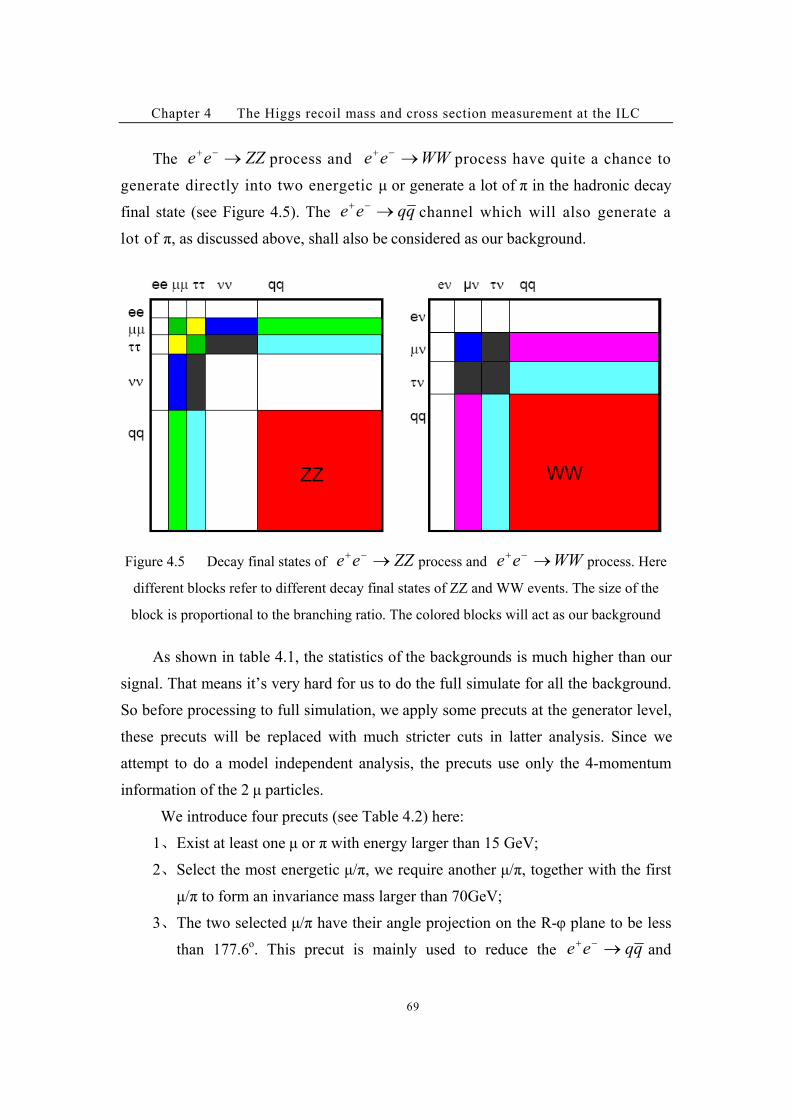
Chapter 4 The Higgs recoil mass and cross section measurement at the ILC
69
The ZZee "#$process and WWee "#$
process have quite a chance to
generate directly into two energetic # or generate a lot of % in the hadronic decay
final state (see Figure 4.5). The qqee "#$channel which will also generate a
lot of %, as discussed above, shall also be considered as our background.
Figure 4.5 Decay final states of ZZee "#$process and WWee "#$
process. Here
different blocks refer to different decay final states of ZZ and WW events. The size of the
block is proportional to the branching ratio. The colored blocks will act as our background
As shown in table 4.1, the statistics of the backgrounds is much higher than our
signal. That means it’s very hard for us to do the full simulate for all the background.
So before processing to full simulation, we apply some precuts at the generator level,
these precuts will be replaced with much stricter cuts in latter analysis. Since we
attempt to do a model independent analysis, the precuts use only the 4-momentum
information of the 2 # particles.
We introduce four precuts (see Table 4.2) here:
1(Exist at least one # or % with energy larger than 15 GeV;
2(Select the most energetic #/%, we require another #/%, together with the first
#/% to form an invariance mass larger than 70GeV;
3(The two selected #/% have their angle projection on the R-+ plane to be less
than 177.6o. This precut is mainly used to reduce the qqee "#$
and
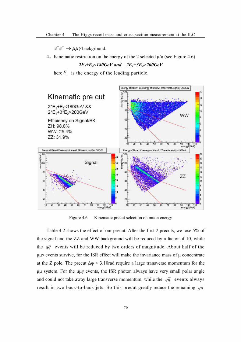
Chapter 4 The Higgs recoil mass and cross section measurement at the ILC
70
!!3"#$ee background.
4(Kinematic restriction on the energy of the 2 selected #/% (see Figure 4.6)
2E1+E2<180GeV and 2E1+3E2>200GeV
here 1E is the energy of the leading particle.
Figure 4.6 Kinematic precut selection on muon energy
Table 4.2 shows the effect of our precut. After the first 2 precuts, we lose 5% of
the signal and the ZZ and WW background will be reduced by a factor of 10, while
the qq events will be reduced by two orders of magnitude. About half of the
##) events survive, for the ISR effect will make the invariance mass of # concentrate
at the Z pole. The precut ,+ < 3.10rad require a large transverse momentum for the
## system. For the ##) events, the ISR photon always have very small polar angle
and could not take away large transverse momentum, while the qq events always
result in two back-to-back jets. So this precut greatly reduce the remaining qq
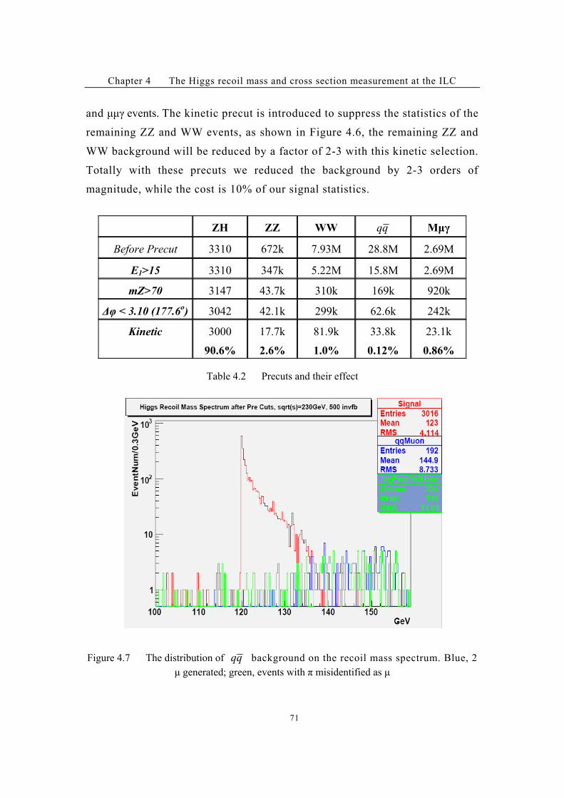
Chapter 4 The Higgs recoil mass and cross section measurement at the ILC
71
and ##) events. The kinetic precut is introduced to suppress the statistics of the
remaining ZZ and WW events, as shown in Figure 4.6, the remaining ZZ and
WW background will be reduced by a factor of 2-3 with this kinetic selection.
Totally with these precuts we reduced the background by 2-3 orders of
magnitude, while the cost is 10% of our signal statistics.
ZH ZZ WW qq !"#
Before Precut 3310 672k 7.93M 28.8M 2.69M
E1>15 3310 347k 5.22M 15.8M 2.69M
mZ>70 3147 43.7k 310k 169k 920k
!" < 3.10 (177.6o) 3042 42.1k 299k 62.6k 242k
Kinetic 3000
90.6%
17.7k
2.6%
81.9k
1.0%
33.8k
0.12%
23.1k
0.86%
Table 4.2 Precuts and their effect
Figure 4.7 The distribution of qq background on the recoil mass spectrum. Blue, 2
# generated; green, events with % misidentified as #
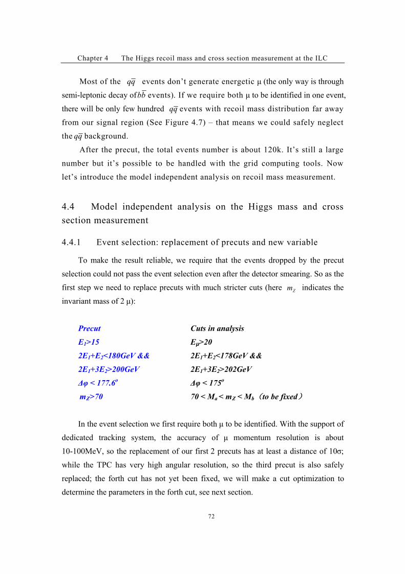
Chapter 4 The Higgs recoil mass and cross section measurement at the ILC
72
Most of the qq events don’t generate energetic # (the only way is through
semi-leptonic decay of bb events). If we require both # to be identified in one event,
there will be only few hundred qq events with recoil mass distribution far away
from our signal region (See Figure 4.7) – that means we could safely neglect
the qq background.
After the precut, the total events number is about 120k. It’s still a large
number but it’s possible to be handled with the grid computing tools. Now
let’s introduce the model independent analysis on recoil mass measurement.
4.4 Model independent analysis on the Higgs mass and cross
section measurement
4.4.1 Event selection: replacement of precuts and new variable
To make the result reliable, we require that the events dropped by the precut
selection could not pass the event selection even after the detector smearing. So as the
first step we need to replace precuts with much stricter cuts (here Zm indicates the
invariant mass of 2 #):
Precut Cuts in analysis
E1>15 E!>20
2E1+E2<180GeV && 2E1+E2<178GeV &&
2E1+3E2>200GeV 2E1+3E2>202GeV
!" < 177.6o !" < 175
o
mZ>70 70 < Ma < mZ < Mb&to be fixed'
In the event selection we first require both # to be identified. With the support of
dedicated tracking system, the accuracy of # momentum resolution is about
10-100MeV, so the replacement of our first 2 precuts has at least a distance of 10*;
while the TPC has very high angular resolution, so the third precut is also safely
replaced; the forth cut has not yet been fixed, we will make a cut optimization to
determine the parameters in the forth cut, see next section.
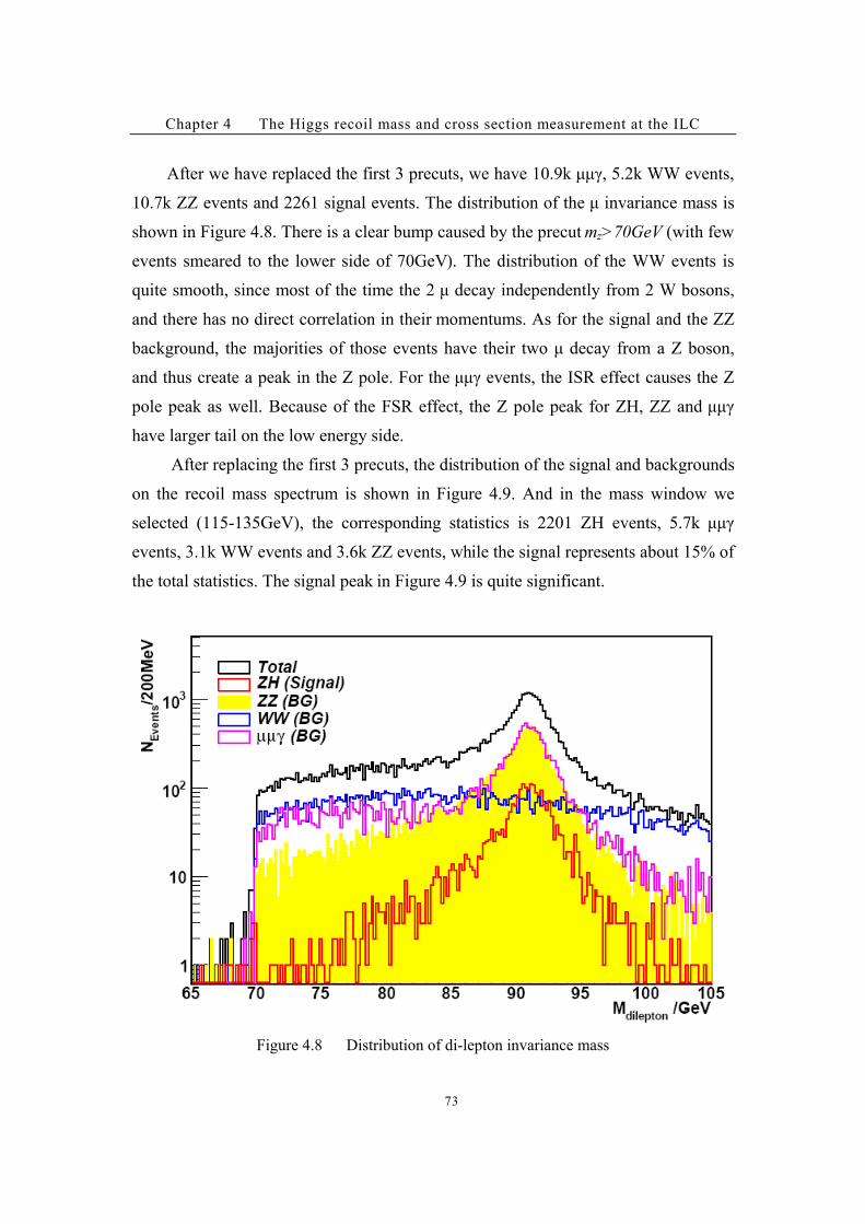
Chapter 4 The Higgs recoil mass and cross section measurement at the ILC
73
After we have replaced the first 3 precuts, we have 10.9k ##), 5.2k WW events,
10.7k ZZ events and 2261 signal events. The distribution of the # invariance mass is
shown in Figure 4.8. There is a clear bump caused by the precut mz>70GeV (with few
events smeared to the lower side of 70GeV). The distribution of the WW events is
quite smooth, since most of the time the 2 # decay independently from 2 W bosons,
and there has no direct correlation in their momentums. As for the signal and the ZZ
background, the majorities of those events have their two # decay from a Z boson,
and thus create a peak in the Z pole. For the ##) events, the ISR effect causes the Z
pole peak as well. Because of the FSR effect, the Z pole peak for ZH, ZZ and ##)
have larger tail on the low energy side.
After replacing the first 3 precuts, the distribution of the signal and backgrounds
on the recoil mass spectrum is shown in Figure 4.9. And in the mass window we
selected (115-135GeV), the corresponding statistics is 2201 ZH events, 5.7k ##)
events, 3.1k WW events and 3.6k ZZ events, while the signal represents about 15% of
the total statistics. The signal peak in Figure 4.9 is quite significant.
Figure 4.8 Distribution of di-lepton invariance mass
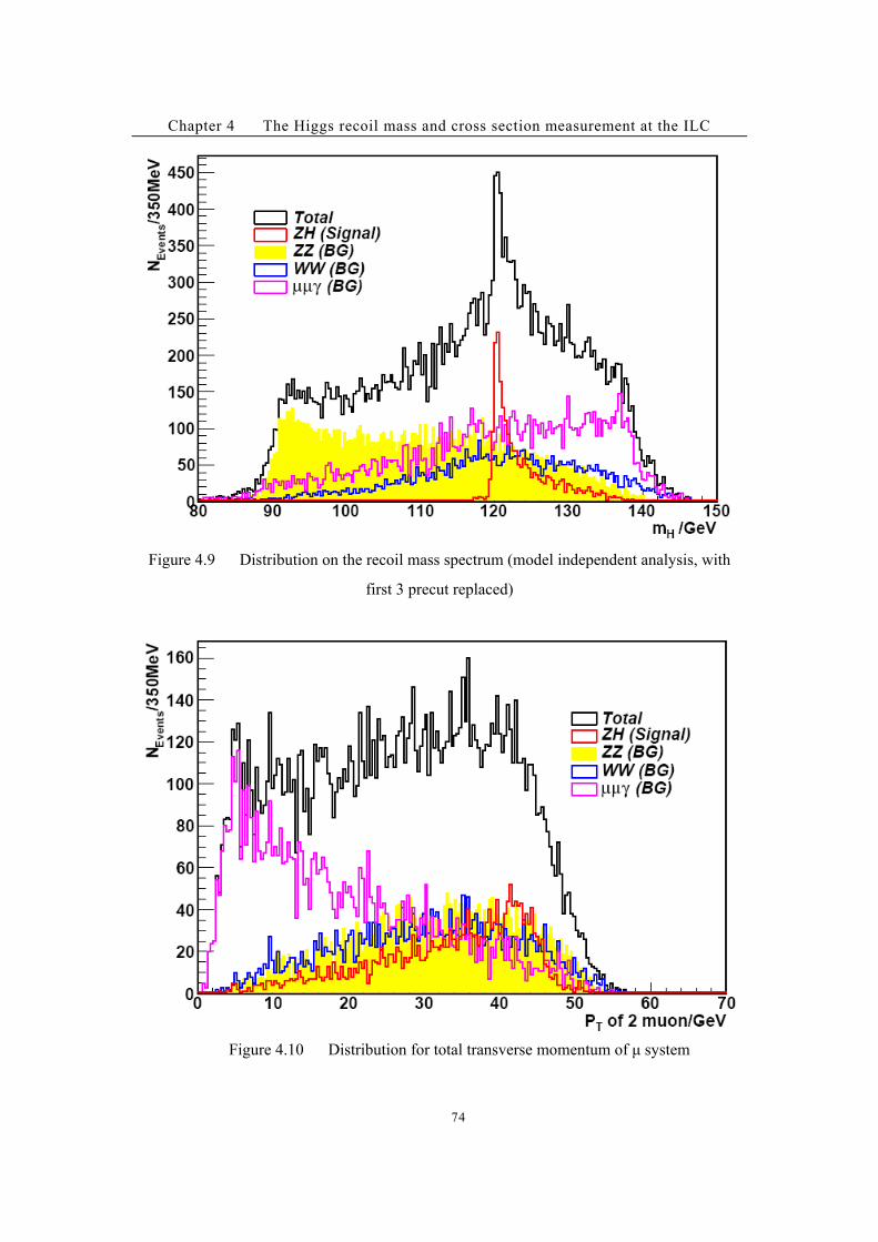
Chapter 4 The Higgs recoil mass and cross section measurement at the ILC
74
Figure 4.9 Distribution on the recoil mass spectrum (model independent analysis, with
first 3 precut replaced)
Figure 4.10 Distribution for total transverse momentum of # system
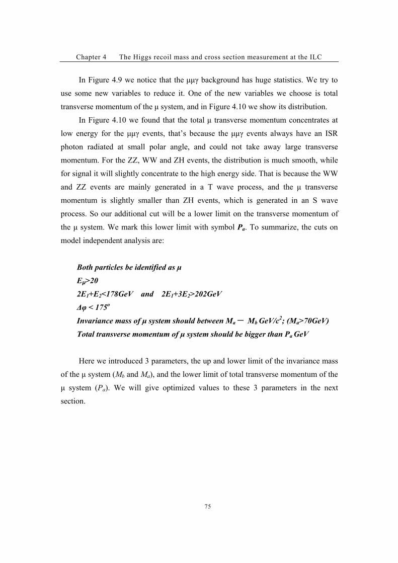
Chapter 4 The Higgs recoil mass and cross section measurement at the ILC
75
In Figure 4.9 we notice that the ##) background has huge statistics. We try to
use some new variables to reduce it. One of the new variables we choose is total
transverse momentum of the # system, and in Figure 4.10 we show its distribution.
In Figure 4.10 we found that the total # transverse momentum concentrates at
low energy for the ##) events, that’s because the ##) events always have an ISR
photon radiated at small polar angle, and could not take away large transverse
momentum. For the ZZ, WW and ZH events, the distribution is much smooth, while
for signal it will slightly concentrate to the high energy side. That is because the WW
and ZZ events are mainly generated in a T wave process, and the # transverse
momentum is slightly smaller than ZH events, which is generated in an S wave
process. So our additional cut will be a lower limit on the transverse momentum of
the # system. We mark this lower limit with symbol Pa. To summarize, the cuts on
model independent analysis are:
Both particles be identified as #
E!>20
2E1+E2<178GeV and 2E1+3E2>202GeV
!" < 175o
Invariance mass of # system should between Ma* Mb GeV/c2; (Ma>70GeV)
Total transverse momentum of # system should be bigger than Pa GeV
Here we introduced 3 parameters, the up and lower limit of the invariance mass
of the # system (Mb and Ma), and the lower limit of total transverse momentum of the
# system (Pa). We will give optimized values to these 3 parameters in the next
section.
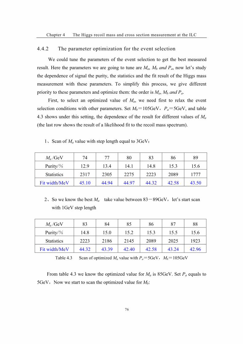
Chapter 4 The Higgs recoil mass and cross section measurement at the ILC
76
4.4.2 The parameter optimization for the event selection
We could tune the parameters of the event selection to get the best measured
result. Here the parameters we are going to tune are Ma, Mb and Pa, now let’s study
the dependence of signal the purity, the statistics and the fit result of the Higgs mass
measurement with these parameters. To simplify this process, we give different
priority to these parameters and optimize them: the order is Ma, Mb and Pa.
First, to select an optimized value of Ma, we need first to relax the event
selection conditions with other parameters. Set Mb)105GeV"Pa)5GeV, and table
4.3 shows under this setting, the dependence of the result for different values of Ma
(the last row shows the result of a likelihood fit to the recoil mass spectrum).
1(Scan of Ma value with step length equal to 3GeV$
Ma /GeV 74 77 80 83 86 89
Purity/+ 12.9 13.4 14.1 14.8 15.3 15.6
Statistics 2317 2305 2275 2223 2089 1777
Fit width/MeV 45.10 44.94 44.97 44.32 42.58 43.50
2(So we know the best Ma take value between 83*89GeV"let’s start scan
with 1GeV step length
Ma /GeV 83 84 85 86 87 88
Purity/+ 14.8 15.0 15.2 15.3 15.5 15.6
Statistics 2223 2186 2145 2089 2025 1923
Fit width/MeV 44.32 43.39 42.40 42.58 43.24 42.96
Table 4.3 Scan of optimized Ma value with Pa)5GeV"Mb)105GeV
From table 4.3 we know the optimized value for Ma is 85GeV. Set Pa equals to
5GeV"Now we start to scan the optimized value for Mb:
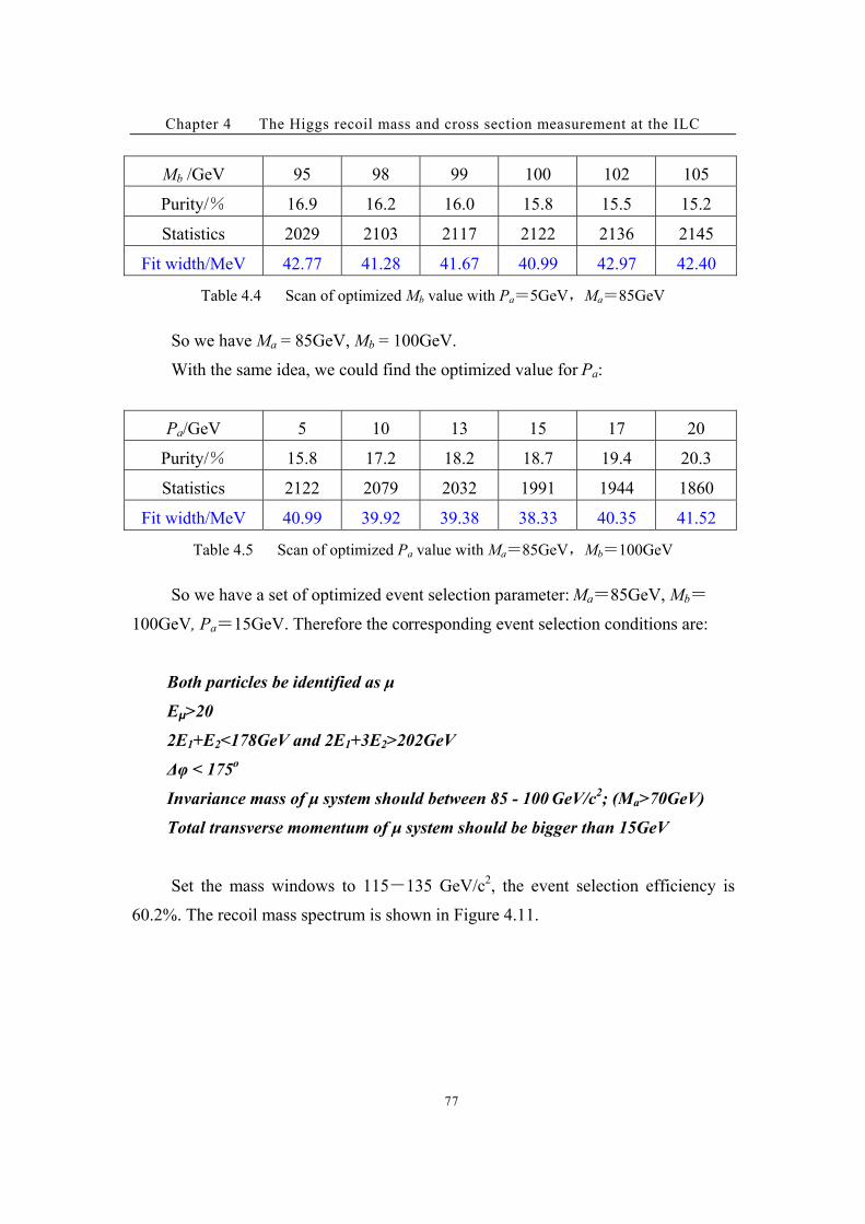
Chapter 4 The Higgs recoil mass and cross section measurement at the ILC
77
Mb /GeV 95 98 99 100 102 105
Purity/+ 16.9 16.2 16.0 15.8 15.5 15.2
Statistics 2029 2103 2117 2122 2136 2145
Fit width/MeV 42.77 41.28 41.67 40.99 42.97 42.40
Table 4.4 Scan of optimized Mb value with Pa)5GeV"Ma)85GeV
So we have Ma = 85GeV, Mb = 100GeV.
With the same idea, we could find the optimized value for Pa:
Pa/GeV 5 10 13 15 17 20
Purity/+ 15.8 17.2 18.2 18.7 19.4 20.3
Statistics 2122 2079 2032 1991 1944 1860
Fit width/MeV 40.99 39.92 39.38 38.33 40.35 41.52
Table 4.5 Scan of optimized Pa value with Ma)85GeV"Mb)100GeV
So we have a set of optimized event selection parameter: Ma)85GeV, Mb)
100GeV, Pa)15GeV. Therefore the corresponding event selection conditions are:
Both particles be identified as #
E!>20
2E1+E2<178GeV and 2E1+3E2>202GeV
!" < 175o
Invariance mass of # system should between 85 - 100 GeV/c2; (Ma>70GeV)
Total transverse momentum of # system should be bigger than 15GeV
Set the mass windows to 115*135 GeV/c2, the event selection efficiency is
60.2%. The recoil mass spectrum is shown in Figure 4.11.
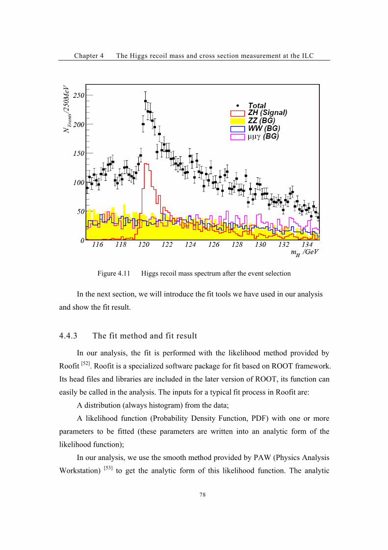
Chapter 4 The Higgs recoil mass and cross section measurement at the ILC
78
Figure 4.11 Higgs recoil mass spectrum after the event selection
In the next section, we will introduce the fit tools we have used in our analysis
and show the fit result.
4.4.3 The fit method and fit result
In our analysis, the fit is performed with the likelihood method provided by
Roofit [52]
. Roofit is a specialized software package for fit based on ROOT framework.
Its head files and libraries are included in the later version of ROOT, its function can
easily be called in the analysis. The inputs for a typical fit process in Roofit are:
A distribution (always histogram) from the data;
A likelihood function (Probability Density Function, PDF) with one or more
parameters to be fitted (these parameters are written into an analytic form of the
likelihood function);
In our analysis, we use the smooth method provided by PAW (Physics Analysis
Workstation) [53]
to get the analytic form of this likelihood function. The analytic
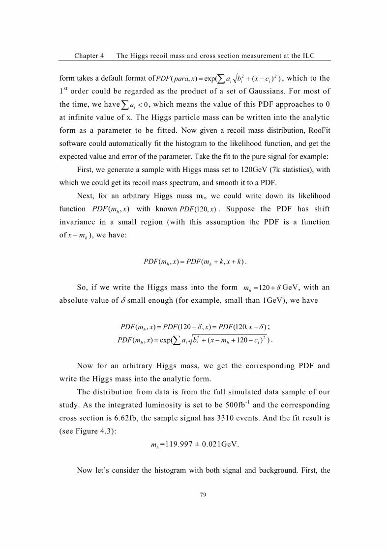
Chapter 4 The Higgs recoil mass and cross section measurement at the ILC
79
form takes a default format of ))(exp(),( 22; #$' iii cxbaxparaPDF , which to the
1st
order could be regarded as the product of a set of Gaussians. For most of
the time, we have 0<; ia , which means the value of this PDF approaches to 0
at infinite value of x. The Higgs particle mass can be written into the analytic
form as a parameter to be fitted. Now given a recoil mass distribution, RooFit
software could automatically fit the histogram to the likelihood function, and get the
expected value and error of the parameter. Take the fit to the pure signal for example:
First, we generate a sample with Higgs mass set to 120GeV (7k statistics), with
which we could get its recoil mass spectrum, and smooth it to a PDF.
Next, for an arbitrary Higgs mass mh, we could write down its likelihood
function ),( xmPDF h with known ),120( xPDF . Suppose the PDF has shift
invariance in a small region (with this assumption the PDF is a function
of hmx # ), we have:
),(),( kxkmPDFxmPDF hh $$' .
So, if we write the Higgs mass into the form 1$'120hm GeV, with an
absolute value of 1 small enough (for example, small than 1GeV), we have
),120(),120(),( 11 #'$' xPDFxPDFxmPDF h;
))120(exp(),( 22; #$#$' ihiih cmxbaxmPDF .
Now for an arbitrary Higgs mass, we get the corresponding PDF and
write the Higgs mass into the analytic form.
The distribution from data is from the full simulated data sample of our
study. As the integrated luminosity is set to be 500fb-1
and the corresponding
cross section is 6.62fb, the sample signal has 3310 events. And the fit result is
(see Figure 4.3):
hm =119.997 ± 0.021GeV.
Now let’s consider the histogram with both signal and background. First, the
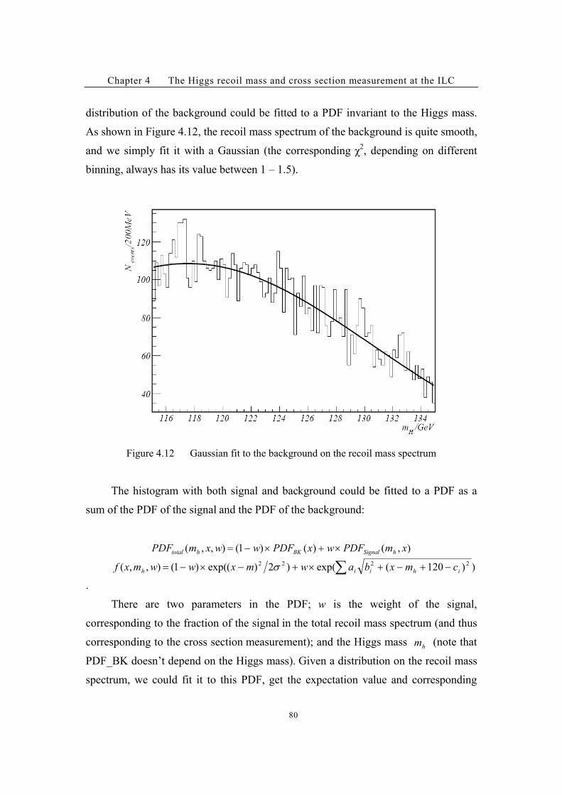
Chapter 4 The Higgs recoil mass and cross section measurement at the ILC
80
distribution of the background could be fitted to a PDF invariant to the Higgs mass.
As shown in Figure 4.12, the recoil mass spectrum of the background is quite smooth,
and we simply fit it with a Gaussian (the corresponding -2, depending on different
binning, always has its value between 1 – 1.5).
Figure 4.12 Gaussian fit to the background on the recoil mass spectrum
The histogram with both signal and background could be fitted to a PDF as a
sum of the PDF of the signal and the PDF of the background:
),()()1(),,( xmPDFwxPDFwwxmPDF hSignalBKhtotal /$/#'
))120(exp()2)(exp()1(),,( 2222 ; #$#$/$#/#' ihiih cmxbawmxwwmxf )
.
There are two parameters in the PDF; w is the weight of the signal,
corresponding to the fraction of the signal in the total recoil mass spectrum (and thus
corresponding to the cross section measurement); and the Higgs mass hm (note that
PDF_BK doesn’t depend on the Higgs mass). Given a distribution on the recoil mass
spectrum, we could fit it to this PDF, get the expectation value and corresponding
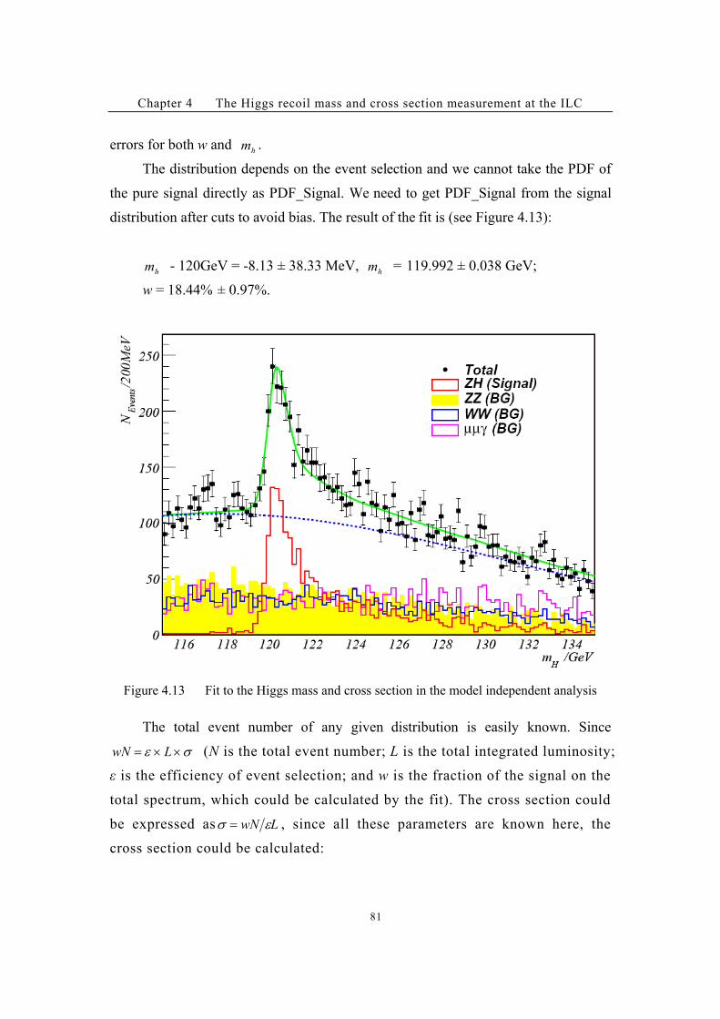
Chapter 4 The Higgs recoil mass and cross section measurement at the ILC
81
errors for both w and hm .
The distribution depends on the event selection and we cannot take the PDF of
the pure signal directly as PDF_Signal. We need to get PDF_Signal from the signal
distribution after cuts to avoid bias. The result of the fit is (see Figure 4.13):
hm - 120GeV = -8.13 ± 38.33 MeV, hm = 119.992 ± 0.038 GeV;
w = 18.44% ± 0.97%.
Figure 4.13 Fit to the Higgs mass and cross section in the model independent analysis
The total event number of any given distribution is easily known. Since
)( //' LwN (N is the total event number; L is the total integrated luminosity;
" is the efficiency of event selection; and w is the fraction of the signal on the
total spectrum, which could be calculated by the fit). The cross section could
be expressed as LwN () ' , since all these parameters are known here, the
cross section could be calculated:
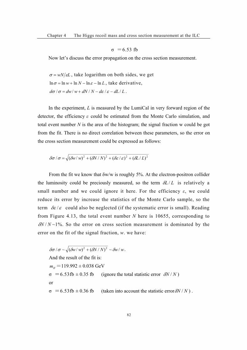
Chapter 4 The Higgs recoil mass and cross section measurement at the ILC
82
* )6.53 fb
Now let’s discuss the error propagation on the cross section measurement.
LwN () ' , take logarithm on both sides, we get
LNw lnlnlnlnln ##$' () , take derivative,
LdLdNdNwdwd ///// ##$' (()) .
In the experiment, L is measured by the LumiCal in very forward region of the
detector, the efficiency " could be estimated from the Monte Carlo simulation, and
total event number N is the area of the histogram; the signal fraction w could be got
from the fit. There is no direct correlation between these parameters, so the error on
the cross section measurement could be expressed as follows:
2222 )/()/()/()/(/ LLNNww 1(1(11)1) $$$'
From the fit we know that &w/w is roughly 5%. At the electron-positron collider
the luminosity could be preciously measured, so the term LL /1 is relatively a
small number and we could ignore it here. For the efficiency ", we could
reduce its error by increase the statistics of the Monte Carlo sample, so the
term (1( / could also be neglected (if the systematic error is small). Reading
from Figure 4.13, the total event number N here is 10655, corresponding to
NN /1 ~1%. So the error on cross section measurement is dominated by the
error on the fit of the signal fraction, w. we have:
wwNNww /~)/()/(~/ 22 111)1) $ .
And the result of the fit is:
Hm )119.992 ± 0.038 GeV
* )6.53fb ± 0.35 fb (ignore the total statistic error NN /1 )
or
* )6.53fb ± 0.36 fb (taken into account the statistic error NN /1 ) .

Chapter 4 The Higgs recoil mass and cross section measurement at the ILC
83
From the above analysis, we found that in the model independent analysis,
Higgs mass could be measured to an accuracy of 38.4MeV, while the relative error on
the cross section measurement could reach 5%. The overall efficiency on event
selection is about 60%. In the next section, we will present the model dependent
measurement.
4.5 The Higgs mass and cross section measurement in model
dependent analysis
4.5.1 Variables used to distinguish event with SM Higgs and
invisible decay Higgs
In different physics models, the behaviors of the Higgs decay are very different.
Setting the Higgs mass equal to 120GeV, the majority of SM Higgs particle will
decay into heavy quark (b, c) pairs or $ lepton pair. While in many other models, the
Higgs could decay invisibly, i.e. the Higgs could decay into a pair of lightest SUSY
particle (LSP) in some SUSY model, or it could decay into a pair of massive
neutrinos. Figure 4.14 shows the comparison of Higgs decay branching ratios in the
SM (right hand side [2]
) and in the model with a massive neutrino (left hand side, the
mass of the 4th
generation of neutrinos is assumed to be 50GeV here [54]
).
On the left plot of Figure 4.14 we found that the majority of Higgs particle will
decay into a pair of 50GeV neutrinos in a wide mass range. We could use two
parameters to distinguish the decay final state of a SM Higgs and an invisible decay
Higgs. They are the total measured energy in one event and the number of tracks with
energy bigger than 3GeV (marked with NTrk). The distribution of these two
parameters for different events is shown in Figure 4.15.
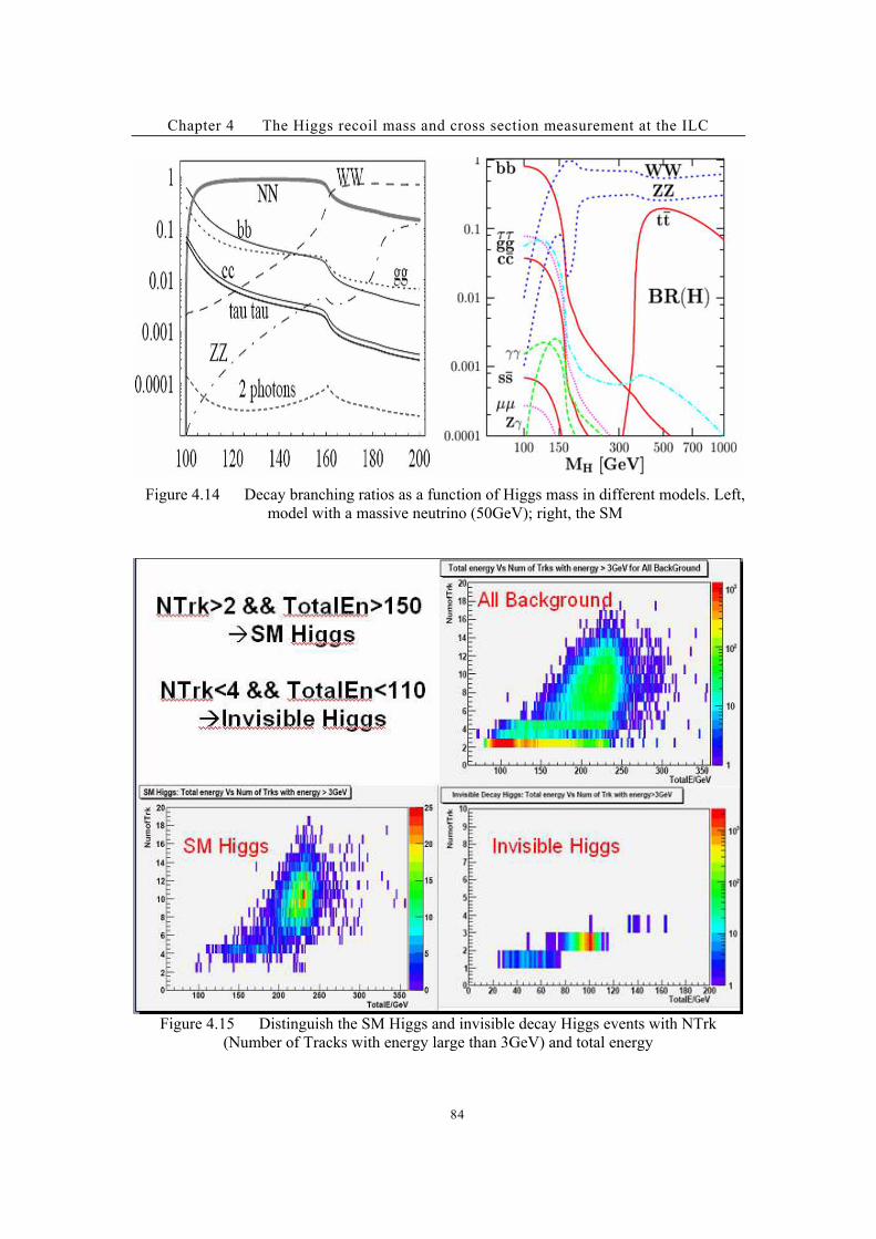
Chapter 4 The Higgs recoil mass and cross section measurement at the ILC
84
Figure 4.14 Decay branching ratios as a function of Higgs mass in different models. Left,
model with a massive neutrino (50GeV); right, the SM
Figure 4.15 Distinguish the SM Higgs and invisible decay Higgs events with NTrk
(Number of Tracks with energy large than 3GeV) and total energy
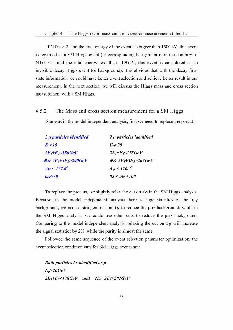
Chapter 4 The Higgs recoil mass and cross section measurement at the ILC
85
If NTrk > 2, and the total energy of the events is bigger than 150GeV, this event
is regarded as a SM Higgs event (or corresponding background); on the contrary, if
NTrk < 4 and the total energy less than 110GeV, this event is considered as an
invisible decay Higgs event (or background). It is obvious that with the decay final
state information we could have better event selection and achieve better result in our
measurement. In the next section, we will discuss the Higgs mass and cross section
measurement with a SM Higgs.
4.5.2 The Mass and cross section measurement for a SM Higgs
Same as in the model independent analysis, first we need to replace the precut:
2 # particles identified 2 # particles identified
E1>15 E!>20
2E1+E2<180GeV 2E1+E2<178GeV
&& 2E1+3E2>200GeV && 2E1+3E2>202GeV
!" < 177.6o !" < 176.4
o
mZ>70 85 < mZ <100
To replace the precuts, we slightly relax the cut on !" in the SM Higgs analysis.
Because, in the model independent analysis there is huge statistics of the ##)
background, we need a stringent cut on !" to reduce the ##) background; while in
the SM Higgs analysis, we could use other cuts to reduce the ##) background.
Comparing to the model independent analysis, relaxing the cut on !" will increase
the signal statistics by 2%, while the purity is almost the same.
Followed the same sequence of the event selection parameter optimization, the
event selection condition cuts for SM Higgs events are:
Both particles be identified as #
E!>20GeV
2E1+E2<178GeV and 2E1+3E2>202GeV
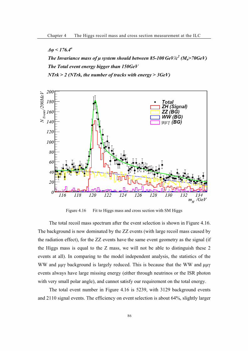
Chapter 4 The Higgs recoil mass and cross section measurement at the ILC
86
!" < 176.4o
The Invariance mass of # system should between 85-100 GeV/c2 (Ma>70GeV)
The Total event energy bigger than 150GeV
NTrk > 2 (NTrk, the number of tracks with energy > 3GeV)
Figure 4.16 Fit to Higgs mass and cross section with SM Higgs
The total recoil mass spectrum after the event selection is shown in Figure 4.16.
The background is now dominated by the ZZ events (with large recoil mass caused by
the radiation effect), for the ZZ events have the same event geometry as the signal (if
the Higgs mass is equal to the Z mass, we will not be able to distinguish these 2
events at all). In comparing to the model independent analysis, the statistics of the
WW and ##) background is largely reduced. This is because that the WW and ##)
events always have large missing energy (either through neutrinos or the ISR photon
with very small polar angle), and cannot satisfy our requirement on the total energy.
The total event number in Figure 4.16 is 5239, with 3129 background events
and 2110 signal events. The efficiency on event selection is about 64%, slightly larger
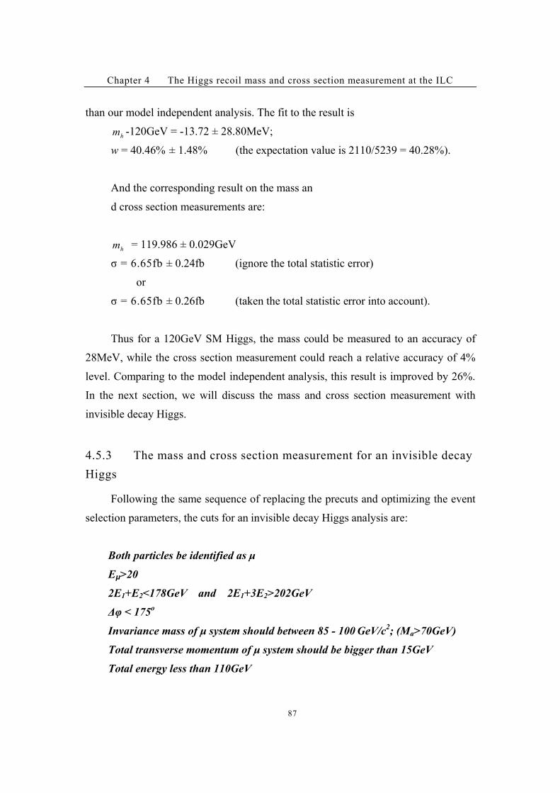
Chapter 4 The Higgs recoil mass and cross section measurement at the ILC
87
than our model independent analysis. The fit to the result is
hm -120GeV = -13.72 ± 28.80MeV;
w = 40.46% ± 1.48% (the expectation value is 2110/5239 = 40.28%).
And the corresponding result on the mass an
d cross section measurements are:
hm = 119.986 ± 0.029GeV
* = 6.65fb ± 0.24fb (ignore the total statistic error)
or
* = 6.65fb ± 0.26fb (taken the total statistic error into account).
Thus for a 120GeV SM Higgs, the mass could be measured to an accuracy of
28MeV, while the cross section measurement could reach a relative accuracy of 4%
level. Comparing to the model independent analysis, this result is improved by 26%.
In the next section, we will discuss the mass and cross section measurement with
invisible decay Higgs.
4.5.3 The mass and cross section measurement for an invisible decay
Higgs
Following the same sequence of replacing the precuts and optimizing the event
selection parameters, the cuts for an invisible decay Higgs analysis are:
Both particles be identified as #
E!>20
2E1+E2<178GeV and 2E1+3E2>202GeV
!" < 175o
Invariance mass of # system should between 85 - 100 GeV/c2; (Ma>70GeV)
Total transverse momentum of # system should be bigger than 15GeV
Total energy less than 110GeV
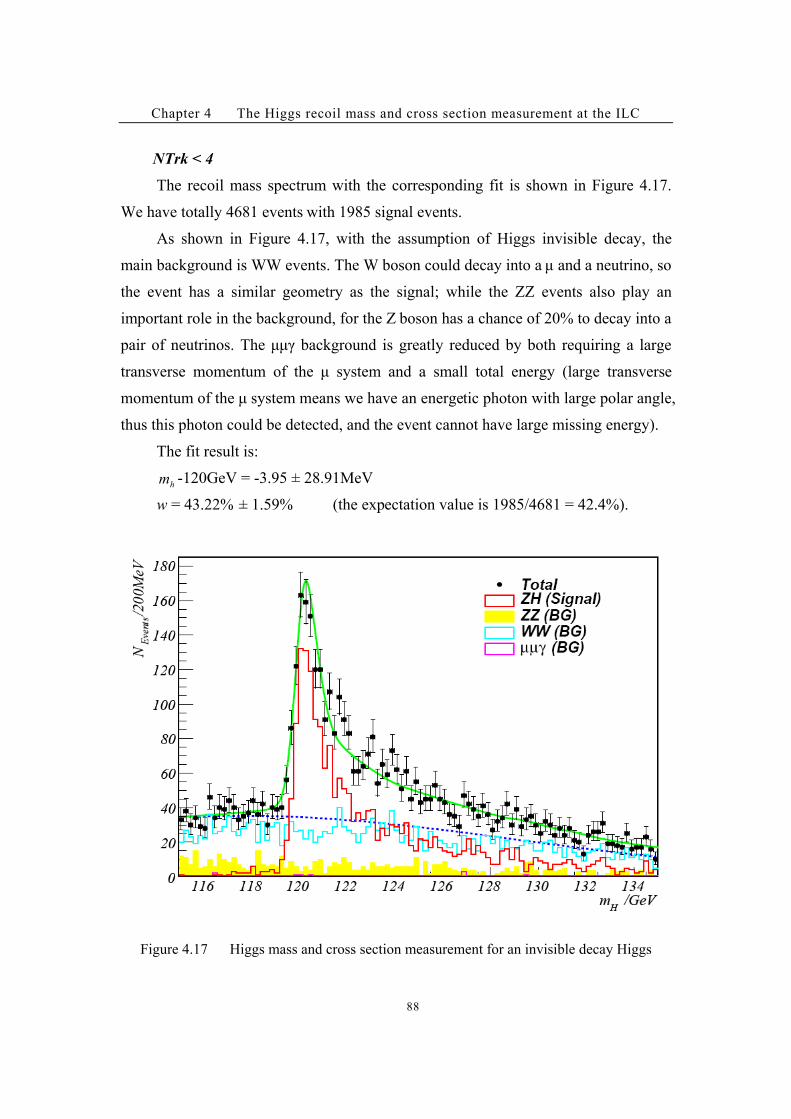
Chapter 4 The Higgs recoil mass and cross section measurement at the ILC
88
NTrk < 4
The recoil mass spectrum with the corresponding fit is shown in Figure 4.17.
We have totally 4681 events with 1985 signal events.
As shown in Figure 4.17, with the assumption of Higgs invisible decay, the
main background is WW events. The W boson could decay into a # and a neutrino, so
the event has a similar geometry as the signal; while the ZZ events also play an
important role in the background, for the Z boson has a chance of 20% to decay into a
pair of neutrinos. The ##) background is greatly reduced by both requiring a large
transverse momentum of the # system and a small total energy (large transverse
momentum of the # system means we have an energetic photon with large polar angle,
thus this photon could be detected, and the event cannot have large missing energy).
The fit result is:
hm -120GeV = -3.95 ± 28.91MeV
w = 43.22% ± 1.59% (the expectation value is 1985/4681 = 42.4%).
Figure 4.17 Higgs mass and cross section measurement for an invisible decay Higgs

Chapter 4 The Higgs recoil mass and cross section measurement at the ILC
89
And the corresponding results on the mass and cross section measurements are:
hm = 119.996 ± 0.029GeV
* = 6.80fb ± 0.25fb (ignore the total statistic error)
or
* = 6.80fb ± 0.27fb (taken the total statistic error into account)
The result of the Higgs invisible decay analysis is comparable with the SM
Higgs analysis. The accuracy of the Higgs mass measurement is 29MeV, and the
relative error on the cross section measurement is 4%.
In the next section we will switch to the preliminary study of the beam
parameter optimization/selection: let’s consider the Higgs mass measurement in terms
of machine parameters.
4.6 Preliminary study on the beam parameter optimization
Same as the detector optimization study, there exist a set of optimized beam
parameters for different physical observable measurement, with which we could
achieve better measurement performance and less machine time at the same time.
Our starting point for the beam parameter is the nominal beam parameter at
500GeV center-of-mass energy. As for the beam parameter optimization for Higgs
recoil mass measurement (which might work at 230GeV center-of-mass energy as
discussed in previous chapter), first, let’s consider two different beam parameter
selections.
First, keep the basic beam parameters (#z $x $y) constant for different
center-of-mass energy. With this method, the luminosity is proportional to the
centre-of-mass energy, while the BS effect is proportional to the square of
center-of-mass energy. Thus, when we lower the center-of-mass energy from
500GeV to 230GeV, we will roughly have half of the luminosity with the
same machine time (actually even less for at small center-of-mass energy we
suffer more from the wake field luminosity reduction) and less than one

Chapter 4 The Higgs recoil mass and cross section measurement at the ILC
90
quarter of the beamstrahlung effect.
Second, we can scale our beam parameters with the center-of-mass
energy. This method will provide us the same luminosity and the same
strength of the beamstrahlung effect as for the 500GeV nominal beam. This is
the method we have used in our full simulation study, which needs really
strong Final Focusing (FF) system.
Of course there exist some other choices in between. Table 4.6 [55]
are
sets of the beam parameters the Beam Delivery System (BDS) group purposed.
Their suggestion is much closer to the first method and relatively more
realistic with our current technique.
There are eight sets of beam parameters in the BDS group proposal,
including three center-of-mass energy (230GeV, 250GeV and 350GeV) and
two sets of L*, which is the distance of the FF solenoid to the interaction
point. With smaller L* the FF system could provide more powerful focus and
result in larger luminosity, but the disadvantage is that we might need to
install the FF system inside the detector. The CollX is also an important
parameter, which is also called the field depth of the FF system. CollX<6 is
regarded as a current technique limit for the FF system. .L is the parameter we
used to describe the wake field reduction of the luminosity, it increases with
center-of-mass energy. The luminosity marked with the bold character is the
luminosity we could achieve with the same machine time for us to achieve
500fb-1
integrated luminosity for the 500GeV nominal beam. And the last line
of Table 4.6 (marked with blue character) is the fit result of the fast
simulation (see chapter 3.4.2).
Chapter 4 The Higgs recoil mass and cross section measurement at the ILC
91
Sqrt(s)/GeV 230 230 250 250 350 350 350 350
L* /m 3.5 4.5 3.5 4.5 3.5 4.5 3.5 4.5
/x /mm 22.7 29.2 20.9 26.9 15.0 19.2 20.3 20.5
ColliX 6 6 6 6 6 6 7.0 6.2
.L /% 80.7 77.0 83.0 79.5 90.1 87.8 90.1 87.8
L/1037
m-2
s-1
6.70 5.55 7.93 6.54 14.7 12.4 12.4 12.1
L /fb-1
181 150 214 177 397 335 335 327
*(H!!)/fb 7.03 7.06 7.81 7.83 4.80 4.80 4.78 4.80
N_events 1272 1059 1671 1386 1906 1608 1601 1570
&(mH)/MeV 19.5 21.4 23.3 25.7 78.8 89.5 84.5 83.8
Table 4.6 Beam parameters purposed by the BDS group and the expected Higgs
mass measurement accuracy [55]
By loading the beam parameters to the Guinea-Pig software package and
using its output beam file as the input file for our generator, we could
calculate the true value of corresponding recoil mass with all the radiation
effect correction. Then, with the fast simulation package, by convoluting the
true value of the Higgs recoil mass spectrum to the detector resolution, we get
the expected recoil mass spectrum after reconstruction (See Figure 4.18, 4.19),
and with a likelihood fit we can get the expectation value and expected
measurement error on the Higgs mass.
The last line of Table 4.6 shows the expected error on the Higgs mass
measurement for each set of beam parameters. When we ignore all the background,
and assume the detector has a signal efficiency to 100%, we can achieve the best
Higgs mass measurement at 230GeV, L*=3.5 meter. The corresponding mass
measurement error is 19.5 MeV.
Interestingly, this 19.5MeV accuracy is comparable with the fit result to pure
signal in our full simulation study, where we adopt the second method of beam
parameter selection. Though for the latter case, we have much higher luminosity.
That’s because with the beam parameter purposed by the BDS group we have much

Chapter 4 The Higgs recoil mass and cross section measurement at the ILC
92
less beamstrahlung effect, and thus the events are much more concentrated to the
main peak, which plays the most important role in Higgs mass measurement. Of
course, with a comparable mass measurement accuracy and comparable cost, the
method with higher luminosity is more attractive for we have more Higgs particles
there – which will be important for the measurement of other Higgs particle
properties.
And actually when we lower the center-of-mass energy, we have other methods
to increase the luminosity. For example, we could increase the number of
electron/positrons in the bunch, or increase the bunch number or frequency, etc. This
is quite interesting and needs further study.
The beam parameter optimization, as well as the detector optimization study is
very important and very complex. There are many possibilities and chances for us to
achieve better physics result. For example, we could performance the same beam
optimization study with fine energy bins. The optimization on beam parameters and
detector parameters are the two closely related subjects, with only carefully
considering together we could achieve the best performance.
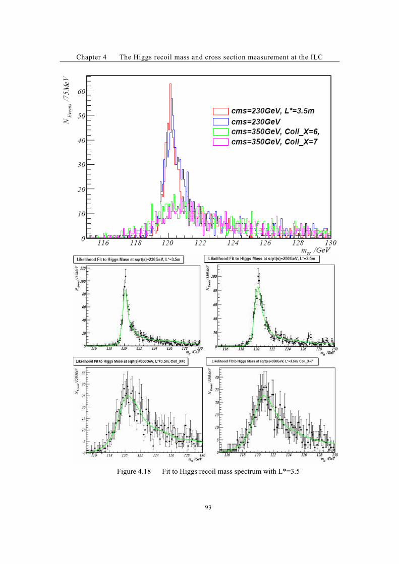
Chapter 4 The Higgs recoil mass and cross section measurement at the ILC
93
Figure 4.18 Fit to Higgs recoil mass spectrum with L*=3.5
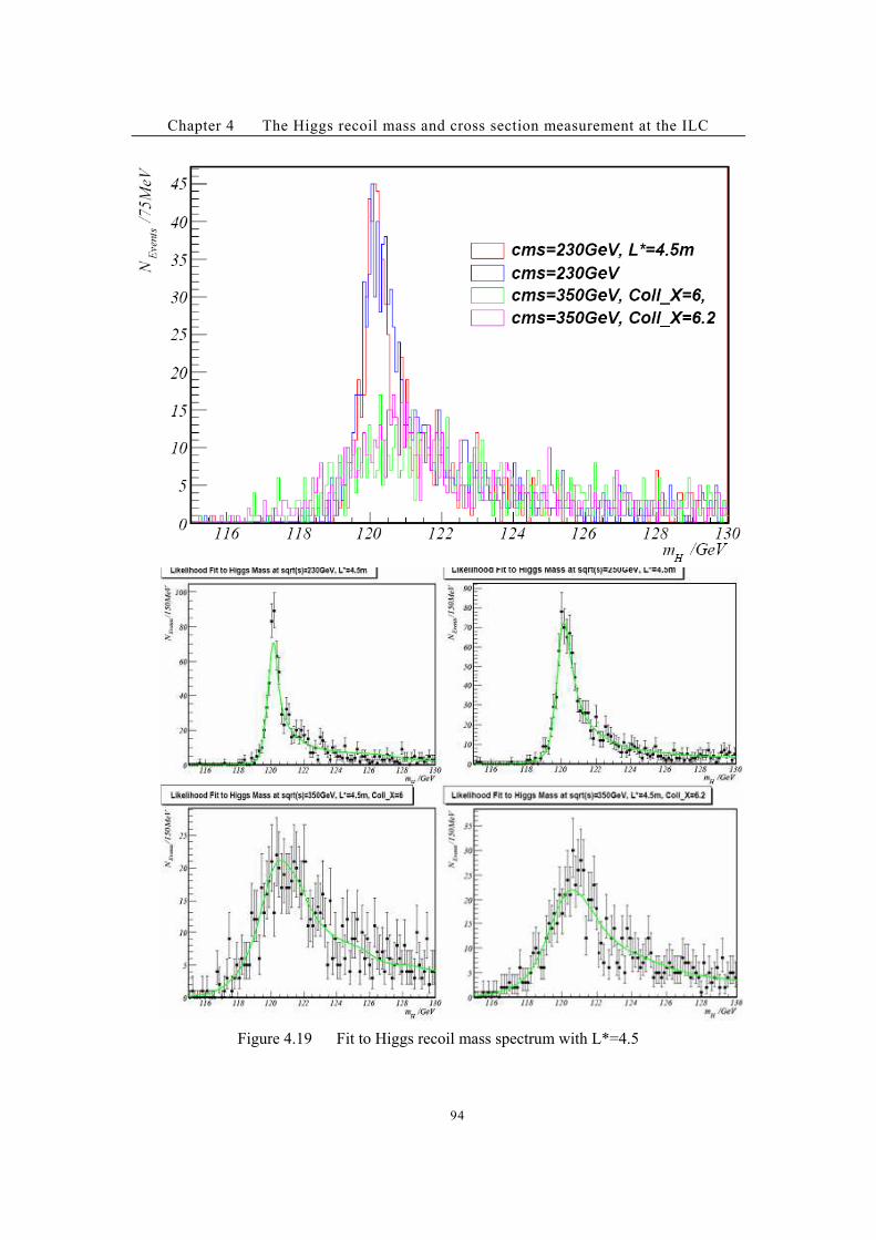
Chapter 4 The Higgs recoil mass and cross section measurement at the ILC
94
Figure 4.19 Fit to Higgs recoil mass spectrum with L*=4.5
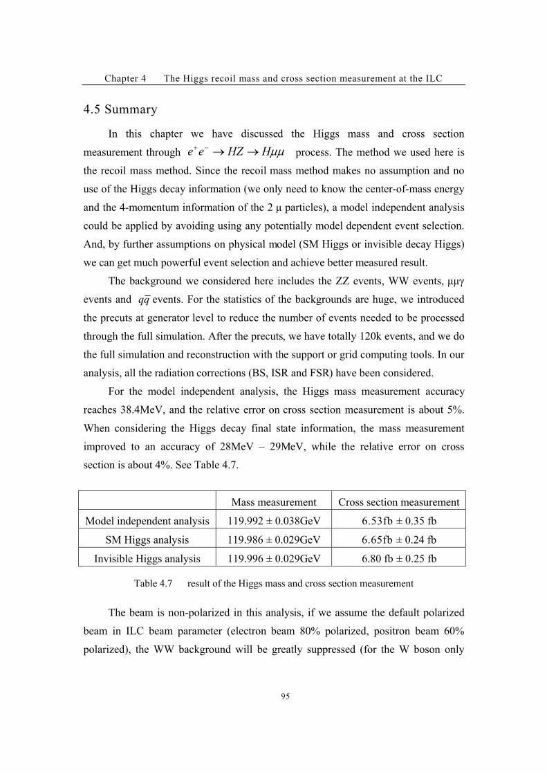
Chapter 4 The Higgs recoil mass and cross section measurement at the ILC
95
4.5 Summary
In this chapter we have discussed the Higgs mass and cross section
measurement through !!HHZee ""#$ process. The method we used here is
the recoil mass method. Since the recoil mass method makes no assumption and no
use of the Higgs decay information (we only need to know the center-of-mass energy
and the 4-momentum information of the 2 # particles), a model independent analysis
could be applied by avoiding using any potentially model dependent event selection.
And, by further assumptions on physical model (SM Higgs or invisible decay Higgs)
we can get much powerful event selection and achieve better measured result.
The background we considered here includes the ZZ events, WW events, ##)
events and qq events. For the statistics of the backgrounds are huge, we introduced
the precuts at generator level to reduce the number of events needed to be processed
through the full simulation. After the precuts, we have totally 120k events, and we do
the full simulation and reconstruction with the support or grid computing tools. In our
analysis, all the radiation corrections (BS, ISR and FSR) have been considered.
For the model independent analysis, the Higgs mass measurement accuracy
reaches 38.4MeV, and the relative error on cross section measurement is about 5%.
When considering the Higgs decay final state information, the mass measurement
improved to an accuracy of 28MeV – 29MeV, while the relative error on cross
section is about 4%. See Table 4.7.
Mass measurement Cross section measurement
Model independent analysis 119.992 ± 0.038GeV 6.53fb ± 0.35 fb
SM Higgs analysis 119.986 ± 0.029GeV 6.65fb ± 0.24 fb
Invisible Higgs analysis 119.996 ± 0.029GeV 6.80 fb ± 0.25 fb
Table 4.7 result of the Higgs mass and cross section measurement
The beam is non-polarized in this analysis, if we assume the default polarized
beam in ILC beam parameter (electron beam 80% polarized, positron beam 60%
polarized), the WW background will be greatly suppressed (for the W boson only
Chapter 4 The Higgs recoil mass and cross section measurement at the ILC
96
couples to left-handed electron), and the statistics of our signal could increase by 58%
(in the SM the coupling of the Z boson to left hand and right hand electrons are not
the same due to the parity violation of weak interaction. The effect of the beam
polarization on the signal cross section could be seen in Figure 2.4). As for the
detector concept, we use the minimal LDC detector concept (LDC01_Sc), with
smaller TPC, minimal silicon tracker (only has VTX and 2-layer SIT, no SET or ETD
in between the TPC and ECAL) and no # tracker installed in the YOKE. So our result
is expected to improve a lot by using a more complete detector and the polarized
beams.
Based on the knowledge of the beam effect we introduced in Chapter 3.5.2, a
preliminary study on the beam parameter optimization for the Higgs recoil mass
measurement has been carried out with beam parameters proposed by the BDS group.
Same as for the detector optimization study, the beam parameter optimization study
for different physical purposes is very important. The analysis is done at fast
simulation level with the package developed by ourselves. In all the eight sets of
proposed beam parameters, the best Higgs mass measurement is achieved with
230GeV center-of-mass energy and 3.5m L* (L* is the distance between interaction
point to the FF system). This conclusion also supports our choice of 230GeV
center-of-mass energy in our full simulation study (in comparing to 250GeV or
350GeV center-of-mass energy).
So far we have finished our discussion on the Higgs mass measurement study
with Monte Carlo simulation, in the next chapter we are going to discuss the CALICE
test beam experiment and its data analysis.
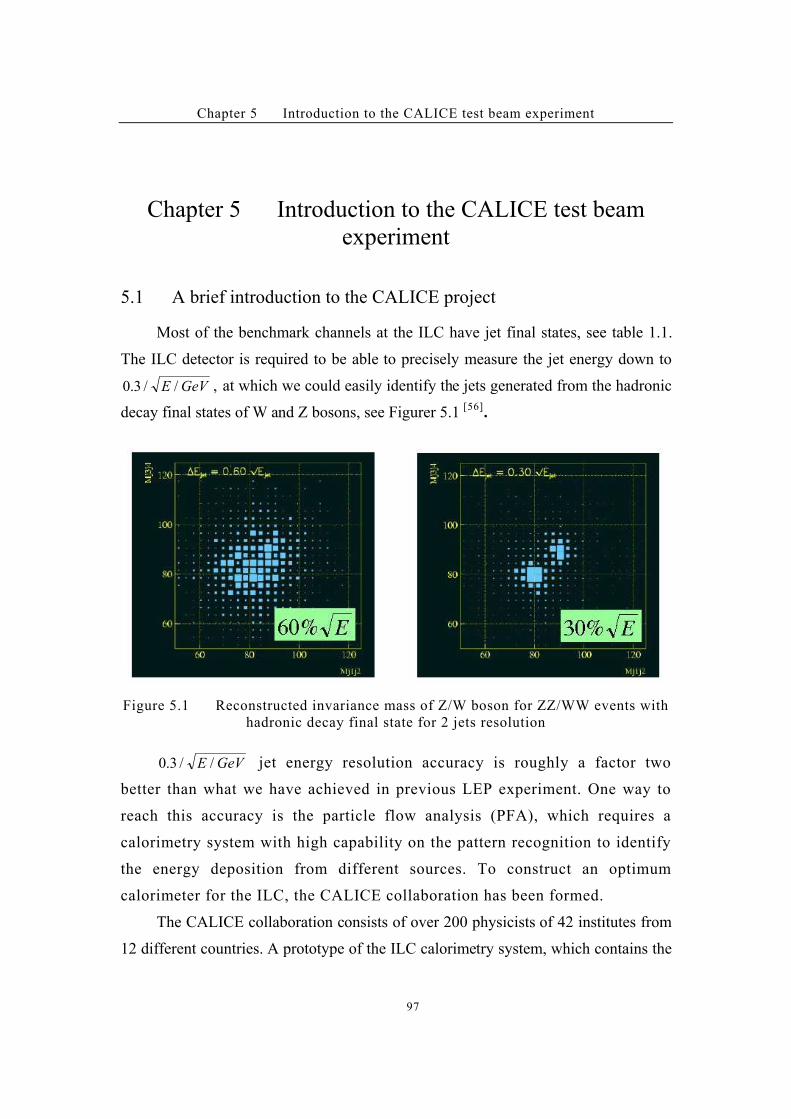
Chapter 5 Introduction to the CALICE test beam experiment
97
Chapter 5 Introduction to the CALICE test beam
experiment
5.1 A brief introduction to the CALICE project
Most of the benchmark channels at the ILC have jet final states, see table 1.1.
The ILC detector is required to be able to precisely measure the jet energy down to
GeVE //3.0 , at which we could easily identify the jets generated from the hadronic
decay final states of W and Z bosons, see Figurer 5.1 [56]
.
Figure 5.1 Reconstructed invariance mass of Z/W boson for ZZ/WW events with
hadronic decay final state for 2 jets resolution
GeVE //3.0 jet energy resolution accuracy is roughly a factor two
better than what we have achieved in previous LEP experiment. One way to
reach this accuracy is the particle flow analysis (PFA), which requires a
calorimetry system with high capability on the pattern recognition to identify
the energy deposition from different sources. To construct an optimum
calorimeter for the ILC, the CALICE collaboration has been formed.
The CALICE collaboration consists of over 200 physicists of 42 institutes from
12 different countries. A prototype of the ILC calorimetry system, which contains the
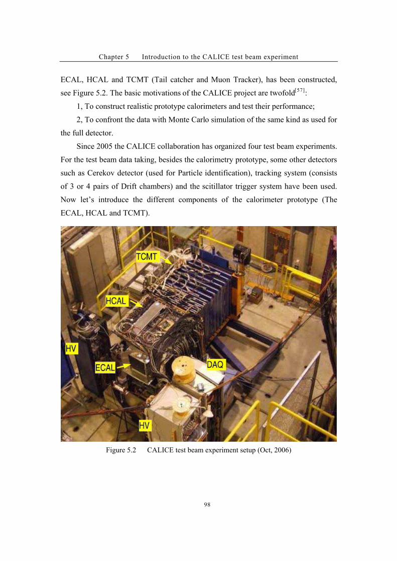
Chapter 5 Introduction to the CALICE test beam experiment
98
ECAL, HCAL and TCMT (Tail catcher and Muon Tracker), has been constructed,
see Figure 5.2. The basic motivations of the CALICE project are twofold[57]
:
1, To construct realistic prototype calorimeters and test their performance;
2, To confront the data with Monte Carlo simulation of the same kind as used for
the full detector.
Since 2005 the CALICE collaboration has organized four test beam experiments.
For the test beam data taking, besides the calorimetry prototype, some other detectors
such as Cerekov detector (used for Particle identification), tracking system (consists
of 3 or 4 pairs of Drift chambers) and the scitillator trigger system have been used.
Now let’s introduce the different components of the calorimeter prototype (The
ECAL, HCAL and TCMT).
Figure 5.2 CALICE test beam experiment setup (Oct, 2006)
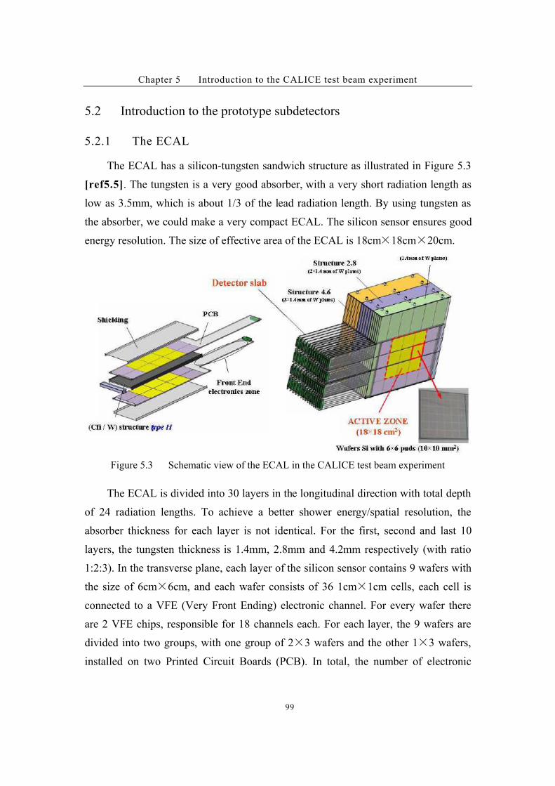
Chapter 5 Introduction to the CALICE test beam experiment
99
5.2 Introduction to the prototype subdetectors
5.2.1 The ECAL!
The ECAL has a silicon-tungsten sandwich structure as illustrated in Figure 5.3
[ref5.5]. The tungsten is a very good absorber, with a very short radiation length as
low as 3.5mm, which is about 1/3 of the lead radiation length. By using tungsten as
the absorber, we could make a very compact ECAL. The silicon sensor ensures good
energy resolution. The size of effective area of the ECAL is 18cm#18cm#20cm.
Figure 5.3 Schematic view of the ECAL in the CALICE test beam experiment
The ECAL is divided into 30 layers in the longitudinal direction with total depth
of 24 radiation lengths. To achieve a better shower energy/spatial resolution, the
absorber thickness for each layer is not identical. For the first, second and last 10
layers, the tungsten thickness is 1.4mm, 2.8mm and 4.2mm respectively (with ratio
1:2:3). In the transverse plane, each layer of the silicon sensor contains 9 wafers with
the size of 6cm#6cm, and each wafer consists of 36 1cm#1cm cells, each cell is
connected to a VFE (Very Front Ending) electronic channel. For every wafer there
are 2 VFE chips, responsible for 18 channels each. For each layer, the 9 wafers are
divided into two groups, with one group of 2#3 wafers and the other 1#3 wafers,
installed on two Printed Circuit Boards (PCB). In total, the number of electronic
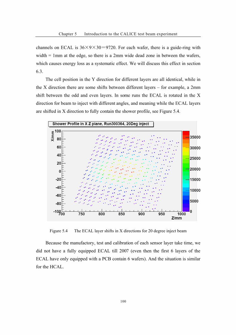
Chapter 5 Introduction to the CALICE test beam experiment
100
channels on ECAL is 36#9#30)9720. For each wafer, there is a guide-ring with
width = 1mm at the edge, so there is a 2mm wide dead zone in between the wafers,
which causes energy loss as a systematic effect. We will discuss this effect in section
6.3.
The cell position in the Y direction for different layers are all identical, while in
the X direction there are some shifts between different layers – for example, a 2mm
shift between the odd and even layers. In some runs the ECAL is rotated in the X
direction for beam to inject with different angles, and meaning while the ECAL layers
are shifted in X direction to fully contain the shower profile, see Figure 5.4.
Figure 5.4 The ECAL layer shifts in X directions for 20 degree inject beam
Because the manufactory, test and calibration of each sensor layer take time, we
did not have a fully equipped ECAL till 2007 (even then the first 6 layers of the
ECAL have only equipped with a PCB contain 6 wafers). And the situation is similar
for the HCAL.
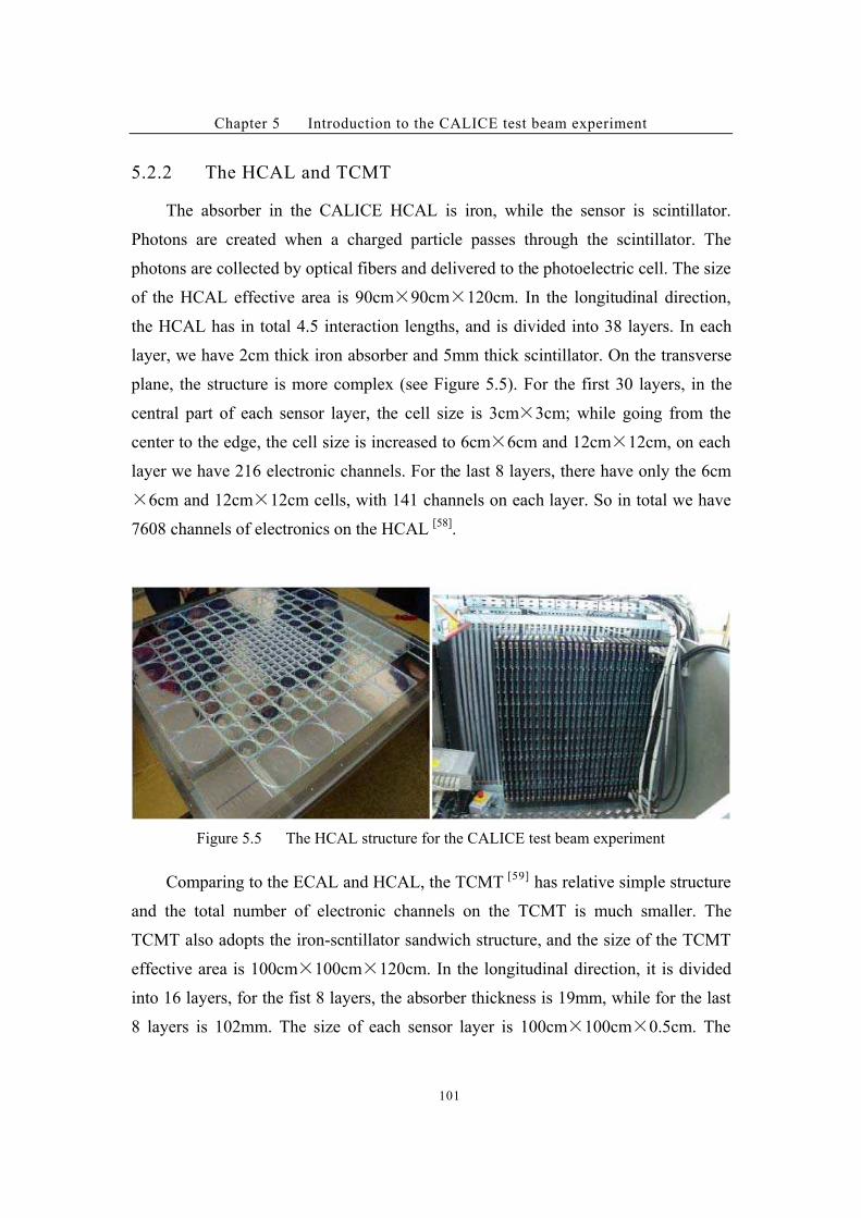
Chapter 5 Introduction to the CALICE test beam experiment
101
5.2.2 The HCAL and TCMT!
The absorber in the CALICE HCAL is iron, while the sensor is scintillator.
Photons are created when a charged particle passes through the scintillator. The
photons are collected by optical fibers and delivered to the photoelectric cell. The size
of the HCAL effective area is 90cm#90cm#120cm. In the longitudinal direction,
the HCAL has in total 4.5 interaction lengths, and is divided into 38 layers. In each
layer, we have 2cm thick iron absorber and 5mm thick scintillator. On the transverse
plane, the structure is more complex (see Figure 5.5). For the first 30 layers, in the
central part of each sensor layer, the cell size is 3cm#3cm; while going from the
center to the edge, the cell size is increased to 6cm#6cm and 12cm#12cm, on each
layer we have 216 electronic channels. For the last 8 layers, there have only the 6cm
#6cm and 12cm#12cm cells, with 141 channels on each layer. So in total we have
7608 channels of electronics on the HCAL [58]
.
Figure 5.5 The HCAL structure for the CALICE test beam experiment
Comparing to the ECAL and HCAL, the TCMT [59]
has relative simple structure
and the total number of electronic channels on the TCMT is much smaller. The
TCMT also adopts the iron-scntillator sandwich structure, and the size of the TCMT
effective area is 100cm#100cm#120cm. In the longitudinal direction, it is divided
into 16 layers, for the fist 8 layers, the absorber thickness is 19mm, while for the last
8 layers is 102mm. The size of each sensor layer is 100cm#100cm#0.5cm. The
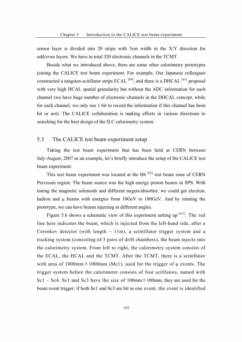
Chapter 5 Introduction to the CALICE test beam experiment
102
sensor layer is divided into 20 strips with 5cm width in the X/Y direction for
odd/even layers. We have in total 320 electronic channels in the TCMT.
Beside what we introduced above, there are some other calorimetry prototypes
joining the CALICE test beam experiment. For example, Our Japanese colleagues
constructed a tungsten-scitillator strips ECAL [60]
, and there is a DHCAL [61]
proposal
with very high HCAL spatial granularity but without the ADC information for each
channel (we have huge number of electronic channels in the DHCAL concept, while
for each channel, we only use 1 bit to record the information if this channel has been
hit or not). The CALICE collaboration is making efforts in various directions to
searching for the best design of the ILC calorimetry system.
5.3 The CALICE test beam experiment setup
Taking the test beam experiment that has been held at CERN between
July-August, 2007 as an example, let’s briefly introduce the setup of the CALICE test
beam experiment.
This test beam experiment was located at the H6 [62]
test beam zone of CERN
Prevessin region. The beam source was the high energy proton beams in SPS. With
tuning the magnetic solenoids and different targets/absorber, we could get electron,
hadron and # beams with energies from 10GeV to 180GeV. And by rotating the
prototype, we can have beams injecting at different angles.
Figure 5.6 shows a schematic view of this experiment setting up [63]
. The red
line here indicates the beam, which is injected from the left-hand side, after a
Cerenkov detector (with length ~ 11m), a scintillator trigger system and a
tracking system (consisting of 3 pairs of drift chambers), the beam injects into
the calorimetry system. From left to right, the calorimetry system consists of
the ECAL, the HCAL and the TCMT. After the TCMT, there is a scintllator
with area of 1000mm#1000mm (Mc1), used for the trigger of # events. The
trigger system before the calorimeter consists of four scitllators, named with
Sc1 – Sc4. Sc1 and Sc3 have the size of 100mm#100mm, they are used for the
beam event trigger: if both Sc1 and Sc3 are hit in one event, the event is identified
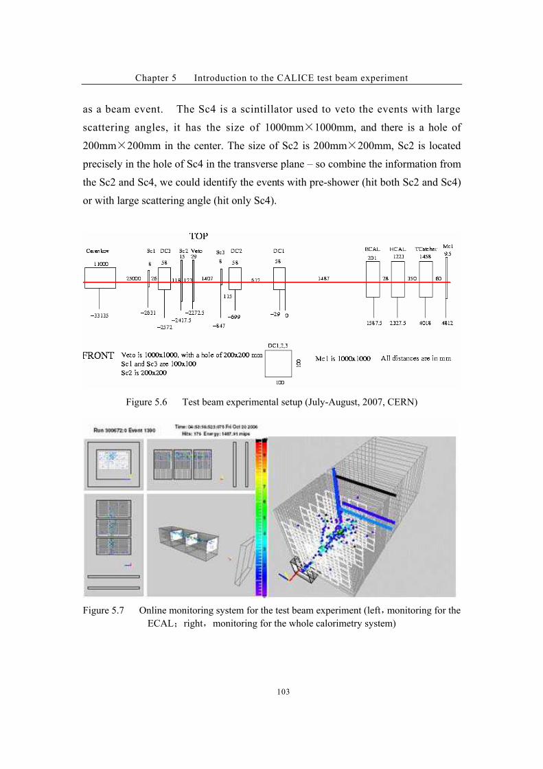
Chapter 5 Introduction to the CALICE test beam experiment
103
as a beam event. The Sc4 is a scintillator used to veto the events with large
scattering angles, it has the size of 1000mm#1000mm, and there is a hole of
200mm#200mm in the center. The size of Sc2 is 200mm#200mm, Sc2 is located
precisely in the hole of Sc4 in the transverse plane – so combine the information from
the Sc2 and Sc4, we could identify the events with pre-shower (hit both Sc2 and Sc4)
or with large scattering angle (hit only Sc4).
'
Figure 5.6 Test beam experimental setup (July-August, 2007, CERN)
Figure 5.7 Online monitoring system for the test beam experiment (left"monitoring for the
ECAL%right"monitoring for the whole calorimetry system)
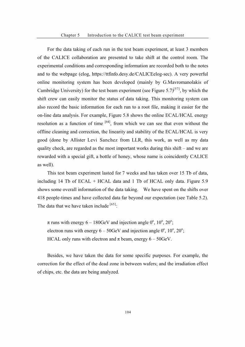
Chapter 5 Introduction to the CALICE test beam experiment
104
For the data taking of each run in the test beam experiment, at least 3 members
of the CALICE collaboration are presented to take shift at the control room. The
experimental conditions and corresponding information are recorded both to the notes
and to the webpage (elog, https://ttfinfo.desy.de/CALICEelog-sec). A very powerful
online monitoring system has been developed (mainly by G.Mavromanolakis of
Cambridge University) for the test beam experiment (see Figure 5.7)[57]
, by which the
shift crew can easily monitor the status of data taking. This monitoring system can
also record the basic information for each run to a root file, making it easier for the
on-line data analysis. For example, Figure 5.8 shows the online ECAL/HCAL energy
resolution as a function of time [64]
, from which we can see that even without the
offline cleaning and correction, the linearity and stability of the ECAL/HCAL is very
good (done by Allister Levi Sanchez from LLR, this work, as well as my data
quality check, are regarded as the most important works during this shift – and we are
rewarded with a special gift, a bottle of honey, whose name is coincidently CALICE
as well).
This test beam experiment lasted for 7 weeks and has taken over 15 Tb of data,
including 14 Tb of ECAL + HCAL data and 1 Tb of HCAL only data. Figure 5.9
shows some overall information of the data taking. We have spent on the shifts over
418 people-times and have collected data far beyond our expectation (see Table 5.2).
The data that we have taken include [65]
:
% runs with energy 6 – 180GeV and injection angle 0o, 10
o, 20
o;
electron runs with energy 6 – 50GeV and injection angle 0o, 10
o, 20
o;
HCAL only runs with electron and % beam, energy 6 – 50GeV.
Besides, we have taken the data for some specific purposes. For example, the
correction for the effect of the dead zone in between wafers; and the irradiation effect
of chips, etc. the data are being analyzed.
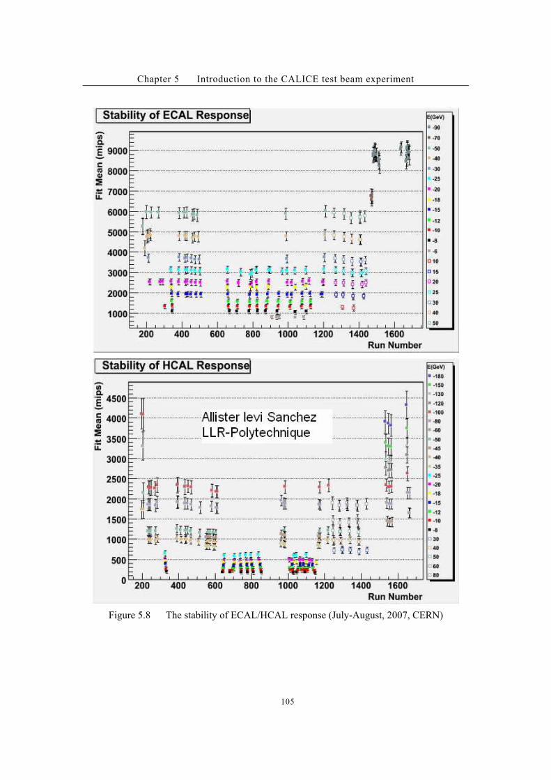
Chapter 5 Introduction to the CALICE test beam experiment
105
Figure 5.8 The stability of ECAL/HCAL response (July-August, 2007, CERN)
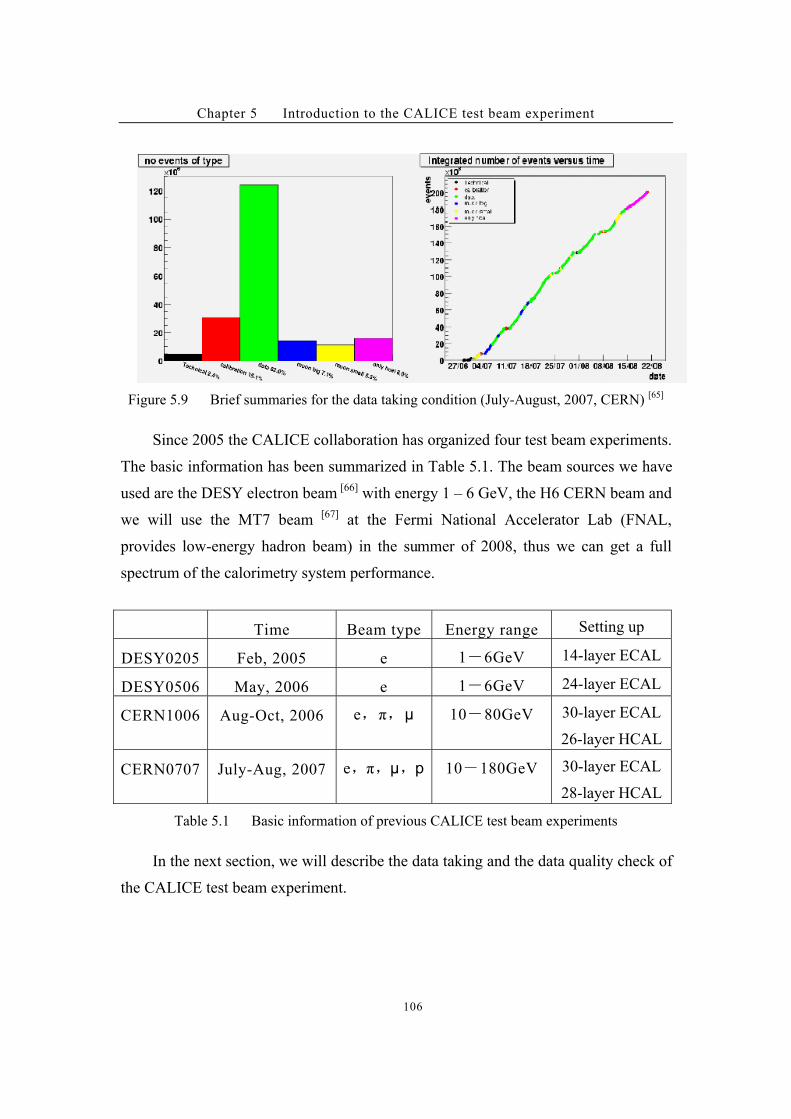
Chapter 5 Introduction to the CALICE test beam experiment
106
Figure 5.9 Brief summaries for the data taking condition (July-August, 2007, CERN) [65]
Since 2005 the CALICE collaboration has organized four test beam experiments.
The basic information has been summarized in Table 5.1. The beam sources we have
used are the DESY electron beam [66]
with energy 1 – 6 GeV, the H6 CERN beam and
we will use the MT7 beam [67]
at the Fermi National Accelerator Lab (FNAL,
provides low-energy hadron beam) in the summer of 2008, thus we can get a full
spectrum of the calorimetry system performance.
Time Beam type Energy range Setting up
DESY0205 Feb, 2005 e 1*6GeV 14-layer ECAL
DESY0506 May, 2006 e 1*6GeV 24-layer ECAL
CERN1006 Aug-Oct, 2006 e"%"! 10*80GeV 30-layer ECAL
26-layer HCAL
CERN0707 July-Aug, 2007 e"%"!"p 10*180GeV 30-layer ECAL
28-layer HCAL
Table 5.1 Basic information of previous CALICE test beam experiments
In the next section, we will describe the data taking and the data quality check of
the CALICE test beam experiment.
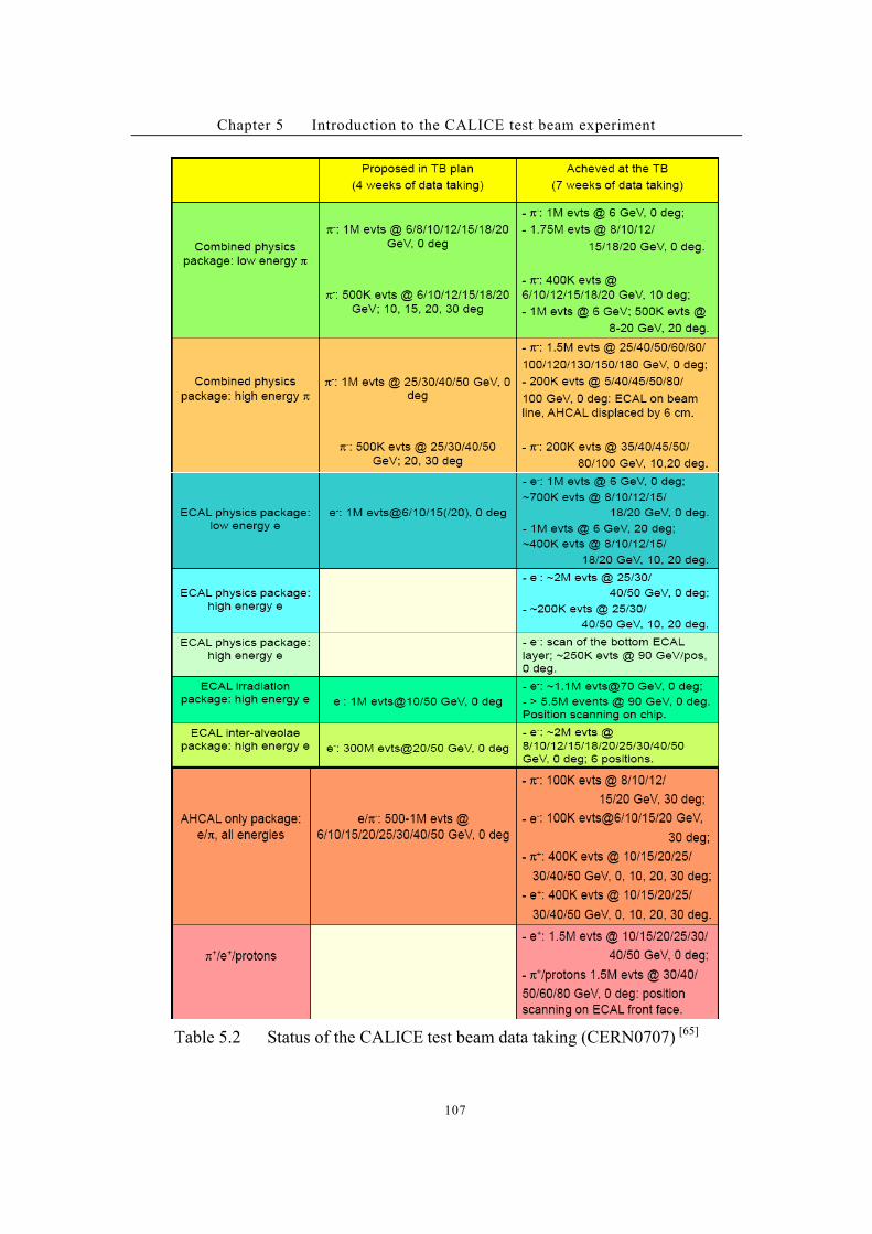
Chapter 5 Introduction to the CALICE test beam experiment
107
Table 5.2 Status of the CALICE test beam data taking (CERN0707) [65]
Chapter 5 Introduction to the CALICE test beam experiment
108
5.4 The data acquisition and data flow of the CALICE test beam
experiment
In the test beam experiment, the data acquisition system first writes the
electronic signal from the detector to a binary file. The binary files (divided into 2 GB
in size each) were first stored in a hard-disk cluster in the control room, and at the
same time the data format transformation and reconstruction through the grid
computing is processed.
The binary files are first transformed into the standard format of slcio
files. The latter files contain the ADC value of each channel and some global
run parameters. After the pedestal subtraction and calibration, the information
is reconstructed into calorimeter hits. The data (the binary file, the
transformed slcio file and the reconstructed file) are transported to the grid
storing elements and any member of the CALICE collaboration could access
these data files through the CALICE Virtual Organization (VO).
5.4.1 The ECAL Calibration!
The calibration constant for each ECAL channel is obtained from the cosmic ray
experiments and the # events data in the test beam experiment (while for the on-line
monitoring and analysis, we use calibration constants calculated from previous data).
After the pedestal subtraction, a hit with more than 25 ADC values is regarded as an
effective hit. Since 1 mip is about 50 ADC value, this condition is about 0.5 mip cut.
The following conditions are used for the # event selection[57]
;
First, the number of effective hits should between 15 and 40 (totally 30 layers);
Second, the projection of these hits on the transverse plane should be within 2
cm distance on both directions.
In total we have collected over 10M # events in CERN 2007 test beam
experiment.
For a single ECAL cell, the distribution of energy deposition of a # event could
be regarded as a Gaussian distribution convolute with a Landau distribution, see
Figure 5.10. The most probable value of this distribution is defined as the calibration
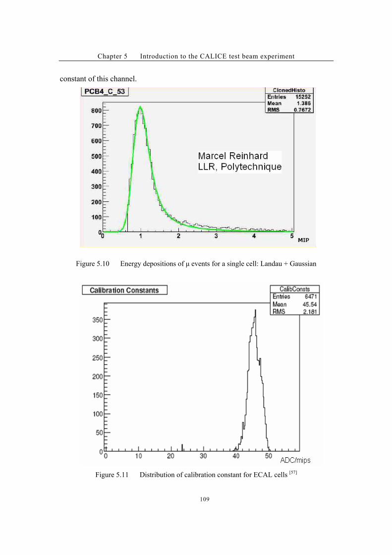
Chapter 5 Introduction to the CALICE test beam experiment
109
constant of this channel.
Figure 5.10 Energy depositions of # events for a single cell: Landau + Gaussian
Figure 5.11 Distribution of calibration constant for ECAL cells [57]
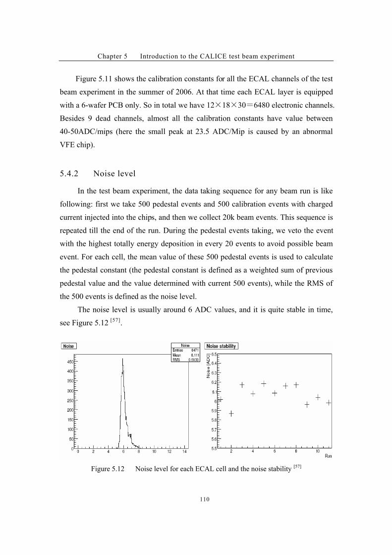
Chapter 5 Introduction to the CALICE test beam experiment
110
Figure 5.11 shows the calibration constants for all the ECAL channels of the test
beam experiment in the summer of 2006. At that time each ECAL layer is equipped
with a 6-wafer PCB only. So in total we have 12#18#30)6480 electronic channels.
Besides 9 dead channels, almost all the calibration constants have value between
40-50ADC/mips (here the small peak at 23.5 ADC/Mip is caused by an abnormal
VFE chip).
5.4.2 Noise level !
In the test beam experiment, the data taking sequence for any beam run is like
following: first we take 500 pedestal events and 500 calibration events with charged
current injected into the chips, and then we collect 20k beam events. This sequence is
repeated till the end of the run. During the pedestal events taking, we veto the event
with the highest totally energy deposition in every 20 events to avoid possible beam
event. For each cell, the mean value of these 500 pedestal events is used to calculate
the pedestal constant (the pedestal constant is defined as a weighted sum of previous
pedestal value and the value determined with current 500 events), while the RMS of
the 500 events is defined as the noise level.
The noise level is usually around 6 ADC values, and it is quite stable in time,
see Figure 5.12 [57]
.
Figure 5.12 Noise level for each ECAL cell and the noise stability [57]
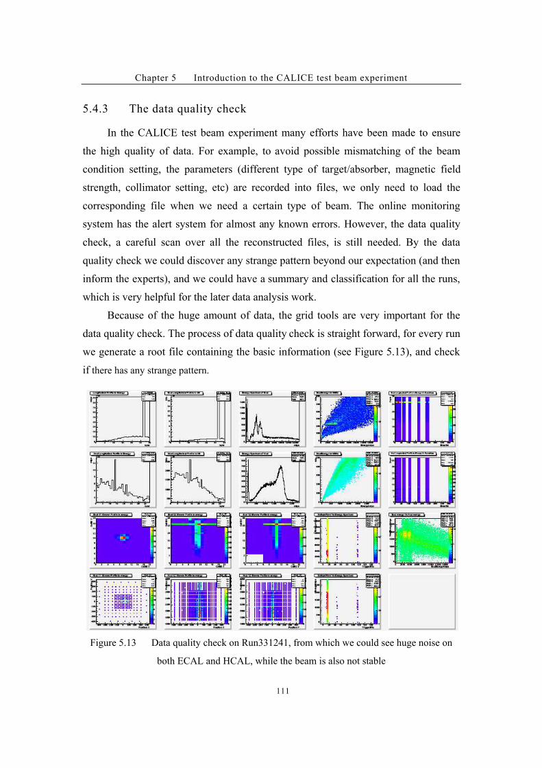
Chapter 5 Introduction to the CALICE test beam experiment
111
5.4.3 The data quality check!
In the CALICE test beam experiment many efforts have been made to ensure
the high quality of data. For example, to avoid possible mismatching of the beam
condition setting, the parameters (different type of target/absorber, magnetic field
strength, collimator setting, etc) are recorded into files, we only need to load the
corresponding file when we need a certain type of beam. The online monitoring
system has the alert system for almost any known errors. However, the data quality
check, a careful scan over all the reconstructed files, is still needed. By the data
quality check we could discover any strange pattern beyond our expectation (and then
inform the experts), and we could have a summary and classification for all the runs,
which is very helpful for the later data analysis work.
Because of the huge amount of data, the grid tools are very important for the
data quality check. The process of data quality check is straight forward, for every run
we generate a root file containing the basic information (see Figure 5.13), and check
if there has any strange pattern.
Figure 5.13 Data quality check on Run331241, from which we could see huge noise on
both ECAL and HCAL, while the beam is also not stable
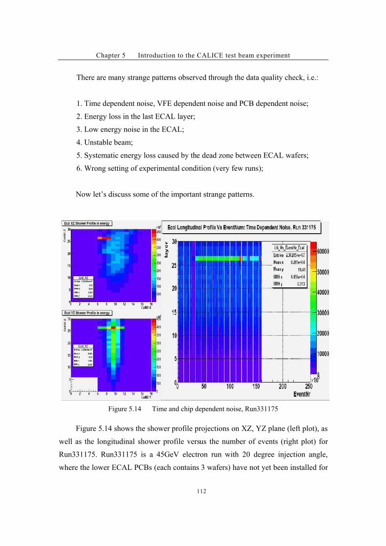
Chapter 5 Introduction to the CALICE test beam experiment
112
There are many strange patterns observed through the data quality check, i.e.:
1. Time dependent noise, VFE dependent noise and PCB dependent noise;
2. Energy loss in the last ECAL layer;
3. Low energy noise in the ECAL;
4. Unstable beam;
5. Systematic energy loss caused by the dead zone between ECAL wafers;
6. Wrong setting of experimental condition (very few runs);
Now let’s discuss some of the important strange patterns.
Figure 5.14 Time and chip dependent noise, Run331175
Figure 5.14 shows the shower profile projections on XZ, YZ plane (left plot), as
well as the longitudinal shower profile versus the number of events (right plot) for
Run331175. Run331175 is a 45GeV electron run with 20 degree injection angle,
where the lower ECAL PCBs (each contains 3 wafers) have not yet been installed for
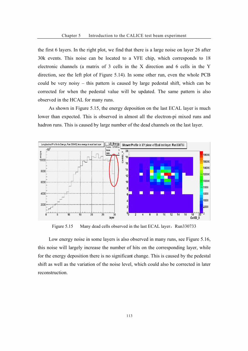
Chapter 5 Introduction to the CALICE test beam experiment
113
the first 6 layers. In the right plot, we find that there is a large noise on layer 26 after
30k events. This noise can be located to a VFE chip, which corresponds to 18
electronic channels (a matrix of 3 cells in the X direction and 6 cells in the Y
direction, see the left plot of Figure 5.14). In some other run, even the whole PCB
could be very noisy – this pattern is caused by large pedestal shift, which can be
corrected for when the pedestal value will be updated. The same pattern is also
observed in the HCAL for many runs.
As shown in Figure 5.15, the energy deposition on the last ECAL layer is much
lower than expected. This is observed in almost all the electron-pi mixed runs and
hadron runs. This is caused by large number of the dead channels on the last layer.
Figure 5.15 Many dead cells observed in the last ECAL layer"Run330733
Low energy noise in some layers is also observed in many runs, see Figure 5.16,
this noise will largely increase the number of hits on the corresponding layer, while
for the energy deposition there is no significant change. This is caused by the pedestal
shift as well as the variation of the noise level, which could also be corrected in later
reconstruction.
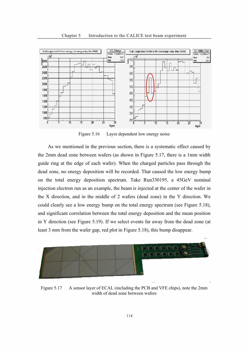
Chapter 5 Introduction to the CALICE test beam experiment
114
Figure 5.16 Layer dependent low energy noise
As we mentioned in the previous section, there is a systematic effect caused by
the 2mm dead zone between wafers (as shown in Figure 5.17, there is a 1mm width
guide ring at the edge of each wafer). When the charged particles pass through the
dead zone, no energy deposition will be recorded. That caused the low energy bump
on the total energy deposition spectrum. Take Run330195, a 45GeV nominal
injection electron run as an example, the beam is injected at the center of the wafer in
the X direction, and in the middle of 2 wafers (dead zone) in the Y direction. We
could clearly see a low energy bump on the total energy spectrum (see Figure 5.18),
and significant correlation between the total energy deposition and the mean position
in Y direction (see Figure 5.19). If we select events far away from the dead zone (at
least 3 mm from the wafer gap, red plot in Figure 5.18), this bump disappear.
Figure 5.17 A sensor layer of ECAL (including the PCB and VFE chips), note the 2mm
width of dead zone between wafers
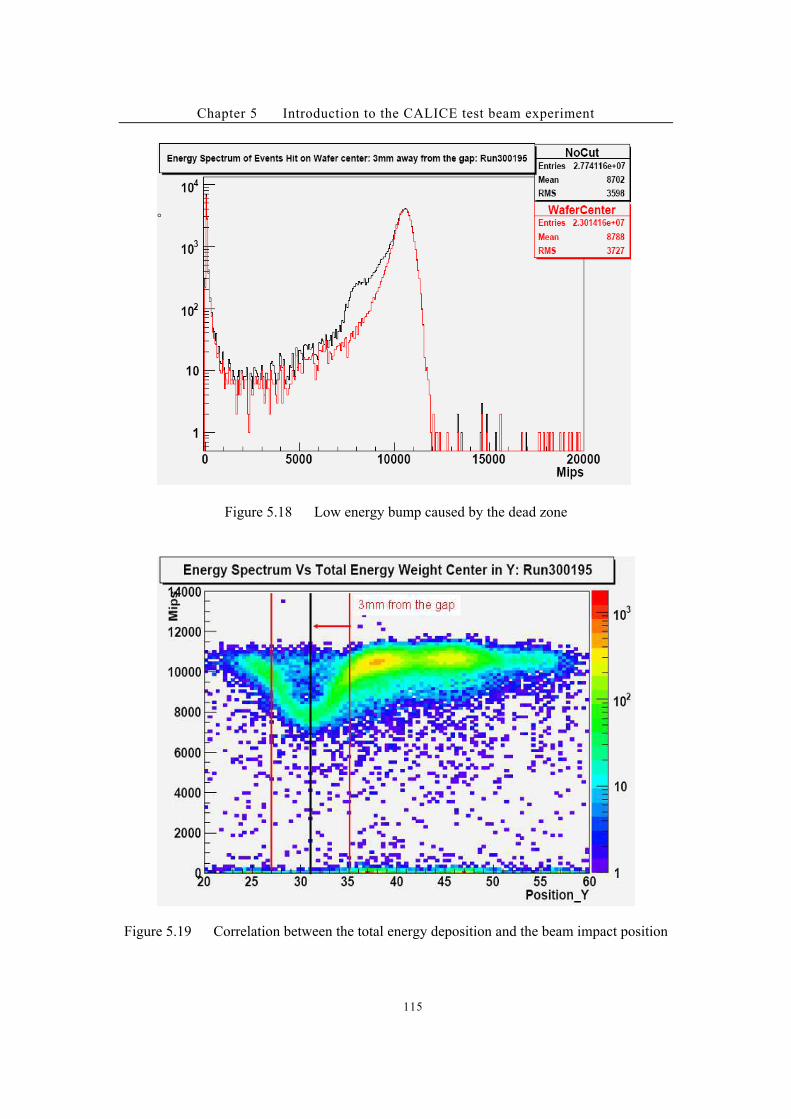
Chapter 5 Introduction to the CALICE test beam experiment
115
,
Figure 5.18 Low energy bump caused by the dead zone
Figure 5.19 Correlation between the total energy deposition and the beam impact position
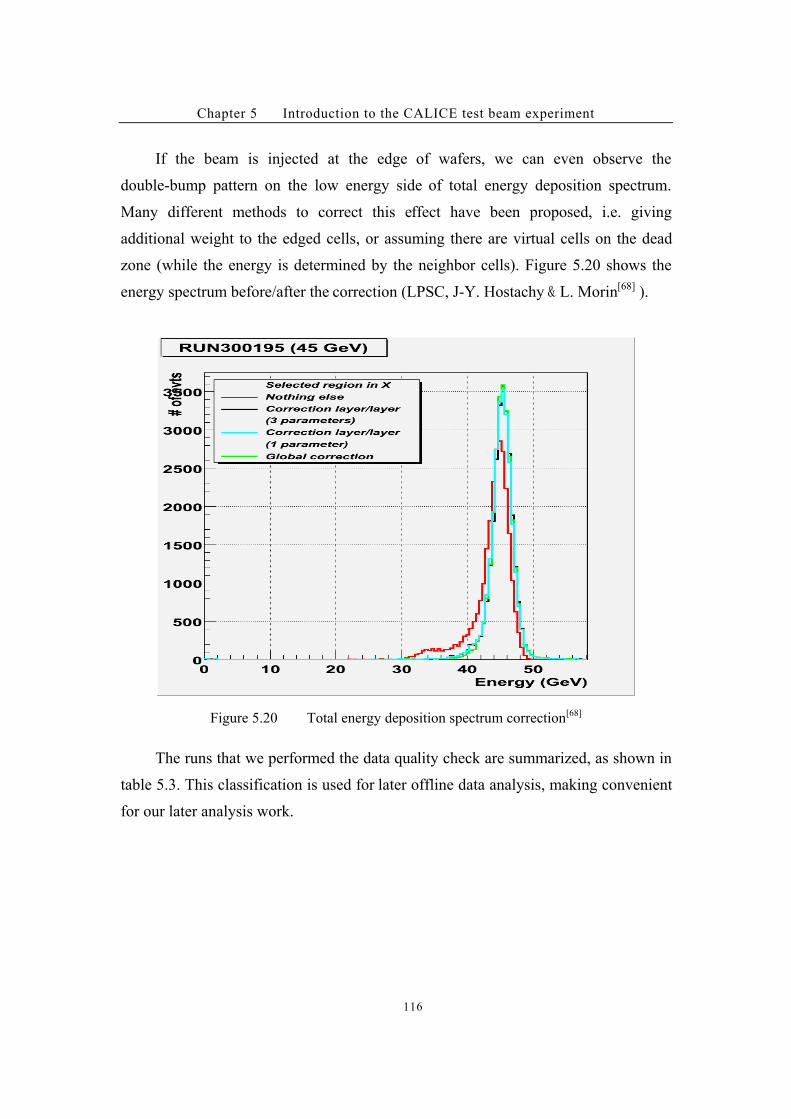
Chapter 5 Introduction to the CALICE test beam experiment
116
If the beam is injected at the edge of wafers, we can even observe the
double-bump pattern on the low energy side of total energy deposition spectrum.
Many different methods to correct this effect have been proposed, i.e. giving
additional weight to the edged cells, or assuming there are virtual cells on the dead
zone (while the energy is determined by the neighbor cells). Figure 5.20 shows the
energy spectrum before/after the correction (LPSC, J-Y. Hostachy - L. Morin[68]
).
. 5.21/01234
Figure 5.20 Total energy deposition spectrum correction[68]
The runs that we performed the data quality check are summarized, as shown in
table 5.3. This classification is used for later offline data analysis, making convenient
for our later analysis work.
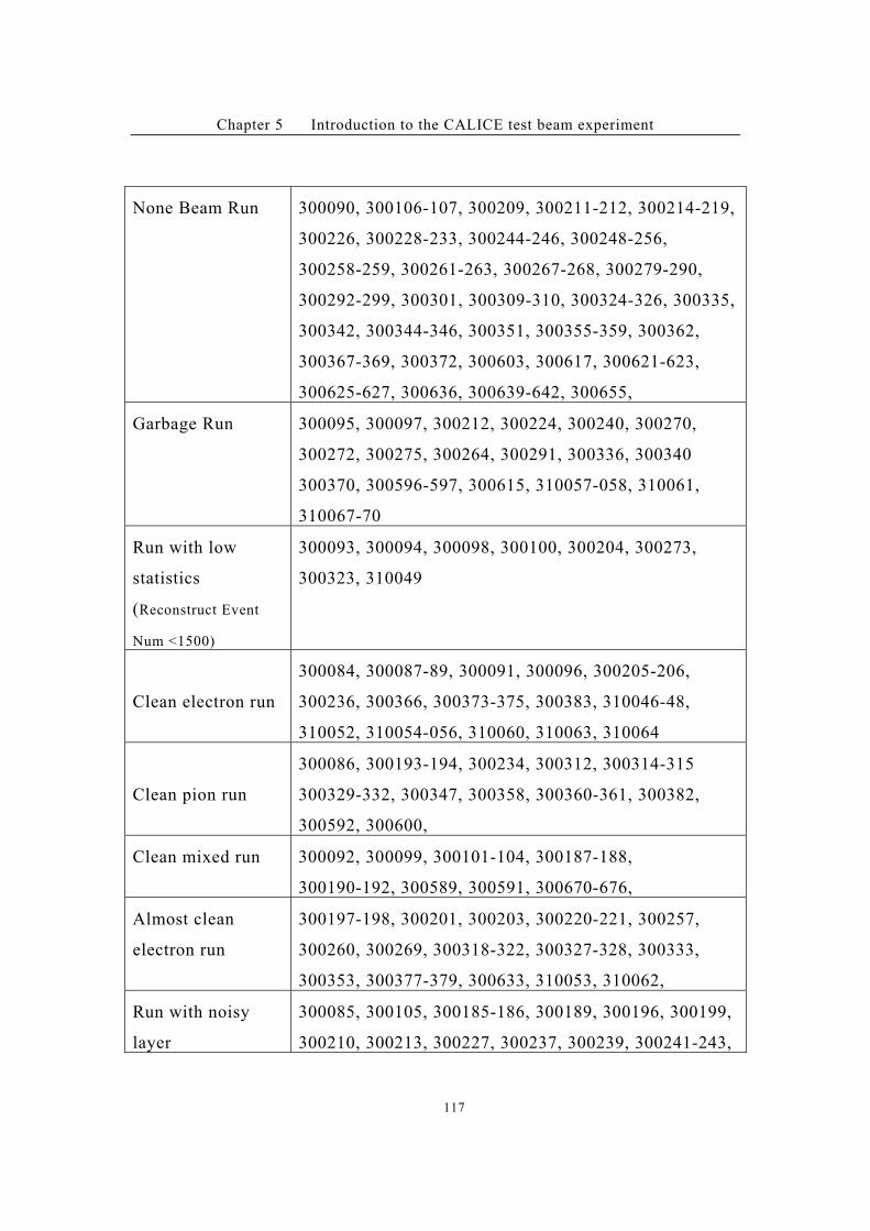
Chapter 5 Introduction to the CALICE test beam experiment
117
None Beam Run 300090, 300106-107, 300209, 300211-212, 300214-219,
300226, 300228-233, 300244-246, 300248-256,
300258-259, 300261-263, 300267-268, 300279-290,
300292-299, 300301, 300309-310, 300324-326, 300335,
300342, 300344-346, 300351, 300355-359, 300362,
300367-369, 300372, 300603, 300617, 300621-623,
300625-627, 300636, 300639-642, 300655,
Garbage Run 300095, 300097, 300212, 300224, 300240, 300270,
300272, 300275, 300264, 300291, 300336, 300340
300370, 300596-597, 300615, 310057-058, 310061,
310067-70
Run with low
statistics
(Reconstruct Event
Num <1500)
300093, 300094, 300098, 300100, 300204, 300273,
300323, 310049
Clean electron run
300084, 300087-89, 300091, 300096, 300205-206,
300236, 300366, 300373-375, 300383, 310046-48,
310052, 310054-056, 310060, 310063, 310064
Clean pion run
300086, 300193-194, 300234, 300312, 300314-315
300329-332, 300347, 300358, 300360-361, 300382,
300592, 300600,
Clean mixed run 300092, 300099, 300101-104, 300187-188,
300190-192, 300589, 300591, 300670-676,
Almost clean
electron run
300197-198, 300201, 300203, 300220-221, 300257,
300260, 300269, 300318-322, 300327-328, 300333,
300353, 300377-379, 300633, 310053, 310062,
Run with noisy
layer
300085, 300105, 300185-186, 300189, 300196, 300199,
300210, 300213, 300227, 300237, 300239, 300241-243,
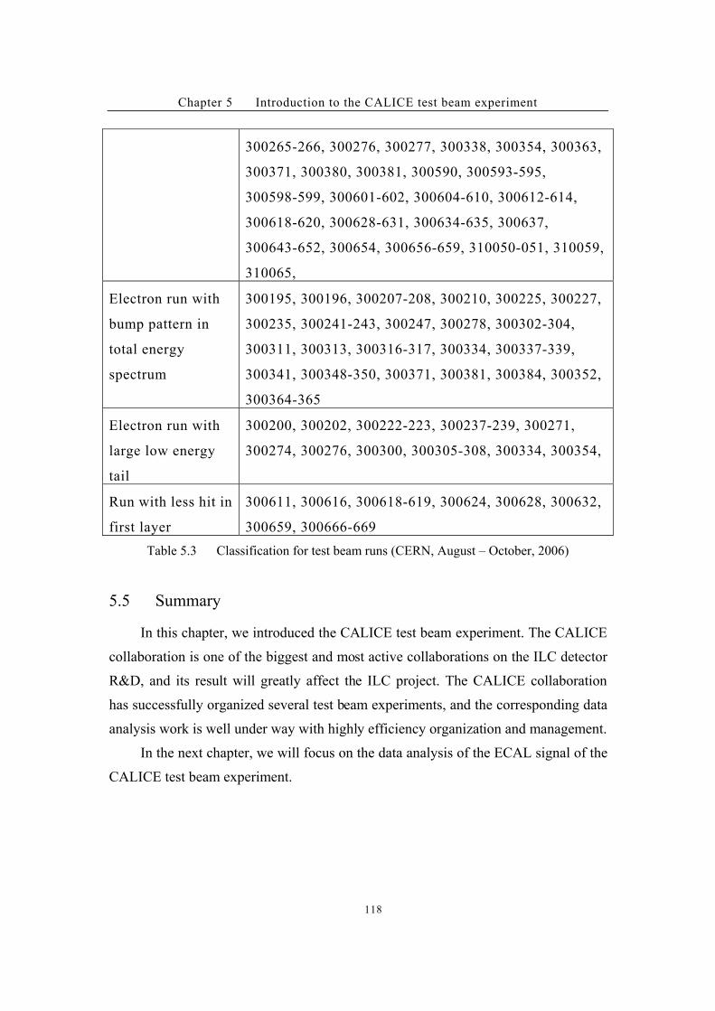
Chapter 5 Introduction to the CALICE test beam experiment
118
300265-266, 300276, 300277, 300338, 300354, 300363,
300371, 300380, 300381, 300590, 300593-595,
300598-599, 300601-602, 300604-610, 300612-614,
300618-620, 300628-631, 300634-635, 300637,
300643-652, 300654, 300656-659, 310050-051, 310059,
310065,
Electron run with
bump pattern in
total energy
spectrum
300195, 300196, 300207-208, 300210, 300225, 300227,
300235, 300241-243, 300247, 300278, 300302-304,
300311, 300313, 300316-317, 300334, 300337-339,
300341, 300348-350, 300371, 300381, 300384, 300352,
300364-365
Electron run with
large low energy
tail
300200, 300202, 300222-223, 300237-239, 300271,
300274, 300276, 300300, 300305-308, 300334, 300354,
Run with less hit in
first layer
300611, 300616, 300618-619, 300624, 300628, 300632,
300659, 300666-669
Table 5.3 Classification for test beam runs (CERN, August – October, 2006)
5.5 !Summary
In this chapter, we introduced the CALICE test beam experiment. The CALICE
collaboration is one of the biggest and most active collaborations on the ILC detector
R&D, and its result will greatly affect the ILC project. The CALICE collaboration
has successfully organized several test beam experiments, and the corresponding data
analysis work is well under way with highly efficiency organization and management.
In the next chapter, we will focus on the data analysis of the ECAL signal of the
CALICE test beam experiment.
Chapter 6 CALICE test beam data analysis, ECAL part
119
Chapter 6 CALICE test beam data analysis, ECAL
part
6.1 Introduction: interactions between particles and materials
Showers are created when beam particles inject into the calorimeter. The
electromagnetic shower create huge number of charged particles (mainly in
the absorber), and when those particles passing through the sensor layer, the
materials are ionized and create free charges. Driven by the electric field the
ionized electrons shift to the edge of sensor layer, and are collected by the
capacitance there. The quantity of the charge, which is proportional to the
number of charged particles passing through the sensor, is converted to the
voltages and then ADC values in the electronic. The energy deposition in each
calorimeter cell is assumed to be proportional to the quanta of charge, so by
pedestal subtraction, calibration and ADC value counting of each channel, we
are able to calculate how much energy is deposited in each cell.
For the calorimeter, an inject particle means a set of hits with their
positions and energy depositions information. The total energy deposition, the
beam inject position and inject angle could be calculated with those
information. In this chapter, we will discuss the energy, position and angle
resolution algorithm and accuracy for the ECAL in the CALICE test beam
experiment. To get a better understanding to the physical picture, we will first
discuss the interactions between different beam particles and the calorimeters.
The electron density is very high in materials, thus the electromagnetic
interaction of electron, positron and photon to the material is very strong. For
different materials, the conception of radiation length X0 is introduced to
describe the strength of their interaction with electron/positron/photon. The
energy flow density will be reduced by a factor of e when electron beam
passing through one X0 of material. X0 is approximately 7/9 of the electron
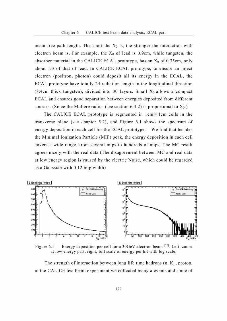
Chapter 6 CALICE test beam data analysis, ECAL part
120
mean free path length. The short the X0 is, the stronger the interaction with
electron beam is. For example, the X0 of lead is 0.9cm, while tungsten, the
absorber material in the CALICE ECAL prototype, has an X0 of 0.35cm, only
about 1/3 of that of lead. In CALICE ECAL prototype, to ensure an inject
electron (positron, photon) could deposit all its energy in the ECAL, the
ECAL prototype have totally 24 radiation length in the longitudinal direction
(8.4cm thick tungsten), divided into 30 layers. Small X0 allows a compact
ECAL and ensures good separation between energies deposited from different
sources. (Since the Moliere radius (see section 6.3.2) is proportional to X0.)
The CALICE ECAL prototype is segmented in 1cm#1cm cells in the
transverse plane (see chapter 5.2), and Figure 6.1 shows the spectrum of
energy deposition in each cell for the ECAL prototype. We find that besides
the Minimal Ionization Particle (MIP) peak, the energy deposition in each cell
covers a wide range, from several mips to hundreds of mips. The MC result
agrees nicely with the real data (The disagreement between MC and real data
at low energy region is caused by the electric Noise, which could be regarded
as a Gaussian with 0.12 mip width).
Figure 6.1 Energy deposition per cell for a 30GeV electron beam [57]. Left, zoom
at low energy part; right, full scale of energy per hit with log scale.
The strength of interaction between long life time hadrons (%, KL, proton,
in the CALICE test beam experiment we collected many % events and some of
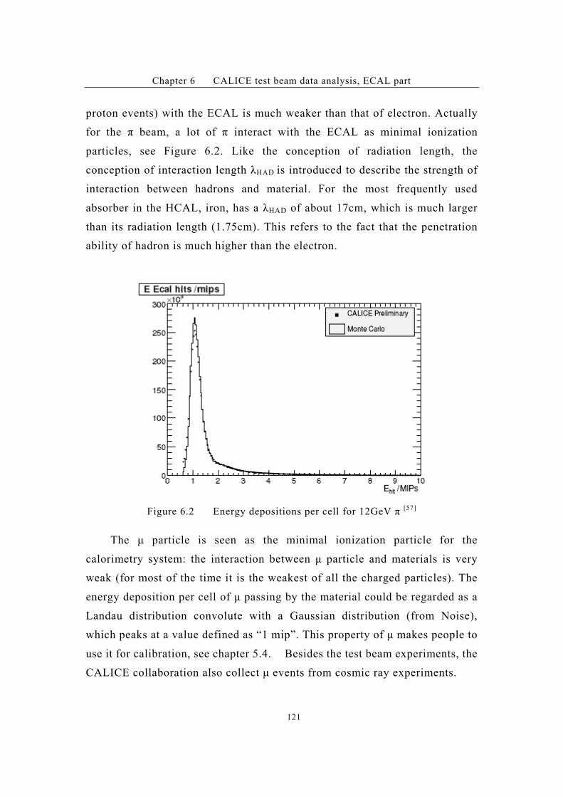
Chapter 6 CALICE test beam data analysis, ECAL part
121
proton events) with the ECAL is much weaker than that of electron. Actually
for the % beam, a lot of % interact with the ECAL as minimal ionization
particles, see Figure 6.2. Like the conception of radiation length, the
conception of interaction length 0HAD is introduced to describe the strength of
interaction between hadrons and material. For the most frequently used
absorber in the HCAL, iron, has a 0HAD of about 17cm, which is much larger
than its radiation length (1.75cm). This refers to the fact that the penetration
ability of hadron is much higher than the electron.
Figure 6.2 Energy depositions per cell for 12GeV % [57]
The # particle is seen as the minimal ionization particle for the
calorimetry system: the interaction between # particle and materials is very
weak (for most of the time it is the weakest of all the charged particles). The
energy deposition per cell of # passing by the material could be regarded as a
Landau distribution convolute with a Gaussian distribution (from Noise),
which peaks at a value defined as “1 mip”. This property of # makes people to
use it for calibration, see chapter 5.4. Besides the test beam experiments, the
CALICE collaboration also collect # events from cosmic ray experiments.
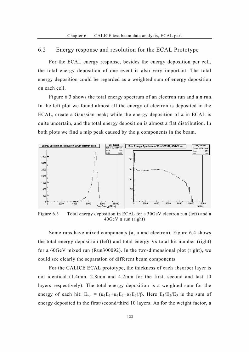
Chapter 6 CALICE test beam data analysis, ECAL part
122
6.2 Energy response and resolution for the ECAL Prototype
For the ECAL energy response, besides the energy deposition per cell,
the total energy deposition of one event is also very important. The total
energy deposition could be regarded as a weighted sum of energy deposition
on each cell.
Figure 6.3 shows the total energy spectrum of an electron run and a % run.
In the left plot we found almost all the energy of electron is deposited in the
ECAL, create a Gaussian peak; while the energy deposition of % in ECAL is
quite uncertain, and the total energy deposition is almost a flat distribution. In
both plots we find a mip peak caused by the # components in the beam.
Figure 6.3 Total energy deposition in ECAL for a 30GeV electron run (left) and a
40GeV % run (right)
Some runs have mixed components (%, # and electron). Figure 6.4 shows
the total energy deposition (left) and total energy Vs total hit number (right)
for a 60GeV mixed run (Run300092). In the two-dimensional plot (right), we
could see clearly the separation of different beam components.
For the CALICE ECAL prototype, the thickness of each absorber layer is
not identical (1.4mm, 2.8mm and 4.2mm for the first, second and last 10
layers respectively). The total energy deposition is a weighted sum for the
energy of each hit: Etot = (11E1+12E2+13E3)//. Here E1/E2/E3 is the sum of
energy deposited in the first/second/third 10 layers. As for the weight factor, a
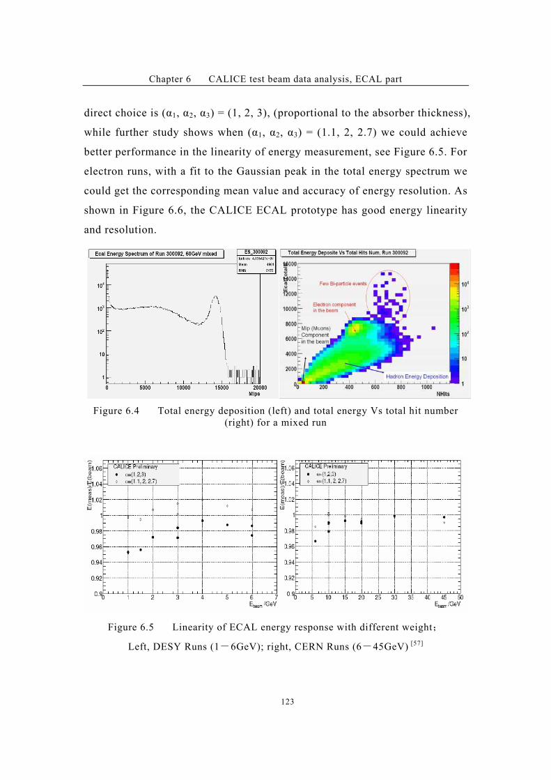
Chapter 6 CALICE test beam data analysis, ECAL part
123
direct choice is (11, 12, 13) = (1, 2, 3), (proportional to the absorber thickness),
while further study shows when (11, 12, 13) = (1.1, 2, 2.7) we could achieve
better performance in the linearity of energy measurement, see Figure 6.5. For
electron runs, with a fit to the Gaussian peak in the total energy spectrum we
could get the corresponding mean value and accuracy of energy resolution. As
shown in Figure 6.6, the CALICE ECAL prototype has good energy linearity
and resolution.
Figure 6.4 Total energy deposition (left) and total energy Vs total hit number
(right) for a mixed run
Figure 6.5 Linearity of ECAL energy response with different weight%
Left, DESY Runs (1*6GeV); right, CERN Runs (6*45GeV) [57]
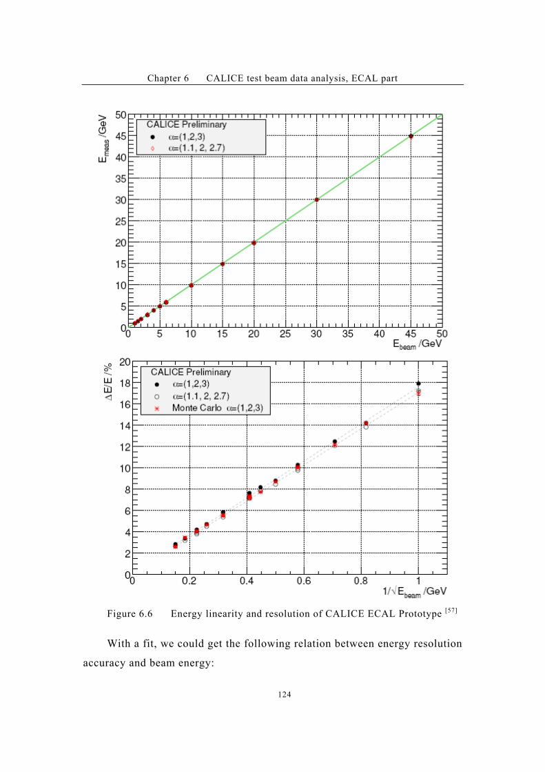
Chapter 6 CALICE test beam data analysis, ECAL part
124
Figure 6.6 Energy linearity and resolution of CALICE ECAL Prototype [57]
With a fit, we could get the following relation between energy resolution
accuracy and beam energy:
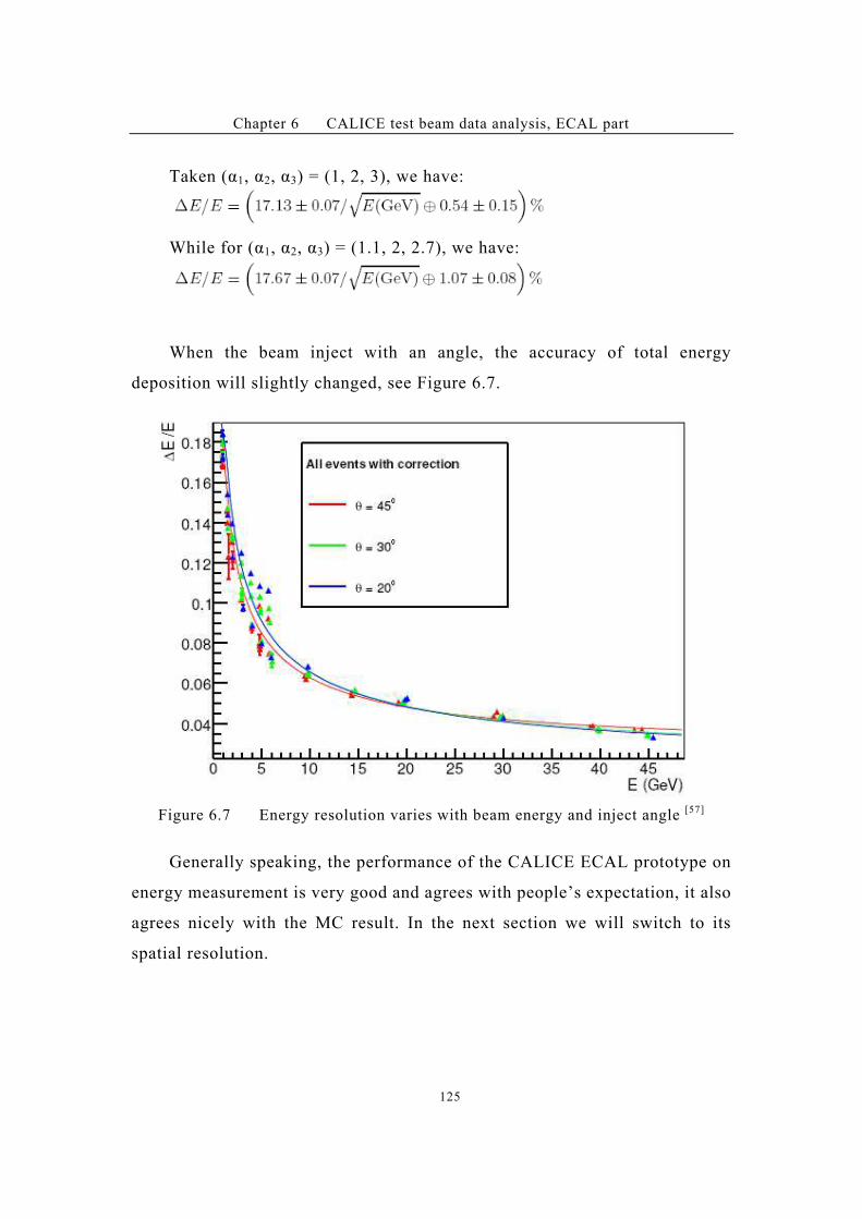
Chapter 6 CALICE test beam data analysis, ECAL part
125
Taken (11, 12, 13) = (1, 2, 3), we have:
While for (11, 12, 13) = (1.1, 2, 2.7), we have:
When the beam inject with an angle, the accuracy of total energy
deposition will slightly changed, see Figure 6.7.
Figure 6.7 Energy resolution varies with beam energy and inject angle [57]
Generally speaking, the performance of the CALICE ECAL prototype on
energy measurement is very good and agrees with people’s expectation, it also
agrees nicely with the MC result. In the next section we will switch to its
spatial resolution.
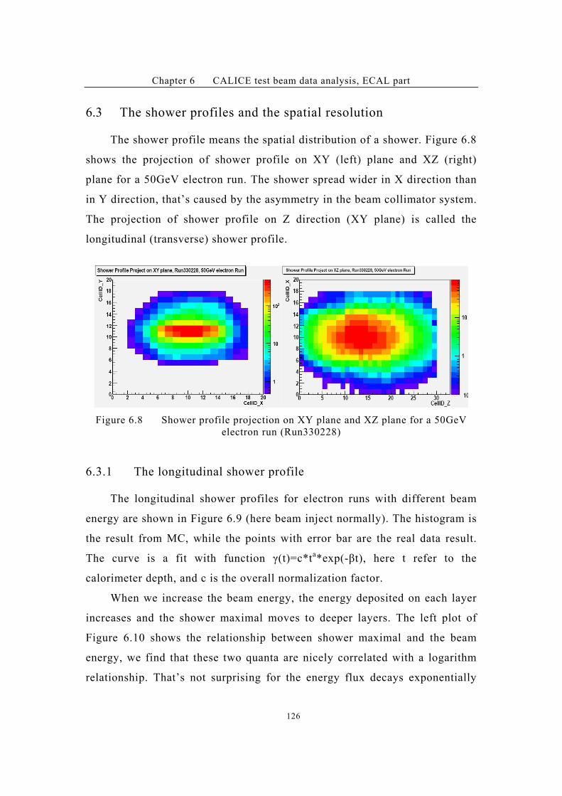
Chapter 6 CALICE test beam data analysis, ECAL part
126
6.3 The shower profiles and the spatial resolution
The shower profile means the spatial distribution of a shower. Figure 6.8
shows the projection of shower profile on XY (left) plane and XZ (right)
plane for a 50GeV electron run. The shower spread wider in X direction than
in Y direction, that’s caused by the asymmetry in the beam collimator system.
The projection of shower profile on Z direction (XY plane) is called the
longitudinal (transverse) shower profile.
Figure 6.8 Shower profile projection on XY plane and XZ plane for a 50GeV
electron run (Run330228)
6.3.1 The longitudinal shower profile
The longitudinal shower profiles for electron runs with different beam
energy are shown in Figure 6.9 (here beam inject normally). The histogram is
the result from MC, while the points with error bar are the real data result.
The curve is a fit with function )(t)=c*ta*exp(-/t), here t refer to the
calorimeter depth, and c is the overall normalization factor.
When we increase the beam energy, the energy deposited on each layer
increases and the shower maximal moves to deeper layers. The left plot of
Figure 6.10 shows the relationship between shower maximal and the beam
energy, we find that these two quanta are nicely correlated with a logarithm
relationship. That’s not surprising for the energy flux decays exponentially
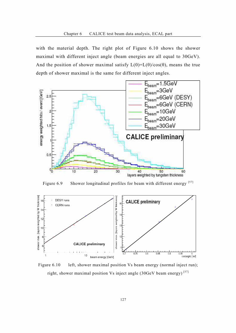
Chapter 6 CALICE test beam data analysis, ECAL part
127
with the material depth. The right plot of Figure 6.10 shows the shower
maximal with different inject angle (beam energies are all equal to 30GeV).
And the position of shower maximal satisfy L(0)=L(')/cos('), means the true
depth of shower maximal is the same for different inject angles.
Figure 6.9 Shower longitudinal profiles for beam with different energy [57]
Figure 6.10 left, shower maximal position Vs beam energy (normal inject run);
right, shower maximal position Vs inject angle (30GeV beam energy) [57]
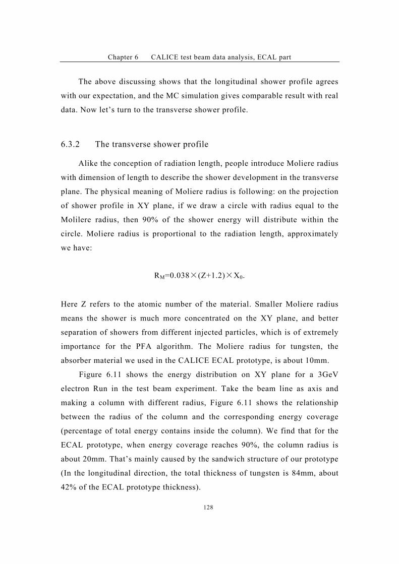
Chapter 6 CALICE test beam data analysis, ECAL part
128
The above discussing shows that the longitudinal shower profile agrees
with our expectation, and the MC simulation gives comparable result with real
data. Now let’s turn to the transverse shower profile.
6.3.2 The transverse shower profile
Alike the conception of radiation length, people introduce Moliere radius
with dimension of length to describe the shower development in the transverse
plane. The physical meaning of Moliere radius is following: on the projection
of shower profile in XY plane, if we draw a circle with radius equal to the
Molilere radius, then 90% of the shower energy will distribute within the
circle. Moliere radius is proportional to the radiation length, approximately
we have:
RM=0.038#(Z+1.2)#X0.
Here Z refers to the atomic number of the material. Smaller Moliere radius
means the shower is much more concentrated on the XY plane, and better
separation of showers from different injected particles, which is of extremely
importance for the PFA algorithm. The Moliere radius for tungsten, the
absorber material we used in the CALICE ECAL prototype, is about 10mm.
Figure 6.11 shows the energy distribution on XY plane for a 3GeV
electron Run in the test beam experiment. Take the beam line as axis and
making a column with different radius, Figure 6.11 shows the relationship
between the radius of the column and the corresponding energy coverage
(percentage of total energy contains inside the column). We find that for the
ECAL prototype, when energy coverage reaches 90%, the column radius is
about 20mm. That’s mainly caused by the sandwich structure of our prototype
(In the longitudinal direction, the total thickness of tungsten is 84mm, about
42% of the ECAL prototype thickness).
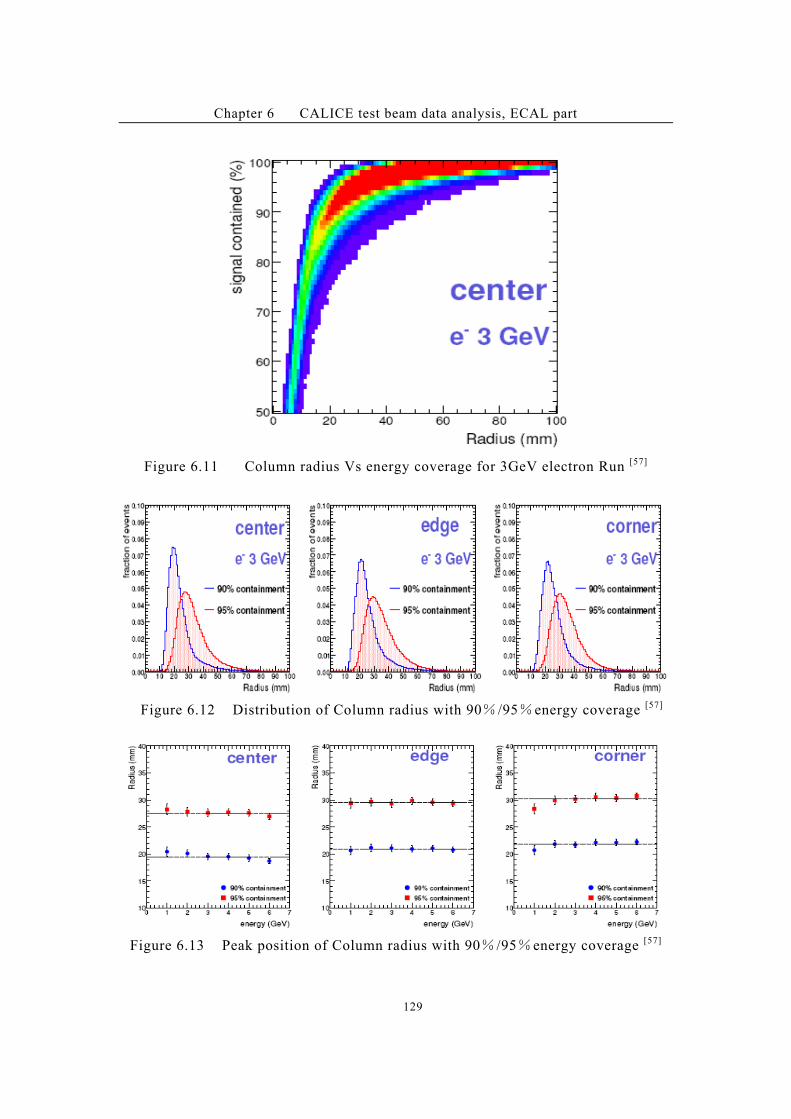
Chapter 6 CALICE test beam data analysis, ECAL part
129
Figure 6.11 Column radius Vs energy coverage for 3GeV electron Run [57]
Figure 6.12 Distribution of Column radius with 90+ /95+energy coverage [57]
Figure 6.13 Peak position of Column radius with 90+ /95+energy coverage [57]
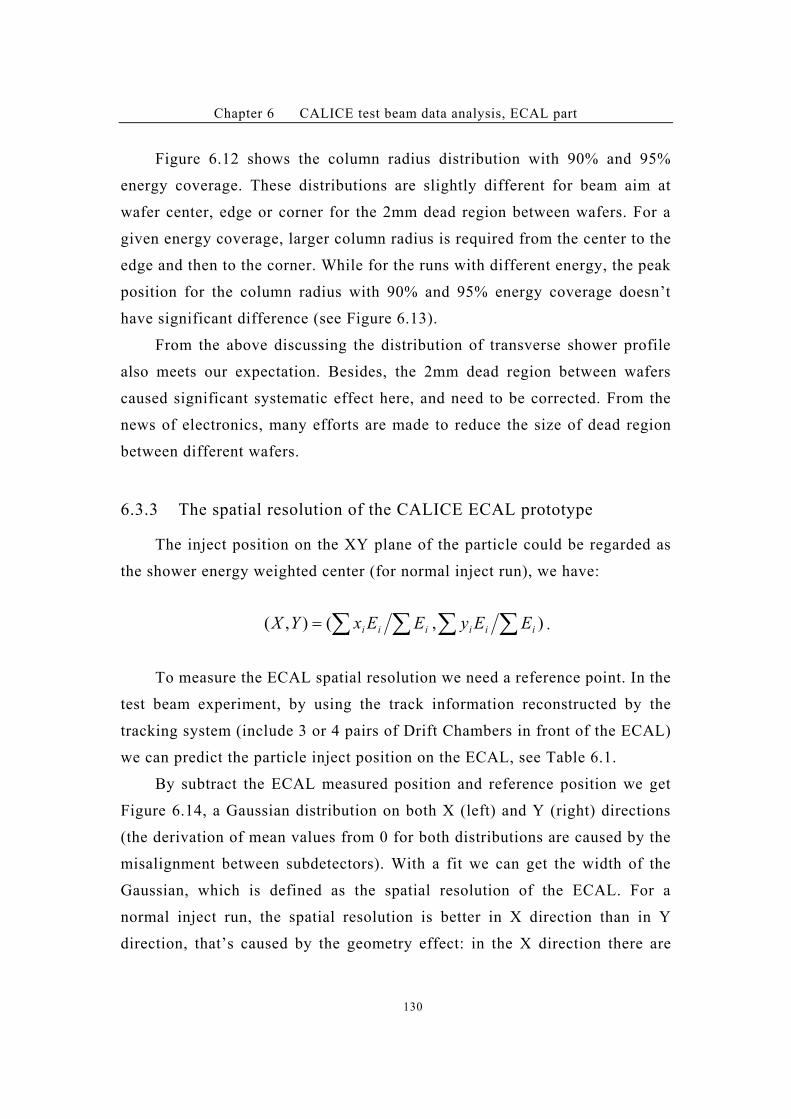
Chapter 6 CALICE test beam data analysis, ECAL part
130
Figure 6.12 shows the column radius distribution with 90% and 95%
energy coverage. These distributions are slightly different for beam aim at
wafer center, edge or corner for the 2mm dead region between wafers. For a
given energy coverage, larger column radius is required from the center to the
edge and then to the corner. While for the runs with different energy, the peak
position for the column radius with 90% and 95% energy coverage doesn’t
have significant difference (see Figure 6.13).
From the above discussing the distribution of transverse shower profile
also meets our expectation. Besides, the 2mm dead region between wafers
caused significant systematic effect here, and need to be corrected. From the
news of electronics, many efforts are made to reduce the size of dead region
between different wafers.
6.3.3 The spatial resolution of the CALICE ECAL prototype
The inject position on the XY plane of the particle could be regarded as
the shower energy weighted center (for normal inject run), we have:
),(),( ;;;;' iiiiii EEyEExYX .
To measure the ECAL spatial resolution we need a reference point. In the
test beam experiment, by using the track information reconstructed by the
tracking system (include 3 or 4 pairs of Drift Chambers in front of the ECAL)
we can predict the particle inject position on the ECAL, see Table 6.1.
By subtract the ECAL measured position and reference position we get
Figure 6.14, a Gaussian distribution on both X (left) and Y (right) directions
(the derivation of mean values from 0 for both distributions are caused by the
misalignment between subdetectors). With a fit we can get the width of the
Gaussian, which is defined as the spatial resolution of the ECAL. For a
normal inject run, the spatial resolution is better in X direction than in Y
direction, that’s caused by the geometry effect: in the X direction there are
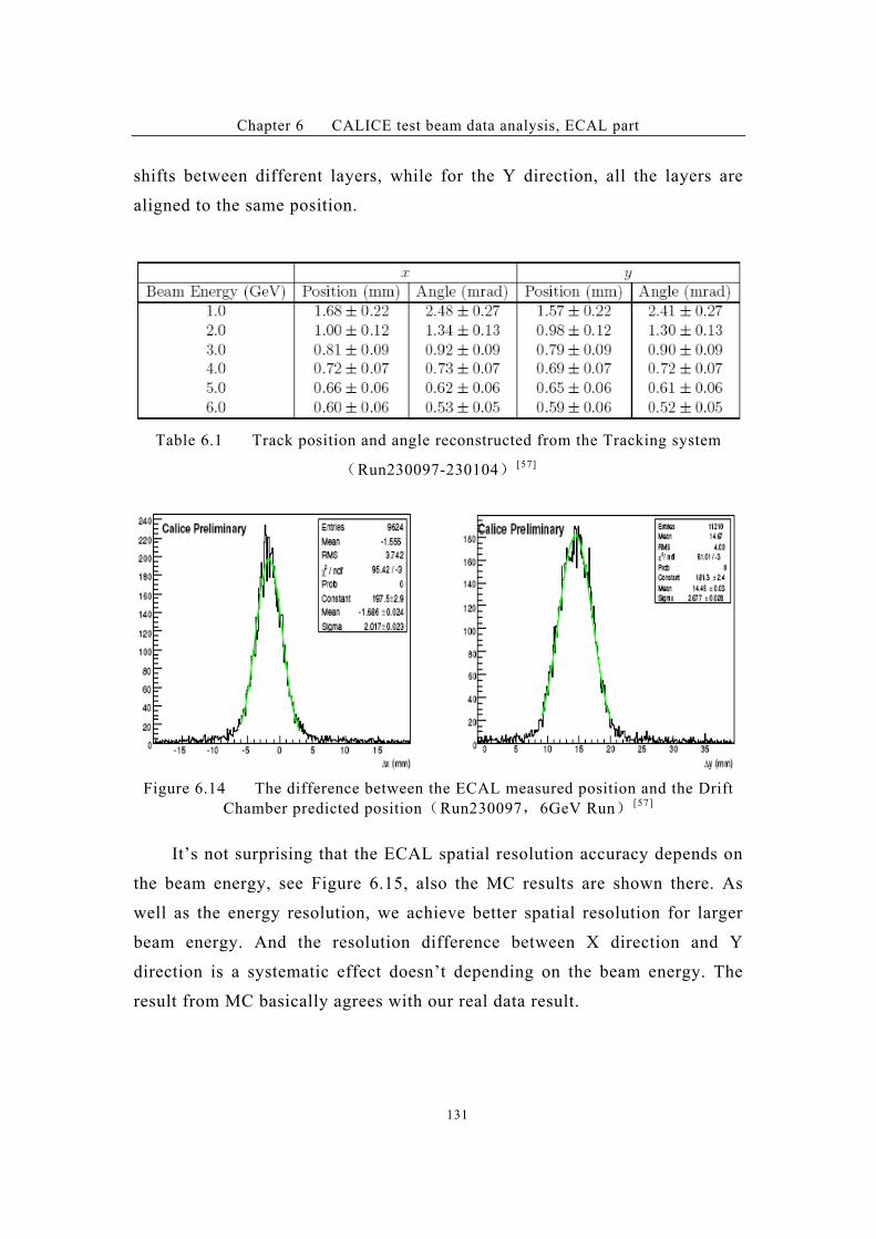
Chapter 6 CALICE test beam data analysis, ECAL part
131
shifts between different layers, while for the Y direction, all the layers are
aligned to the same position.
Table 6.1 Track position and angle reconstructed from the Tracking system
&Run230097-230104' [57]
Figure 6.14 The difference between the ECAL measured position and the Drift
Chamber predicted position&Run230097"6GeV Run' [57]
It’s not surprising that the ECAL spatial resolution accuracy depends on
the beam energy, see Figure 6.15, also the MC results are shown there. As
well as the energy resolution, we achieve better spatial resolution for larger
beam energy. And the resolution difference between X direction and Y
direction is a systematic effect doesn’t depending on the beam energy. The
result from MC basically agrees with our real data result.
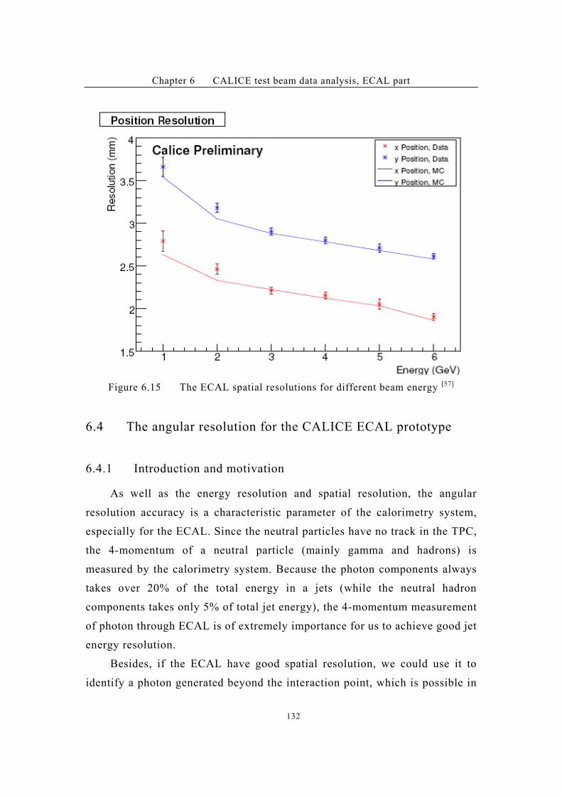
Chapter 6 CALICE test beam data analysis, ECAL part
132
Figure 6.15 The ECAL spatial resolutions for different beam energy [57]
6.4 The angular resolution for the CALICE ECAL prototype
6.4.1 Introduction and motivation
As well as the energy resolution and spatial resolution, the angular
resolution accuracy is a characteristic parameter of the calorimetry system,
especially for the ECAL. Since the neutral particles have no track in the TPC,
the 4-momentum of a neutral particle (mainly gamma and hadrons) is
measured by the calorimetry system. Because the photon components always
takes over 20% of the total energy in a jets (while the neutral hadron
components takes only 5% of total jet energy), the 4-momentum measurement
of photon through ECAL is of extremely importance for us to achieve good jet
energy resolution.
Besides, if the ECAL have good spatial resolution, we could use it to
identify a photon generated beyond the interaction point, which is possible in
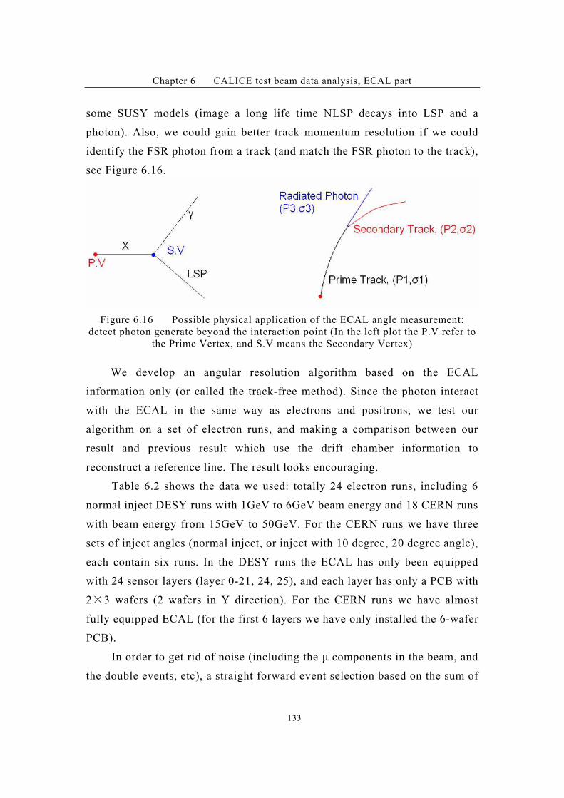
Chapter 6 CALICE test beam data analysis, ECAL part
133
some SUSY models (image a long life time NLSP decays into LSP and a
photon). Also, we could gain better track momentum resolution if we could
identify the FSR photon from a track (and match the FSR photon to the track),
see Figure 6.16.
Figure 6.16 Possible physical application of the ECAL angle measurement:
detect photon generate beyond the interaction point (In the left plot the P.V refer to
the Prime Vertex, and S.V means the Secondary Vertex)
We develop an angular resolution algorithm based on the ECAL
information only (or called the track-free method). Since the photon interact
with the ECAL in the same way as electrons and positrons, we test our
algorithm on a set of electron runs, and making a comparison between our
result and previous result which use the drift chamber information to
reconstruct a reference line. The result looks encouraging.
Table 6.2 shows the data we used: totally 24 electron runs, including 6
normal inject DESY runs with 1GeV to 6GeV beam energy and 18 CERN runs
with beam energy from 15GeV to 50GeV. For the CERN runs we have three
sets of inject angles (normal inject, or inject with 10 degree, 20 degree angle),
each contain six runs. In the DESY runs the ECAL has only been equipped
with 24 sensor layers (layer 0-21, 24, 25), and each layer has only a PCB with
2#3 wafers (2 wafers in Y direction). For the CERN runs we have almost
fully equipped ECAL (for the first 6 layers we have only installed the 6-wafer
PCB).
In order to get rid of noise (including the # components in the beam, and
the double events, etc), a straight forward event selection based on the sum of
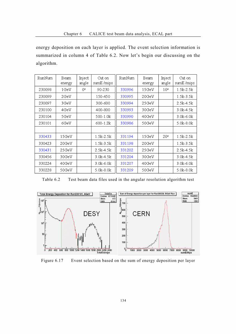
Chapter 6 CALICE test beam data analysis, ECAL part
134
energy deposition on each layer is applied. The event selection information is
summarized in column 4 of Table 6.2. Now let’s begin our discussing on the
algorithm.
Table 6.2 Test beam data files used in the angular resolution algorithm test
Figure 6.17 Event selection based on the sum of energy deposition per layer

Chapter 6 CALICE test beam data analysis, ECAL part
135
6.4.2 Angular resolution algorithm for the CALICE ECAL Prototype
We assume that in the absence of external magnetic field, the
longitudinal shower development of an electron/photon in the ECAL
continues in the direction of the beam. This direction should coincide with the
shower axis and the latter can be determined from a straight line fit to the
shower. The X and Y directions are treated separately assuming there is no
correlation between them. Here is the algorithm (take the X direction for
example):
First, hit selection for each event: a hit is taken into account when it has
energy deposition larger than 0.6mip.
Second, get a reference line with -2 fit to the energy weighted center per
layer, ( ),(),( ;;;;'j ijj ijijj ijj ijijii EEyEExYX , here index i denotes
the layer number and index j marks the hit number of the corresponding layer).
The -2 is defined as following:
Total energy deposited in each layer is used as an additional weight in
the -2. With the reference line, we are able to calculate the distance between
the intersection point (of the reference line and the layer plane) and energy
weighted center for each layer. The distribution of this distance is always a
Gaussian, while its width could be defined as the spatial resolution of this
layer, marked with *i, see Figure 6.18.
Third, taken into account the spatial resolution per layer, and fit the
energy weighted centers into a straight line again. We have:
The direction of the fitted line is defined as the direction of inject beam. Thus
the beam angle is measured.
= >;'
##'
30
12
2
2
i
i
i
ii Ebazx
)?
= >;'
##'n
i
iii EbaZX1
22?
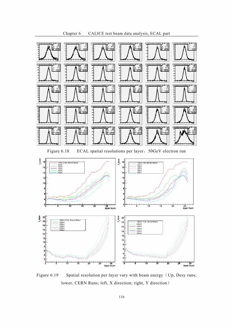
Chapter 6 CALICE test beam data analysis, ECAL part
136
Figure 6.18 ECAL spatial resolutions per layer"50GeV electron run
Figure 6.19 Spatial resolution per layer vary with beam energy&Up, Desy runs;
lower, CERN Runs; left, X direction; right, Y direction'
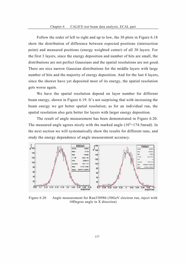
Chapter 6 CALICE test beam data analysis, ECAL part
137
Follow the order of left to right and up to low, the 30 plots in Figure 6.18
show the distribution of difference between expected positions (intersection
point) and measured positions (energy weighted center) of all 30 layers. For
the first 3 layers, since the energy deposition and number of hits are small, the
distributions are not perfect Gaussians and the spatial resolutions are not good.
There are nice narrow Gaussian distributions for the middle layers with large
number of hits and the majority of energy deposition. And for the last 4 layers,
since the shower have yet deposited most of its energy, the spatial resolution
gets worse again.
We have the spatial resolution depend on layer number for different
beam energy, shown in Figure 6.19. It’s not surprising that with increasing the
beam energy we get better spatial resolution; as for an individual run, the
spatial resolution also gets better for layers with larger energy deposition.
The result of angle measurement has been demonstrated in Figure 6.20.
The measured angle agrees nicely with the marked angle (10o=174.5mrad). In
the next section we will systematically show the results for different runs, and
study the energy dependence of angle measurement accuracy.
Figure 6.20 Angle measurement for Run330986 (50GeV electron run, inject with
10Degree angle in X direction)
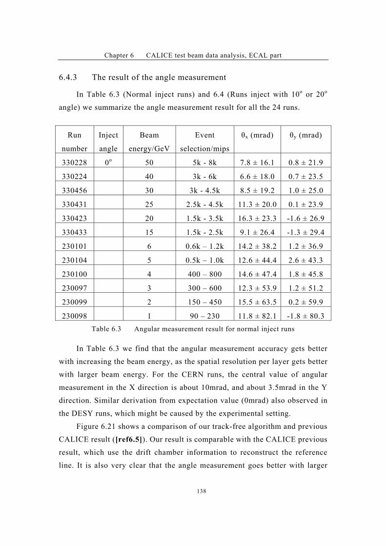
Chapter 6 CALICE test beam data analysis, ECAL part
138
6.4.3 The result of the angle measurement
In Table 6.3 (Normal inject runs) and 6.4 (Runs inject with 10o or 20
o
angle) we summarize the angle measurement result for all the 24 runs.
Run
number
Inject
angle
Beam
energy/GeV
Event
selection/mips
'x (mrad) 'y (mrad)
330228 0o 50 5k - 8k 7.8 ± 16.1 0.8 ± 21.9
330224 40 3k - 6k 6.6 ± 18.0 0.7 ± 23.5
330456 30 3k - 4.5k 8.5 ± 19.2 1.0 ± 25.0
330431 25 2.5k - 4.5k 11.3 ± 20.0 0.1 ± 23.9
330423 20 1.5k - 3.5k 16.3 ± 23.3 -1.6 ± 26.9
330433 15 1.5k - 2.5k 9.1 ± 26.4 -1.3 ± 29.4
230101 6 0.6k – 1.2k 14.2 ± 38.2 1.2 ± 36.9
230104 5 0.5k – 1.0k 12.6 ± 44.4 2.6 ± 43.3
230100 4 400 – 800 14.6 ± 47.4 1.8 ± 45.8
230097 3 300 – 600 12.3 ± 53.9 1.2 ± 51.2
230099 2 150 – 450 15.5 ± 63.5 0.2 ± 59.9
230098 1 90 – 230 11.8 ± 82.1 -1.8 ± 80.3
Table 6.3 Angular measurement result for normal inject runs
In Table 6.3 we find that the angular measurement accuracy gets better
with increasing the beam energy, as the spatial resolution per layer gets better
with larger beam energy. For the CERN runs, the central value of angular
measurement in the X direction is about 10mrad, and about 3.5mrad in the Y
direction. Similar derivation from expectation value (0mrad) also observed in
the DESY runs, which might be caused by the experimental setting.
Figure 6.21 shows a comparison of our track-free algorithm and previous
CALICE result ([ref6.5]). Our result is comparable with the CALICE previous
result, which use the drift chamber information to reconstruct the reference
line. It is also very clear that the angle measurement goes better with larger
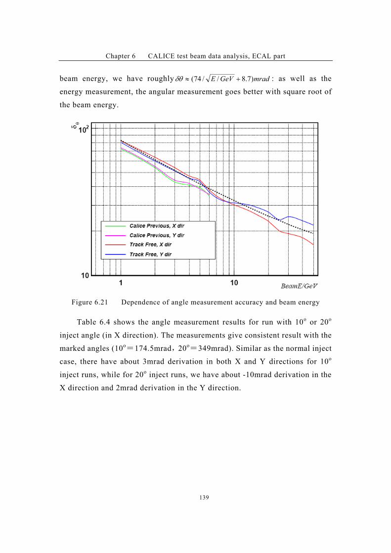
Chapter 6 CALICE test beam data analysis, ECAL part
139
beam energy, we have roughly mradGeVE )7.8//74( $01+ : as well as the
energy measurement, the angular measurement goes better with square root of
the beam energy.
Figure 6.21 Dependence of angle measurement accuracy and beam energy
Table 6.4 shows the angle measurement results for run with 10o or 20
o
inject angle (in X direction). The measurements give consistent result with the
marked angles (10o)174.5mrad"20
o)349mrad). Similar as the normal inject
case, there have about 3mrad derivation in both X and Y directions for 10o
inject runs, while for 20o inject runs, we have about -10mrad derivation in the
X direction and 2mrad derivation in the Y direction.
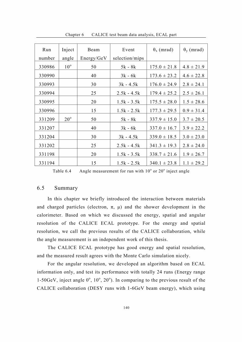
Chapter 6 CALICE test beam data analysis, ECAL part
140
Run
number
Inject
angle
Beam
Energy/GeV
Event
selection/mips
'x (mrad) 'y (mrad)
330986 10o 50 5k - 8k 175.0 ± 21.8 4.8 ± 21.9
330990 40 3k - 6k 173.6 ± 23.2 4.6 ± 22.8
330993 30 3k - 4.5k 176.0 ± 24.9 2.8 ± 24.1
330994 25 2.5k - 4.5k 179.4 ± 25.2 2.5 ± 26.1
330995 20 1.5k - 3.5k 175.5 ± 28.0 1.5 ± 28.6
330996 15 1.5k - 2.5k 177.3 ± 29.5 0.9 ± 31.4
331209 20o 50 5k - 8k 337.9 ± 15.0 3.7 ± 20.5
331207 40 3k - 6k 337.0 ± 16.7 3.9 ± 22.2
331204 30 3k - 4.5k 339.0 ± 18.5 3.0 ± 23.0
331202 25 2.5k - 4.5k 341.3 ± 19.3 2.8 ± 24.0
331198 20 1.5k - 3.5k 338.7 ± 21.6 1.9 ± 26.7
331194 15 1.5k - 2.5k 340.1 ± 23.8 1.1 ± 29.2
Table 6.4 Angle measurement for run with 10o or 20o inject angle
6.5 Summary
In this chapter we briefly introduced the interaction between materials
and charged particles (electron, %, #) and the shower development in the
calorimeter. Based on which we discussed the energy, spatial and angular
resolution of the CALICE ECAL prototype. For the energy and spatial
resolution, we call the previous results of the CALICE collaboration, while
the angle measurement is an independent work of this thesis.
The CALICE ECAL prototype has good energy and spatial resolution,
and the measured result agrees with the Monte Carlo simulation nicely.
For the angular resolution, we developed an algorithm based on ECAL
information only, and test its performance with totally 24 runs (Energy range
1-50GeV, inject angle 0o, 10
o, 20
o). In comparing to the previous result of the
CALICE collaboration (DESY runs with 1-6GeV beam energy), which using

Chapter 6 CALICE test beam data analysis, ECAL part
141
the drift chamber resolved track as reference, we find our result is comparable
with previous result for 1-3GeV beam energy, while our result is slightly
better than the previous result for 4-6GeV beam energy.
With our algorithm, the measured angle agrees with the expected angle,
We found that the angular resolution is fit well by a function varying with the square
root of the beam energy (as the energy resolution), and we were able to achieve a
precision of approximately mradGeVE )7.8//74( $01+ in the angular resolution.
Chapter 7 Summary and perspective
142
Chapter 7 Summary and perspective
7.1 Summary of the thesis
This thesis has mainly focused on ILC detector studies. Contributions of this
thesis are mainly twofold: first, the analysis of Higgs boson mass and cross section
measurements at the ILC (with full simulation of the !!HHZee ""#$channel
and corresponding backgrounds); second, an analysis of CALICE test beam data. A
preliminary study on beam parameter selection has also been performed.
The detector is a very complex system, and its exact performance is difficult to
predict solely via theoretical calculations. Before its construction, numerous Monte
Carlo simulations and test beam experiments must be performed to ensure that the
detector can achieve its optimal performance. The sequence of detector R&D then
goes something like the following:
First, develop Monte Carlo tools and perform test beam experiments where feasible.
As noted in pervious chapters, the ILC detector is required to achieve a jet
energy resolution of GeVE //3.0 , which is roughly twice as good as that
achieved during the LEP experiments. This precision may be achieved
via a PFA algorithm and an extremely high degree of spatial granularity
in the calorimetry system. Members of the CALICE collaboration have
constructed a prototype calorimeter including ECAL, HCAL and TCMT
elements. This prototype has been studied in test beam experiments, and
one of the important works of this thesis is to analyze data from said
experiments.
Second, virtualize the detector utilizing Monte Carlo tools and test its performance
for different physical processes with different detector geometries and settings.
Though this step, one or more reliable detector concepts may be developed.
Chapter 7 Summary and perspective
143
This process is known as detector optimization study, and it requires huge
amounts of computational resources – since full simulations on a set of
benchmark channels must be performed under various detector concepts. The
application of grid tools is mandatory for this study. The organization and
management of the detector optimization project is very important (That’s why
people formed the ILD collaboration). For this detector optimization study, we
have studied Higgs mass and cross section measurements via the
!!HHZee ""#$channel under the LDC01_Sc detector concept.
Third, summarize the test beam experimental results and/or the full simulation results
and develop fast simulation tools (FSTs).
For a given detector, system performance can be summarized by an
analytic function, and measured distributions can be regarded as a convolution
of the system function (including efficiencies and acceptances) with the actual
physical values. This enables the development of FSTs, which make it far more
convenient to perform physics analyses prior to the construction of the actual
accelerator and detector. By summarizing the #-momentum measurement at
different beam energies and polar angles, we develop a fast simulation package
to predict the Higgs recoil mass spectrum. Results obtained using this FST
agree nicely with results from our full simulation. This FST was then applied in
a study of the Higgs mass measurement under assorted beam parameters to
obtain results supporting our beam parameter and center-of-mass energy
selections for the full simulation study.
Next let’s briefly discuss the motivation and results of this work.
Involving the CALICE test beam data analysis, our work is mainly focused upon
two aspects: data quality checks and the track-free ECAL angular measurement. Data
quality checks are used to detect strange signals or unexpected phenomena in the test
beam data and quickly feed these result back to the rest of the collaboration. They are
also used to classify all the runs and summarize them into a report to aid latter
analysis work (Chapter 5).
Chapter 7 Summary and perspective
144
The track-free ECAL angular resolution algorithm is designed to precisely
measure the direction of a photon, a very important component in determining the
direction of the neutral components in jets. We found that the angular resolution is fit
well by a function varying with the square root of the beam energy (as the energy
resolution), and we were able to achieve a precision of approximately
mradGeVE )7.8//74( $01+ in the angular resolution.
For the full simulation study of the Higgs boson mass and cross section
measurements, we chose the !!HHZee ""#$channel as our signal. Since the
ILC has a known and tunable center-of-mass energy, and the #-momentum can be
very precisely measured through the sophisticated tracking system, it is appropriate to
consider application of the recoil mass method to measure the Higgs boson mass. The
recoil mass method doesn’t require any information concerning the final state decay
products from the Higgs boson, making it possible for us to execute a
model-independent analysis by avoiding using any potentially model-dependent cuts.
For a 120GeV Higgs particle, setting the center-of-mass energy to 230GeV and with
500fb-1
of integrated luminosity, a precision of 38.4MeV was obtained for the Higgs
boson mass measurement, while the cross section could be measured to 5%; if we
make some assumptions about the Higgs boson’s decay, for example a Standard
Model Higgs boson or a invisibly-decaying Higgs boson, measurement results could
be improved by 25% (achieving a mass measurement precision of 29MeV and a cross
section measurement precision of 4%).
We considered all the radiation effects (BS, ISR and FSR) and all possible SM
backgrounds in our full simulation. We also utilized the LDC01_Sc detector model,
which may be regarded as a minimalist conception for an LDC detector. The beam is
assumed to be unpolarized in our simulation, although if we had used the default
beam-polarization parameters, we would greatly suppress the WW background and
increase the signal cross section by 58%. Considering this, our results for the mass
measurement precision – 38.4MeV – could be regarded as conservative compared to
what might be achievable at the ILC. Nonetheless, it is already about an order better
than that expected at the LHC. That’s why the ILC is needed to precisely measure
Higgs boson properties.
Chapter 7 Summary and perspective
145
As well as detector optimization, we need to optimize the beam settings for
different physics measurements. With the fast simulation tools for the Higgs boson
recoil mass spectrum we developed, we studied the variation of the physical
performance with different beam parameters as purposed by the BDS group, and the
results confirm that setting the center-of-mass energy to 230GeV is a suitable choice
(this is the value used in the full simulation study).
7.2 Perspective
Based on the results of this thesis, there are many avenues of investigation open
to further inquiry:
First, closer co-operation with the BDS group:
With additional input from the Guinea-pig event generator Whizard, the
fast simulation tools we have developed could predict the Higgs boson recoil
mass spectrum under different beam parameters and quickly feed said data back
to the BDS group. Along the same lines, for different detector conceptions and
different physical channels (or different physical measurements) we could
develop similar software packages, making it easier and faster for people to do
physics analyses and corresponding beam-setting optimization studies.
Second, further analysis on the CALICE test beam data
One main task would be studying the required correction for the ECAL
geometrical systematic effect. We could use our Monte Carlo tools to find a
shift schedule to achieve good angular resolution performance for 0o*40
o from
the inject beam. With the low energy hadronic data collected at FNAL this
summer, we will have a full spectrum for detector-answering (by energy and by
particle type). This could be summarized and included into our simulation tools,
thus enabling us to do further analyses --- for example, developing particle
identification modules, etc.
Chapter 7 Summary and perspective
146
Third, further full simulation studies of Higgs boson profile measurements.
Following the same sequence of steps as we used in the Higgs boson mass
measurement, we could do many further studies on measuring other Higgs
boson properties --- for example, a constrained fit on the Higgs boson mass
measurement through hadronic decay final states with the HZee "#$channel.
Compared to the recoil mass method we have studied, this method is expected
to perform better at higher center-of-mass energies. With support from
jet-flavor-tagging and particle-identification packages, we can precisely
measure the decay branching ratios of the Higgs particle (for a light Higgs
particle, decays are mainly into b, c, and $ pairs) and calculate the
corresponding couplings. Studies of the measurement of the Higgs-W coupling
through the W fusion process ( Hvvee "#$), measurements of the Higgs
self-coupling, etc. also merit consideration.
Results from such studies could be quickly fed back to the ILD collaboration,
providing reference for further studies on ILC detector optimization.
Reference
147
Reference
[1] ILC Passport on line: http://www.linearcollider.org/gateway
[2] International Linear Collider Reference Design Report, Physics case Part
[3] LHC homepage: http://lhc.web.cern.ch/lhc
[4] ILC homepage: http://www.linearcollider.org
[5] P. Wienemann, Physics at the ILC, report at Tsinghua ILC Summer School 2005.
[6] P. Gay, et al. Energy Flow with high granujlarity calorimeters, report at
LCWS2000, Fermlab, Oct, 2000.
[7] M. A. Thomas, Particle Flow Calorimetey at the ILC, arXiv:physics/0607261v1.
[8] CALICE group webpage:
http://polywww.in2p3.fr/activites/physique/flc/calice.html
[9] W. Siegel. Fields. 3rd
edition, Aug 2005. hep-th/9912205 v3.
[10] M. Gomez-Bock, et al. Concepts of Electroweak Symmetry Breaking and Higgs
Physics, http://arxiv.org/abs/0712.2419v1
[11] LEP Higgs search webpage:
http://lephiggs.web.cern.ch/LEPHIGGS/papers/index.html
[12] F. Richard and P. Bambade. Strategy to measure the Higgs mass, width and
invisible decay at ILC, CARE-ELAN Document-2007-001.
[13] M. Ruan. Higgs mass measurement through ! channel of Higgs strahlung process,
report at Zeuthen ILD workshop, Jan 2008.
[14] ECFA/DESY LC Physics Working Group, J. A. Aguilar-Saavedra, et al. TESLA
Technical Design Report Part III: Physics at e+e- Linear Collider.
hep-ph/0106315.
[15] V. Barger, et al. Higgs Bosons: Intermediate Mass Range at e+e- Collider.
Phys.Rev.D49 (1994) 79.
[16] D. J. Miller et al. Phy. Lett.B 505 149 (2001).
[17] M. T. Dova et al. Determination of the Higgs boson spin with a linear e+e-
collider. arXiv: hep-ph/0302113.
[18] E. Accomando et al. Phys. Rep. 299 (1998) 1; J.A. Aguilar-Saavedra et al. TESLA
TDR, hep-ph/0106315; A. Diouadi et al. ILC RDR, arXiv: 0709.1893 [hep-ph].
[19] J. Alcaraz and E. Ruiz Morales, Phys. Rev. Lett. 86, 3726 (2001),
[hep-ph/0012109].
[20] K. Desch, Higgs boson precision study at a Linear Collider [hep-ph/0311092].
Reference
148
[21] A. Gay. presentation at the ECPA/DESY Workshop, Amsterdam 2003 LC-Note
2004, and in hep-ph/0311092, Higgs Boson Precision Studies at a Linear Collider.
[22] C.Castanier, et al. Higgs self coupling measurement in e+e- collisions at
center-of-mass energy of 500 GeV. hep-ex/0101028.
[23] Y.Yasui, et al., Measurement of the Higgs self-coupling at JLC, arXiv:
hep-ph/0211047v2.
[24] International Linear Collider Reference Design Report, Accelerator Part.
[25] International Linear Collider Reference Design Report, Detector Part.
[26] ILD group webpage: http://www.ilcild.org
[27] M. Thomas, ILD Detector Optimization Strategy, Report at ILD Meeting,
14/01/2008, DESY, Zeuthen.
[28] MOKKA homepage: http://polzope.in2p3.fr:8081/MOKKA
[29] R. Poeschl. Software status and First look into Data of irradiation test, report on
CALICE phone meeting, August 2007.
[30] C. Rimbault. Guinea-Pig, a tool for beam-beam effect study, report at Daresbury,
April 2006.
[31] Guinea-Pig support: http://flc.web.lal.in2p3.fr/mdi/BBSIM/bbsim.html
[32] ILCSOFT gateway: http://www-zeuthen.desy.de/linear_collider
[33] LCIO homepage: http://lcio.desy.de
[34] Marlin homepage: http://ilcsoft.desy.de/marlin
[35] F. Gaede. The LDC Software framework, report at 6th
SiLC meeting, University of
Torino, Dec 2007.
[36] Whizard homepage: http://whizard.event-generator.org
[37] Pythia homepage: http://home.thep.lu.se/~torbjorn/Pythia.html
[38] STDHEP homepage: http://cepa.fnal.gov/psm/stdhep
[39] Geant4 homepage: http://geant4.web.cern.ch/geant4
[40] T. Behnke. Simulation and Reconstruction Software for the ILC.
http://confluence.slac.stanford.edu/download/attachments/8535/software.pdf?vers
ion=1
[41] MySQL homepage: http://www.mysql.com
[42] Gear homepage: http://ilcsoft.desy.de/portal/software_packages/gear
[43] MarlinReco homepage: http://ilcsoft.desy.de/portal/software packages/marlinreco
[44] R.Morgunov and A. Raspereza. Novel 3D Clustering Algorithm and Two Particle
Separation with the HCAL. arXiv:physics/0412108.
Reference
149
[45] PandoraPFA homepage: http://www.hep.phy.cam.ac.uk/~thomson/pandoraPFA
[46] M. Ohlerich, et al. Analysis details for a Higgs recoil mass study with MOKKA
and MarlinReco, report at LDC Optimization Meeting, Orsay, July 2007.
[47] A. Gellrich. The Grid-Future of Scientific Computing, EGEE-II,
INFSO-RI-031688.
[48] LCCD homepage: http://ilcsoft.desy.de/lccd
[49] CondDBMySQL homepage: https://savannah.cern.ch/projects/conddb-mysql
[50] CALICE software webpage: http://www-flc.desy.de
[51] Ilcinstall webpage: http://ilcsoft.desy.de/portal/software_packages/ilcinstall
[52] RooFit webpage: http://root.cern.ch/root/html/RooFit.html
[53] PAW webpage: http://wwwasd.web.cern.ch/wwwasd/paw
[54] K.Belotsky, et al., Invisible Higgs Boson Decay into Massive Neutrinos of 4th
Generation, arXiv: hep-ph/0210153v1.
[55] A. Seryi, et.al. For discussion of GWP04 IR integration, report at Nov 2007.
[56] J. Brau, R&D for future detectors, report at 2004 ICHEP, Beijing. Aug, 2004
[57] CALICE Analysis Note 001: Study of the response of the CALICE
silicon-tungsten electromagnetic calorimeter prototype to electrons
[58] CALICE Analysis Note 003: Preliminary result from hadron shower data with the
CALICE tile AHCAL prototype
[59] G. Lima. CALICE TCMT beam test status, report at ALCPG-Calorimetry meeting,
Nov 2006
[60] CALICE Analysis Note 005: The Scintillator-ECAL Beam Test at DESY, 2007
[61] V. Ammosov, Status and plans of DHCAL RPC R&D in IHEP, report at CALICE
meeting, Amsterdam, May 2003.
[62] CERN beam introduction: http://sl.web.cern.ch/sl/eagroup/beams.html
[63] Data summary for 2007 CALICE testbeam experiment [EB/OL]:
http://www.pp.rhul.ac.uk/%7Ecalice/fab/WWW/dataSummary.htm
[64] CALICE elog webpage: https://ttfinfo.desy.de/CALICEelog-sec/index.jsp
[65] F. Salvatore and E. Garutti, The 2007 CALICE test beam, report at CALICE
meeting Prague, Sep. 2007.
[66] DESY webpage: http://www.desy.de
[67] FNAL webpage: http://www.fnal.gov
[68] J-Y. Hostachy and L.Morin. Presentation and discussion about the energy
measurement in the ECAL, report at CALICE meeting Prague, Sep, 2007.

Acknowledgements
150
Acknowledgements
My deepest gratitude goes first and foremost to Professor Yuanning Gao and
Professor Zhiqing Zhang, my supervisors, for their encouragement and guidance.
They provided me many opportunities to learn the knowledge on particle physics and
practice my working skills; they have walked me through all stages of the work of
this thesis. Without their continuous support, this thesis could not have reached its
present form.
I would like to express my heartfelt gratitude to Professor Francois Richard, who
has taught me a lot on both theory and experiment. He always inspired me with great
new ideas; He has so strong instinct on Physics that the discussions with him are
really wonderful and indelible.
Many thanks to Roman Posechl, who has taught me so much on the technical
stuffs of software and experiments. His help and support comes in the darkest time in
my thesis and really means a lot to me. I will always remember his continuous help
on the experiment.
Thanks to Professor Philip Bambade, who has taught me many things on the
accelerator Physics. Philip is one of the few people who kept try to speak French with
me, encourage me a lot to embed deeper into the French culture. Thanks also for his
kind hospitality at his house.
Thanks to Doctor Zhenwei Yang and Professor Shaomin Chen, who always
helps me during this thesis.
Last my thanks would go to Qiong Liu, my beloved family and friend for her
understanding, support and the great confidence in me through these years. Thanks to
Tingting and Wudi, my best friends.
I also owe my sincere gratitude to my friends and colleagues at ILC group and
TUHEP, Vincent, Jibo, Oliver, …
CV and Publication
151
CV and Publication
CV
Born on April 11th
, 1982, at Huangshan city of Anhui province, China.
2003.9 – 2008.11, Bachelor degree on Biomedcial Engineering, at Tsinghua
University, Beijing, China.
2003.9 – 2008.11, Co-supervision Ph.D student on particle physics between
TUHEP, Tsinghua University (Beijing, China) and LAL, Paris-XI University (Orsay,
France).
Publication
[1] RUAN Manqi, ZENG Jinyan. Construction of the EPR Entangled States.
Chinese Physics Letter. Vol. 20, No. 9, (2003) 1420
[2] RUAN Manqi, ZENG Jinyan. Complete sets of commuting observables of
GHZ states; April. 2004, P.R.A
[3] RUAN Manqi, XU Gang, ZENG Jinyan. Three types of maximally
entangled states for a two-particle system. Science in China (Series G),
2004 47 (1)
[4] RUAN Manqi, XU Gang, ZENG Jinyan. Costruction of GHZ-like States
for a Three-Particle (Spin-1/2) System. Commun. Thero. Phys. 42 (2004)
51-54
[5] CALICE Collaboration, Design and Electronics Commissioning of the
Physics Prototype of a Si-W Electromagnetic Calorimeter for the
International Linear Collider. arXiv:0805,4833
[6] M. Ruan, Y.Gao, F.Richard and Z.Zhang. A precision determination of
Higgs mass using the fully simulated Higgsstrahlung process
ee!HZ!H!! at ILC (Note to be published)
[7] M. Ruan, Z.Zhang. A determination of the angular resolution of ECAL
using CALICE test beam data (CALICE internal note)