a presentation model & non-traditional visualization for...

Copyright © 2005, Idea Group Inc. Copying or distributing in print or electronic forms without writtenpermission of Idea Group Inc. is prohibited.

International Journal of Data Warehousing & Mining, 1(1), 1-36, Jan-March 2005 1

A Presentation Model &Non-Traditional Visualization

for OLAPAndreas Maniatis, National Technical University of Athens, Greece

Panos Vassiliadis, University of Ioannina, Greece

Spiros Skiadopoulos, National Technical University of Athens, Greece

Yannis Vassiliou, National Technical University of Athens, Greece

George Mavrogonatos, National Technical University of Athens, Greece

Ilias Michalarias, National Technical University of Athens, Greece

ABSTRACT

Data visualization is one of the major issues of database research. OLAP a decision supporttechnology, is clearly in the center of this effort. Thus far, visualization has not been incorporatedin the abstraction levels of DBMS architecture (conceptual, logical, physical); neither has itbeen formally treated in this context. In this paper we start by reconsidering the separation ofthe aforementioned abstraction levels to take visualization into consideration. Then, we presentthe Cube Presentation Model (CPM), a novel presentational model for OLAP screens. Theproposal lies on the fundamental idea of separating the logical part of a data cube computationfrom the presentational part of the client tool. Then, CPM can be naturally mapped on theTable Lens, which is an advanced visualization technique from the Human-Computer Interactionarea, particularly tailored for cross-tab reports. Based on the particularities of Table Lens, wepropose automated proactive support to the user for the interaction with an OLAP screen.Finally, we discuss implementation and usage issues in the context of an academic prototypesystem (CubeView) that we have implemented.

Keywords: graphical user interface; mobile technologies; OLAP; presentation model;visualization

INTRODUCTION

In the last years, Online AnalyticalProcessing (OLAP) and data warehous-ing (DW) have become major researchareas in the database community (Abiteboulet al., 2003; Inmon, 1996). Although themodeling of data (Tsois et al., 2001;

Vassiliadis & Sellis, 1999) has been exten-sively dealt with, an equally important is-sue in the OLAP domain, the presenta-tion of data, has not been adequatelyinvestigated.

As the Lowell report (Abiteboul etal., 2003) mentions, visualization is one ofthe big issues of database research for thenext years. To cite the Lowell report:

2 International Journal of Data Warehousing & Mining, 1(1), 1-36, Jan-March 2005


The original Laguna-Beach report lamentedthat there was little research on user interfacesto DBMSs. … There have not been comparableadvances in the last 15 years. There is a cryingneed for better ideas in this area.

It is easy to understand that of allfields of database research, decision sup-port, and OLAP are the ones to be affectedmost out of this phenomenon.

In the context of OLAP, data visual-ization deals with the techniques and toolsused for presenting OLAP-specific infor-mation to end users and decision makers.During the next years, the database com-munity expects visualization to be of sig-nificant importance in the area (Abiteboulet al., 2003), and although research hasprovided results dealing with the presenta-tion of vast amounts of data (Gebhardt etal., 1997; Inselberg, 2001; Keim, 1997), toour knowledge, OLAP has not been partof advanced visualization techniques so far.

For us, it is clear that one of the mainreasons for the research community notdealing with visualization issues so far isthe heritage of the computing paradigm ofthe past three decades. This paradigm si-lently made the assumption that the usersitting in front of a console makes one queryand retrieves one answer (as would havehappened in a UNIX terminal 30 years ago).Still, this is not the case with modern userinterfaces for datasets, especially in thecontext of OLAP. A single front-end screentypically involves the combination of morethan one back-end query. Still, to the bestof our knowledge, there are no modelingtechniques and languages (from the rela-tional model to SQL and the OLAP model-ing efforts proposed in the academia) thatbuild upon this fact. Our effort tries to for-malize the simultaneous presence of morethan one query, which is done in two lay-ers. In the presentational layer, we provide

a uniform and generic model for the userinterface, which hides the complexity ofanswer retrieval, detached in the logicallayer. As a second interesting difference,note that the users work in sessions ofqueries, as opposed to sequences of unre-lated queries. OLAP is a typical, but notthe only, case for this behavior.

In this paper, we try to approach theproblem from a clean sheet of paper. Al-though we do not claim to provide a ge-neric answer for all kinds of database vi-sualization problems, we focus on the spe-cifics of the OLAP field. Having observedthat presentational models are not reallypart of the classical conceptual-logical-physical hierarchy of database models (de-picted in Figure 1), we propose a new sepa-ration of layers. In the sequel, we will re-fer to the different layers of abstraction(models) that help us design, manage, andoperate an OLAP environment through theterm layers.

In the middle, there is a logical layerthat abstracts from the particularities ofdata storage and describes cubes and di-mensions. This layer is naturally mappedto physical storage entities, like relationaltables (ROLAP), or proprietary structureslike multidimensional matrices (MOLAP).These kinds of physical entities form thephysical layer. Having these structurescovers well enough the part pertaining tothe query formulation. Still, although thelogical layer deals with the representationof data in an abstract form, as well as theformulation of queries and operations overthem, we need a way to model how theanswer to a query is represented in the cli-ent part. The role of the logical layer forthe server is played by the presentationallayer for the client, which involves a simpleand generic model to abstract from theparticularities of data retrieval. The ultimate



representation is performed by the specificvisualization techniques (pies, bar charts,etc.) handled by the visualization layer.The presentational layer is generic enoughto discuss the broad strategy of how dataare to be visualized (e.g., by 2D vs. 3Dmeans, focused for tabular vs. multimediadata, and so on), whereas the visualizationlayer deals with the particularities of thefinal visualization means (e.g., palmtop,printer, virtual reality environment, and soon).

As one can see in Figure 1, there is apart of the functionality that pertains to theserver and part of it that pertains to theapplication server and the client. Naturally,the distinguishing lines between this three-tier architecture can be rearranged easilyfor a two-tier or a four-tier architecture.Note also that conceptual modeling is or-thogonal to this classification for two rea-sons: (1) conceptual models are not reallypart of the OLAP engines or environments,

and (2) in the OLAP field, the logical andconceptual levels are quite often indistin-guishable (Kimbal et al., 1998).

Someone could possibly question theneed for new models. Is it really neces-sary to depart from the well-known classi-fication of models? Our answer is positive,and we base our proposal on the followingreasons:• First, we need to allow the formal defi-

nition of the presentation of the result ofa database query — in our case, a cube.This is currently done in an ad hoc man-ner from the client tools; no formal foun-dations are given for this kind ofrepresentation.

• Second, we need to decouple the defini-tion of the logical underpinnings of useroperations from the way the result ispresented. Even if we create a modelfor the presentation of the results, weneed to keep it loosely coupled with themodel of the underlying data. One could

Figure 1: General Framework for CPM



claim that a generic, complete modelcould cover all cases; still, to our under-standing, such a model is too hard toachieve. Therefore, the natural antidoteto the lack of completeness should beapplied, and this is genericity: bydecoupling logical and presentationalmodels, we can decide how we match aparticular logical model to a presenta-tional one, among many choices.

• Third, we need to be able to depart fromthe traditional thinking of treating visu-alization as appropriate only for com-puter screens. On the contrary, we livein an age where a computer screen isjust one of the possible choices for thepresentation of data. Bundling thechoices for different presentation de-vices with the logical models and lan-guages would probably create hard-to-use constructs.

In the context of all the aforemen-tioned issues, we move on in this paper tomake the following contributions.

First, we introduce CPM (Cube Pre-sentation Model), a presentation model forOLAP, and we combine it with non-tradi-tional visualization techniques. The mainidea behind CPM lies in the separation oflogical data retrieval (which we encap-sulate in the logical layer of CPM) and datapresentation (captured from the presen-tational layer of CPM). The logical layerthat we propose is based on an extensionof a previous proposal (Vassiliadis &Skiadopoulos, 2000) to incorporate morecomplex cubes. At the same time, the pre-sentational layer provides a formal modelfor OLAP screens. To our knowledge, thereis no such result in the related literature.

Once CPM has been introduced, wemove on to give a mapping of the genericpresentational scheme of CPM to the par-ticularities of an advanced visualization

technique coming from the field of HumanComputer Interaction. The Table Lenstechnique (Pirollo & Rao, 1996; Rao &Card, 1994) is particularly tailored forcross-tab reports, which are most commonlyused for OLAP purposes and accompa-nied by a set of handy features for the ex-ploration of data sets that are presented inthis way. In the sequel, we provide algo-rithms for the automated proactive supportof the user during his or her interaction withan OLAP screen, based on the particulari-ties of Table Lens. Specifically, Table Lensemploys a particular distortion of the pre-sentation to highlight areas of increasinginterest to the user. We provide a genericalgorithm to support this task proactivelyand customize it to a particular instance toshow how it could actually work. By ex-ploiting Table Lens, along with suitable col-oring schemes, we provide a new presen-tation technique, which we call OLAPLens.

Moreover, an academic softwareplatform specifically designed and imple-mented to support both CPM and OLAPLens is introduced. The architecture of theplatform, which is called CubeView, is par-ticularly tailored to support Mobile OLAP,a term used to denote the porting of OLAPVisualization and Analysis applications ontoportable, mobile, and wireless devices.

To motivate the discussion, we willuse throughout the paper a running example,where we customize the example presentedin Microsoft (1998) to an international pub-lishing company, with traveling salesmenselling books and CDs to other bookstoresall over the world (Figure 2). In this ex-ample, we assume that a cube —SalesCube — is defined over the dimen-sions — Products, Salesman, Time, andGeography — each involving several levelsof aggregation. In this query, we restrictthe Time dimension to the sales of Year 1991.



We ignore the Products dimension(Products.ALL) in the subsequent aggrega-tion of detailed data. Whenever we needto present a 2D screen and more than twodimensions are involved, we need to merge(CROSSJOIN in [Microsoft, 1998] terminol-ogy) as many dimensions as necessary ina single axis. In this case, we combine thedimensions Salesman (restricted by thequery author to two particular salesmen —Salesman in [‘Venk’,‘Netz’] — and Geogra-phy on the COLUMNS axis and leave thedimension Time on the ROWS axis. Notethat the Geography dimension involves morethan one level of aggregation (both City andRegion). The same applies for the Timedimension, where both Quarters and Monthsare employed.

The remainder of this paper is struc-tured as follows: In Section 2, we summa-rize the logical layer of CPM. In Section 3,we present in detail the presentation layerof CPM. In Section 4, we show how CPMcan be naturally combined with Table Lensand how we can automate the task ofproactively supporting the user with high-

lighted areas of interest. In Section 5, wedescribe a prototype platform — CubeView— where we have implemented the pro-posed visualization schemes. In Section 6,we present work closely related to our re-search, and finally, in Section 7, we con-clude our results and present topics for fu-ture work.

LOGICAL FOUNDATIONS

In this section, we present the logicallayer of CPM; to this end, we extend alogical model (Vassiliadis & Skiadopoulos,2000) in order to compute more complexcubes. In a nutshell, the logical layer in-volves (a) dimensions defined as latticesof dimension levels, (b) ancestor functions

(in the form of L1L2anc ) mapping values be-

tween related levels of a dimension, (c)detailed data sets, practically modeling facttables at the lowest granule of informationfor all their dimensions, and (d) cubes, de-fined as aggregations over detailed datasets.

Figure 2: Motivating Example for the Cube Model (taken from Microsoft, 1998)



Formally, the constructs of the model(Vassiliadis & Skiadopoulos, 2000) are:• Four countable pairwise disjoint infinite

sets exist: a set of level names (or sim-ply levels) U

L; a set of measure names

(or simply measures) UM; a set of di-

mension names (or simply dimensions)U

D; and a set of cube names (or simply

cubes) UC. The set of attributes U is

defined as U=UL∪U

M. For each A∈U

L,

we define a countable totally ordered setdom(A), the domain of A, which is iso-morphic to the integers. Similarly, foreach A∈U

M, we define an infinite set

dom(A), the domain of A, which is iso-morphic to the real numbers. We canimpose the usual comparison operatorsto all the values participating to totallyordered domains {<, >, ≤, ≥}. We alsoassume the existence of two attributes— ALL and RANK. The role of the spe-cial attribute ALL will be analyzed in thesequel. Level ALL has a single value inits domain, namely “all”. RANK is a spe-cial purpose measure, which will be usedfor the ordering of a cube. The domainof RANK is the set of integers.

• A dimension D is a lattice (L,�) suchthat:- L=(L

1,…,L

n) is a finite subset of U

L.

- dom(Li)∩dom(L

j) = ∅ for every i≠j.

- � is a partial order defined among thelevels of L.

Each path in the dimension lattice, be-ginning from its upper bound and endingin its lower bound, is called a dimensionpath.

• A family of functions L2L1anc is defined,

satisfying the following conditions:- For each pair of levels L1 and L2 such

that L1�L

2 the function L2

L1anc maps

each element of dom(L1) to an elementof dom(L2).

- Given levels L1, L

2 and L

3 such that

L1�L2�L3, the function L3L1anc equals to

the composition L2L1anc °

L3L2anc . This im-

plies that:

1. L1L1anc (x)=x.

2. if y= L2L1anc (x) and z= L3

L2anc (y), then

z=a L3L1anc (x).

- for each pair of levels L1 and L2 such

that L1�L2 the function L2L1anc is mono-

tone (preserves the ordering of values).In other words:

∀x,y∈dom(L1):

x<y ⇒ L2L1anc (x)≤ L2

L1anc (y),L1�L2

• A schema S is a finite subset of U. Nor-mally, we will represent a schema as di-vided in two parts: S=[D1.L1, …, Dn.Ln, A1,…, Am], where:- (L1,…,Ln) are levels from a dimension

set D=(D1,…,Dn) and level Li comes fromdimension Di, for 1 ≤ i ≤ n.

- (A1,…,Am) are attributes (i.e., measuresand levels).

• A detailed schema S0 is a schemawhose levels are the lowest in the re-spective dimensions. When we refer toa level L as the lowest in the dimension,it means that there does not exist anyother level L’, such that L’�L.

• A tuple t over a schema S=[L1, …, Ln, A1,…, Am] is a total and injective mappingfrom S to dom(L1)× ...×dom(Ln)×dom(A1)× ...×dom(Am), such thatt[X]∈dom(X) for each X∈S.

• A data set DS over a schema S=[L1, …,Ln, A1, …,Am] is a finite set of tuples over Ssuch that: - ∀ t1,t2∈DS, t1[L1,…,Ln]=t2[L1,…,Ln] ⇒

t1=t2.



- for no strict subset X⊂{L1,…,L

n}, the pre-

vious also holds. In other words, A

1,…,A

m are functionally

dependent (in the relational sense) onlevels (L

1,…,L

n) of schema S. A detailed

data set DS0 is a data set over a de-tailed schema S.

• An atom is true, false (with obvious se-mantics) or an expression of the formx∂y, where x and y can be one of thefollowing: (a) a level L

1 (i.e., not a mea-

sure); (b) a value l; (c) an expression of

the form L2L1anc (L1) where L1�L2; (d) an

expression of the form L2L1anc (l) where

L1�L2 and l∈dom(L1). If x and y are lev-els then they should belong to isomor-phic dimensions. ∂ is an operator fromthe set (>, <, =, ≥, ≤, ≠).

• A selection condition ϕ is a formulainvolving atoms and the logicalconnectives ∧, ∨, and ¬. A selectioncondition is always applied to a data setsuch that all the level names occurringin the selection condition—either\in theform (1) or (3)—belong to the schemaof the data set. Let DS be a data setover schema S. The expression ϕ(DS)is a set of tuples X belonging to DS suchthat when, for all the occurrences oflevel names in ϕ, we substitute the re-spective level values of every x∈X, theformula ϕ becomes true. A detailedselection condition ϕ0 is a selectioncondition where all participating levelsare the detailed levels of their dimen-sions.

• A primary cube c (over the schema[L1,…,Ln,M1,…,Mm]) is an expression of theform:

c=(DS0,ϕ,[L1,…,Ln,M1,…,Mm],[

agg1(01M ),…,aggm( 0

mM )]), where:

- DS0 is a detailed data set over the

schema S=[ 01L ,…, 0

nL , 01M ,…, 0

kM ], m≤k.

- ϕ is a detailed selection condition.- M1, …, Mm are measures.

- 0iL and Li are levels such that 0

iL �Li,

1≤i≤n.- aggi∈{sum,min,max,count}, 1≤i≤m.

The expression characterising a cube hasthe following semantics:

c={x∈Tup(L1,…,Ln,M1,…,Mm)| ∃y∈ϕ(DS0),

x[Li]= 0LiLianc (y[ 0

iL ]),1≤i≤n,

x[Mj]=aggj({q|≤z∈ϕ(DS0),

x[Li]= 0LiLianc (z[ 0

iL ]),1≤i≤n,

q=z[ 0jM ]}),1≤j≤m}

In other words, a cube c is a set oftuples. To compute it, first we apply theselection condition to the detailed data set.Then, we replace the values of the levelsfor the tuples of the result, with their re-spective ancestor values (at the levels ofthe schema of c) and group them into asingle value for each measure, through theapplication of the appropriate aggregatefunction. Coming back to our motivatingexample, we can detect the following di-mensions: • arrival date and departure date (when the

salesman arrives/leaves the store).• salesman (instantiated in Figure 4).• product (instantiated in Figure 5).• location (instantiated in Figure 6).

The functionally dependent measuresare Sales, PercentChange. Our data set DS0

is depicted in Figure 7. Based on this dataset we can define a basic primary cube as:

c0=(DS0,true,[arrival day.day, departure day.day,product.item,



person.salesman, location.city,sales],sum(sales))

For brevity we can write c0 as:

c0=(DS0,true,[arrival day,departure day,item,salesman,city,sales],sum(sales)).

A primary cube can be defined asfollows:

c=(DS0, departure.yeardeparture.dayanc ='1997', [arrival.month,

d e p a r t u r e . m o n t h , c a t e g o r y ,salesman.ALL,continent,sum_sales],sum(sales))

with the data values shown in Figure 8.The limitations of primary cubes is that

although they model accurately SELECT-FROM-WHERE-GROUPBY queries, they failto model (a) ordering, (b) computation ofvalues through functions, and (c) selectionover computed or aggregate values (i.e.,the HAVING clause of a SQL query). Tocompensate this shortcoming, we extendthe aforementioned model with the follow-ing entities:• Let F be a set of functions mapping sets

of attributes to attributes. We distinguishthe following major categories of func-tions: property functions, arithmetic func-

Figure 3: Dimensions Arrival Date, Departure Date, Location, Product and Salesman

�

��

��

��

��

��

��

��

��

��

��

��

��

��

��

��

��

��

��

��

��

��

��

��

��

� ��

��

��

��

��

Figure 4: Dimension Person

Salesman

Venk

Netz

Figure 5: Dimension Product

Category Type Item

Books Literature “Report to El Greco”

“Karamazof brothers”

Philosophy “Zarathustra”

“Symposium”

Music Heavy Metal “Piece of Mind”

“Ace of Spades”



tions, and control functions. For example,for the level Day, we can have the prop-erty function holiday(Day) indicatingwhether a day is a holiday or not. Anarithmetic function is for example Profit=(Price-Cost)*Sold_Items. Control func-

tions simulate the control statements ofthe programming languages.

• A secondary selection condition ψ isa formula in disjunctive normal form. Anatom of the secondary selection condi-tion is true, false or an expression of the

Figure 6: Dimension Location

Figure 7: Data Set

Continent Country Region City

Europe Greece Greece-North Salonica

Greece-South Athens

Rhodes

North America USA USA-East New York

Boston

USA-West Los Angeles

San Francisco

USA-North Seattle

Asia Japan Kiusiu Nagasaki

Hondo Tokyo

Yokohama

Kioto

Arrival Day Departure day Item Salesman City %Change Sales

1-Jan-97 3-Jan-97 “Report to El Greco” Netz Rhodes 10 10

1-Jan-97 3-Jan-97 “Symposium” Netz Rhodes 20 5

6-Feb-97 17-Feb-97 “Symposium” Netz Athens -30 7

6-Feb-97 17-Feb-97 “Karamazof brothers” Netz Athens -50 10

6-Feb-97 17-Feb-97 “Piece of Mind” Netz Athens +35 13

18-Feb-97 10-May-97 “Karamazof brothers” Netz Seattle -50 5

11-May-97 7-Jun-97 “Report to El Greco” Netz Los Angeles 100 2

11-May-97 7-Jun-97 “Ace of Spades” Netz Los Angeles 100 20

3-Sep-97 5-Sep-97 “Zarathustra” Netz Nagasaki 0 50

3-Sep-97 5-Sep-97 “Report to El Greco” Netz Nagasaki 0 30

6-Sep-97 16-Dec-97 “Piece of Mind” Netz Tokyo 10 10

1-Jul-97 4-Aug-97 “Ace of Spades” Venk Salonica 30 13

1-Jul-97 4-Aug-97 “Piece of Mind” Venk Salonica 50 34

6-Sep-97 12-Oct-97 “Symposium” Venk Boston -30 7

6-Sep-97 12-Oct-97 “Zarathustra” Venk Boston 0 10

1-Feb-98 10-Apr-98 “Ace of Spades” Venk Seattle 50 15

1-Feb-98 10-Apr-98 “Piece of Mind” Venk Seattle 6 53

4-May-98 7-Jun-98 “Report to El Greco” Venk Kyoto -30 14

13-Jun-98 15-Jul-98 “Zarathustra” Venk Nagasaki 0 50

13-Jun-98 15-Jul-98 “Report to El Greco” Venk Nagasaki 0 30



form x θ y, where x and y can be one ofthe following: (a) an attribute Ai (includ-ing RANK), (b) a value l, an expressionof the form fi(Ai), where Ai is a set ofattributes (levels and measures), and (c)θ is an operator from the set (>, <, =, ≥,≤, ≠). With this kind of formulae, we cancompute relationships between mea-sures (Cost>Price), ranking and rangeselections (ORDER BY...;STOP after 200,RANK[20:30]), measure selections(sales>3000), property-based selection(Color(Product)=‘Green’).

• Suppose a data set DS over the schema[A1,A2,…,Az]. Without loss of generality,suppose a non-empty subset of theschema S=A1,…,Ak,k≤z. Then, there is a

set of ordering operations θOS used to

sort the values of the data set, with re-spect to the set of attributes participat-ing to S. θ belongs to the set {<,>,∅} inorder to denote ascending, descending,and no order, respectively. An orderingoperation is applied over a data set andreturns another data set, which obliga-torily encompasses the measure RANK.

• A secondary cube over the schemaS=[L1,…,Ln,M1,…,Mm,Am+1,…,Am+p, RANK] isan expression of the form:

s=[c,[Am+1:fm+1(Am+1),…,Am+p:fm+p(Am+p)],θOA ,ψ]

where

c=(DS0,ϕ, [L1,…,Ln,M1,…,Mm],[agg1(�M1 ),…,

aggm( �Mm )])

is a primary cube,

[Am+1

,…,Am+p

]⊆[L1,…,L

n,M

1,…,M

m],

A⊆S-{RANK},

fm+1

,…,fm+p

are functions belonging to Fand ψ is a secondary selection condi-tion.

A secondary cube has the followingformal semantics:

s={x∈Tup(L1,…,L

n,M

1,…,M

m,A

m+1,…,A

m+p,RANK)|∃

data set DSs defined over the schema:

[L1,…,L

n,M

1,…,M

m,A

m+1,…,A

m+p],

y∈DSs,y1∈c1:y[L

i]=y

1[L

i],

1≤i≤n,y[M

i]=y

1[M

i],1≤i≤m,

Figure 8: A Primary Cube

Arrival month Departure month Category Salesman.ALL Continent Sales

Jan-97 Jan-97 Books all Europe 15

Feb-97 Feb-97 Books all Europe 17

Feb-97 Feb-97 Music all Europe 13

Feb-97 May-97 Books all North-America 5

May-97 Jun-97 Books all North-America 2

May-97 Jun-97 Music all North-America 20

Jul-97 Aug-97 Music all Europe 47

Sep-97 Sep-97 Books all Asia 80

Sep-97 Oct-97 Books all North-America 17

Sep-97 Dec-97 Music all Asia 10



y[Am+i

]=fm+i

[Am+i

],1≤i≤p,x∈ψ ( θOA ;A(DSs))}

• A star schema (D,S0) is a couple com-prising a finite set of dimensions D and adetailed schema S0 defined over (a sub-set of) these dimensions.

• A star databases instance over a starschema (D,S0) is a triplet [DS0,C,CS],where- DS0 is a detailed data set defined over S0;- C is a finite set of cubes, defined over

DS0;- CS is a finite set of secondary cubes,

defined over C.

With these additions, primary cubesare extended to secondary cubes that in-corporate: (a) computation of new attributes(Am+i) through the respective functions (fm+i);

(b) ordering ( θOA ); and (c) the HAVING

clause, through the secondary selectioncondition ψ.

PRESENTATIONAL LAYER

In this section, we present the pre-sentational layer of CPM. As alreadymentioned, the reason for introducing a pre-sentational layer is twofold: (a) decouplethe definition of the logical underpinningsof user operations or queries from the waythe result is presented; and (b) allow theformal definition of the presentation of theresult. Our approach is based on the intro-duction of points, axes, and layers with aparticular focus on two-dimensional spacesthat can be represented easily in the regu-lar devices used for data representation(e.g., screens, paper, etc.). Areas of thisspace can then be mapped to underlyingdatabase constructs, such as cubes. In therest of this section, we will first give anintuitive, informal description of the presen-

tation layer. Then, we will present its for-mal definition. Throughout this section, wewill use the example of Figure 2 as our ref-erence example.

The most important entities of thepresentational layer of CPM (depicted inFigure 9) include:• Axis: OLAP is based on the multidi-

mensional representation of information.Each dimension of an OLAP environ-ment conceptually represents a differ-ent categorization of measures, in themind of the knowledge worker. In prin-ciple, we would prefer each dimensionto be graphically represented as an axis(e.g., an axis for Salesman, another axisfor Product, and so on). In this case, anaxis can be viewed as a set of points,and combinations of axes define a mul-tidimensional space, just like in geom-etry. Nevertheless, in CPM we focuson two-dimensional devices for the rep-resentation of information. Therefore,for presentation reasons, we will see howwe can handle the reduction of spaceswith high dimensionality to two-dimen-sional representations in order to depictdata on 2D devices.

• Points: A point over an axis resemblesthe classical notion of points over axesin mathematics. In the simple case, apoint is characterized by an equality se-lection condition over a level (e.g.,City=Seattle) and represents a dimensionvalue in any of the levels of the dimen-sion. Still, since we need to multiplexseveral logical dimensions to one pre-sentational axis, a point will be formallydefined to handle this kind of situations,too.

• Multicubes: A combination of axesforms a multidimensional space. Thedata values of the points of the multidi-mensional spaces are the (aggregate)



measure values that have to be com-puted over the detailed data of the logi-cal model. In this section, we show howconstructs in the logical model will bemapped to constructs of the multidimen-sional space.

• 2D-slice: As already mentioned, the fo-cus of CPM is set on two-dimensionaldevices. A 2D-slice is a two-dimensionallayer of data over the multidimensionalspace that can be presented on thescreen. Consider a multicube MC, com-posed of K axes. A 2D-slice over MCcan be sufficiently defined by a set of(K-2) points, each from a separate axis.Intuitively, a 2D-slice pins the axes ofthe multicube to specific points, exceptfor 2 axes, which will be presented on

the screen (or a printout). In both Fig-ure 2 and Figure 10, we depict such a2D-slice over a multicube.

• Tape: Intuitively, a tape is a column ora row over a 2D-slice (i.e., a constructparallel to one of the axis of the 2D —slice). Again, if we consider a 2D-sliceSL over a multicube MC, composed of Kaxes, a tape is sufficiently defined by aset of (K-1) points, where the (K-2) pointsare the points of SL. A tape is alwaysparallel to a specific axis: out of the two“free” axes of the 2D-slice, we pin oneof them to a specific point that distin-guishes the tape from the 2D-slice.

Figure 9: Mapping CPM Objects to 3D and 2D Cross Tabular Layouts

(a) (b)

(c)

(d)



• Cross-join: Intuitively, if we take onetape parallel to the horizontal axis andanother parallel to the vertical axis, theirintersection is a cell. In the most gen-eral case, as we shall see, it can be a setof cells. In both cases, the intersectionof two non-parallel tapes is called across-join. Cross-joins are directlymapped to secondary cubes of the logi-cal model and form the basis of map-ping an OLAP screen to a set of que-ries over the underlying database.

In terms of CPM terminology, thequery of Figure 2 is a 2D-Slice, say SL (seealso Figure 3). In SL one can identify fourhorizontal tapes denoted as R1, R2, R3 andR4 in Figures 2 and 6 vertical tapes (num-bered from C1 to C6). The meaning of thehorizontal tapes is straightforward; theyrepresent the Quarter dimension, expressedeither as quarters or as months. The mean-ing of the vertical tapes is somewhat morecomplex; they represent the combinationof the dimensions Salesman and Geogra-phy, with the latter expressed in City, Re-gion, and Country level. Moreover, two con-

straints are superimposed over these tapes— the Year dimension is pinned to a spe-cific value and the Product dimension isignored. In this multidimensional world offive axes, the tapes C1 and R1 are definedas:

C1 = [(Salesman=‘Venk’∧ regioncityanc (city)=

‘USA_N’),(Year=‘1991’),ALLitemanc (Products)=‘all’),(Sales, sum(Sales))]

R1 = [( monthdayanc (Month)=‘Qtr1’∧Year

=‘1991’),(Year=‘1991’),ALLitemanc (Products)=‘all’),(Sales, sum(Sales))]

One can also consider the cross-joint1 defined by the common cells of the tapesR1 and C1. Remember that City defines anattribute group along with [Size(City)].

t1=([SalesCube,(Salesman=‘Venk’∧ regioncityanc (city)=

‘USA_N ∧monthdayanc ( M o n t h ) = ‘ Q t r 1 ’ ∧ Ye a r = ‘ 1 9 9 1 ’

∧ ALLitemanc (Products)=‘all’),

��

��

�� !�" #�$�� %��&� ��

�� !�" #�'�� (��

�)��

��*�

��+�

��

�� ,�� #�$�� %��&� �

�-��

�+�� ,�� #�'�� (��

�� ,�� #�

�� '��

%��&! �

��

��-�

�� !�" #�

�� '��

%��&! ��*��

.��//��

.��//-� ��

0�1��2��

��

��

0��#�

��3�#��

��

Figure 10: The 2D-Slice SL for the Example of Figure 2



[Salesman,City,Month,Year,Products.ALL,Sales],sum],[Size(City)],true)

In the rest of this section, we will de-scribe the presentational layer of CPM inits formality. First, we will introduce themultidimensional space, and then we willshow how the contents of the space arecomputed.

The Multidimensional Space

In this subsection, we will introducethe multidimensional space of the presen-tational layer. The main entities of the mul-tidimensional space are axes and points.Before giving their formal definition, how-ever, we will introduce auxiliary entitiesnecessary to cover the multiplexing of morethan one logical dimension to a single axis.

PreliminariesWe assume the existence of the fol-

lowing pairwise disjoint infinitely countablesets: a set of point names (or simplypoints) U

P, a set of axes names (or simply

axes) UL, and a set of multicube names

(or simply multicubes) UMC

.We will also assume their finite sub-

sets, P for points, A for axes and MC formulticubes, each time that we deal with aparticular instance.

Before proceeding, we need to ex-tend the definition of dimensions and to dealwith multiplexing of dimensions. First, weextend the notion of dimension to incorpo-rate any kind of attributes (i.e., results offunctions, measures, etc.). Consequently,we consider every attribute not alreadybelonging to some dimension to belong to asingle-level dimension (with the same nameas the attribute), with no ancestor functionsor properties defined over it. We will dis-tinguish between the dimensions compris-ing levels and functionally dependent at-

tributes through the terms level dimensionsand attribute dimensions, wherever nec-essary. The dimensions involving arithmeticmeasures will be called measure dimen-sions.

Now we are ready to deal with mul-tiplexing dimensions in a single axis. This isnecessary due to the fact that typically dataare presented by 2D means (e.g., a screen),meaning that the multidimensional spacehas to be folded in a 2D projection. Forexample, observe Figure 11: the logical di-mensions Salesman and Geography havebeen multiplexed in order to be presentedon the same axis. This practically meansthat for every value of Salesman, all thevalues of Geography are repeated. There-fore, in order to be able to represent thesekinds of structures we need to definegroups of attributes to be multiplexed in thesame axis.

An attribute group AG is a pair[A,DA], where A is a list of attributes (calledthe key of the group) and DA is a list ofattributes dependent on the attributes ofA. With the term dependent we mean (a)measures dependent over the respectivelevels of the data set and (b) function re-sults depending on the arguments of thefunction. One can consider examples of theattribute groups such as:

ag1=

([City],[Size(City)]),ag2=([Sales,Expenses],[Profit]).

A dimension group DG is a pair[D,DD], where D is a list of dimensions(called the key of the dimension group) andDD is a list of dimensions dependent onthe dimensions of D. With the term depen-dent we simply extend the respective defi-nition of attribute groups to cover also therespective dimensions. For reasons of brev-ity, wherever possible we will denote anattribute/dimension group comprising only



of its key simply by the respective attribute/dimension.

Axes & PointsAn axis schema is a pair [DG,AG],

where DG is a list of K dimension groupsand AG is an ordered list of K finite or-dered lists of attribute groups, where thekeys of each (inner) list belong to the samedimension, found in the same position in DG,where K>0. The members of each orderedlist are not necessarily different. We de-note an axis schema as a pair:

ASK=

( [ D G1× DG

2× …× DG

K] , [ [ 1

1ag , 21ag , … ,

1k1ag ] × [ 1

2ag , 22ag , … , 2k

2ag ] × … × [ 1kag ,

2kag ,…, kk

kag ])}.

In other words, one can consider anaxis schema as the Cartesian product ofthe respective dimension groups, instanti-ated at a finite number of attribute groups.For instance, in the example of Figure 1,we can observe two axes schemata hav-ing the following definitions:

Row_S = {[Quarter],[Month,Quarter,Quarter,Month]}

Column_S = {[Salesman×Geography],[Salesman]×[[City,Size(City)], Region, Coun-try]}

A point is a member of the set UP.A point over an axis schema AS, is

a point tagged with a set of equality selec-tion conditions, one for the key of each at-tribute group of the axis schema.

For example, given the axis schema[Salesman,[City,Size(City)]], a point can bedefined as:

p1= ( [Sa lesman= ‘Venk ’ , region

cityanc (C i t y )=

‘USA_N’])

or, if we wish to incorporate the axis schemain the definition,

p 1 = ( [ S a l e s m a n , [ C i t y , S i z e ( C i t y ) ] ] ,

[Salesman=‘Venk’, regioncityanc (City) =‘USA_N’])

An axis over an axis schema AS, isa finite list of points, all defined over theaxis schema AS.

Practically, an axis is a restriction ofan axis schema to specific values throughthe introduction of specific constraints foreach occurrence of a level.

a = (ASK,[ϕ1,ϕ2,...,ϕK]),K≤N or

a={[DG1×DG2×…×DGK],[[ 11ag , 2

1ag ,…, 1k1ag ]×

[ 12ag , 2

2ag , … , 2k2ag ] × … × [ 1

kag ,2kag , … , kk

kag ] ] , [ [ ϕ11 , ϕ2

1 , … , ϕ 1k1 ] ×

[ ϕ12 , ϕ2

2 ,…,ϕ 2k2 ] ×...×[ ϕ1

k , ϕ2k ,…,ϕ kk

k ]]}

We will denote the set of dimensiongroups of each axis a by dim(a).

In our motivating example, we canobserve the following two axes:

Rows = {Row_S,[ monthdayanc (Month)=

Q t r 1 , Q u a r t e r = Q t r 2 , Q u a r t e r

=Qtr3, monthdayanc (Month)=Qtr4]}

Columns = {Column_S,{[Salesman=‘Venk’,Salesman=‘Netz’],

[ regioncityanc (City)=‘USA_N’, Region=‘USA_S’,

Country=‘Japan’]}

• Lemma. An axis can be reduced to afinite set of points if one calculates theCartesian products of the attribute



groups and their respective selectionconditions. In other words:

a=( [DG1×DG

2× . . .×DG

K] , [ [p

1,p

2,…,p

l] ) ,

l=k1×k

2×…×k

kk.

Proof. Obvious.

In the sequel, we will mostly treat anaxis as a finite set of pairwise disjoint points;therefore, we impose the constraint that theselection conditions characterizing eachpoint are pairwise disjoint, too.

We will differentiate between twotypes of points: atomic and hierarchicallydecomposable. The former constitute pointsdefined over single level or measure val-ues, whereas the latter are defined oversets of values.

Atomic points are characterized bythe fact that all the equality selection con-ditions for their attribute groups involve anattribute (level or measure) and a constant.In other words, atomic points are of theform Level=constant or Measure=constant.

Hierarchically decomposablepoints are characterized by the fact thatthe selection condition of one (or possiblymore) of their attribute groups involves theusage of an ancestor function.

For example, p1 is a hierarchically

decomposable point:

p1= ( [ S a l e s m a n , [ C i t y , S i z e ( C i t y ) ] ] ,[Salesman=’Venk’ ,anc region;c i ty(Ci ty)=’USA_N’])

whereas p2 is an atomic point:

p2=([Time,[Quarter], [Quarter=Qtr2])

Naturally, a hierarchically decompos-able point corresponds to a finite set ofatomic points (directly stemming from thefiniteness of the domain of ancestor func-

tions). Therefore, the aforementioned pointp

1 corresponds to the points p

1.1 and p

1.2,

defined at the City level.

p1 . 1

= ( [ S a l e s m a n , [ C i t y , S i z e ( C i t y ) ] ] ,[Salesman=‘Venk’,City=‘Seattle’])

p1 . 2

= ( [ S a l e s m a n , [ C i t y , S i z e ( C i t y ) ] ] ,[Salesman=‘Venk’,City=’Boston’])

An axis that comprises only atomicpoints is an atomic-level axis. An atomic-level axis X

a which comprises the atomic

points produced from the hierarchical de-composition of the points of an axis X, isthe atomic-level equivalent of X.

In the sequel, we will refer to pointsindiscriminately of their type; in the casewhere we will need to make a distinction,this will be shown clearly.

An axis tag is a characterization ofan axis with respect to (a) its natural prop-erties and (b) the fact that it can be visual-ized in a 2D screen or not. Therefore, anaxis is characterized as:• coordinate vs. measure, depending on

whether it represents values that deter-mine the coordinates or the internal pointsof the multidimensional space (see sec-tion 3.2)

• visible vs. invisible, depending on whetherwe allow its representation on a 2Dscreen or we use the axis simply for pin-pointing values of its points without in-volving them in the visualization of theresult. For example, in Figure 2, there isan invisible axis, pinpointing Year to 1991and Products to ALL.

Finally, we say that two axes sche-mata are joinable over a data set if theirkey dimensions (a) belong to the set of di-mensions of the data set and (b) their pointsare disjoint. For instance, Rows_S andColumns_S are joinable.



The Contents ofMultidimensional Space

In this subsection, we will introducethe contents of the multidimensional spaceof the presentational layer. The main enti-ties of the multidimensional space aremulticubes that more or less correspondto n-dimensional structures. Prevalent en-tities in their context are 2D-slices, stand-ing for two-dimensional structures that canbe presented on a 2D screen — tapes —which are one-dimensional entities andcross-joins which are areas of a 2D-slicewhere two tapes meet.

MulticubesA multicube schema MCS=[AS] is a

finite set of axis schemata AS.A multicube MC=[A,f], where A is a

finite set of axes and f is a contents func-tion, mapping coordinates to measures. Werequire that A = C ∪∪∪∪∪ {M}, where C are thecoordinate axes and M is the measure axisof the multicube.

Let also M be a measure axis. Thepoints of M will be computed through que-ries to the underlying database. Still, it is aregular axis with the only difference that

the same point (e.g., Sales = 40) can berepeated more than once (since measurescan have identical values). Remember thataxes are finite lists of points; for measureaxes we assume bag semantics underlyingthis list.

In the simple case, a point is charac-terized by a single equation of the form[measure=constant]. Still, we can multiplexmore than one logical measure in a mea-sure axis and each point of the measureaxis is characterized by a set of equationsof the form [measure1=constant1,…,measurek=constantk], depending on the at-tribute/dimension group that regulates theaxis.

In the case of a measure axis, wecan tag the schema of the axis with an ag-gregate function for each of the dimensionsparticipating in the schema. Also, a sec-ondary selection condition can be attachedto the schema, acting as a filter for retrieveddata.

In our motivating example of Figure2, we have a measure axis, named Con-tent, comprising 64 points. Observe that themeasure axis is defined in terms of theatomic-level equivalents of the involvedcoordinate axes. The Time axis is hierar-chically decomposed in eight values and the

Figure 11: The Points for the Axes Rows & Columns

��#��

��

��#��

��*�

��-�

��+�

��

�� ,�� $�� %��&� �

�� ,�� '�� (��

�� ,�� #��

�'�� %��&! �

�� !�" ��$�� %��&� �

�� !�" ��'�� (��

�� !�" �� #��

�'�� %��&! �

��



Geography×Salesman axis, also in anothereight points. The measure axis schema isalso tagged with the aggregationSales=sum(Sales0) and the secondary se-lection condition true (i.e., no selection isperformed).

We assume the existence of a con-tents function for M. The contents func-tion practically instantiates the points of themeasure axis by computing them as que-ries over the underlying data set. Each pointin the measure axes is then dependent onthe points of the atomic-level equivalentsof the coordinate axes responsible for itsidentification. Formally, let contents

M(C):

C ->Up.

In other words, supposing that thereare K-1 axes in C, contents

M(C) is defined

as [A1,…,A

K-1], therefore, for every combi-

nation of points [p1,…,p

K-1] (each point p

i

coming from axis Ai) there exists a point µ

in Up., as the result of the contents

M(C) func-

tion. Based on the fact that C comprises afinite number of points, then contents

M(C)

returns also a finite number of points; nev-ertheless, as already mentioned, more thanone coordinates can map to the same mea-sure value. This fact disqualifies the exist-

ence of an inverse function; to compen-sate for this shortcoming, we assume themapping coordinates(µ), such thatcoordinates(µ)=[p

1,…,p

K-1].

In our motivating example, we canobserve the following axes schemata andaxes:

Row_S = {[Quarter],[Month,Quarter,Quarter,Month]}

Column_S = {[Salesman×Geography],[Salesman]×[[City,Size(City)], Region, Coun-try]}

Invisible_S = {[Product×Time],[[Product.ALL]×[Year]]}

Content_S = {[Sales],[Sales=sum(Sales0),true]}

and their respective axes:

Rows={[ monthdayanc (Month)=Qtr1,Quarter=

Qtr2,Quarter=Qtr3, monthdayanc (Month)= Qtr4]}

Columns = {[Salesman=‘Venk’,Salesman

=‘Netz’] × [ regioncityanc (City)=‘USA_N’, Region

=‘USA_S’, Country=‘Japan’]}

�

��#��*�

��+�

��

�� ,�� #�$�� %��&� �

�-��

�+�� ,�� #�'�� (��

�� ,�� #��#��'��

�� %��&! �

�� !�" #�$�� %��&� ��

�� !�" #�'�� (��

�)��

��

��-�

��#��

��

�� !�" #��#��'��

�� %��&! ��*��

.��//��

.��//-�

��

0�1��2��

��

��

0��#�

��3�#��

��

Figure 12: Multidimensional Space for the Variant of the Motivating Example, Extended withSections



Invisible = {[Year=1991] × [ALL=‘all’]}Content = {64 points}

Then, a multicube MC can be definedas:

MC = {Rows, Columns, Invisible, Content}

Assume now that we want to presentdata in multiple spreadsheets, and eachsheet comprises a certain year (e.g., thefirst sheet involves 1991 and the secondinvolves 1992). We can resolve this by add-ing an extra axis, Sections (Figure 12). Thechanges are as follows:

Axes schemata:Section_S = {[Time],[Year]}Invisible_S = {[Product],[Product.ALL]}

and axes:Sections = {Section_S,[Year=1991,Year=1992]}Invisible = {Invisible_S,[ALL=’all’]}Content = {128 points}

Then, the multicube MC can be de-fined as:

MC ={Rows, Columns, Sections, Invisible, Content}

2D-SlicesIn the beginning of this section, we

have informally introduced 2D-Slices. In-tuitively, a 2D-slice represents a boundedtwo-dimensional plane. To achieve this, itis only necessary to pin the axes of themulticube to specific points, except for twoaxes, which are left free. Then, these twoaxes define a two-dimensional plane thatcan be presented on a screen (or a print-out).

Formally, consider a multicube MCcomposed of K axes. A 2D-slice over MC

is a set of (K-2) points, each from a sepa-rate axis, where the points of the Invisibleand the Content axis are comprised withinthe points of the 2D-slice.

In our motivating example, Figure 2and Figure 11 represent the same 2D slice.

Tapes

Tapes represent “one-dimensional”parts of a 2D slice. In fact, out of the twofree axes of the 2D slice, we have onlyone left free and the other pinpointed to aparticular point, say p. In this case, a tapeis parallel to this particular axis. Tapes arenot considered “lines” due to hierarchicallydecomposable points; if the pinpointed pointp is hierarchically decomposable, the tapewill be visualized as a set of parallel lines.

Formally, consider a 2D-slice SL overa multicube MC composed of K axes. Atape over SL is a set of (K-1) points, wherethe (K-2) points are the points of SL. A tapeis always parallel to a specific axis; out ofthe two “free” axes of the 2D-slice, wepin one of them to a specific point that dis-tinguishes the tape from the 2D-slice. Atape is more restrictively defined with re-spect to the 2D-slice by a single point. Wewill call this point the key of the tape withrespect to its 2D-slice. Moreover, if a2D-slice has two axes a

1,a

2 with size(a

1)

and size(a2) points each, then one can

define size(a1)*size(a

2) tapes over this 2D-

slice.Observe Figure 2. All C1, C2, C3, C4,

C5, C6 and R1, R2, R3, R4 are tapes. Ob-serve C1 or R1; due to the fact that theyare pinpointed to hierarchically decompos-able points, they involve more than one“line.” The different colors correspond todifferent vertical tapes (C1-C6).



Cross-JoinsIntuitively, a cross join is a set of cells

produced by the intersection of two tapes.If the two tapes are defined over atomicpoints, the cross-join involves a single cell(e.g., the case of tapes R2 and C3); other-wise, a set of cells is produced, as in thecase of tapes R2 and C1. Note that a “cell”corresponds to a point of the measure axis.

Formally, consider a 2D-slice SL overa multicube MC, composed of K axes. Con-sider also two tapes t

1 and t

2 which are not

parallel to the same axis. A cross-join overt1 and t

2 is a set of K points, where the (K-

2) points are the points of SL and each ofthe two remaining points is a point on adifferent axis of the remaining axes of theslice.

Two tapes are joinable if they canproduce a cross-join.

The only difference between a tapeand a cross-join is that the cross-join re-stricts all of its dimensions with equalityconstraints, whereas the tape constraintsonly a subset of them.

Bridging the Presentation &Logical Layers of CPM

Cross-joins form the bridge betweenthe logical and the presentational layers. Inthis section, we provide a theorem provingthat a cross-join is a secondary cube. Then,we show how common OLAP operationscan be performed on the basis of ourmodel.

Theorem 1. Assume a star schema data-base [DS0,C,CS], over a star schema[D,S0]. Assume also a cross-join, say c,defined over a subset of the dimensionsD. Then, c can be mapped to a sec-ondary cube over the star schema da-tabase.

Proof. We will constructively obtain thedefinition of the secondary cube. Re-member that the cross-join is practicallydefined by a set of K points over theaxes of a multicube.

1. The detailed data set is naturally DS0.2. Each of the dimensions of the cross-join

is a subset of D, and we can assumethat the levels referring to each point are[L

1,…,L

n,M

1,…,M

m] with the first being

coordinate axes and the latter beingmeasure axes.

3. A selection condition ϕ can be derivedfrom the points of the coordinate axes.

4. If there are any functions applied, theyare also defined over the attributes ofthe data set; suppose that we haveA

m+1:f

m+1(A

m+1),…,A

m+p:f

m+p(A

m+p)attributes in

the definitions of the attribute groups ofthe multicube. The measure axis also hasa set of aggregate expressions over mea-

sures, say [agg1( 1

0M ),…,aggm( m

0M )], and a

secondary selection condition.5. The function f of the cross-join’s

multicube is defined as a mapping of[L

1,…,L

n] to [M

1,…,M

m], possibly exploiting

the use of the functions fm+i

.6. Consequently, one can produce the fol-

lowing secondary cube out of the cross-join c:

c=[DS0,ϕ,[L1,…,L

n,M

1,…,M

m],[agg

1( 1

0M ),…,aggm( m

0M )],

[Am+1:fm+1(Am+1),…,Am+p:fm+p(Am+p)],<∅O ,ψ]

where ϕ is the conjunction of the pri-mary selection conditions of the levelsand ψ is the conjunction of the second-ary selection conditions of the rest ofthe attributes.

The only difference between a tapeand a cross-join is that the cross-join re-stricts all of its dimensions with equality



constraints, whereas the tape constraintsonly a subset of them. Moreover, from thedefinition of the joinable tapes it followsthat a 2D-slice contains as many cross-joinsas the number of pairs of joinable tapesbelonging to this particular slice. This ob-servation also helps us to understand whya tape can also be viewed as a collectionof cross-joins (or cubes). Thus, we havethe following lemma.

• Lemma. A tape is a finite set of sec-ondary cubes.

• Proof. Each of the cross-joins is definedfrom the k-1 points of the tape and onepoint from all its joinable tapes. This pointbelongs to the points of the axis the tapeis parallel to. Consequently, we are al-lowed to treat a tape as a set of cross-joins, or cubes: t=[c1,…,ck].

MAPPING TO TABLELENS

In the previous section, we haveshown how a generic presentational model— CPM — can represent multi-queryscreens that can be mapped to constructs

of an underlying logical model. At the sametime, there is more that we can do over thepresentation model, which involves ad-vanced visualization techniques. It wouldbe straightforward to visualize the CPMconstructs simply as tabular data. Never-theless, we can do better than that and ap-ply advanced visualization techniques overthe CPM constructs. In this section, wewill demonstrate how CPM can be com-bined with Table Lens (TL) (Pirollo & Rao,1996; Rao & Card, 1994), a non-traditionalcross-tabular presentational model from theHuman Computer Interaction area. Thismodel, based on the “focus plus context”technique, is used in applications and plat-forms for the visualization of tabular dataand appears to be quite appropriate forOLAP purposes. Using Table Lens, we caneasily examine patterns and correlations inlarge tables and effectively zoom in with-out losing the global picture of our data.We have chosen Table Lens as a visual-ization technique due to the fact that it isbased on a cross-tabular paradigm for thepresentation of information; a paradigmquite popular in OLAP screens, too.

�

��

��

��

��

�

��

��

� ��

Figure 13: A Table Lens Example – (a) 2x4 Focus Window is Defined Over a Space of 8x8Points; (b) Table Lens Distortion of the Columns Axis



Mapping CPM to Table Lens

In this subsection, we will present themain features of Table Lens, and then wewill link it to the CPM model. The mainconstructs of the Table Lens technique in-volve:• Axes: The Table Lens model assumes

two axes. For clarity, we will use Rowsand Columns to denote these two axes,as shown in Figure13.

• 2D Space: The 2D Space is constructedfrom the Cartesian product of the twoTable Lens axes. It is a (finite) matrixof cells. One of the basic ideas behindthe Table Lens technique is that not allcells are considered equal in terms ofpresentation. In fact, certain cells com-prising a concrete region of the 2DSpace are assigned to occupy more sur-face of the screen than the rest of thecells. This resembles zooming into theparticular region of the 2D Space.

• Degree of Interest Function (DOI):DOI is a function that maps each axispoint to a value that indicates the levelof interest for that point. For each axis,a different DOI function is prescribed;thus, a 2D Space is characterized by 2Dwindows of focus. In the simplest set-ting of Table Lens, each DOI functionis a simple “pulse” function, meaningthat it has a standard value for all points,except for the points of a certain inter-val that are mapped to a higher value.In Figure 13a, we depict an 8x8 spacewith a 2x4 focus window. In Figure 13b,we show how the originally equally im-portant cells of the Columns axis areassigned importance values by the DOIfunction (notice the pulse on two par-ticular cells that assigns them greaterimportance than the rest of the cells).

• Transfer Function: A transfer functionmaps each cell to its physical location,indicating the level of zoom for each cell.Practically, the transfer function is thetranslation of the respective DOI func-tion (operating at the “interest” space)to the “pixel” space. In Figure 13b, weshow how the Transfer function, definedas a weighted integral of the DOI func-tion, maps the points to pixel areas. Forreasons of efficient representation (Rao& Card, 1994) (Figure 13b), the pro-duced axis is rotated by 90˜ . Finally,another interesting feature of Table Lensis the ability to define more than onewindow of focus. This is quite helpful insituations where two areas can be con-trasted and compared. As we shall seein the next section, this feature is par-ticularly useful in the case of OLAP.

There is an easy way to map the un-derlying constructs of the CPM to the onesof the Table Lens. The axis points of CPMare mapped to axis points of Table Lensand a 2D Slice in CPM is implemented asa 2D Space in Table Lens. The contentsfunction provides the values of the cells ofthe 2D Space. Naturally, CPM is genericenough to lack the particularities of the axisdistortion due to the DOI function. Thenaïve way to overcome the limitation is sim-ply to ask the user to define a certain win-dow of focus over the presented 2D Space,specifying both its size and position. Still,we can automate the process on the basisof the structure and the contents of a 2DSpace.

Which Window ofInterest to Choose?

In this subsection, we will deal withthe problem of providing the user with pro-



active automated support for the explora-tion of an OLAP report. Our main tool to-wards this end is the window of interest asdetermined by the DOI functions, and thebasic idea is to provide an algorithm toproactively determine the window of in-terest over a 2D Space. We want to de-fine an algorithm that automatically deter-mines this window whenever a user invokesan OLAP report. It appears that we cancome up with a generic algorithm wherethe controlling parameters (e.g., stoppingconditions, error range, etc.) can be tunedby the user. Actually, we can even treat asa parameter the choice of whether the useris simply interested in having a window ofa certain surface or if he or she is actuallyinterested in seeing a focus on a range ofcells satisfying certain statistical properties(e.g., minimum/maximum/closest to aver-age set of values). Having determinedalgorithmically the window of interest, thetwo involved DOI functions, which are in-dependent of each other, are directly derived.

Motivation & Assumptions

Before providing the generic algo-rithm, let us clarify our contribution througha specific example. We instantiate the ex-

ample of Figure 2 with the values in Fig-ure14. Let us assume that when the useractivates this OLAP screen, he would liketo be informed on three particular cross-joins: (1) one involving the maximum sales(max); (2) another involving the lowest(min); and (3) a third involving the cross-join with behavior closest to the average(closest-to-avg) of the whole 2D Space.Practically, this involves three windows offocus, which we depict through a thick bor-der around the involved cross-joins. In thisparticular case, the cross-join R1/C6 is theone with the lowest summary of values,the cross-join R4/C3, the one with the high-est sum, and the cross-join R2/C3, the oneclosest to the average sales per cross-join(which amounts to 240.5 sales per cross-join).

A simple algorithm to compute theaforementioned quantities proceeds as fol-lows: (a) summarizes all cells per cross-join; (b) sorts cross-joins and computes theaverage cross-join value; and (c) pinpointsthe three regions of interest. This algorithmhas linear (precisely, one-pass) complexityon the number of cells and nlogn (due tosorting) complexity on the number of cross-joins. Actually, if we are simply to keep themax, min or closest-to-avg cross-join, a lin-

Figure 14: Instantiation of the Motivating Example with Values (Different coloring determinesdifferent cross-joins and thick borders highlight the cross-joins with the highest, lowest andclosest to average values.)



ear single pass from all the cells is suffi-cient without any sorting. In the case ofavg, each time that we summarize the cellsfrom a cross-join, we can compute the av-erage of the individual cross-join summa-ries and compute the closest cross-join tothe current value of this average.

Assumptions: Underlying this proactivenotification to the user, we have madethe following assumptions:

• Cross-joins constitute homogeneouspieces of information. This means thatwe can assume a certain level of se-mantic cohesion among the cells of acertain cross-join. Moreover, we canassume that each cross-join can be con-sidered as a distinct semantic unit andthat cross-joins are comparable to eachother. For example, we assume that itmakes sense to compare sales from Ja-pan to the sales of Southern USA. Natu-

rally, the user choices for the axes points(and the produced cross-joins) may se-verely affect this assumption.

• We are allowed to perform certainaggregate operations over our data.Specifically, we assume that the under-lying detailed data set has been summa-rized by a distributive aggregate func-tion.

In Lenz and Thalheim (2001), aggre-gation functions are categorized as (a) dis-tributive functions, like max, min, sum orcount, meaning that there is a way to com-pute the result of the application of the ag-gregation function to the overall data setby composing the individual results of itsapplication to subsets of the dataset; (b)algebraic functions that are expressed asfinite algebraic expressions over distribu-tive functions, like avg; and (c) holisticfunctions for all other functions.

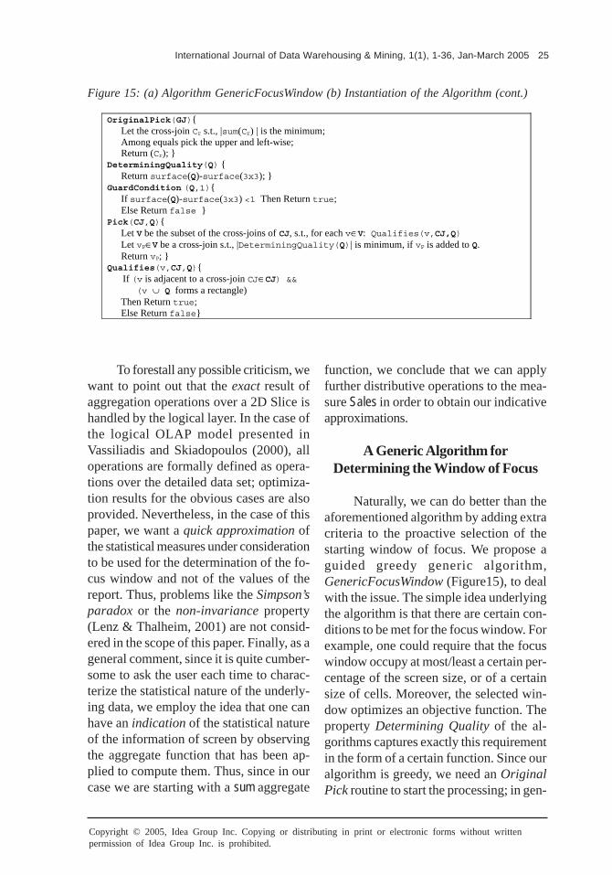
Algorithm GenericFocusWindow Input:

A set of cross-joins GJ and a display grid of cells Grid related to GJ. Each cell belonging to Grid is characterized by coordinates (x,y) and each CJ belonging to GJ is

characterized by the coordinates of its upper left and lower right cell. Each cross-join has a surface, determined by its coordinates.

Parameters: OriginalPick(GJ): a routine to determine the starting cross-join of the algorithm GuardCondition: a routine to determine whether the algorithm should stop 4: a tolerance or error range for the acceptance of a solution or not Qualifies: a Boolean function that determines whether a solution satisfies a set of constraints DeterminingQuality: a property of a cross-join like surface, sum of values, … Pick(GJ,Q): a routine picking a cross-join to enlarge the produced solution

Output:

A set of cross-joins, Q that satisfies the conditions set by the user.

Begin

1.1. Q = {} 1.2. C = OriginalPick(GJ)

Add C to Q. While (GuardCondition) { CJ = Pick(GJ,Q); If CJ≠NULL Then add CJ to Q Else exit the loop } Return Q

End.

Figure 15: (a) Algorithm GenericFocusWindow (b) Instantiation of the Algorithm



To forestall any possible criticism, wewant to point out that the exact result ofaggregation operations over a 2D Slice ishandled by the logical layer. In the case ofthe logical OLAP model presented inVassiliadis and Skiadopoulos (2000), alloperations are formally defined as opera-tions over the detailed data set; optimiza-tion results for the obvious cases are alsoprovided. Nevertheless, in the case of thispaper, we want a quick approximation ofthe statistical measures under considerationto be used for the determination of the fo-cus window and not of the values of thereport. Thus, problems like the Simpson’sparadox or the non-invariance property(Lenz & Thalheim, 2001) are not consid-ered in the scope of this paper. Finally, as ageneral comment, since it is quite cumber-some to ask the user each time to charac-terize the statistical nature of the underly-ing data, we employ the idea that one canhave an indication of the statistical natureof the information of screen by observingthe aggregate function that has been ap-plied to compute them. Thus, since in ourcase we are starting with a sum aggregate

function, we conclude that we can applyfurther distributive operations to the mea-sure Sales in order to obtain our indicativeapproximations.

A Generic Algorithm forDetermining the Window of Focus

Naturally, we can do better than theaforementioned algorithm by adding extracriteria to the proactive selection of thestarting window of focus. We propose aguided greedy generic algorithm,GenericFocusWindow (Figure15), to dealwith the issue. The simple idea underlyingthe algorithm is that there are certain con-ditions to be met for the focus window. Forexample, one could require that the focuswindow occupy at most/least a certain per-centage of the screen size, or of a certainsize of cells. Moreover, the selected win-dow optimizes an objective function. Theproperty Determining Quality of the al-gorithms captures exactly this requirementin the form of a certain function. Since ouralgorithm is greedy, we need an OriginalPick routine to start the processing; in gen-

OriginalPick(GJ){ Let the cross-join Cr s.t., |sum(Cr) | is the minimum; Among equals pick the upper and left-wise; Return (Cr); } DeterminingQuality(Q) { Return surface(Q)-surface(3x3); } GuardCondition (Q,1){ If surface(Q)-surface(3x3) <1 Then Return true; Else Return false } Pick(CJ,Q){ Let V be the subset of the cross-joins of CJ, s.t., for each v∈V: Qualifies(v,CJ,Q) Let vP∈V be a cross-join s.t., |DeterminingQuality(Q)| is minimum, if vP is added to Q. Return vP; } Qualifies(v,CJ,Q){ If (v is adjacent to a cross-join CJ∈CJ) && (v ∪ Q forms a rectangle) Then Return true; Else Return false}

Figure 15: (a) Algorithm GenericFocusWindow (b) Instantiation of the Algorithm (cont.)



eral this is closely related to the Determin-ing Quality function and we require that itstart with a smallest value. Moreover, aGuard Condition checks for the satisfac-tion of the desired property, meaning thatwe can possibly allow a certain approxi-mation error ε to out obtained solution. Fi-nally, a function Pick provides the neces-sary details for working from the originalsmall-in-value solution towards the finalresult, practically picking the next cross-join to enlarge the current window of fo-cus.

One implicit assumption that our al-gorithm makes is that the Original Pickfits inside the allowed window. This con-straint can easily be relaxed by an exten-sion of the algorithm picking subparts of across-join in a similar fashion with the pro-posed algorithm, if we consider that we picksubparts of a 2D-slice.

We present an example for theinstantiation of the aforementioned genericalgorithm in Figure 15b, where we are in-terested in a focus window which (a) in-cludes the window with the minimum sum-mary of values and (b) is not bigger than3x3 (with a tolerance of the surface ε=1).

To accomplish this, we initialize accordinglythe parameters of the algorithm(GuardCondition, ε) and define accordinglythe functions of the algorithms (OriginalPick,DeterminingQuality and Pick). The greedyalgorithm is guided to pick the window ofminimum value as its starting point. Thefirst constraint is met by the original pickand the second by the stop condition of thealgorithm. During the expansion phase,each time we choose a cross-join such that(a) is neighbouring with the current solu-tion; (b) if merged with the current solu-tion, it comprises a rectangle (easily deter-mined by comparing the lengths of the op-posite sides of the new solution; and (c)has the smallest surface.

If we execute the algorithm on thedata of Figure14, the result will be Q={R1/C6,R2/C6,R3/C6,R4/C6}, which is practicallythe tape C6. If, instead of the minimumvalue, in function Pick we had chosen themaximum, then the result would be Q={R1/C6,R1/C5}. Another obvious extensionwould be to employ a 2-greedy algorithm:in this case the small cross-joins R2/C5 andR2/C6, each comprising a single cell, couldhave been incorporated in the solution, too.

��

��

��

��

�

��

�

��

��

��

��

�

��

�

�

��

��

��

��

�

��

��

��

�

�

�

��

��

��

�

��

�!

��

�

��

"�

��

Local StorageCaching

"�� # �$ �� %�"�# �$ ��

OLAP ServerOLAP Server�

Focus + Context

Figure 16: The System Architecture of CubeView



In Maniatis et al. (2003a), we presentmore examples for the instantiation of thealgorithm.

IMPLEMENTATION

In this section we will present aframework in support of Mobile OLAP, aterm used to express the porting of require-ments and specifications for OLAP appli-cations into the wireless and mobile com-puting world, as introduced in Maniatis(2004). In this context, we presentCubeView, a pilot academic platform en-abling OLAP visualization both for contem-porary desktops as well as for mobile de-vices. We present details about the adoptedsystem and software architecture of thesystem, along with explanations on the us-age of the system.

The Architecture of CubeView

In this section we present the archi-tecture of CubeView, organized as (a) sys-tem architecture, (b) software architecture,and (c) implementations specifics.

The system architecture forCubeView is depicted in Figure16. Thegeneral idea is that the user on the mobiledevice (PDA, mobile phone, or even re-mote desktop PC) uses a specific user in-terface on the user’s device to navigate onthe screen between OLAP data and per-form OLAP analysis in general, based ondata stored locally on the device in highlyaggregated and summarized format.

The system is composed of three dis-crete and autonomous modules: A tradi-tional OLAP Server Module, used as ablack box in the process since it can beany of the existing commercial, open source,or academic ones; a Middleware Appli-cation Server, serving as the mediator be-

tween the data stored in the OLAP Serverand the mobile device and the mobileFront-End Applications, incorporating thelocal storage; and the user interface, navi-gation, and presentation options.

The Software Architecture ofCubeView is depicted in Figure17. Eachdistinct system layer holds a number ofsoftware modules, each in turn performingspecific tasks in the context of the wholesystem. To be more specific, the softwarelayers of CubeView are:• The OLAP Server Layer, which, as

mentioned before, is “transparent” to theuser and used as a “black box” fromthe system, meaning that only a specificAPI is used to query the server forOLAP data. Typically, any availableOLAP server (MOLAP or ROLAP),commercial, or academic platform couldbe used for storing and processing theactual OLAP queries.

• The Application Server Layer, whichis the software layer holding the Javaserver-side application logic. It incorpo-rates the following software modules: (i)The Query Manager, responsible fordirectly querying the OLAP Server ac-cording to the query posed by the mo-bile user; (ii) the XML OLAP DataManager, a component responsible forformatting the requested data in XMLformat and interacts with (iii) the Cubeto CMP (XML) Converter; and (iv) theXML Cross-join Metadata, which for-mats the OLAP data queried in a for-mat suitable for presentation using CPMentities. A simple (v) Caching Mecha-nism is employed for performance pur-poses, which holds both the actual OLAPdata and the necessary OLAPmetadata, retrieved and managedthrough (vi) the OLAP Metadata Man-ager. Finally, (vii) the Connection Man-



ager is the synchronization mediatorbetween the Application Server and theUser Layer, controlling the connectionprocess when data from the OLAPServer are needed to refresh the OLAPdata in CPM entities format, stored lo-cally on the mobile device.

• The User Layer incorporates a numberof software modules and client tools thatsupplies the mobile user with instrumentsfor (i) storing OLAP data locally on theLocal Storage RDBMS, which holds themetadata of the system as well as highlyaggregated OLAP data; (ii) executing

Figure 17: The Software Architecture of CubeView

Figure 18: A Prototype Front-End for CubeView on Pocket PC Employing OLAP Lens



simple ad hoc local queries, meaning onthe OLAP data stored locally through(iii) the OLAP Query Manager; (iv)the OLAP Request Manager interactswith the Application Server Layer —actually with the Connection Manager— to retrieve data from the OLAPServer if such a case is enforced due tothe query posed by the user; and finally,(v) a suitable User Interface and Lo-cal Metadata Browser are the front endtools on the mobile device through whichthe user can pose queries, browse thelocal data, and display the results of hisqueries on OLAP screens, employing theTable Lens visualization technique.

Using CubeView

In this section we give an illustrativeexample of how CubeView is designed towork and respond to queries posed by mo-bile users.

An implementation on a Pocket PCenvironment of the example described inFigure 2 is displayed in Figure 18, where aprototype for the front end tool used is de-veloped and displayed on the simulator pro-vided by Microsoft (http://www.microsoft.com/windowsmobile / informat ion/devprograms/default.mspx). In terms ofusability of the system and user interfacecharacteristics, special features are em-ployed. A step-by-step usability of the userinterface controls is as follows:• The user exploits the user interface fa-

cilities of the front end application tospecify the user’s range query, usingdrag and drop to select from the pop updimensions window the actual dimensionlevels to form the initial screen. The firstlevel of the highly aggregated data ap-pears on the screen (Figure 18).

• In a next specialization manipulation, theuser selects from a pop up menu a func-tion or formula (system or user defined)

Figure 19: OLAP Lens User Interface Details



to focus on specific characteristics andattributes of the displayed data. For ex-ample, it may be that the user wants tolocate the cell with the max value of thedisplayed data and drill into them to lo-cate further details. The appearance ofthe display screen focuses to the desiredcell, which is distorted (in accordanceto the Table Lens characteristics) toguide the user to the exact results of theuser’s query (Figure 19).

• By double clicking on the focused cell,the user drills in to the details of the cell.The cross tab displayed is replaced bythe next level of the dimension hierar-chies, both for rows and columns. Theprevious level of the dimension hierar-chies is displayed as pull down menuson the top of the screen.

• The user may continue performing theprevious steps to perform further analy-sis. Special controls (such as �� fordrill in and drill out) and menu optionsassist the user in performing OLAPanalysis on the user’s mobile device.

Finally, we would also like to point outthat the architecture implemented inCubeView is flexible enough to provide aframework suitable for both desktop andmobile OLAP visualization applications.

RELATED WORK

In this section, we will present relatedwork on the topics covered by our research.This includes existing presentation modelsfor databases and multidimensional data,implementations of visualization tools, anda discussion of related efforts in the fieldof OLAP for mobile environments.

Furthermore, we should mention thatpreliminary results of the work analysedherein can be found in Maniatis et al. (2003),

Maniatis et al. (2003a), Maniatis (2003),and Maniatis (2004). Still, in this paper, (a)we provide the big picture for these works,(b) we have further decoupled the logicaland presentational models from the workof Maniatis et al. (2003), and (c) we pro-vide more examples and details on theproofs.

Presentational Models

Although OLAP has been an activeresearch area for the past few years, theefforts devoted to the visualization ofOLAP screens are very scarce. To ourknowledge, only two such efforts exist.

The first effort is from the industrialfield, where Microsoft has issued a com-mercial standard for multidimensional da-tabases and where the presentational is-sues form a major part (Microsoft, 1998).In this approach, a powerful query languageis used to provide the user with complexreports created from several cubes (or ac-tually subsets of existing cubes). However,this standard suffers from several problems,with two of them being the most promi-nent: First, the logical and presentationalmodels are mixed, resulting in a complexlanguage that we personally found hard touse (although powerful enough). Secondly,the model is formalized but not thoroughly;for instance, we did not really see a defini-tion for the schema of a multicube. Also,there are specific axes that are predefined,namely “rows,” “columns,” “pages,” “sec-tions,” and “chapters”; no other axes aresupposed.

The second proposal is an academicapproach — the Tape Model (Gebhardt etal., 1997) — based on the notion of“Tapes,” called thus due to their look andfeel. Tapes are infinite and can overlap (ifthey contain shared data dimensions) orintersect with each other. A two-dimen-



sional intersection is called a matrix andrepresents a kind of cross-tab between thecorresponding dimensions. Each tape com-prises a variable number of tracks. Themost important operations on tapes include:(a) insertion and deletion of tracks; (b)changing the sequence of tracks (e.g., sort-ing); and (c) scrolling on tracks. The modeloffers the possibility of defining hierarchi-cal structures within a tape. Tapes are infi-nite and can overlap (if they contain shareddata dimensions) or intersect with eachother. A two-dimensional intersection iscalled a matrix and represents a kind ofcross-tab between the corresponding di-mensions. Each tape comprises of a vari-able number of tracks.

Compared to CPM, the aforemen-tioned models can be characterized as fol-lows: CPM is a formal approach, with arigorous formal background. The tapemodel seems to be limited in its expressivepower (with respect to the Microsoft pro-posal), and, to our knowledge, its formalaspects are not yet publicly available. TheMicrosoft proposal, on the other hand, ap-pears to be too complicated, without a clean-cut separation of the underlying concepts.Also, its coupling to the underlying logicalstructures is not clear.

Visualization in ContemporaryOLAP Tools

Most vendors offering data ware-housing and OLAP tools and platformshave included in their products special mod-ules running on mobile devices and offer-ing OLAP analysis possibilities to mobiledecision makers. Vendors such asMicroStrategy Inc. (http://www.microstrategy.com) and Business Objects (http://www.businessobjects.com) have done agreat deal towards implementing dedicated

broadcast servers that provide OLAP spe-cific information to users in numerous typi-cal formats such as e-mails, beeps on pag-ers, or specifically designed Web pages,using WAP and WML and employing aspecific but typical server-based architec-ture to offer this functionality.

With respect to academic pilot visu-alization tools and platforms, numerous havebeen developed, mainly in the area of thegeneral area of information visualization.Many proposals focused on more specificareas such as statistical and scientific da-tabases, data mining, and multidimensionaldata visualization. In the last area, we canmention VisDB (Keim & Kriegel, 1994),HD-Eye (Hinneburg et al., 2002) and Po-laris (Stolte & Hanrahan, 2000).

VisDB (Keim & Kriegel, 1994) andits more recent sibling HD-Eye (Hinneburget al., 2002) originated from the area ofgeneral database exploration techniques,with specialization in multi-dimensional vi-sualization. It cannot be considered as anOLAP visualization platform; instead, it isa platform for the exploration of large multi-dimensional data sets using techniques suchas the mapping of two dimensions toaxes, parallel coordinates, etc., all inte-grated into an interactive graphical en-vironment. In a sense, ViSDB can beviewed as being closer to data miningthan OLAP. HD-Eye is a more recentversion oriented towards visual cluster-ing of large data sets containing high-dimensional data.

Finally, Polaris (Stolte & Hanrahan,2000) is one of the most recently designedand implemented visual interfaces, designedto explore large multi-dimensional data-bases that extends the well-known PivotTable interface. The features of Polarisinclude an interface for constructing visualspecifications of table-based graphical dis-



plays and the ability to generate a preciseset of relational queries from the visualspecification. The visual specifications canbe incrementally developed, giving the ana-lyst visual feedback as they construct com-plex queries and visualizations.

Applications for Mobile OLAP

OLAP-specific functionality for mo-bile devices provided by the vendors doesvery little towards exploiting the specificcharacteristics and power of the mobiledevices on which these applications run.Rather, they base their solutions on migrat-ing the desktop OLAP interface of theirtools to the mobile device employing WAPand the WML, but fail to take into accountrecent improved facts about mobile devicessuch as increased system memory; clearercolor screens; increased processing poweror their limitations, such as small screensize, different usability, and user interfacerequirements; common off line work, etc.

To fill this gap, numerous approachescoming mainly from the academia and fromvarious research areas have been propos-ing solutions and frameworks that addressthis problem. Many of them propose novelapproaches to cope with the case of mo-bile OLAP and, more importantly, many ofthem have been actually implemented andused in real case scenarios. We will brieflypresent some of the most notable (in ourjudgment) approaches.

MOCHA (Rodriguez-Martinez &Rossopoulos, 2000) was an early, moregeneric approach to a database middlewarefor distributed data sources, which, althoughnot specifically addressing the case of mo-bile devices and OLAP, incorporates manyof the notions present in “Mobile OLAP,”such as the distributed nature of the sys-tem, the scaling to a larger environment,

and the novel approach of deploying appli-cation-specific functionality from one pointof the system to all the others through themiddleware itself. The system was imple-mented in Java, which allowed for the ship-ping of Java code to implement either ad-vanced data types or tailored remote op-erators to remote data sources and have itexecuted remotely, and was actually put towork effectively on a large aerospace or-ganization.

A more specific approach is pre-sented in Cuzzocrea et al. (2003), namelyHand-OLAP, a system specifically de-signed for bringing OLAP functionality tousers of mobile devices. This proposal fo-cuses mainly on a number of the draw-backs of handhelds devices, with empha-sis on the small storage space and the usualdiscontinuance of the connection to theWireless LAN, as opposed to the userneeds for querying and browsing informa-tion extracted from enormous amounts ofdata accessible through the network. Tocope with this issue, this approach focuseson presenting a solution for storing locallyin the mobile device a compressed andhighly summarized view of the data thatcan be more efficiently transmitted fromthe OLAP server than the original ones.Hand-OLAP is a prototype system with asuitable architecture that seamlessly sup-ports the interaction between mobile de-vice and OLAP server, stores data locallyon the mobile device in a compressed for-mat (based on Quadtree representation),and always provides the user with a spe-cific bi-dimensional (tabular) view of thedata, even when the connection to theWLAN is off.

Finally, the work of Sharaf andChrysanthis (2002, 2002a) focused moreon matters of wireless network and powerconsumption on the mobile devices, pro-



posing a suitable mobile OLAP model, alongwith an on-demand scheduling algorithm tominimize access time and energy consump-tion on mobile agents. This approach isbased also on summary tables, along withthe functionality of simple OLAP front-endtools to execute simple SQL queries. Whatis more, this proposal maximizes the ag-gregated data sharing between clients andreduces the broadcast length. Finally, theproposed on-demand scheduling algorithmemploys user parameters to fine tune thedegree of aggregation of data so as to con-trol the tradeoff between access time andenergy consumption, and adapts to differ-ent request rates, access patterns, and datadistributions.

As a whole, as we compareCubeView with all the previously describedtools — those used for visualization andthose reviewed for Mobile OLAP — westress the fact that our prototype is the onlyone that supports the full cycle, starting froma formal and rigorous theory backgrounddepicted in CPM itself, and reaching a fullfledged implementation covering bothworlds, the traditional desktop environ-ments, and the mobile devices. All the otherparadigms are departmental in the sensethat the they tamper only portions of thebig picture, this being either the informa-tion visualization area (VisDB [Keim &Kriegel, 1994]; HD-Eye [Hinneburg et al.,2002]; Polaris [Stolte & Hanrahan, 2000]),or specific approaches and implementa-tions for mobile devices (Hand-OLAP[Cuzzocrea et al., 2003]) or simplymiddleware, like MOCHA (Rodriguez-Martinez & Rossopoulos, 2000), or, finally,a framework for a wireless OLAP model(Sharaf & Chrysanthis, 2002, Sharaf &Chrysanthis, 2002a).

CONCLUSIONS &FUTURE WORK

So far, visualization has not been fullyincorporated in the abstraction levels ofDBMS architecture (conceptual, logical, orphysical). In this paper, we have discussedthe separation of the aforementioned ab-straction levels to take visualization intoconsideration. In this context, we have pre-sented the Cube Presentation Model(CPM), a formal presentation model forOLAP data. Our contributions can be listedas follows: (a) we have presented an ex-tension of a previous logical model forcubes to handle more complex cases; (b)we have introduced a novel presentationalmodel for OLAP screens, intuitively basedon the geometrical representation of a cubeand its human perception in the space; and(c) we have discussed how these two mod-els can be smoothly integrated. Moreover,we have demonstrated how CPM can benaturally mapped into an advanced visual-ization technique (Table Lens), and we havediscussed suitable algorithms for proactiveautomated support of the user towards thehighlighting of interesting areas of a report.Finally, we have discussed implementationand usage issues in the context of an aca-demic prototype system (CubeView) thatwe have implemented.

Obviously, we do not claim that thisis the ultimate solution to the problem ofOLAP data visualization, but rather we wishto indicate that there is quite an interestingresearch field in this area and a supportivebody of knowledge from other disciplinessuch as Human-Computer Interaction andInformation Visualization.

An obvious particularity of our ap-proach is that it is crafted mostly for tabu-lar data in the context of OLAP. Should



we wish to differentiate the context of datautilization or the data themselves (e.g., per-form OLAP over spatial or biological data),the presentation and visualization techniqueswould have been different. In general, it isan interesting research challenge to discussthe integration of different models in thepresence of different contexts, either interms of the data or their usage.

At the same time, new hardware de-velopments pose new requirements for ourvisualization techniques. One of our goalshas been to implement OLAP visualizationtechniques for particularly small devicessuch mobile phones and palmtops. Althoughthe processing power of these gadgets isno more negligible (actually, the buzzword“thin client” seems to disappear from thestandard vocabulary of the area), theirscreen sizes shrink over time. To makeOLAP screens presentable to such de-vices, one can follow several paths suchas: (a) showing only high level summarieswhich involve small 2D slices or (b) show-ing simply pie or bar charts. We have cho-sen an alternative approach where (a) thecontents of the screen do not have to besqueezed in size in order to fit in the screen,and, most importantly, (b) the report doesnot have to be rewritten and neither do wehave to check for the aggregation level ofthe presented data. On the contrary, a cer-tain part of the report is presented, depend-ing on the particularities of the device. Here,we make the reasonable assumption thateither the device has the computationalpower to determine the amount of cells thatcan be presented to the user, or, if this isnot an option, the device can at least piggy-back its characteristics to the OLAP serverand let the server decide on the focus win-dow. Naturally, as part of future research,different implementation issues (e.g., cach-ing schemes or visualization techniques) canbe applied in this context.

Finally, coming back to the visualiza-tion issue, we have brought up Table Lensto highlight the possibility of facilitating pro-active user decision support in the pres-ence of large datasets (in our case, thevalue axis is quite larger than the size thatsomeone can handle efficiently). Clearly,as report screens are limited, not only dueto hardware constraints but also due to theparticularities of human nature (e.g., theclassical discussion on the limited capacityof persons in processing information (Miller,1956), it comes quite natural that automatedproactive support to the users is thus oneof the new requirements that decision sup-port tools have to provide. Thus, our con-tribution is related to a broader line of re-search (Han, 1998, Sarawagi et al., 1998),which is obviously open to a wide range ofdifferent possibilities.

REFERENCES

Abiteboul, S. et al. (2003). The Lowell da-tabase research self assessment. Re-trieved from: http://research.microsoft.com/~Gray/lowell/

Cuzzocrea, A., Furfaro, F., & Sacca, D.(2003, April 9-11). Hand-OLAP: A sys-tem for delivering OLAP services onhandheld devices. In Proceedings ofISADS 2003. Pisa, Italy, (pp. 213-224).

Gebhardt, M., Jarke, M., & Jacobs, S.(1997). A toolkit for negotiation supportinterfaces to multi-dimensional data. InProceedings of ACM SIGMOD 1997(pp. 348-356).

Han, J. (1998). Towards on-line analyticalmining in large databases. SIGMODRecord, 27(1), 97-107.

Hinneburg, A., Keim, D.A., & Wawryniuk,M. (2002). HD-eye: Visual clustering ofhigh-dimensional data. In Proceedingsof the 2002 ACM SIGMOD 2002.Madison, Wisconsin, p. 629.



Inmon, W.H. (1996). Building the DataWarehouse. John Wiley & Sons.

Inselberg, A. (2001). Visualization andknowledge discovery for high dimen-sional data. The Second Workshop Pro-ceedings of UIDIS. IEEE Press.

Keim, D.A. (1997). Visual data mining.Tutorials of the 23rd International Con-ference on Very Large Data Bases. Ath-ens, Greece.

Keim, D.A. & Kriegel, H.P. (1994): VisDB:Database exploration using multidimen-sional visualization. IEEE ComputerGraphics and Applications, Septem-ber.

Kimbal, R., Reeves, L., Ross, M., &Thornthwaite, W. (1998). The DataWarehouse Lifecycle Toolkit: ExpertMethods for Designing, Developing,and Deploying Data Warehouses. JohnWiley & Sons.

Lenz, H.J. & Thalheim, B. (2001). OLAPdatabases and aggregation functions. InProceedings of the SSDBM 2001.Fairfax, Virginia, (pp. 91-100).

Maniatis, A. (2003). OLAP presentationmodeling with UML and XML. In Pro-ceedings of BCI 2003. Thessaloniki,Greece, (pp. 232-241).

Maniatis, A. (2004). The case for mobileOLAP. Proceedings of the First In-ternational Workshop on PervasiveInformation Management (in conjunc-tion with EDBT ’04). Heraklion, Greece,(pp. 103-114).

Maniatis, A., Vassiliadis, P., Skiadopoulos,S., & Vassiliou, Y. (2003). CPM: A cubepresentation model for OLAP. In Pro-ceedings of DaWaK 2003. Prague,Czech Republic (pp. 4-13).

Maniatis, A., Vassiliadis, P., Skiadopoulos,S., & Vassiliou, Y. (2003a). Advancedvisualization for OLAP. In Proceedingsof DOLAP 2003. New Orleans, Loui-siana (pp. 9-16).

Microsoft (1998). OLEDB for OLAP. Re-trieved from: http://www.microsoft.com/data/oledb/olap/

Miller, G.A. (1956). The magical numberseven, plus or minus two: Some limitson our capacity for processing informa-tion. Psychological Review, 63, 81-97.

Pirollo, P. & Rao, R. (1996). Table lens asa tool for making sense of data. In Pro-ceedings of the AVI 1996 Workshop.Gubbio, Italy.

Rao, R. & Card, S.K. (1994). The tablelens: Merging graphical and symbolicrepresentations in an effective focus +context visualization for tabular informa-tion. In Proceedings of ACM SIGCHI1994. Boston, Massachusetts.

Rodriguez-Martinez, M. & Rossopoulos,N. (2000). MOCHA: A self-extensibledatabase middleware system for distrib-uted data sources. In Proceedings ofACM SIGMOD 2000. Dallas, Texas,(pp. 213-224).

Sarawagi, S., Agrawal, R., & Megiddo, N.(1998). Discovery-driven exploration ofOLAP data cubes. In Proceedings ofEDBT 1998. Valencia, Spain, (pp. 168-182).

Sharaf, M.A. & Chrysanthis, P.K. (2002).On-demand broadcast: New challengesand algorithms. In Proceedings ofHDMS 2002. Athens, Greece.

Sharaf, M.A. & Chrysanthis, P.K. (2002a).Semantic-based delivery of OLAP sum-mary tables in wireless environments.In Proceedings of CIKM 2002.McLean (pp. 84-92).

Stolte, C. & Hanrahan, P. (2000). Polaris:A system for query, analysis and visual-ization of multidimensional relational da-tabases. In Proceedings of InfoVis2000. Salt Lake City, Utah, (pp. 5-14).

Tsois, A., Karayannidis, N., & Sellis, T.(2001). MAC: conceptual data model-ing for OLAP. In Proceedings of



DMDW 2001. Interlaken, Switzerland,(pp. 5.1-5.11).

Vassiliadis, P. & Sellis, T. (1999). A surveyon logical models for OLAP databases.SIGMOD Record, 28(4), 64-69.

Vassiliadis, P. & Skiadopoulos, S. (2000).Modeling and optimization issues for

Andreas Maniatis received his diploma from the National Technical University of Athens and iscurrently a PhD student at the same university. His research lies in the area of databases, andhis main research interests include data warehousing, OLAP, information visualization,pervasive computing, and software engineering. Mr. Maniatis is a member of ACM, IEEE, andthe Technical Chamber of Greece.

Panos Vassiliadis received his diploma and PhD from the National Technical University ofAthens. Dr. Vassiliadis is editor of the book Fundamentals of Data Warehouses (Springer-Verlag). He has more than 25 publications in international refereed journals and conferences.Dr. Vassiliadis has been a program committee member for several conferences and a reviewerfor Information Systems and VLDB Journal. His research lies in the area of databases, and hismain research interests include data warehousing, OLAP, ETL, metadata management and Webservices. Dr. Vassiliadis is a member of ACM, IEEE, and the Technical Chambers of Greece.

Spiros Skiadopoulos received his diploma and PhD from the National Technical University ofAthens and his MSc from UMIST. He has more than 20 publications in international refereedjournals and conferences. Dr. Skiadopoulos has been a reviewer for several conferences andjournals. His research lies in the area of databases, and his main research interests includedata warehousing, OLAP, Spatial Databases, metadata management and Web services. Dr.Skiadopoulos is a member of the American Association for Artificial Intelligence and theTechnical Chamber of Greece.

Yannis Vassiliou is a professor at the National Technical University of Athens, School of Electricaland Computer Engineering since 1992. Before that he was a professor at New York Universityand the University of Crete. He is a member of the Scientific Council of the Greek Parliament.He has been project director and researcher in numerous competitive research projects and isthe author of more than 100 scientific articles. His main research interests are in databases,data warehouses, e-Business and enterprise information systems.

George Mavrogonatos is a senior student at the Electrical and Computer Engineering Schoolat the National Technical University of Athens.

Ilias Michalarias is a senior student at the Electrical and Computers Engineering School atthe National Technical University of Athens.

multidimensional databases. In Pro-ceedings of CaiSE 2000. Stockholm,Sweden, (pp. 482-497).

a presentation model & non-traditional visualization for...

Documents