a pretest for choosing between logrank and wilcoxon … · a pretest for choosing between logrank...

METRON - International Journal of Statistics2010, vol. LXVIII, n. 2, pp. 111-125

RUVIE LOU MARIA C. MARTINEZ – JOSHUA D. NARANJO

A pretest for choosing between logrankand wilcoxon tests in the two-sample problem

Summary - Two commonly used tests for comparison of survival curves are the gen-eralized Wilcoxon procedure of Gehan (1965) and Breslow (1970) and the logranktest proposed by Mantel (1966) and Cox (1972). In applications, the logrank test isoften used after checking for validity of the proportional hazards (PH) assumption,with Wilcoxon being the fallback method when the PH assumption fails.

However, the relative performance of the two procedures depend not just on thePH assumption but also on the pattern of differences between the two survival curves.We show that the crucial factor is whether the differences tend to occur early or latein time. We propose diagnostics to measure early-or-late differences between twosurvival curves. We propose a pretest that will help the user choose the more efficienttest under various patterns of treatment differences.

Key Words - Logrank; Wilcoxon; Pretest; Proportional hazards; Lehmann alternative.

1. Introduction

In survival analysis, treatment efficacy is often analyzed by comparingthe survival rates of two treatment groups. Two commonly used tests for thecomparison of survival distributions are the generalized Wilcoxon procedure(Gehan, 1965; Prentice, 1978) and the logrank test (Mantel, 1966; Cox, 1972;Peto and Peto, 1972). Both tests are based on the ranks of the observations,and have several versions in the literature. In this paper, the Wilcoxon testwill refer to the approximation by Prentice (1978) of the statistic proposed byGehan (1965). The logrank test will refer to the Peto and Peto (1972) versionof the statistic proposed by Mantel (1966). Leton and Zuluaga (2005) presenta comprehensive summary of the different names, versions and representationsof the generalized Wilcoxon and logrank tests.

The finite sample performance of these tests have been compared in severalsimulation studies. Lee, Desu, and Gehan (1975) compared size and power of

Received March 2008 and revised June 2010.

112 RUVIE LOU MARIA C. MARTINEZ – JOSHUA D. NARANJO

the tests using small samples from exponential and Weibull survival distributionswith and without censoring. Latta (1981) extended the simulations to includethe lognormal survival distribution, allow for unequal sample sizes, and allowfor censoring in only one sample. Beltangady and Frankowski (1989) focusedon the effect of unequal censoring, using various combinations of censoringproportions. More recently, Leton and Zuluaga (2001, 2005) compare theperformance of various versions of the generalized Wilcoxon and logrank testsunder scenarios of early and late hazard differences.

In general, the logrank test tends to be sensitive to distributional differenceswhich are most evident late in time. In comparison, the Wilcoxon test tendsto be more powerful in detecting differences early in time (Lee, Desu, Gehan,1975; Prentice and Marek, 1979). Lee et al. (1975) have shown that whenthe hazard ratio is nonconstant the generalized Wilcoxon test can be morepowerful than the logrank test. In applications, the logrank test is often usedafter checking for validity of the proportional hazards (PH) assumption, withWilcoxon being the fallback method when the PH assumption fails.

The properties of the logrank test are discussed extensively in the litera-ture (Breslow, 1970; Cox, 1972; Peto, 1972; Peto and Peto, 1972, or see thesummaries in Kalbfleisch and Prentice ,1980; Andersen et al., 1993, and Kleinand Moeschberger, 1997). It is known to be a fully efficient rank test under theproportional hazards assumption, or Lehmann alternative. The Lehmann alter-native describes an exponentiated relationship between the two survival curves,i.e. S2(t) = [S1(t)]

ψ . In the next section we show that when two survivalcurves satisfy the proportional hazards assumption, then Lehmann alternativenecessarily follows.

There have been several graphical methods suggested for assessing theproportional hazards assumption (Hess, 1995). One commonly used graphicalmethod that is available on many statistical software (i.e. SAS, Stata and R)is the plotting of the log of the cumulative hazard function against log timeand checking for parallelism.

We show that it is useful and easy to discriminate based not on the pro-portional hazards assumption, but on whether treatment differences occur earlyor late in the time range of comparison. We propose a pretest for early orlate treatment differences that will help the user choose between the logrankand Wilcoxon tests. Simulation results show that an adaptive test procedureusing the pretest achieves power that is closer to the more powerful test undervarious conditions.

The pretest proposed here is useful only when the survival curves do notcross. When the survival curves cross, both logrank and Wilcoxon tests havelow power, since early differences tend to negate late differences. Therefore, theadaptive test will also have low power. There are specific methods in the litera-ture designed to handle crossing alternatives (see e.g. Stablein and Koutrouvelis

A pretest for choosing between logrank and wilcoxon tests in the two-sample problem 113

(1985), Shen and Le (2000), Bagdonavicius, Levuliene, Nikulin and Zdorova-Cheminade (2004) and Bagdonavicius and Nikulin (2006)). A related issue ofcrossing hazard functions is discussed in Bagdonavicius, Levuliene and Nikulin(2009).

2. Proportional hazards model, Lehmann alternative and the Weibull

distribution

The Cox proportional hazards model (Cox, 1972) can be written as

hi(t |xi1 . . . xip) = h0(t) exp{β1xi1 + β2xi2 + · · · + βpxip}. (1)

where the x-variables are covariates. For the two-sample problem, we let p = 1,and let

xi ={ 0 if ith individual belongs to Group 1

1 if ith individual belongs to Group 2

Thus, the lone covariate x is an indicator for group membership. The hazardfunction for the ith individual is

h(t) = h0(t) exp(βxi) ={ h0(t) if ith individual belongs to Group 1

h0(t)ψ if ith individual belongs to Group 2

where ψ = exp(β). Consequently, the hazard functions for the two groups are:

h1(t) = h0(t)

h2(t) = h0(t)ψ,

so that the relationship between the two hazard functions is,

h2(t) = h1(t)ψ. (2)

Since S(t) = exp{− ∫ t

0 h(u)du}

, then it follows that the two survival curvessatisfy

S2(t) = S1(t)ψ (3)

This is called the Lehmann alternative and is the survival representation ofproportional hazards in the two-sample model.

We will show the relationship between proportional hazards and Weibulldistribution. The Weibull distribution is a continuous probability distributioncharacterized by two parameters, γ and λ, with probability density function

f (t) = λγ (λt)γ−1 exp {−(λt)γ } (4)


for nonnegative values of t . The mean and variance are�(1 + 1/γ )

λand

�(1 + 2/γ ) − [�(1 + 1/γ )]2

λ2, respectively, where �(γ ) = ∫ ∞

0 uγ−1e−udu is the

gamma function. The survival function is S(t) = exp[−(λt)γ ] and the hazardfunction is h(t) = λγ (λt)γ−1.

Since two groups satisfy the proportional hazards assumption wheneverS2(t) = S1(t)ψ , it follows that if S1(t) = exp[−(λ1t)γ1] then

S2(t) = [S1(t)]ψ = exp[−(λ1t)γ1ψ]

= exp[−(λ2t)γ2],

if and only if γ2 = γ1 and λ2 = λ1ψ1/γ1 . Therefore, two Weibull distributions

satisfy the proportional hazards assumption if and only if γ1 = γ2.

3. Power comparison of logrank and Wilcoxon tests

To compare the performance of the logrank and Wilcoxon tests, survivaltimes were generated by computer simulation from Weibull distribution withand without censoring. Fifty survival times are generated for each group withthe same censoring proportion for either group. The censoring proportions usedare 0%, 10% and 20%, respectively. For the sample of censored observations,the assumption was that individuals entered the study at a constant rate in theinterval 0 to T and failed according to an exponential distribution.

Let T1 denote the Group 1 random variable. In all simulation cases, T1

will have mean equal to 100. Let T2 denote the Group 2 random variable. T2

was assigned the following 3 cases of alternative distributions.

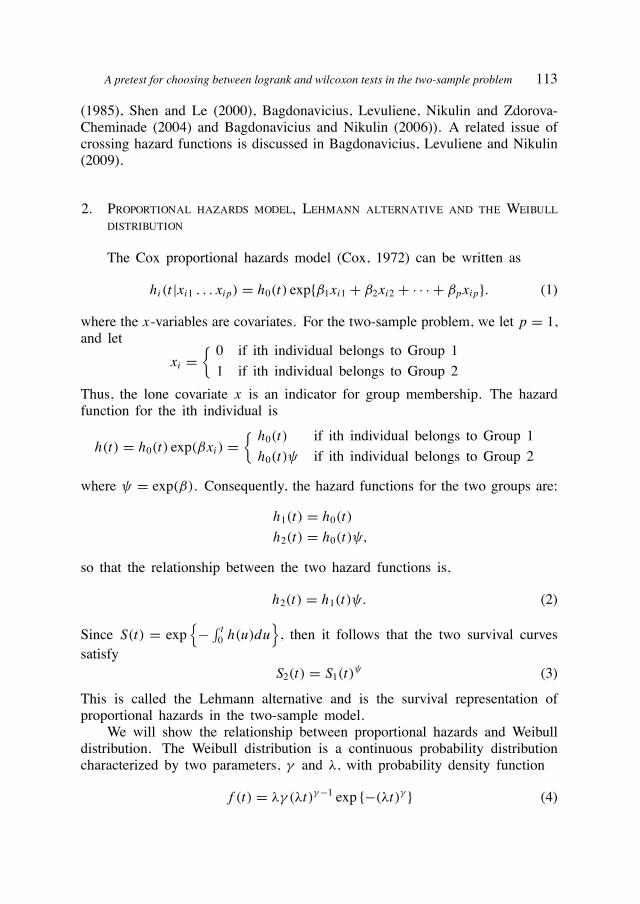
Case 1: T1 ∼ Weibull(γ, λ) and T2 ∼ Weibull(γ, λ/c)This represents the family of alternatives T2 = cT1, where c > 1.Since γ1 = γ2, the proportional hazards assumption is satisfied. Anexample of the survival functions are plotted in Figure 1 with thefollowing parameters T1 ∼ Weibull(γ = 2, λ = 0.0089) and T2 ∼Weibull(γ = 2, λ/c = 0.0063) where c = 1.4.

Case 2: T1 ∼ Weibull(γ, λ) and T2 ∼ Weibull(γ /c, λc)

This represents the family of alternatives T2 = T c1 , where c > 1, or

equivalently log T2 = c log T1, scale transformation in the log scale.Since γ1 �= γ2, the proportional hazards assumption is not satisfied.An example of the survival functions are plotted in Figure 1 withthe following parameters T1 ∼ Weibull(γ = 2, λ = 0.0089) and T2 ∼Weibull(γ /c = 1.8868, λc = 0.0067) where c = 1.06.


Case 3: T1 ∼ Weibull(γ1, λ1) and T2 ∼ Weibull(γ2, λ2), where γ1 < γ2 andλ1 > λ2

This represents a more general family of alternatives than Case 1 orCase 2. For instance, this allows us to choose γ2 and λ2 to achieveearly separation of survival curves. In Figure 1 an example of thesurvival functions are plotted with the following parameters T1 ∼Weibull(γ1 = 2, λ1 = 0.0089) and T2 ∼ Weibull(γ2 = 3, λ2 = 0.0069).

Simulation were done 10,000 times for each case to compare the size andpower of the logrank and Wilcoxon tests. In each case, we used the one-sidedalternative hypothesis that treatment group survival rate is higher than controlgroup.

Since the proportional hazards assumption is satisfied under Case 1, thelogrank test is expected to have higher power than the Wilcoxon test. This isconfirmed by our simulation results (see Table 1). On the other hand propor-tional hazards assumption is not satisfied for Cases 2 and 3 therefore logranktest is not expected to perform well. Our simulation show that the Wilcoxontest outperforms the logrank test in Case 3 (see Table 3), but not in Case 2(see Table 2). Even though Case 2 and Case 3 both violate the proportionalhazards assumption, their type of violation is different. The plot of Case 2 inFigure 1 shows that the separation between the two survival curves occurs laterin time. In contrast, the plot for Case 3 shows that the two survival curvesseparate earlier in time.

The lesson here is to detect not just whether proportional hazards assump-tion is violated, but how it is violated. This suggests diagnostics to detectwhether separation between the two curves is early or late.

4. Lehmann alternative and early-late treatment differences

In this section, we show that proportional hazards in the the two-sampleproblem implies late separation between the two curves.

Lemma 4.1 (Late Treatment Differences). Under the Lehmann alternative (3),the maximum difference between the survival functions S1(t) and S2(t) will occurat t such that S1(t) < 0.4.

Proof. Without loss of generality, let 0 < ψ < 1. Let,

S2(t) − S1(t) = [S1(t)]ψ − S1(t)

= pψ − p

f (p) = pψ − p

where p = S1(t).


The first and second derivatives are,

d

dp

[pψ − p

]= ψpψ−1 − 1 (5)

d2

dp2

[pψ − p

]= ψ(ψ − 1)pψ−2. (6)

Figure 1. Survival plots of T1 ∼Weibull(γ = 2, λ = 0.0089) (©) against various alternative distributions(�).


Table 1: Case 1: Power for the tests in samples of size n1 = n2 = 50 from a Weibull distributionwith equal shape parameters (γ = 2) and treatment effect T2 = cT1.

No censoring 10% censoring 20% censoring

c μ2 − μ1 L W L W L W

1.00 0 0.0496 0.0481 0.0515 0.0487 0.0558 0.0521

1.10 10 0.1582 0.1266 0.1432 0.1269 0.1276 0.1131

1.20 20 0.4301 0.3364 0.3981 0.3310 0.3332 0.2938

1.30 30 0.7341 0.6224 0.6478 0.5610 0.5540 0.5006

L - logrank test; W - Wilcoxon test.

Table 2: Case 2: Power for the tests in samples of size n1 = n2 = 50 from a Weibull distributionwith control group parameters (γ = 2, λ = 0.008862) and treatment effect T2 = T c

1 .


c μ2 − μ1 L W L W L W

1.00 0 0.0506 0.0494 0.0523 0.0496 0.0536 0.0501

1.02 10 0.1610 0.1207 0.1483 0.1196 0.1318 0.1083

1.04 21 0.4625 0.3379 0.4286 0.3188 0.3440 0.2786

1.06 33 0.7937 0.6250 0.7370 0.6009 0.6117 0.5078


Table 3: Case 3: Power for the tests in samples of size n1 = n2 = 50 from a Weibull distributionwith shape parameters γ1 = 2 and γ2 = 3 for Control group and Treatment group, respectively.


μ2 − μ1 L W L W L W

0 0.0496 0.0481 0.0545 0.0509 0.0520 0.0497

10 0.0673 0.2771 0.0790 0.2706 0.0715 0.2370

20 0.2844 0.6179 0.2955 0.5974 0.2594 0.5236

30 0.6360 0.8761 0.5878 0.8366 0.5277 0.7762


The second derivative will always be negative since ψpψ−2 is positive and(ψ − 1) is negative for 0 < ψ < 1. This implies that the function is concavedown and from the first derivative the maximum value of p was computed tobe

S1(t) = p =[

1

ψ

]1/(ψ−1)

(7)

For example, if ψ = 0.5, then S2(t) − S1(t) = [S1(t)]ψ − S1(t) is largest at

S1(t) =(

10.5

)1/(0.5−1) = 0.25. If ψ = 0.80, the maximum difference between


the two curves occurs at S1 =(

10.8

)1/(0.8−1) = 0.3277. We computed thelocation of maximum difference between the two curves for different valuesof ψ . The values are given in Table 4. Observe that the maximum differenceoccur at later times, late enough so that S1(t) < 0.4.

Table 4: Different values of ψ and the corresponding S1(t).

ψ Maximum difference [S1(t)]ψ − S1(t)

achieved at S1(t) equal to

0.10 0.0774

0.20 0.1337

0.30 0.1791

0.40 0.2172

0.50 0.2500

0.60 0.2789

0.70 0.3046

0.80 0.3277

0.90 0.3487

0.99 0.3660

5. Diagnostic for early versus late treatment. Differences: Q Test

Our simulation results show that power performance of logrank test com-pared to Wilcoxon test depends not on proportional hazards assumption butrather on the lateness of separation of survival curves. In this section, wepropose statistics that measure lateness of maximum separation.

Since the values of S1(t) that achieve the maximum separation under theLehmann-alternative are less than 0.4, we measured the degree of separationbefore and after 0.4, for example at 0.2 and 0.6.Let,

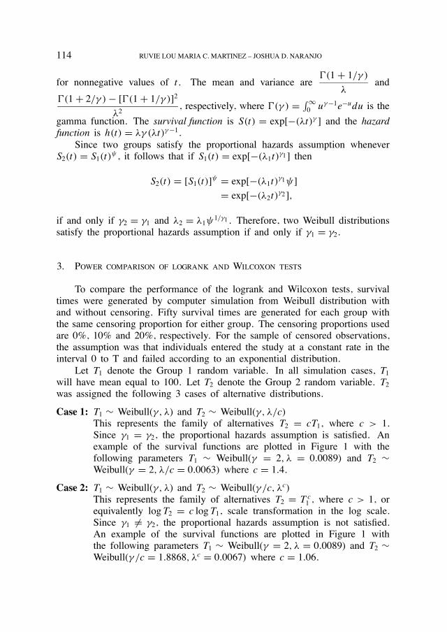
Q = [S̃2(t0.6,1) − S̃1(t0.6,1)] − [S̃2(t0.2,1) − S̃1(t0.2,1)] (8)

wheret0.6, 1 is the time in Group 1 with S̃1(t) = 0.6,

t0.2, 1 is the time in Group 1 with S̃1(t) = 0.2,

S̃2(t0.6, 1) is the survival estimate of t0.6, 1 in Group 2, and

S̃2(t0.2, 1) is the survival estimate of t0.2, 1 in Group 2


Figure 2. Q test on survival functions: ©, Control Group; �, Treatment Group.

If the maximum separation occurs late, the difference S̃2(t0.2,1)− S̃1(t0.2,1) shouldbe larger than S̃2(t0.6,1) − S̃1(t0.6,1) (see Figure 2) and Q will be negative.

In contrast, if separation is early, then we expect Q to be positive. Wepropose an adaptive testing procedure based on Q as follows:

If Q < 0, then use logrank test. Otherwise, use Wilcoxon test. (9)

The theorem below shows that Q < 0 under the Lehmann alternative.

Theorem 5.1. If S2(t) = [S1(t)]ψ , then Q < 0.

Proof. If S2(t) = [S1(t)]ψ , then

Q = [S2(S−11 (0.6)) − 0.6] − [S2(S−1

1 (0.2)) − 0.2]

= [[S1(S−11 (0.6))]ψ − 0.6] − [[S1(S−1

1 (0.2))]ψ − 0.2]

= [(0.6)ψ − 0.6] − [(0.2)ψ − 0.2]

Therefore Q < 0 if

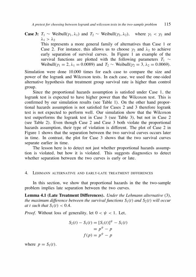
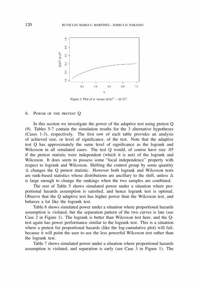
[(0.6)ψ − (0.2)ψ ] < 0.4 (10)

The plot in Figure 3 shows that (10) is satisfied for all ψ < 1.This theorem says that the Lehmann alternative implies Q < 0. Since pro-

portional hazards assumption implies the Lehmann alternative, the proportionalhazards assumption implies Q < 0.


Figure 3. Plot of ψ versus (0.6)ψ − (0.2)ψ .

6. Power of the pretest Q

In this section we investigate the power of the adaptive test using pretest Q(9). Tables 5-7 contain the simulation results for the 3 alternative hypotheses(Cases 1-3), respectively. The first row of each table provides an analysisof achieved size, or level of significance, of the test. Note that the adaptivetest Q has approximately the same level of significance as the logrank andWilcoxon in all simulated cases. The test Q would, of course have size .05if the pretest statistic were independent (which it is not) of the logrank andWilcoxon. It does seem to possess some “local independence” property withrespect to logrank and Wilcoxon. Shifting the control group by some quantity� changes the Q pretest statistic. However both logrank and Wilcoxon testsare rank-based statistics whose distributions are ancillary to the shift, unless �

is large enough to change the rankings when the two samples are combined.The rest of Table 5 shows simulated power under a situation where pro-

portional hazards assumption is satisfied, and hence logrank test is optimal.Observe that the Q adaptive test has higher power than the Wilcoxon test, andbehaves a lot like the logrank test.

Table 6 shows simulated power under a situation where proportional hazardsassumption is violated, but the separation pattern of the two curves is late (seeCase 2 in Figure 1). The logrank is better than Wilcoxon test here, and the Q-test again has power performance similar to the logrank test. This is a situationwhere a pretest for proportional hazards (like the log-cumulative plot) will fail,because it will point the user to use the less powerful Wilcoxon test rather thanthe logrank test.

Table 7 shows simulated power under a situation where proportional hazardsassumption is violated, and separation is early (see Case 3 in Figure 1). The


Wilcoxon test is the preferred test here, and the Q-test approximates it’s powerperformance.

Table 5: Case 1: Power for the tests in samples of size n1 = n2 = 50 from a Weibull distributionwith equal shape parameters (γ = 2) and treatment effect T2 = cT1. No censoring, 10% censoringand 20% censoring.


μ2 − μ1 L W Q L W Q L W Q

0 0.0496 0.0481 0.0458 0.0515 0.0487 0.0499 0.0558 0.0521 0.0535

10 0.1582 0.1266 0.1638 0.1432 0.1269 0.1570 0.1276 0.1131 0.1399

20 0.4301 0.3364 0.4258 0.3981 0.3310 0.4100 0.3332 0.2938 0.3529

30 0.7341 0.6224 0.7275 0.6478 0.5610 0.6547 0.5540 0.5006 0.5718

L - logrank test; W - Wilcoxon test; Q - Q Test.

Table 6: Case 2: Power for the tests in samples of size n1 = n2 = 50 from a Weibull distributionwith control group parameters (γ =2, λ=0.008862) and treatment effect T2 = T c

1 . No censoring,10% censoring and 20% censoring.



0 0.0506 0.0494 0.0498 0.0523 0.0496 0.0500 0.0536 0.0501 0.0513

10 0.1610 0.1207 0.1634 0.1483 0.1196 0.1563 0.1318 0.1083 0.1410

21 0.4625 0.3379 0.4550 0.4286 0.3188 0.4267 0.3440 0.2786 0.3545

33 0.7937 0.6250 0.7778 0.7370 0.6009 0.7298 0.6117 0.5078 0.6145


Table 7: Case 3: Power for the tests in samples of size n1 = n2 = 50 from a Weibull distributionwith shape parameters γ1=2 and γ2=3 for Control group and Treatment group, respectively. Nocensoring, 10% censoring and 20% censoring.



0 0.0496 0.0481 0.0458 0.0545 0.0509 0.0548 0.0520 0.0497 0.0512

10 0.0673 0.2771 0.2576 0.0790 0.2706 0.2549 0.0715 0.2370 0.2278

20 0.2844 0.6179 0.5819 0.2955 0.5974 0.5696 0.2594 0.5236 0.5022

30 0.6360 0.8761 0.8450 0.5878 0.8366 0.8108 0.5277 0.7762 0.7568


7. Power of the pretest Q on other distributions

We extend the use of the pretest Q to two other distributions: Log-normaland Log-logistic.


Case 4: T1 ∼ Lognormal(μ, σ ) and T2 = cT1, c > 1 T2 ∼ Lognormal(ln +μ, σ )and proportional hazards assumption is not satisfied.

Case 5: T1 ∼ Lognormal(μ, σ ) and T2 = T c1 , c > 1 T2 ∼ Lognormal(cμ, cσ )

and proportional hazards assumption is not satisfied.Case 6: T1 ∼ Log-logistic(α, λ) and T2 = cT1, c > 1 T2 ∼ Log-logistic(α, λ/cα)

and proportional hazards assumption is not satisfied.Case 7: T1 ∼ Log-logistic(α, λ) and T2 = T c

1 , c > 1 T2 ∼ Log-logistic(α/c, λ)and proportional hazards assumption is not satisfied.

Case 4 simulations are given in Table 8. The Wilcoxon tends to beat thelogrank in this case, with the Q-test typically approximating the power of theWilcoxon. In the Case 5 simulations of Table 9, the Q-test tends to be morepowerful than either logrank or Wilcoxon. All three tests tend to show deflatedsize under 10% and 20% censoring.

In the Case 6 simulations of Table 10, the Wilcoxon tends to be best, withthe Q-test a close second. In the Case 7 simulations of Table 11, the Q-testtends to be better than either logrank or Wilcoxon, with a slight inflation insize, (but not as much as the Wilcoxon).

Table 8: Case 4: Power for the tests in samples of size n1 = n2 = 50 from a lognormaldistribution with control group parameters (μ =4.1052, σ=1) and treatment effect T2 = cT1. Nocensoring, 10% censoring and 20% censoring.


c μ2 − μ1 L W Q L W Q L* W* Q*

1.0 0 0.0496 0.0482 0.0478 0.0498 0.0472 0.0485 0.0477 0.0474 0.0497

1.2 20 0.1374 0.1431 0.1597 0.1195 0.1343 0.1488 0.1008 0.1161 0.1257

1.4 40 0.3392 0.3718 0.3909 0.2752 0.3254 0.3397 0.2267 0.2823 0.2924

1.6 60 0.5655 0.6199 0.6312 0.4966 0.5769 0.5833 0.3836 0.4973 0.4969

L - logrank test; W - Wilcoxon test; Q - Q Test.* About 2% of 10,000 simulation did not achieve the pretest cutoff.

Table 9: Case 5: Power for the tests in samples of size n1 = n2 = 50 from a lognormaldistribution with control group parameters (μ =4.1052, σ=1) and treatment effect T2 = T c

1 . Nocensoring, 10% censoring and 20% censoring.



1.00 0 0.0513 0.0501 0.0490 0.0487 0.0477 0.0472 0.0456 0.0466 0.0470

1.04 23 0.1328 0.1195 0.1461 0.1244 0.1145 0.1382 0.1046 0.1019 0.1184

1.08 51 0.3855 0.3382 0.3983 0.2884 0.2846 0.3198 0.2441 0.2551 0.2823

1.12 86 0.6804 0.6155 0.6867 0.5466 0.5344 0.5806 0.4316 0.4635 0.4907

L - logrank test; W - Wilcoxon test; Q - Q Test.* About 2% of 10,000 simulation did not achieve the pretest cutoff.


Table 10: Case 6: Power for the tests in samples of size n1 = n2 = 50 from a Log-logisticdistribution with control group parameters (μ =4.1536, σ=0.5) and treatment effect T2 = cT1. Nocensoring, 10% censoring and 20% censoring.



1.0 0 0.0535 0.0498 0.0517 0.0522 0.0496 0.0503 0.0508 0.0480 0.0507

1.2 20 0.1528 0.1769 0.1876 0.1398 0.1674 0.1771 0.1361 0.1577 0.1714

1.4 40 0.4140 0.4853 0.4872 0.3383 0.4316 0.4281 0.2974 0.3892 0.3858

1.6 60 0.6495 0.7549 0.7376 0.5479 0.6868 0.6750 0.4816 0.6334 0.6191

L - logrank test; W - Wilcoxon test; Q - Q Test.* About 1.5% of 10,000 simulation did not achieve the pretest cutoff.

Table 11: Case 7: Power for the tests in samples of size n1 = n2 = 50 from a Log-logisticdistribution with control group parameters (μ =4.1536, σ=0.5) and treatment effect T2 = T c

1 . Nocensoring, 10% censoring and 20% censoring.



1.00 0 0.0533 0.0476 0.0511 0.0530 0.0496 0.0507 0.0500 0.0507 0.0515

1.04 23 0.1571 0.1622 0.1822 0.1355 0.1382 0.1556 0.1244 0.1314 0.1482

1.08 52 0.4438 0.4491 0.4794 0.3621 0.3933 0.4124 0.2969 0.3370 0.3534

1.12 88 0.7504 0.7603 0.7828 0.6590 0.7061 0.7190 0.5456 0.6236 0.6269

L - logrank test; W - Wilcoxon test; Q - Q Test.* About 1.5% of 10,000 simulation did not achieve the pretest cutoff.

Simulation that did not achieve the pretest cutoff were not included in thepower calculations.

8. Conclusion and recommendations

The relative performance of the logrank and Wilcoxon tests depend not juston the proportional hazards assumption but also on the pattern of differencesbetween the two survival curves. The crucial factor is whether the differencestend to occur early or late in time. This is evident in the structure of the teststatistics themselves, with Wilcoxon giving more weight to earlier events andlogrank to later events.

In this paper we propose a pretest to measure early-or-late differencesbetween two survival curves. An adaptive testing procedure that uses the pretestQ was able to achieve power that is closer to the more powerful of either thelogrank or Wilcoxon tests. Thus, it can help the user choose the better testunder various patterns of treatment differences.


REFERENCES

Andersen, P. K., Borgan, O., Gill, R. D. and Keiding, N. (1993) Statistical Models Based onCounting Processes, Springer-Verlag, New York.

Bagdonavicius, V. B., Levuliene, R. J., Nikulin, M. S. and Zdorova-Cheminade, O. (2004)

Tests for equality of survival distributions against non-location alternatives, Lifetime DataAnalysis, 10(4), 445-460.

Bagdonavicius, V. B. and Nikulin, M. (2006) On goodness-of-fit tests for homogeneity andproportional hazards, Applied Stochastic Models in Business and Industry, 22, 607-619.

Bagdonavicius, V. B., Levuliene, R. J. and Nikulin, M. (2009) Testing absence of hazard ratescrossing, Comptes Rendus de l’Academie des Sciences de Paris, 346(7-8), 445-450.

Beltangady, M. S. and Frankowski, R. F. (1989) Effect of unequal censoring on the size andpower of the logrank and Wilcoxon types of tests for survival data, Statistics in Medicine,8(8), 937-945.

Breslow, N. (1970) A generalized Kruskal-Wallis test for comparing K samples subject to unequalpatterns of censorship, Biometrika, 57(3), 579-594.

Cox, D. R. (1972) Regression Models and Life-tables (with discussion), Journal of the Royal Sta-tistical Society, 34(2), 187-220.

Gehan, E. A. (1965) A Generalized Wilcoxon Test for Comparing Arbitrarily Singly-CensoredSamples, Biometrika, 52(1/2), 203-223.

Hess, K. (1995) Graphical Methods for Assessing Violations of the Proportional Hazards Assumptionin Cox Regression, Statistics in Medicine, 14, 1707-1723.

Hogg, R. V., Fisher, D. M. and Randles, R. H. (1975) A Two-Sample Adaptive Distribution-FreeTest, Journal of the American Statistical Association, 70(351), 656-661.

Kalbfleisch, J. D. and Prentice, R. L. (1980) The Statistical Analysis of Failure Time Data, JohnWiley and Sons Inc., New York.

Klein, J. P. and Moeschberger, M. L. (1997) Survival Analysis, Springer, New York.

Lee, E. T., Desu, M. M. and Gehan, E. A. (1975) A Monte Carlo Study of the Power of SomeTwo-Sample Tests, Biometrika, 62(2), 425-432.

Lehmann, E. L. (1953) The power of rank tests, Ann. Math. Statist., 24, 23-43.

Leton, E. and Zuluaga P. (2001) Equivalence between score and weighted tests for survival curves,Communications in Statistics: Theory and Methods, 30, 591-608.

Leton, E. and Zuluaga P. (2005) Relationships among tests for censored data, Biometrical Journal,47, 377-387.

Mantel, N. (1967) Evaluation of survival data and two new rank order statistics arising in itsconsideration, Cancer Chemotherapy Rep., 50, 163-170.

Peto, R. (1972) Rank tests of maximum power against Lehmann type alternatives, Biometrika, 59,472-474.

Peto, R. and Peto, J. (1972) Asymptotically efficient rank invariant test procedures, Journal of theRoyal Statistical Society, Series A (General) 135(2), 185-207.

Prentice, R. L. and Marek, P. (1979) A qualitative discrepancy between censored data rank tests,Biometrics, 35, 861-867.

Shen, W. and Le, C. T. (2000) Linear rank tests for censored survival data, Communication inStatistics-Simulation and Computation, 29(1), 21-36.


Stablein, D. M. and Koutrouvelis, I. A. (1985) A two sample test sensitive to crossing hazardsin uncensored and singly censored survival data, Biometrics, 41, 643-652.

RUVIE LOU MARIA C. MARTINEZJOSHUA D. NARANJOWestern Michigan UniversityKalamazoo, MI 49009

a pretest for choosing between logrank and wilcoxon … · a pretest for choosing between logrank...

Documents