a primal-dual estimator of production and cost functions ... · a primal-dual estimator of...

Department of Agricultural and Resource EconomicsUniversity of California, Davis

A Primal-Dual Estimator ofProduction and Cost Functions

Within an Errors-in-Variables Context

by

Quirino Paris and Michael R. Caputo

Working Paper No. 04-008

September, 2004

Copyright @ 2004 By Quirino Paris and Michael R. CaputoAll Rights Reserved. Readers May Make Verbatim Copies Of This Document For Non-Commercial

Purposes By Any Means, Provided That This Copyright Notice Appears On All Such Copies.

Giannini Foundation for Agricultural Economics

1

A Primal-Dual Estimator of Production and Cost FunctionsWithin an Errors-in-Variables Context

Quirino ParisUniversity of California, Davis

Michael R. CaputoUniversity of Central Florida

Abstract

In 1944, Marschak and Andrews published a seminal paper on how to obtain consistentestimates of a production technology. The original formulation of the econometric modelregarded the joint estimation of the production function together with the first-order nec-essary conditions for profit-maximizing behavior. In the seventies, with the advent ofeconometric duality, the preference seemed to have shifted to a dual approach. Recently,however, Mundlak resurrected the primal-versus-dual debate with a provocative paper ti-tled “Production Function Estimation: Reviving the Primal.” In that paper, the author as-serts that the dual estimator, unlike the primal approach, is not efficient because it fails toutilize all the available information. In this paper we propose that efficient estimates ofthe production technology can be obtained only by jointly estimating all the relevant pri-mal and dual relations. Thus, the primal approach of Mundlak and the dual approach ofMcElroy become special cases of the general specification. In the process of putting torest the primal-versus-dual debate, we tackle also the nonlinear errors-in-variables prob-lem when all the variables are measured with error. A Monte Carlo analysis of this prob-lem indicates that the proposed estimator is robust to misspecifications of the ratio be-tween error variances.

Quirino Paris is a professor in the Department of Agricultural and Resource Economics atthe University of California, Davis. Michael R. Caputo is a professor in the Departmentof Economics at the University of Central Florida

2

A Primal-Dual Estimator of Production and Cost FunctionsWithin an Errors-in-Variables Context

I. Introduction

Marschak and Andrews (1944), Hoch (1958, 1962), Nerlove (1963), Mundlak(1963,

1996), Zellner, Kmenta and Dreze (1966), Diewert (1974), Fuss and McFadden (1978),

McElroy (1987) and Schmidt (1988) are among the many distinguished economists who

have dealt with the problem of estimating production functions, first-order conditions, in-

put demand functions, and cost and profit functions in the environment of price-taking

firms. Some of these authors (e.g., Marschak and Andrews, Hoch, Mundlak, Zellner,

Kmenta and Dreze, and Schmidt) used a primal approach in the estimation of a produc-

tion function and the associated first-order necessary conditions corresponding to either

profit-maximizing or cost-minimizing behavior. Their concern was to obtain consistent

estimates of the production function parameters even in the case when output and inputs

can be regarded as being determined simultaneously. This group of authors studied the

“simultaneous equation bias” syndrome extensively. Nerlove (1963) was the first to use a

duality approach in the estimation of a cost function for a sample of electricity-generating

firms. After the seminal contributions of Fuss and McFadden (1978) (a publication that

was delayed at least for a decade) and Diewert (1974), the duality approach seems to

have become the preferred method of estimation.

In reality, the debate whether the duality approach should be preferred to the pri-

mal methodology has never subsided. As recently as 1996, Mundlak published a paper in

Econometrica that is titled “Production Function Estimation: Reviving the Primal.” To

appreciate the strong viewpoint held by an influential participant in the debate, it is con-

3

venient to quote his opening paragraph (1996, p. 431): “Much of the discussion on the

estimation of production functions is related to the fact that inputs may be endogenous

and therefore direct estimators of the production functions may be inconsistent. One way

to overcome this problem has been to apply the concept of duality. The purpose of this

note is to point out that estimates based on duality, unlike direct estimators of the pro-

duction function, do not utilize all the available information and therefore are statisti-

cally inefficient and the loss in efficiency may be sizable.”

Our paper contributes the following fundamental point: Efficient (in the sense of

using all the available information) estimation of the technical and economic relations in-

volving a sample of price-taking firms requires the joint estimation of all the primal and

dual relations. This conclusion, we suggest, ought to be the starting point of any

econometric estimation of a production and cost system. Whether or not it may be possi-

ble to reduce the estimation process to either primal or dual relations is a matter of statis-

tical testing to be carried out within the particular sample setting. Therefore, the debate as

to whether a primal or a dual approach should be preferred is moot. We will show that all

the primal and dual relations are necessary for an efficient estimation of a production and

cost system.

Section II describes the firm environment adopted in this study. Initially, we focus

our attention on the papers by McElroy (1987) and Mundlak (1996) because their addi-

tive error specifications are the exact complement to each other. In order to facilitate the

connection of our paper with the existing literature, we adopt much of the technological

and economic environments described by them. Our model, therefore, is a general ap-

4

proach for the estimation of a production and cost system of relations which contains

McElroy’s and Mundlak’s models as special cases.

Section III describes the generalized additive error (GAE) nonlinear specification

adopted in our study and the estimation approach necessary for a consistent and efficient

measurement of the cost-minimizing risk-neutral behavior of the sample firms. The price-

taking and risk neutral entrepreneurs are assumed to base their cost-minimizing input de-

cisions on their planning expectations concerning quantities and prices. Expectations are

known to the decision makers but not to their accountants, let alone the outside econo-

metrician. The resulting generalized additive error (GAE) model corresponds to a nonlin-

ear errors-in-variables (EIV) system of equations. The literature about errors-in-variables

models is vast and points to two rather general results: consistent estimates may be ob-

tained if either the ratio of the error variances is known or if replicate measurements of

the sample variables are available. The literature does not discuss nonlinear systems of

equations where all the variables are measured with error. For this reason, we conduct a

Monte Carlo analysis in order to gauge the performance of the primal-dual procedure

suggested in this paper and to contrast it with the performance of the traditional primal

and dual estimators separately implemented. Section III also describes in details the two-

phase procedure used in this paper for estimating the production and cost system of

equations. The objective of the phase I nonlinear least-squares problem is to obtain esti-

mates of the expected quantities and prices which are assumed to be used by the entre-

preneurs in making their planning decisions. The objective function of Phase I is

weighted by the ratios of the error variances. The estimated expected quantities and

prices are then used in a nonlinear seemingly unrelated (NSUR) equation system of phase

5

II. Section IV presents an empirical application of the methodology using the sample in-

formation of 84 firms as a basis for a Monte Carlo analysis of the suggested procedure.

This analysis shows that the proposed primal-dual estimator is robust even in the case of

significant mis-specification of the error variances’ ratio. It also supports the initial con-

jecture that primal-dual estimates of the model’s parameters exhibit smaller variances

than the estimates of either the traditional primal or dual estimators.

II. Production and Cost Environments

In this paper we postulate a static context. Following Mundlak (1996), we assume that the

cost-minimizing firms of our sample make their output and input decisions on the basis of

expected quantities and prices and that the entrepreneur is risk neutral. That is to say, a

planning process can be based only upon expected information. The process of expecta-

tion formation is characteristic of every firm. Such a process is known to the firm’s en-

trepreneur but is unknown to the econometrician. The individuality of the expectation

process allows for a variability of input and output decisions among the sample firms

even in the presence of a unique technology and measured output and input prices that

appear to be the same for all sample firms.

Let the expected production function

€

f e(⋅) for a generic firm have values

€

ye ≤ f e(x) , (1)

where

€

ye the expected level of output for any strictly positive

€

(J ×1) vector

€

x of input

quantities. After the expected cost-minimization process has been carried out, the input

vector

€

x will become the vector of expected input quantities

€

xe that will satisfy the

6

firm’s planning target. The expected production function

€

f e(⋅) is assumed to be twice

continuously differentiable, quasi-concave, and non-decreasing in its arguments.

We postulate that the cost-minimizing risk-neutral firm solves the following

problem:

€

ce(ye ,we ) =def

minx

{ ′ w ex | ye ≤ f e(x)}, (2)

where

€

ce(⋅) is the expected cost function,

€

we is a

€

(J ×1) vector of expected input prices

and

€

" ′ " is the transpose operator.

The Lagrangean function corresponding to the minimization problem of the risk

neutral firm can be stated as

€

L = ′ w ex + λ[ye − f e(x)] . (3)

Assuming an interior solution, first-order necessary conditions are given by

€

∂L∂x

= we − λfxe(x) = 0,

∂L∂λ

= ye − f e(x) = 0. (4)

The solution of equations (4), gives the expected cost-minimizing input demand functions

€

he(⋅) , with values

€

xe = he(ye ,we ). (5)

In the case where equations (4) have no analytical solution (as with flexible functional

forms), the input derived demand functions (5) exist via the duality principle.

The above theoretical development corresponds precisely to the textbook discus-

sion of the cost-minimizing behavior of a price-taking firm. The econometric representa-

tion of that setting requires the specification of the error structure associated with the ob-

servation of the firm’s environment and decisions.

7

Mundlak (1996) deals with two types of errors: a “weather” error associated with

the realized (or measured) output quantity that, in general, differs from the expected (or

planned) level. This is especially true in agricultural firms, where expected output is de-

termined many months in advance of realized output. Hence, measured output

€

y differs

from the unobservable expected output

€

ye by a random quantity

€

u0 according to the ad-

ditive relation

€

y = ye + u0 . Furthermore, and again according to Mundlak (1996, p. 432):

“As

€

we is unobservable, the econometrician uses

€

w which may be the observed input

price vector or his own calculated expected input price vector.” The additive error

structure of input prices is similarly stated as

€

w = we + ν . Mundlak (1996, p. 432) calls

€

ν “the optimization error, but we note that in part the error is due to the econometrician’s

failure to read the firm’s decision correctly rather than the failure of the firm to reach the

optimum.” We will continue in the tradition of calling

€

ν the “optimization” error al-

though it is simply a measurement error associated with input prices. Mundlak, however,

does not consider any error associated with the measurement of input quantities.

To encounter such a vector of errors we need to refer to McElroy (1987). To be

precise, McElroy (1987, p. 739) argues that her cost-minimizing model of the firm con-

tains “… parameters that are known to the decision maker but not by the outside ob-

server.” Her error specification, however, is indistinguishable from a measurement error

on the input quantities (McElroy, [1987], p. 739). In her model, input prices and output

are (implicitly) known without errors. The measured vector of input quantities

€

x bears an

additive relation to its unobservable expected counterpart

€

xe , that is

€

x = xe + ε . The vec-

tor

€

ε represents the “measurement” errors on the expected input quantities.

8

We thus identify measurement errors with any type of sample information in the

production and cost model of the firm. For reason of clarity and for connecting with the

empirical literature on the subject, we maintain the traditional names of these errors, that

is,

€

u0 is the “weather” error associated with the output actually produced,

€

ε is the vector

of “measurement” errors associated with the measured input quantities, and

€

ν is the

vector of “optimization” errors associated with the measured input prices.

The measurable GAE model of production and cost can now be stated using the

theoretical relations (1), (4), (5) and the error structure specified above. The measurable

system of relations is thus the following set of primal and dual equations:

Primal

production function

€

y = f e(x− ε)+ u0 , (6)

input price functions

€

w = cye(y− u0 ,w− ν)fxe(x− ε)+ ν , (7)

Dual

input demand functions

€

x = he(y− u0 ,w− ν)+ ε , (8)

where

€

cye(y− u0 ,w− ν) =

def ∂ce

∂ye is the measurable marginal cost function.

Several remarks are in order. Relations (6) through (8) form a system of nonlinear

equations that can be regarded as an EIV model with substantive unobservable variables

(see Zellner [1970], Theil [1971], Goldberg [1972], Griliches [1974], Klepper and

Leamer [1984, 1987]).

Although relations (7) and (8) may be regarded as containing precisely the same

information, albeit in different arrangements, the measurement of their error terms re-

quires, in general, the joint estimation of the entire system of primal and dual relations.

9

This means that, in a general setting, all the primal and dual relations are necessary, and

the debate about the “superiority” of either a primal or dual approach is confined to sim-

plified characterizations of the error structure.

Consider, in fact, McElroys’ (1987) model specification in which the “weather”

and “optimization” errors are identically zero, that is,

€

u0 ≡ 0 and ν ≡ 0 . Therefore,

€

y ≡ ye and w ≡ we . In her case, the measurable GAE model (6)-(8) collapses to

€

y = f e(x− ε), (9)

€

w = cye(y,w)fxe(x− ε) , (10)

€

x = he(y,w)+ ε . (11)

McElroy (1987) can limit the estimation of her model to the dual side of the cost-

minimizing problem because she implicitly assumes that the primal relations, namely the

output levels and input prices, are measured without errors. Consequently, it is more con-

venient to estimate the dual relations (11) because the errors

€

ε are additive in those rela-

tions while they are nonlinearly nested in equations (9) and (10).

An analogous but not entirely similar comment applies to Mundlak’s (1996)

specification. In his case the “measurement” errors are identically equal to zero, that is,

€

ε ≡ 0 . Therefore,

€

x ≡ xe , so the measurable GAE model (6)-(8) collapses to

€

y = f e(x)+ u0 , (12)

€

w = cye(y− u0 ,w− ν)fxe(x)+ ν , (13)

€

x = he(y− u0 ,w− ν). (14)

We notice that, traditionally, Mundlak’s approach to a cost-minimizing model requires

the elimination of the Lagrange multiplier (equivalently, marginal cost) by taking the ra-

tio of the last

€

(J −1) of the first-order necessary conditions to, say, the first (see, for ex-

10

ample, Schmidt, 1987, p. 362). As a result, the error term of the first equation is con-

founded into the disturbance term of every other equation. Under these conditions, it may

be more convenient to follow Mundlak’s recommendation and estimate the primal rela-

tions (12) and (modified) (13) because the two types of errors appear in additive form. No

such a loss of information is required in the model presented here and under the more

general structure of GAEM presented in equations (6)-(8) (where no ratios of (J-1) equa-

tions to the first equation is necessary), this “advantage” no longer holds.

III. Estimation of the GAE Model of Production and Cost

The structure of the production and cost system developed above assumes the structure of

a nonlinear EIV system of equations for which no easily implementable estimator seems

to exist. The literature on errors in variables is vast and growing. The practical conclusion

appears to be centered upon two aspects of the sample information: Consistent estimators

require either knowledge of the ratio of the error variances or the availability of replicate

measurement of the latent variables. In general, it is difficult to meet these conditions.

For this reason, we assess the primal-dual estimator proposed herein by performing a

Monte Carlo analysis using a sample of real data that we assume as the benchmark ob-

servations of the latent variables, and then compare the estimates obtained with the speci-

fication of the true ratio of the error variances with those obtained with mis-specified ra-

tios. The interesting conclusion is that the estimator is robust to mis-specification of the

true ratio of the error variances. We then return to the original sample of data and esti-

mate the primal-dual model proposed in this paper using a bootstrapping approach to es-

timate the standard error of the estimates.

11

We assume a sample of cross-section data on N cost-minimizing firms,

€

i = 1,...,N .

The empirical GAE model in its most general specification can thus be stated as

€

yie = f e(xie ,β y ), (15)

€

wie = cy

e(yie ,wi

e ,βc )fxe(xie ,βw ), (16)

€

xie = he(yie ,wie ,βx ) , (17)

€

yi = yie + u0i , (18)

€

wi = wie + ν i , (19)

€

xi = xie + εi . (20)

Constraints (15)-(17) represent the theory of production and cost, while constraints (18)-

(20) specify the error structure of the sample information. The vectors of technological

and economic parameters

€

β y ,βw ,βx ,βc may be of different dimensions, characterize the

specific relations referred to by their subscript and, in general, enter those relations in a

nonlinear fashion.

The vector of error terms

€

′ e i =def(u0i ,ν i′ ,εi′ ) is assumed to be distributed according

to a multivariate normal density with zero mean vector and variance matrix

€

Σ . We thus

assume independence of the disturbances across firms and contemporaneous correlation

of them within a firm. If the expected quantities and prices were known, the above sys-

tem of equations would have the structure of a traditional nonlinear seemingly unrelated

equations (NSUR) estimation problem. In that case, consistent and efficient estimates of

the parameters could be obtained using commercially available computer packages for

econometric analysis. Unfortunately, the recording of planning information and decisions

is not a common practice. However, if we could convince a sample of entrepreneurs to

12

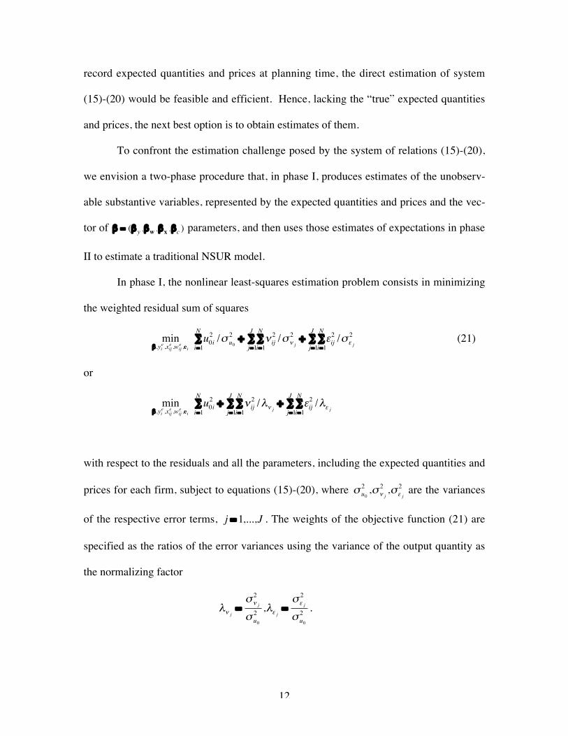
record expected quantities and prices at planning time, the direct estimation of system

(15)-(20) would be feasible and efficient. Hence, lacking the “true” expected quantities

and prices, the next best option is to obtain estimates of them.

To confront the estimation challenge posed by the system of relations (15)-(20),

we envision a two-phase procedure that, in phase I, produces estimates of the unobserv-

able substantive variables, represented by the expected quantities and prices and the vec-

tor of

€

β = (β y ,βw ,βx ,βc ) parameters, and then uses those estimates of expectations in phase

II to estimate a traditional NSUR model.

In phase I, the nonlinear least-squares estimation problem consists in minimizing

the weighted residual sum of squares

€

minβ,yi

e ,xije ,wij

e ,ei u0i

2 /σ u0

2

i=1

N∑ + ν ij

2 /σν j

2

i=1

N∑

j=1

J∑ + εij

2 /σε j

2

i=1

N∑

j=1

J∑ (21)

or

€

minβ,yi

e ,xije ,wij

e ,ei u0i

2

i=1

N∑ + ν ij

2 /λν ji=1

N∑

j=1

J∑ + εij

2 /λε ji=1

N∑

j=1

J∑

with respect to the residuals and all the parameters, including the expected quantities and

prices for each firm, subject to equations (15)-(20), where

€

σ u02 ,σν j

2 ,σε j

2 are the variances

of the respective error terms,

€

j =1,...,J . The weights of the objective function (21) are

specified as the ratios of the error variances using the variance of the output quantity as

the normalizing factor

€

λν j=σν j

2

σ u02 ,λε j =

σε j

2

σ u02 .

13

We assume that an optimal solution of the phase I problem exists and can be found using

a nonlinear optimization package such as, for example, GAMS (see Brooke et al. [1988]).

With the estimates of the expected quantities and prices obtained from phase I, a

traditional NSUR problem can be stated and estimated in phase II using conventional

econometric packages such as SHAZAM (Whistler et al. [2001]). For clarity, this phase

II estimation problem can be stated as

€

minβ,ei

′ e i ˆ Σ −1eii=1

N∑ (22)

subject to

€

yi = f e( ˆ x ie ,β y ) + u0i , (23)

€

wi = cye( ˆ y i

e , ˆ w ie ,βc )fxe( ˆ x ie ,βw ) + ν i , (24)

€

xi = he( ˆ y ie , ˆ w ie ,βx ) + εi , (25)

where

€

( ˆ y ie , ˆ w ie , ˆ x ie ) are the expected quantities and prices of the i-th firm estimated in

phase I and assume the role of instrumental variables in phase II. The matrix

€

ˆ Σ can be

updated iteratively to convergence. Given the complexity of the nonlinear EIV system of

equations specified above, the standard errors of the estimates will be computed by a

bootstrapping approach, as discussed in details further on.

The specification of the functional form of the production function constitutes a

further challenge toward the successful estimation of the above system of production and

cost functions. In the case of self-dual technologies such as the Cobb-Douglas and the

constant elasticity of substitution (CES) production functions, the corresponding cost

function has the same functional form and no special difficulty arises. For the general

case of more flexible functional forms, however, it is well known that the functional form

14

can be explicitly stated only for either the primal or the dual relations. The associated

dual functions exist only in an implicit, latent state. The suggestion, therefore, is to as-

sume an explicit flexible functional form for the cost function and to represent the associ-

ated implicit production function as a second-degree Taylor expansion. Alternatively,

one can use an appealing approach to estimation of latent functions presented by

McManus (1994) that fits a localized Cobb-Douglas function to each sample observation.

IV. An Application of the GAE Model of Production and Cost

The model and the estimation procedure described in section III have been applied to a

sample of 84 California cooperative cotton ginning firms. These cooperative firms must

process all the raw cotton delivered by the member farmers. Hence, the level of their out-

put is exogenous and their economic decisions are made according to a cost-minimizing

behavior. This is a working hypothesis that can be tested during the analysis.

There are three inputs: labor, energy and capital. Labor is defined as the annual

labor hours of all employees. The wage rate for each gin was computed by dividing the

labor bill by the quantity of labor. Energy expenditures include the annual bill for elec-

tricity, natural gas, and propane. British thermal unit (BTU) prices for each fuel were

computed from each gin’s utility rate schedules and then aggregated into a single BTU

price for each gin using BTU quantities as weights for each energy source. The variable

input energy was then computed by dividing energy expenditures by the aggregate energy

price.

A gin’s operation is a seasonal enterprise. The downtime is about nine months

per year. The long down time allows for yearly adjustments in the ginning equipment

15

and buildings. For this reason capital is treated as a variable input. Each component of

the capital stock was measured using the perpetual inventory method and straight-line

depreciation. The rental prices for buildings and ginning equipment was measured by the

Christensen and Jorgenson (1969) formula. Expenditures for each component of the

capital stock were computed as the product of each component of the capital stock and its

corresponding rental rate and aggregated into total capital expenditures. The composite

rental price for each gin was computed using an expenditure-weighted average of the

gin’s rental prices for buildings and equipment. The composite measure of the capital

service flow is computed by dividing total yearly capital expenditure by the composite

rental price.

Ginning cooperative firms receive the raw cotton from the field and their output

consists of cleaned and baled cotton lint and cottonseeds in fixed proportions. These out-

puts, in turn, are proportional to the raw cotton input. Total output for each gin was then

computed as a composite commodity by aggregating cotton lint and cottonseed using a

proportionality coefficient. For more information on the sample data see Sexton et al.

(1989).

We assume that the behavior of the ginning cooperatives of California can be ra-

tionalized with a Cobb-Douglas production function. Hence, the system of equations to

specify the production and cost environments is constituted of the following eight primal

and dual relations:

Cobb-Douglas production function

€

yi = A (xije )α j

j=1

3

∏ + u0i , (26)

16

Input price functions

€

wik = αk[A α jα j

i=1

3∏ ]−1/η(yi

e )1/η (wije )α j /η

j=1

3∏ /(xik

e )+ ν ik , (27)

Input derived demand functions

€

xij = α j[A αkαk

k=1

3

∏ ]−1/η(yie )1/η(wij

e )− ( αkk≠ j∑ ) /η

(wike )αk /η

k≠ j=1

3

∏ +εij , (28)

where

€

η =def

α jj∑ , j = 1,2,3, and

€

k = 1,2,3.

As discussed in previous sections, the consistent estimation of an errors-in-

variables model requires a priori knowledge of the ratio of the error variances. Since this

kind of information cannot be derived from the sample observations, we conducted a

Monte Carlo analysis of the model developed in section III in order to gauge the per-

formance of the primal-dual estimator under a misspecification of the ratio of the error

variances. Since the estimator is robust (as determined by the mean squared error statis-

tics reported in Table 1), we estimate the primal-dual model using the available sample

information and compute the standard errors of the estimates by a bootstrapping proce-

dure.

The system of Cobb-Douglas relations (26)-(28) was estimated by using the two-

phase procedure described in section III using the computer package GAMS (Brooke et

al. [1988]) for phase I and phase II. We must point out that with technologies (such as the

Cobb-Douglas production function) admitting an explicit analytical solution of the first-

order necessary conditions, either the input derived demand functions (28) or the input

price functions (27) are redundant in the phase I estimation problem, and thus either set

of equations can be eliminated as constraints. They are not redundant, however, in the

phase II NSUR estimation problem because, as noted earlier, all the primal and dual rela-

17

tions convey independent information in the form of their errors and the corresponding

probability distributions. Furthermore, neither the primal nor the dual relations would be

redundant in phase I if the specified technology were of the flexible form type.

The Monte Carlo analysis of the primal-dual estimator was performed with the

choice of the following “true” parameter values of the Cobb-Douglas specification: Effi-

ciency parameter

€

A = 0.81, production elasticities

€

αK = 0.43,αL = 0.48,αE = 0.27 , and

returns to scale

€

η =1.18. The input quantities were generated as

€

xij = xije + N(0,0.5),

where the latent expected quantities were taken as the original sample data. The input

prices were generated as

€

wij = wije + N(0,0.6) , where the latent expected prices were taken

as the original sample data. The choice of the normal error’s standard deviation was re-

lated to the scale of the corresponding latent variable and the desire to minimize negative

values of the associated observed variable. The output quantity was generated as

€

yi = A (xije )α j + N(0,1.5)j=1

3∏ . In each specification, the normal error has a zero mean and

€

σ standard deviation, and is signified by

€

N(0,σ ). Hence, for the input quantities, the true

variance is

€

σε j

2 = 0.25 while the true variance of the input prices is

€

σν j

2 = 0.36 ,

€

j = K ,L,E . Thus, the weights of the sum of squared residuals are

€

λεj = σε j

2 /σ u02 = 0.25 /(1.5)2 = 0.111 and

€

λνj = σν j

2 /σ u02 = 0.36 /2.25 = 0.16,

€

j = K ,L,E .

Three hundred samples were drawn for the Monte Carlo analysis, whose results are re-

ported in Table 1.

Table 1 is divided in three sub-tables relating to primal-dual, Mundlak and

McElroy’s models. The first three sections of Table 1 deal with the results of the primal-

dual estimator: In the first section, the lambda parameters were chosen with the true value

18

of the error variance ratios. Hence, the corresponding estimates are consistent and the

mean squared error statistics are relatively low, with the squared bias values also pretty

small. In the second section of Table 1 the lambda parameters’ (ratios of error variances)

values are three times as large as the true values. Yet, the mean squared error statistics

are of the same level as those for the true values of the lambda parameters. In particular,

the squared bias of the efficiency parameter

€

A is much lower than the corresponding sta-

tistic of the true model. In the third section of Table 1 the lambda parameters’ values are

between seven and ten times as large as the corresponding values of true model. Yet, this

gross mis-specification of the error variances induces only a relatively small (30 percent)

increase in the mean squared error statistics as compared to those of the true lambda ra-

tios.

In all the three cases, the mean values of the production elasticities are within a

remarkable narrow range of the true values and the corresponding standard deviations of

the estimates are small and stable. Therefore, the empirical evidence presented in Table 1

suggests that even a large mis-specification of the true values of the error variances in-

duces only a relatively small bias into the estimates.

The second section of Table 1 deals with Mundlak’s primal model. Given the

structure of the production and cost model presented in this paper, Mundlak’s primal

model comes in two versions. The first version assumes that there are no measurement

errors (the usual assumption) and the estimated model is similar to that exposed by

Mundlak (1996). The second version assumes an errors-in-variables specification with

€

ε ≡ 0 and the model to be estimated reduces to equations (12) and (13) in section II.

19

Table 1. Results of the Monte Carlo analysis: 300 samples

Primal-Dual. Trueλεj=.111, λνj=.16

286 SamplesMean Estimate

Standard De-viation

Estimate/Std Dev

MSE Squared Bias

A, efficiency 0.81 0.8341 0.1249 6.678 0.0161913 0.0005793 αΚ, capital 0.43 0.4207 0.0314 13.398 αL, labor 0.48 0.4829 0.0347 13.916 αE, energy 0.27 0.2773 0.0205 13.527 all inputs 0.0027564 0.0001485η, scale 1.18 1.1809 0.0850 13.893 0.0072246 0.0000008

Primal-DualMisspecifiedλεj=.333, λνj=.40


StandardDeviation

Estimate/Std Dev MSE

Squared Bias

A, efficiency 0.8070 0.1202 6.714 0.0144611 0.0000088αΚ, capital 0.4293 0.0319 13.457αL, labor 0.4928 0.0345 14.284αE, energy 0.2836 0.0206 13.767 all inputs 0.0029331 0.0003477η, scale 1.2056 0.0846 14.251 0.0078109 0.0006559

Primal-DualMisspecifiedλεj=1, λνj=1


StandardDeviation

Estimate/Std Dev MSE

Squared Bias


Mundlak PrimalTrue λνj=.16


StandardDeviation

Estimate/Std Dev MSE Squared Bias


Mundlak PrimalTrue λνj=.16


StandardDeviation



McElroy DualTrue λεj=.111


StandardDeviation


A, efficiency 0.5645 0.1034 5.459 0.0709756 0.0602833αΚ, capital 0.5265 0.0395 13.329αL, labor 0.6046 0.0444 13.617αE, energy 0.3528 0.0265 13.313 all inputs 0.1207709 0.1165337η, scale 1.4840 0.1072 0.1038848 0.0923922

20

The empirical results of the first version of the Mundlak model indicate very large

mean squared error statistics for all the parameters. The squared bias statistics are also

orders of magnitude larger than the corresponding biases of the primal-dual model. The

mean estimates of the parameters are very different from the true value and the corre-

sponding standard deviations are very large. The results of the second version of the

Mundlak model are considerably better but one must recall that nobody has ever esti-

mated such a primal model. Yet, the mean squared error statistics of this partial EIV

model are also orders of magnitude larger than any of the corresponding statistics of the

primal-dual model.

The third and final section of Table 1 reports the results of McElroy’s dual model

as specified in equations (9)-(11) of section II. In this model the assumption is that

€

y ≡ ye and w ≡ we and, thus the relevant system of equations to estimate are the derived

demand functions as expressed by equation (11). The empirical results reported in the

last section of Table 1 indicate that the mean estimates of the parameters are way off as

compared to the true values, the mean squared error statistics are much larger that the

corresponding statistics of the primal-dual model, as are the squared biases.

The summary conclusion of the Monte Carlo analysis performed in this paper

suggests that the primal-dual model is a robust estimator even under large mis-

specification of the error variances’ ratios. This result is a novel finding that has not been

previously reported in the econometric literature. When compared to either the primal

(Mundlak) or dual (McElroy) results, the estimates of the primal-dual model are consid-

erably closer to the true values of the parameters. On the strength of this finding we now

proceed to estimate the primal-dual model using exclusively the available sample infor-

21

mation and two specifications of the error variances’ ratios. The empirical results are re-

ported in Table 2.

Table 2. Estimates of the Primal-Dual Model of Production and Cost. Standard Devia-

tions computed by bootstrapping on 300 samples.

Primal-Dualλεj=.5, λνj=.5 Estimate

StandardDeviation

Estimate/Standard Deviation

A, efficiency 0.8284 0.0537 15.426 αΚ, capital 0.4098 0.0395 10.375 αL, labor 0.4796 0.0651 7.367 αE, energy 0.2696 0.0709 3.802η, scale 1.1590 0.0324 35.377

Primal-Dualλεj=1.0, λνj=1.0 Estimate

StandardDeviation

Estimate/Standard Deviation

A, efficiency 0.8087 0.0585 13.824αΚ, capital 0.4141 0.0417 9.930αL, labor 0.4862 0.0729 6.669αE, energy 0.2732 0.0782 3.494η, scale 1.1735 0.0353 33.244

The estimates and their bootstrap standard errors are not very different between

the two sets of estimates even though they depend on two different ratios of the error

variances. This result mimics the findings of the Monte Carlo analysis.

V. Conclusion

We tackled the 60-years old problem of how to obtain efficient estimates of a Cobb-

Douglas production function when the price-taking firms operate in a cost-minimizing

environment. The simplicity of the idea underlying the model presented in this paper can

be re-stated as follows. Entrepreneurs make their planning, optimizing decisions on the

22

basis of expected, non-stochastic information. When econometricians intervene and de-

sire to re-construct the environment that presumably led to the realized decisions, they

have to measure quantities and prices and, in so doing, commit measurement errors. This

background seems universal and hardly deniable. The challenge, then, of how to deal

with a nonlinear errors-in-variables specification was solved by a two-phase estimation

procedure. In phase I, the expected quantities and prices are estimated by a nonlinear

least-squares method. In phase II, this estimated information is used in a NSUR model to

obtain efficient estimates of the Cobb-Douglas technology. It is well known that consis-

tent estimates of an EIV model require the a priori knowledge of the ratio of the error

variances. A Monte Carlo analysis, however, has revealed that even a gross mis-

specification of these ratios is associated with estimates that are remarkably close to those

obtained under the choice of the true ratios.

In the process, the debate whether a primal or a dual approach is to be preferred

for estimating production and cost relations was put to rest by the demonstration that a

more efficient system is composed by both primal and dual relations that must be jointly

estimated. Only under special cases it is convenient to estimate either a primal (Mund-

lak’s) or a dual (McElroy’s) environment.

In connection with this either-primal-or-dual debate, it is often said (for example,

Mundlak 1996, p. 433): “In passing we note that the original problem of identifying the

production function as posed by Marschak and Andrews (1944) assumed no price varia-

tion across competitive firms. In that case, it is impossible to estimate the supply and

factor demand functions from cross-section data of firms and therefore (the dual estima-

tor)

€

ˆ γ p cannot be computed. Thus, a major claimed virtue of dual functions---that prices

23

are more exogenous than quantities--- cannot be attained. Therefore, for the dual esti-

mator to be operational, the sample should contain observations on agents operating in

different markets.”

After many years of pondering this non-symmetric problem, the solution is sim-

pler than expected and we can now refute Mundlak’s assertion. The key to the solution is

the assumption that individual entrepreneurs make their planning decisions on the basis

of their expectation processes, an assumption made also by Mundlak (1996, p. 431). The

individuality of such information overcomes the fact that econometricians measure a

price that seems to be the same across firms. In effect, we know that this uniformity of

prices reflects more the failure of our statistical reporting system rather than a true uni-

formity of prices faced by entrepreneurs in their individual planning processes. The

model proposed in this paper provides an operational dual estimator, as advocated by

Mundlak, by decomposing a price that is perceived as the same across observations into

an individual firm’s expected price and a measurement error.

The GAE model of production and cost presented here can be extended to a

profit-maximization environment and also to the consistent estimation of a system of

consumer demand functions.

24

References

Brooke, Anthony, Kendrick, David and Meeraus, Alexander. GAMS, A User’s Guide,

Boyd and Fraser Publishing Company. Danvers, MA, 1988.

Christensen, Lauritis R. and Jorgenson, Dale W. “The Measurement of U.S. Real Capital

Input 1929-1967.” Review of Income and Wealth, Series 15 (September 1969):

135-151.

Diewert, W. Erwin. “Application of Duality Theory.” In Frontiers of Quantitative

Economics, Contributions to Economic Analysis, Vol. 2, pp. 106-171, edited by

Intrilligator, Michael D. and Kendrick. David A. Amsterdam: North Holland,

1974.

Fuss, Melvyn and McFadden, Daniel, eds. Production Economics: A Dual Approach to

Theory and Applications, Amsterdam: North Holland, 1978.

Goldberg, Arthur S. “Maximum Likelihood Estimation of Regressions Containing

Unobservable Independent Variables.” International Economic Review

13 (February 1972):1-15.

Griliches, Zvi. “Errors in Variables and Other Unobservables” Econometrica

42 (November 1974):971-998.

Hoch, Irving. “Simultaneous Equation Bias in the Context of the Cobb-Douglas

Production Function.” Econometrica 26 (October 1958):566-578.

______. “Estimation of the Production Function Parameters Combining

Time-Series and Cross-Section Data.” Econometrica 30 (January 1962):4-53.

Klepper, Steven and Leamer , Edward E. “Consistent Sets of Estimates for Regression

With Errors in All Variables.” Econometrica 52 (January 1984):163-183.

25

Leamer, Edward E. “Errors in Variables in Linear Systems.” Econometrica 55

(July 1987):893-909.

Marschak, Jacob and Andrews, William H. Jr. “Random Simultaneous Equations and

the Theory of Production.” Econometrica 12 (January 1944):143-206.

McElroy, Marjorie B. “Additive General Error Models for Production, Cost, and

Derived Demand or Share Systems.” J. Political Economy 95

(August 1987):737-757.

McManus, Douglas A. “Making the Cobb-Douglas Functional Form an Efficient

Nonparameteric Estimation Through Localization.” Paper 94-31, Monetary and

Financial Studies. Board of Governors of the Federal Reserve. Washington D.C.,

September 1994.

Mundlak, Yair. “Estimation of the Production and Behavioral Functions from a

Combination of Cross-Section and Time-Series Data.” Pp. 138-166 in: Christ,

Carl F. et al., Measurement in Economics. Standford University Press, Stanford,

CA, 1963.

_________. “Production Function Estimation: Reviving the Primal.” Econometrica

64 (March 1996):431-438.

Nerlove, Marc. “Returns to Scale in Electricity Supply.” pp. 167-198, in Christ, Carl F. et

al., Measurement in Economics. Stanford, California, Stanford University Press,

1963.

Schmidt, Peter. “Estimation of a Fixed-Effect Cobb-Douglas System Using Panel Data.”

Journal of Econometrics. 37 (March 1988):361-380.

Sexton, Richard J., Wilson, Brooks M. and Wann, Joyce J. “Some Tests of the

26

Economic Theory of Cooperatives: Methodology and Application to Cotton Gin

ning.” Western Journal of Agricultural Economics 4 (July 1989):56-66.

Theil, Henry. Principles of Econometrics, John Wiley, New York, 1971

Whistler, Diana, White, Kenneth J., Wong, S. Donna and Bates, David. SHAZAM, The

Econometric Computer Program, User’s Reference Manual, Version 9.

Northwest Econometrics Ltd. Vancouver, B.C. Canada, 2001.

Zellner, Arnold, Kmenta, Jan and Dreze, Jacques. “Specification and Estimation of

Cobb-Douglas Production Function Models.” Econometrica,

34 (October 1966):784-795.

Zellner, Arnold. “Estimation of Regression Relationships Containing Unobservable

Independent Variables.” International Economic Review 11

(October 1970):441-454.

a primal-dual estimator of production and cost functions ... · a primal-dual estimator of...

Documents