a primal method for minimal cost flows with applications...

A Primal Method for Minimal Cost Flows with Applications to the Assignment andTransportation ProblemsAuthor(s): Morton KleinSource: Management Science, Vol. 14, No. 3, Theory Series (Nov., 1967), pp. 205-220Published by: INFORMSStable URL: http://www.jstor.org/stable/2628396 .Accessed: 13/10/2011 16:01

Your use of the JSTOR archive indicates your acceptance of the Terms & Conditions of Use, available at .http://www.jstor.org/page/info/about/policies/terms.jsp

JSTOR is a not-for-profit service that helps scholars, researchers, and students discover, use, and build upon a wide range ofcontent in a trusted digital archive. We use information technology and tools to increase productivity and facilitate new formsof scholarship. For more information about JSTOR, please contact [email protected].

INFORMS is collaborating with JSTOR to digitize, preserve and extend access to Management Science.

http://www.jstor.org

http://www.jstor.org/action/showPublisher?publisherCode=informs

http://www.jstor.org/stable/2628396?origin=JSTOR-pdf

http://www.jstor.org/page/info/about/policies/terms.jsp

MANAGEMENT SCIENCE Vol. 14, No. 3, November, 1967

Printed in U.S.A.

A PRIMAL METHOD FOR MINIMAL COST FLOWS WITH APPLICATIONS TO THE ASSIGNMENT AND

TRANSPORTATION PROBLEMS*t

MORTON KLEIN$

Columbia University

A simple procedure is given for solving minimal cost flow problems in which feasible flows are maintained throughout. It specializes to give primal algorithms for the assignment and transportation problems. Convex cost problems can also be handled.

1. Introduction

Suppose we have a network with vertices V = { 1, * , n}, directed edges E =

{ (i, j) - V X V}, a non-negative integral valued function k giving the maximum allowable flow ki1 over every edge, and a non-negative cost function a giving the cost aij associated with a unit of flow over any edge. A flow X of value v is an integral valued function defined on E satisfying

(1.1) < xij kii I (ij j) eE.

(1.2) V=I (zi - - i - 1,

= 0, i= 2,**,n-1,

- -=n.

Vertices 1 and n are, respectively, called the flow source and sink. The minimal cost flow problem is to find, among all flows X of value v, one

which minimizes

(1.3) Q(X) == J(i j)ZE xii aij .

The main computational procedures developed to date for solving this problem are the primal-dual type algorithms of Ford and Fulkerson [7], Busacker and Gowen (described in [3]), and Jewell [12]. These are dual methods in which feasible flows (those satisfying (1.1) and (1.2)) become available when the computations terminate. A similar method for convex cost flow problems has been given by Hu [9]. Fulkerson's "Out-of-Kilter" algorithm (described in [7]) is essentially a primal method in that it can be started with a feasible flow or one becomes available at an early stage. Another primal approach for problems with convex costs has also been suggested recently by Menon [14].

The assignment and transportation problems can be thought of as special minimal cost flow problems in the sense that their networks have a particular

* Received September 1966, revised April 1967, and accepted May 1967. t This research is supported by the Army, Navy, Air Force, and N.A.S. under a contract

administered by the Office of Naval Research; Contract Nonr 266(55). Reproduction in whole or in part is permitted for any purpose of the United States Government.

j The author is indebted to T. C. Hu and M. Florian for helpful suggestions.

205

206 MORTON KLEIN

bipartite form. Kuhn's "Hungarian Method" [13], a primal-dual type algorithm, and two variants: ([15] and one given in [7]) provide the most popular methods for solving these problems. Other methods are described by Flood [5] and Hoff- man and Markowitz [8]. Primal methods are also available: Dantzig's adaptation of the simplex method (described in [4]), the methods given by Beale [2], Flood [6], and, most recently, by Balinski and Gomory [1].

The purpose of this paper is to suggest that one more primal method can be added to the above arsenal for both minimal cost flow and assignment-transportation problems. With slight modification it can also be used for problems involving convex costs. It shares, with other primal methods, the property that it can be started with a "good" solution and a better one is always available in case early termination of computations is required.

2. A Minimal Cost Flow Algorithm

In this section we give a procedure for solving the minimal cost flow problem. We assume a familiarity with the maximal flow and shortest route problems together with the Ford-Fulkerson [7] methods for solving them.

The method suggested here is to first find a flow satisfying (1.1) and (1.2) by, say, the Ford and Fulkerson maximum flow routine [7] (pp. 17-18). Given such a flow X, we then construct an associated network G(X) which has the same vertices as the original network and directed edges, as follows:

(2.1) E(X): (ij ), if xij < kij and xji - 0,

(j, i), if Xii > 0, with revised capacities:

(2.2) k': kij = kij - xij, if xi; < kij and xji = 0,

ji = xii, if x) > 0, and with revised edge costs:

/ / (2.3) a': ad = aij, if xii < kij and xji = 0,

aji = -aij, if Xij > O.

These revised edge costs are simply those associated with increasing or cancelling the flow by one unit on these edges: The revised capacities indicate the extent to which this can be done.

Now, we use a result proved in Busacker and Saaty ([3], pp. 256-257). Theorem. X is a minimal cost flow if and only if there is no directed cycle C in

G(X) such that the sum of the costs around C's edges are negative. (A directed cycle is a sequence of distinct directed edges of the form { (io, i1) (il, i2) **

(ip, jq) (iq, io) } involving distinct vertices.) An immediate consequence of this theorem is that a test of the optimality of

the flow X is at hand if G(X) can be checked for the existence of a negative cost directed cycle. Further, if such a cycle is found an improved flow is obtained by sending a positive unit flow around this cycle. Such a flow alteration obviously leads to a lower total cost and also leaves the flow value v unchanged.

A PRIMAL METHOD FOR MINIMAL COST FLOWS 207

Fortunately, there are known methods for locating negative cost directed cycles. The Fulkerson "Out-of-Kilter" procedure [7] (pp. 162-169) is one. Various shortest route algorithms may also be used; of these, we shall use a "Matrix Multiplication" procedure due to Murchland [16) (as described by Hu [10]) which is designed to find the shortest routes between every pair of vertices in a network. Although this method (in common with other shortest route algorithms) requires the assumption of non-negative directed cycle costs; it also may be used to locate such a cycle.

We need only put the above observations together to obtain an

Algorithm for Minimal Cost Flows

1. Use the Ford-Fulkerson maximal flow routine (or any other) to find a flow X of value v.

2. Form the associated network G(X) according to (2.1), (2.2), and (2.3). 3. Test for the existence of a negative directed cycle C in G(X) using the

matrix multiplication method described in [10] as follows: a) Form an n X n matrix D(X) in which each row and column is associated

with a vertex of G(X), with entries dij = alj as given by (2.3), andwithall other entries equal to infinity.

b) Pivot Steps: For each value k = 1, 2, * , n, in turn, perform the replacement operation,

(2.4) dij = min (dij, dik + dkj)

for all i, j 7 k. c) Repeat b) until some entry drr becomes negative (indicating the existence of

a negative cost cycle involving vertex r) or until the replacement operation has been completed for k = n with all dii > 0. If the latter occurs, it indicates that G(X) does not contain a negative cycle and that the flow being tested is optimal.

d) If a negative cost directed cycle C is found to involve vertex r, we shall call r the initial point. We now suggest that it is computationally convenient to use the Ford-Fulkerson shortest route index reduction method to trace the edges of C by using it to find the shortest route from the initial point to every other vertex in G(X). (Step 4, below) (It is possible to keep track of the edges which give rise to the negative cycle in the matrix multiplication method as indicated by Hu in [11]. However, "keeping track" is cumbersome and requires the storage of much unneeded data. The index reduction routine appears to be more economical for this purpose.)

4. The negative cycle tracing routine is as follows: a) Let r be the initial point. Assign it the label (-, 7r(r) = 0). Assign all other

vertices labels of the form (-, -r(i) = co). b) Search for an edge (j, k) such that

7r(j) + dJk ? r(k)

and then either change the label on vertex k to (j, 7r(j) + djk), if the inequality is strict (case a) or, change the label to ({k, j}, 7r(k)) if equality holds (case b). Continue until the initial point receives a label of the form (i*, 7r(r) < 0).

208 MORTON KLEIN

c) The negative cycle C can now be found by tracing backwards from r to i* * , to r. If vertices are encountered with more than one label (case b in (b)), then sub-cycles of cost zero will be encountered; these are discarded. For example, if tracing yields a sequence of the form (r, i1) (il , i2) (i2 , i1) where vertex ii had the double label, say, ({i2, i3}, d), the sub-cycle (il, i2) (i2, i1) has associated cost zero. The tracing process is then continued from vertex i3. Since there may be more than one negative cycle, one can, in tracing, encounter a negative cycle which does not involve the initial point. In this case, this cycle can be used as a basis for the improved flow.

5. Given C, an improved flow X' is given by

xij =xij 7 if (i, i) 'VC,

(2.5) = xij - 3, if (j, j) e C and ale < 0, - xj + 3, if (i, j) e C and ad > 0,

where a = min ij)ec {k'j}, i.e., a is the largest amount of flow which can be sent around C.

Return to Step 2. Example. Suppose a minimal cost flow of value 4 is to be imposed on the follow-

ing network from vertex 1 to vertex 5. Costs and capacities are indicated according to the legend { cost, capacity} on each edge.

We start with an arbitrary flow X of value 4, indicated in Figure 2 (omitting Step 1 for a problem of this size).

Step 2. G(X) is then as shown in Fig. 3, where negative cost edges are indicated by dashed lines.

Step 3. The matrix multiplication routine starts with D(X) as given below. 1 2 3 4 5

1 00 4 1 00 00

2 X 00 00 00 1

3 - 1 2 00 3 00

4 00 00 -3 00 00

5 00 0o0 o -2 00

It ends (at pivot step k = 4) when d55 = -2, 1 2 3 4 5

1 0 3 -1 -4 4

2 oo oo oo oo 1

3 - 1 -2 0 3 3

4 -4 -1 -2 0 0

5 -6 -3 -4 pi-2 -2

Hence, vertex 5 is the initial point for the cycle tracing routine.


Source 9 fSink

\11,8} {2, 5} {2 X 4}

FIGURE 1

\ 0

3 4

FIGURE 2

?4{1,2i 51

{-1 4}\I 3%,_ {3,6}

{-3, 4}

FIGURE 3

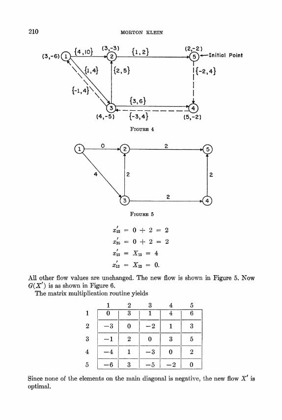
Step 4. After application of the cycle tracing routine G(X) has vertex labels as indicated in Figure 4. C is found bytracingback from vertex 5 to 2, from 2 to 3, from 3 to 4, and from 4 to 5. That is, C = {(5, 4) (4, 3) (3, 2) (2, 5)}.

Step 5.

a = min {ks4, k 3, k12, k15}

= min {4, 4, 5, 2 } = 2

and the new flow X' is

4= 4 - 2 = 2

=34 4 - 2 = 2

210 MORTON KLEIN

{4 ,IQ} (3 'I3) {1, 2} (-2) - --Initial Point

{1 14} {2, 5} l{24

3lk_

4}\ ~ 3

3_ {3X6}= _ g

(4.-5 ) {-3, 4} (X2

FIGURE 4

FIGURE 5

X32= 0 + 2 - 2

X25= 0 + 2 = 2

X13 X13 = 4

X12 - X12 = 0.

All other flow values are unchanged. The new flow is shown in Figure 5. Now G(X') is as shown in Figure 6.

The matrix multiplication routine yields

1 2 3 4 5 1 0 3 14 6

2 -3 0 -2 1 3

3 -1 2 0 3 5

4 -4 1 -3 0 2

5 -6 3 -5 -2 0

Since none of the elements on the main diagonal is negative, the new flow X' is optimal.


1 2\{-3,2}

FIGURE 6

Men Jobs

{4,IO} 5a i

\?' } {-26,4}I {21 {2 2}

1 4

{-3, 2}

sou J ensJob

{0,\ I/ d <0,1

FIG. 7. Network representation of an assignment problem

3. Application to the Assignment Problem

In this section we show how the method described above specializes for solving the assignment problem.

The assignment problem is to fill n jobs by as many men at least total cost. If aij represents the cost of using man i in job j, then a mathematical statement of the problem is to find a permutation matrix X = (xi1) of order n, which minimizes the total cost Q(X) = E xijaij, where xij = 1 implies that man i (i = 1,... , n) is assigned to job j (j = n + 1, .. ., 2n).

The equivalent minimum cost flow problem (following Ford and Fulkerson) is illustrated for the case v = n = 3 in Figure 7.

212 MORTON KLEIN

Algorithm for Assignment Problem

1. The algorithm can be started with any feasible (trial) solution. (This cor- responds to finding a flow of value v = n.) It is frequently advantageous to try to choose a "good" solution using some heuristic rule, e.g. the "Least-Cost Rule" given by Dantzig in [4] (p. 309).

Let X be a trial solution and A'(X) an associated matrix with elements

(3.1) a = -aii, if xij > 0,

- aij, if Xii = O.

where i = 1,* * *, n and j = n + 1, ***,2n. Further, let D(X) be the (2n) X (2n) matrix with rows and columns each

corresponding to both the men and the jobs of the problem and with elements.

(3.2) diq = co, i, j = 1, .., n or i, j = n + 1, ** , 2n,

= ai, =1,***,n, j = n + 1, ***,2n,

= -aji, xji > i = n + 1, ***,2n; j = 1, **,n

= 00 X Oji = " " cc

2. Test for the existence of a negative cycle as in step 3 of the algorithm for minimal cost flows using D as described in (3.2) above as the cost matrix.

If all dii > 0, the algorithm terminates and the trial solution is optimal. Other- wise, let drr be the first negative element encountered and use r as the initial point for the cycle tracing routine next.

3. Because of the special bipartite form of the network interpretation of the problem (the source and sink can be dropped since their associated edges have zero costs) it is convenient to do the cycle tracing routine using the matrix A'(X). This is done by means of a series of alternate row and column labelings on A' with each successive row (column) label giving the cost associated with following a traceable route from the initial point to the column (row) from which the current cost is measured.

Let (Mi, di) be a label assigned to column j of A'. Then the implication is that there is a directed route from the initial point to Mi and a directed edge to (job) column j such that the total cost is di . The row labels (Jj, dj) are defined similarly.

A convenient notational device is to write ax; if aj' < 0 and xi; > 0. Let Jr be the initial point.' Label column r (-, 0). 1. Label each row (Jr ar I )a 2. Label each columnj # r, (Mi, di + a-).

1 If a row vertex Mr is the indicated initial point, the labeling routine can be followed as written by interchanging the rows and columns of A'.


3. Label each row ({ Jk}, m1nj (dj + I a )j 1)) where each Jk represents a column at which the minimum is attained.

4. Label each column (Mi, di + a-d). 5. Continue steps 3 and 4 until the initial point's label becomes negative. The negative cost cycle, C, can be identified by tracing back from the initial

point according to the succession of adjacent row and column labels until the initial point is encountered for the second time or some other vertex is encountered twice indicating a negative cycle not involving the initial point. Then, an improved trial solution X' is given by

(3.3) ;= xiJ, if (Mow Jj) q C,

= 0, if Mi, Jj e C and xij = 1,

= 1, if lM, Jj I C and xij = 0,

where the notation I M., Jj I indicates that either (Mi, Jj) or (J,? Mi) is an element of C.

Return to step 2. Example. Suppose (using a least-cost rule) the first trial solution is x7 =

X25= X38 X46 = 1, then A'(X) and D(X) are given below.

Ji J6 J7 J8 M1 2 3 -1 1

M2 -5 8 3 2 A'(X)

M3 4 9 5 -1

M4 8 -7 8 4

M1 M2 M3 M4 J5 J6 J7 J8 _ _ _ _ - _ _ _ _ _ _ _ 2 3 1

112 5 8 3 2

M3 4 9 5 1

M4 8 7 8 4 D (X) =_- _ -

J6 -5

J7 ~ ~ ~ ~ -

J7 -

(Note: All unmarked entries have values di =

The matrix multiplication routine (step 2), at pivot step k = 5, gives

214 MORTON KLEIN

M1 M2 M3 M4 J6 J6 J7 J8

Ml -3 2 3 0 -1

2 ~ ~ 05 8 3 2

J3 -1 4 7 2 1

314 3 8 7 6 4

J6 -5 0 3 -2 -3

J6 -4 -7 1 0 -1 -2

J7 -1 -4 1 2 -@ -2

_____ -1 ___ __ 4 7 2 1

Since d77 < 0, J7 is the initial point for the cycle tracing routine. The appropriate labels on A'(X) are shown below.

>Initial point

JL J6 J7 Js

ml 2* 3 -1 * - J7,I J5

M2 5* 8 3* 2 J7, 3 1 2 J7I 3

M3 4 9 5 -1 2,1Li,2

M4 8 -7 8 4 J7,_8 1 i, 6 M2, -2 1 4,11 - 0 1 M3,4 4 ? l ! M~~~1l, -1 !

tStop

The elements of C are (J7, M1), (Ml, J5), (J5, M2), (M2, J7); these are indicated by asterisks (*) above. The new trial solution is, from (3.2) x' = x2 =

xI6 = S38 = 1. Its total cost is 13. The example is continued. D(X') is

m_ _ l2 M3 M4 J5 J6 J7 J8 M3 =_2 3 11

312 5 8 3 2

M3 4 9 5 1

314 8 7 8 4

J5 -2

J6 -7

J7 -3

J o _ _ _ - 1 _ _ _ _ _ _ _ _ _ _ _


and the matrix multiplication routine yields

M1 M2 M3 M4 J6 J6 J7 J8 l 0 -2 -1 -4 3 3 1 0

M2 3 0 1 -1 5 -6 4 2

M3 2 0 0 -2 4 5 3 2

M4 5 3 3 0 7 8 6 4

Jo -2 -4 -3 -6 0 1 -1 -2

J6 -2 -4 -4 -7 0 0 -1 -3

J7 0 -3 -2 -4 2 3 0 - 1

J8 1 -1I - 1 -3 3 4 2 0

Since all elements on the main diagonal are non-negative, X' is an optimal solution.

4. An Algorithm for the Transportation Problem

The method given here for the transportation problem is, with slight alteration, the sameQ.as that suggested for the assignment problem. The reason for this computational similarity is, of course, the well-known relationship between the two problems: each is a special case of the other.

We suppose that the transportation problem involves shipments of a single commodity from n plants P1, * * *, Pn I with capacities cl, * * *, c, to m warehouses Wol, . * *, Wn+m with requirements r7n+l 2 * * * . If acj represents the cost of shipping a unit from Pi to Wj, and xij the quantity shipped from Pi to Wj, the problem is to minimize the total cost

(4.1) Q(X) Eij= Z j1 Z x-1ai

constrained by

(4.2) EZ=i xij = rj , i=n+ n + in;

Zi=n+f xij = ci, i = 1, ,n;

xij = 0 1, ... .

where we assume that the ci's and r/'s are positive integers, and E ci = E r1. We omit the network formulation of the problem and go directly to the com-

putational procedure. The terminology is the same as that used for the assignment problem except that we speak of plants and warehouses instead of men and jobs.

1. Trial Solutions: Although the computational procedure can be written so that one can work with any trial solution satisfying (4.2), it is convenient to restrict ourselves to the "basic feasible solutions", possibly degenerate, which

216 MORTON KLEIN

are used in Dantzig's adaptation of the simplex method for transportation problems. These solutions contain, at most, m + n - 1 positive entries. They also have the property that no cycles can be formed by their positive entries. These two properties may also be justified by simple combinatorial arguments [6].

Suppose X is a trial solution (i.e., it satisfies (4.2) and the above). We again define the associated matrix A'(X) by

(4.3) atj = -ai1, if xij > O, - aj, if xij = 0,

and write acj if a'ij < 0 and xii > 0. Let D(X) be the (m + n) X (m + n) matrix with elements

(4.4) dij= oo, ij= 1, ,n or ij=n+1,**,n+ m

= aij , i = 1, ... n; j = n + 1, ** n + m

=-aji , xji > l 0+ ,in m

= x xji = I i

2. Matrix Multiplication Routine: Terminating with an initial point corresponding to first negative main diagonal element, or, if no such element is negative, with the conclusion that the trial solution is optimal.

3. Cycle Tracing Routine: Using the matrix A'(X); suppose Wr is the initial point.2 Label its column (-, 0).

1. Label each row (W7, j aI) 2. Label each column j # r ({Pk}, mini{di + a7Q4) where each Pk is a row

at which the minimum is attained. 3. Label each row ({Wk}, minj{dj + I a1j I 1) 4. Label each column (I{Pk}, mini{di + at} ) 5. Continue steps 3 and 4 until the initial point's label becomes negative. The negative cost cycle is then obtained by tracing backwards from the

initial point, discarding any zero cost sub-cycles which may be encountered. As indicated earlier, a negative cycle, not involving the initial point, may be discovered before a return to the initial point. This may be used to find an improved solution.

Let X(C) be the entries of X whose subscripts correspond to those of C, i.e., if I Pi, Wj I e C then xij e X(C), and index these entries (with superscripts) as follows: assign the index 1 to any entry whose value is zero. (There is at least one such entry by virtue of our use of "basic feasible" trial solutions.) Now, following the cycle (in either direction) continue with successive positive integers: 2, 3, * , k until all elements in X(C) have been indexed. Note that the index k is an even number.

2 If a row vertex P7 is the initial point, the labeling routine can be followed with the rows and columns of A' interchanged.


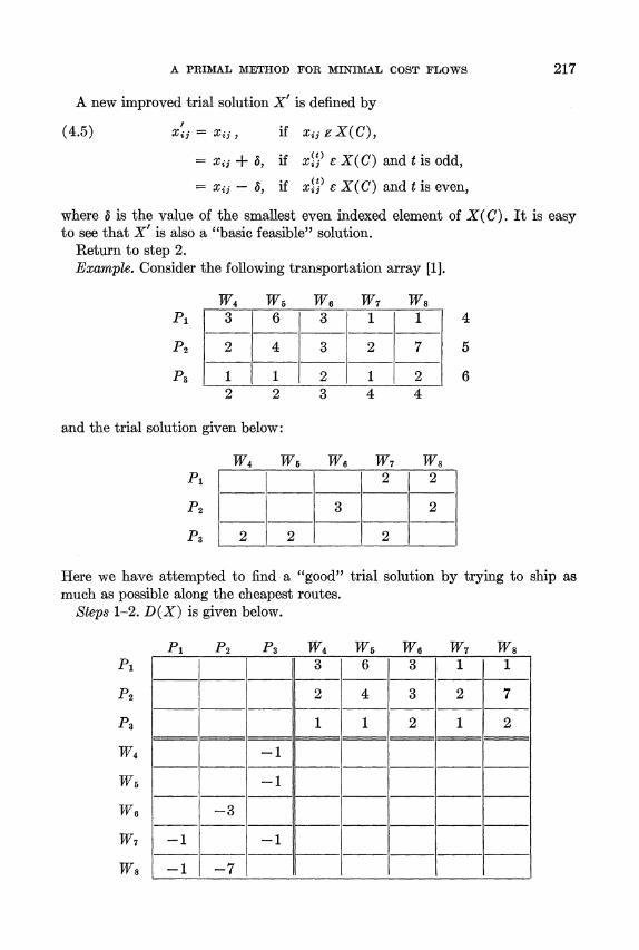
A new improved trial solution X' is defined by

(4.5) x.j x/ , if xije X(C),

xij + 5, if x~t ? X(C) and t is odd,

xij - , if X( ) ? X(C) and t is even,

where a is the value of the smallest even indexed element of X(C). It is easy to see that X' is also a "basic feasible" solution.

Return to step 2. Example. Consider the following transportation array [1].

W4 W5 W6 W7 W8 P1 3 6 3 1 1 4

P2 2 4 3 2 7 5

P3 1 1 2 1 2 6 2 2 3 4 4

and the trial solution given below:

W4 W6 w6 W7 W8

Pi 2 2

P2 3 2

Ps 2 2 2

Here we have attempted to find a "good" trial solution by trying to ship as much as possible along the cheapest routes.

Steps 1-2. D(X) is given below.

P1 P2 P3 W4 W6 W6 W7 W8

Pi 3 -6 3 1 -1

P2 2 4 3 2 7

P3 1 1 2 1 2

W4 -1

146 -1

W6 -3

w7 -1 -

W 8 - 1 - 7 _ _ _ _ _ _ _ _ _ _ _ _ _

218 MORTON KLEIN

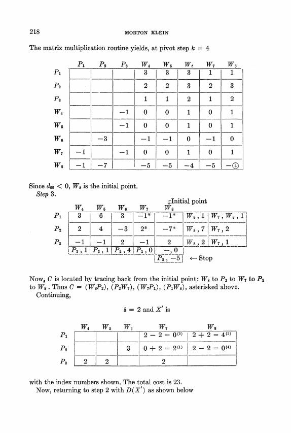
The matrix multiplication routine yields, at pivot step k = 4

P1 P2 P3 W4 W5 WI6 W7 Ws P1i 3 -3 -3 -1 -1

P2 2 2 3 2 3

P3 1 1 2 1 2

W4 -1 0 0 1 0 1

W5 -1 0 0 1 0 1

W6 -3 -1 -1 0 -1 0

W7 -1 -1 0 0 1 0 1

W8 - 1 -7 -5 -5 -4 -5 -?G)

Since dca < 0, Ws is the initial point. Step 3.

,-Initial point W4 W5 W6 W7 W8

P1 3 6 3 -1* --1* -W8, 1'W7, W8l

------------- P2 2 4 1-3 2* -7t* Ws 2 7 1 W7 2 2

P3 - 1 - 1 2 - 1 2 7W8,2'W7, 1

P3,1 IP3, 1 P2, 4P1, I -,o 1 IP2, -5' <- Stop

Now, C is located by tracing back from the initial point: W8 to P2 to W7 to PI to WBs. Thus C = (TWSP2), (P2W7), (TW7P1), (P1VW8), asterisked above.

Continuing,

a = 2 and X' is

TV4 WT W6 W7 W8

P1 2 - 2 = 0(2) 2 + 2 = 40)

P2 3 0 + 2 2(1) 2 - 2 = 0(4)

P3 2 2 2

with the index numbers shown. The total cost is 23. Now, returning to step 2 with D(X') as shown below


P1 P2 P3 TV4 WV W6 W7 W8

P - 6 3 1 1

P2 2 4 3 2 7

P3 1 2 1 2

W4 -1

WT5 -1

W6 -3

W7 -2 -1

the matrix multiplication routine gives us

Pi P2 P3 TV4 TV TV6 TV7 TWs P1 0 -1 013 2 1 2

P2 2 0 1 2 4 3 3 3

P3 1 -1 0 1 3 2 2 2

TV4 0 -2 -1 0 2 1 1 1

W5 0 -2 -1 0 0 1 1 1

TV6 -1 -3 -2 -1 1 0 0 0

TV. 0 -2 -1 0 2 1 0 1

TV8 -1 -2 -1 0 2 1 0 0

Since no main diagonal elements are negative, the trial solution X' is optimal.

5. Convex Cost Flows

As indicated by Hu [9], the primal-dual type algorithms for minimal (linear) cost flow problems can be adapted to handle cases in which the edge cost func- tions are piece-wise linear convex. The basic notion, used here also, is to use the (changing) marginal costs associated with possible unit flow alterations in the associated graph. In our case, this means that cyclical flow changes will involve only one unit of flow (i.e., 6 = 1) and the edge costs for the associated graph will depend somewhat more on the current flow values on each edge than they did in the linear cost problem.

If we represent each edge cost function by bij, the problem is to find the minimum of

220 MORTON KLEIN

(5.1) Q(X) = Z(i,j),E bij(xij)

constrained by (1.1) and (1.2). All we need to do is to note that the network G(X) associated with a feasible

flow X, is defined as before, except that the revised (marginal) edge costs blj are given by

b= [bij(xij + 1) - bij(xij)], if xij < kij and xji = 0;

and

=bi = - - bij(xij-1)], if xxj > 0.

This, plus our previous observation that 5 = 1, enables the use of the minimal cost flow routine. Similar alterations can be made to handle the transportation problem with convex costs.

References

1. BALINSKI, M. L. AND GOMORY, R. E., "A Primal Method for the Assignment and Trans- portation Problems," Management Science, Vol. 10, No. 3, 1964, pp. 578-593.

2. BEALE, E. M. L., "An Algorithm for Solving the Transportation Problem When the Shipping Cost Over Each Route is Convex", Naval Research Logistics Quarterly, Vol. 6, No. 1, 1959, pp. 43-56.

3. BUSACKER, R. G. AND SAATY, T. L., Finite Graphs and Networks, McGraw-Hill, New York, N.Y., 1965.

4. DANTZIG, G. B., Linear Programming and Extensions, Princeton University Press, Princeton, N.J., 1963.

5. FLOOD, M. M., "An Alternative Proof of a Theorem of Konig as an Algorithm for the Hitchcock Distribution Problem", in Combinatorial Analysis, American Mathe- matical Society, Providence, Rhode Island (1960) pp. 299-307.

6. -, "On the Hitchcock Distribution Problem", Pacific Journal of Mathematics, Vol. 3, No. 2 (1953) pp. 369-386.

7. FORD, L. R., JR. AND FULKERSON, D. R., Flows in Networks, Princeton University Press, Princeton, N.J., 1962.

8. HOFFMAN, A. J. AND MARKOWITZ, H. M., "A Note on Shortest Path, Assignment, and Transportation Problems", Naval Research Logistics Quarterly, Vol. 10, No. 4 (1963) pp. 375-379.

9. Hu, T. C., "Minimum Convex-Cost Flows in Networks", Naval Research Logistics Quarterly, Vol. 13, No. 1 (1966).

10. - , "A Decomposition Algorithm for Shortest Paths in a Network", IBM Research Center Report, RC 1562, Feb. 1966.

11. -', "Revised Matrix Algorithm for Shortest Paths", IBM Research Center Report, RC 1478, Sept. 1965.

12. JEWELL, W. S., "Optimal Flow Through Networks With Gains", Operations Research, Vol. 10, No. 4 (1962) pp. 476-499.

13. KUHN, H. W., "The Hungarian Method for the Assignment Problem", Naval Research Logistics Quarterly, Vol. 2, Nos. 1 and 2 (1955) pp. 83-97.

14. MENON, V. V., "The Minimum Cost Flow Problem With Convex Costs", Naval Re- search Logistics Quarterly, Vol. 12, No. 2 (1965) pp. 163-172.

15. MUNKRES, J., "Algorithms for the Assignment and Transportation Problems", Journal of the Society for Industrial and Applied Mathematics, Vol. 5, No. 1 (1957) pp. 32-38.

16. MURCHLAND, J. D., "A New Method for Finding All Elementary Paths in a Complete Directed Graph", LSE-TNT-22, London School of Economics, Oct. 1965.

a primal method for minimal cost flows with applications...

Documents