a primer in statistics, study design, and epidemiology · a primer in statistics, study design, and...
TRANSCRIPT

Evidence-Based Medicine Journal Club
A Primer in Statistics, Study Design, and
Epidemiology
August, 2013

Rationale for EBM • Conscientious, explicit, and judicious use
– Beyond clinical experience and physiologic principles
– Scientific and mathematical rigor • Current best evidence
– Hierarchy of evidence • Making decisions about patients
– Clinical actions and consequences – Impact of treatment or usefulness of test

Steps in Practice of EBM
• Ask appropriate question • Determine what information is required
to answer question • Conduct literature search • Select best studies • Critically assess evidence for validity
and utility • Extract message and apply to clinical
problem

The real goal
• Assess the relationship between an exposure/treatment and an outcome/disease
• Look at a sample; apply it to the population

Searching for Evidence
• Medical database – PubMed
www.pubmed.gov – Ovid – Web of Knowledge – Cochrane database – NOT GOOGLE
• Up-to-Date—nice overview, but not a systematic evaluation

Critical Assessment 3 Essential Questions
1. What are the results?
2. Are the results of the study valid? 3. Will the results help me in caring
for my patients?

What does valid mean?
• The extent to which the associations found in the study sample reflect the true associations in the population – Internal validity—inferences drawn about
the population that provided the subjects – External validity—extent generalizable to
different populations and circumstances

Assessing Validity
1. Why was the study done and what was the hypothesis?
2. What type of study was done?
3. Was the design appropriate to answer the question posed?

Study Types
• Observational vs. Experimental – Descriptive
• Case report/series
– Analytical • RCT/N-RCT • Cohort • Case-Control • Cross-Sectional • Ecological

Other Types
• Systematic Reviews – Meta-analysis
• Expert reviews – Practice Guidelines
• Cost-effectiveness analyses

From Shulz and Grimes, Handbook of Essential Concepts in Clinical Research, 2006

Hierarchy of Evidence
1. Systematic Reviews and Meta-analysis of RCTs*
2. Randomized Controlled Trials 3. N-RCT / Cohort Studies 4. Case-Control Studies 5. Cross-Sectional surveys 6. Case Reports

Levels of Evidence
• Level I – Randomized controlled trials (RCT)
• Level II-1 – Controlled trials without randomization (N-RCT)
• Level II-2 – Cohort – Case-Control
• Level II-3 – Cross-sectional studies – Uncontrolled investigational studies
• Level III – Descriptive studies – Expert opinion

Translating Evidence to Recommendations
• Based on quality and quantity of evidence
– A: Good evidence to support the recommendation
– B: Fair evidence to support the recommendation
– C: Insufficient evidence to support the recommendation
– D: Fair evidence against the recommendation
– E: Good evidence against the recommendation

Hill’s Criteria for Causation
• Temporal sequence • Strength of association • Dose response/biological gradient • Consistency of association • Biologic plausibility • Coherence with existing knowledge • Experimental evidence • Analogy • Specificity of association

Bias
• Systematic Error leading to over- or under-estimation of the true relationship or parameter as exists in the population of interest: – Design – Conduct – Analysis

Types of Bias
1. Selection – Incomparability in ways groups of
subjects are chosen – Volunteer bias
2. Information/Misclassification – Incomparability in quantity and quality
of information gathered or in way managed • Look for disease/exposure more
thoroughly in one group • Recall bias
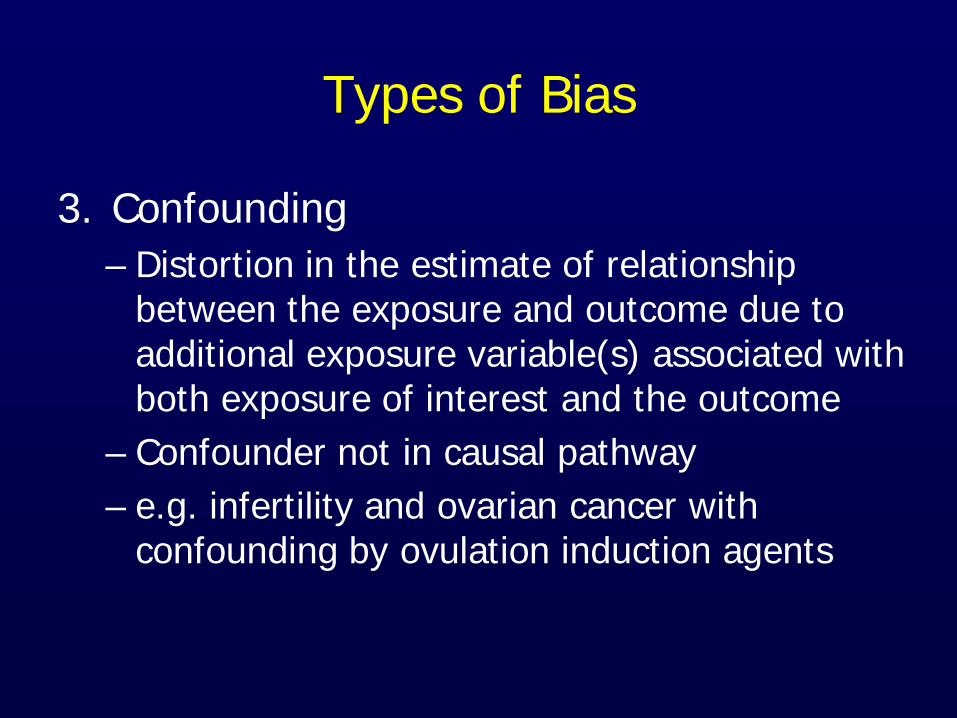
Types of Bias
3. Confounding – Distortion in the estimate of relationship
between the exposure and outcome due to additional exposure variable(s) associated with both exposure of interest and the outcome
– Confounder not in causal pathway – e.g. infertility and ovarian cancer with
confounding by ovulation induction agents

Controlling Confounding
A. Adjust in analysis phase but have to: – Know what they are and measure
1. Stratification by exposure 2. Regression: multiple confounders
B. Limit in design phase: 3. Restriction: exclude potential confounder 4. Matching: ensure groups similar for
potential confounder 5. Randomization: Known and unknown
factors

Descriptive studies
• Case Report/Series – Show how people develop a condition
over time and describe the characteristics
• No comparison group • No assessment of association • E.g. cases of TTP/HUS, unusual
histology, etc.

Analytical Studies

Ecological Study
• Examines population level association of disease frequency and exposure
• Uses group as unit of analysis – e.g. % skilled birth attendance and
maternal mortality • No individual level risk • Generate hypotheses

Cross Sectional Study/Survey
• Assess exposure and disease status at a single point in time for each patient – e.g. Alcohol use and
infertility • No temporal
relationship evaluated

Cross-Sectional Study
• Strengths – Efficient – No waiting for outcome
• Weaknesses – No causal relationship – Impractical for rare disease

Case Control Study
• Identifies subjects based on presence or absence of disease/outcome
• Go backward in time to assess exposures
Do cases have a stronger history of exposure than controls?

Case Control Study
• Benefits – Good for rare disease – Cheaper – Efficient
• Limitations
– Bias • Selection • Recall
– Incidence cannot be determined • Size of the source population is unknown
– Temporal relationship may be unclear

Case Control Study Risk estimation
Odds Ratio – Odds of exposure history in cases/odds of
exposure history in controls • A/C ÷ B/D = AD/BC
Cases Controls
Exposed A B
Unexposed C D

What does an odds ratio of 3 mean?
• Literally – A history of exposure is 3 times more
likely to be found in cases compared to controls
• Clinical Application – The disease is 3 times more common
among the exposed than unexposed

Cohort Study
• Identify patients by presence or absence of an exposure and follow-up over a period of time – Prospective – Retrospective – Ambidirectional
Does outcome develop more commonly in the exposed than unexposed?

Cohort/Follow-up Study
• At time=0 – Exposure status: known – Disease status: negative
• Follow to some point in future • During course of study:
– Get disease – Die – Lost to f/u – Leave at risk pool

• Benefits – Define Incidence – Good for rare exposure and common disease – Temporal relationship – Dose response
• Limitations – Not as good for rare disease – Long follow-up – Cost – Selection bias in selection of unexposed – Observer bias – Retrospective cohort only possible if detailed
records available
Cohort/Follow-up Study

Relative Risk
• Proportion of exposed group who develop outcome/proportion of unexposed group who develops outcome
Disease No Disease
Exposed A B Unexposed C D
RR= A/A+B ÷ C/C+D

Measures of Disease Frequency • Incidence
– Occurrence of NEW cases of disease in an at risk population of interest over a stated period of time:
– Incidence rate: new cases per # at risk for given time—cases/person years
– RATE must include TIME • Cumulative Incidence
– What proportion of at risk patients developed the outcome in the given period of time
– Used to predict probability or RISK

• Prevalence – Proportion of individuals with disease
in a population at risk at a single time point
• ** In general: risk, ratio or rate
Measures of Disease Frequency

Design Advantages Disadvantages
Cohort •Establish sequence of events •Can study several outcomes •Number of events increases with time •Yields Incidence, Relative Risk •With prospective, control subject selection and measurements •Good for rare exposure
•Large sample size •Long duration •Problematic for rare disease
Cross-Sectional •Study several outcomes •Short duration •Yields Prevalence
•Sequence of events not determined •Problematic for rare predictors or outcomes •Does not yield incidence or true relative risk
Case-Control •Useful for rare conditions •Efficient •Yields Odds ratio
•Potential bias, confounding •Sequence of events not determined •Limited to one outcome •Potential survivor bias •Does not yield incidence or true risk

Clinical Trials
• Assigned exposure prior to occurrence of outcome
• Randomization is only way to minimize bias and confounding
• Blinding minimizes subject and observer bias

Randomization
• Each subject has same independent chance of being allocated to any of the treatment groups
• Goal is to balance known and unknown confounders between groups

Basic Concepts in Clinical Statistics

What does statistical analysis allow us to do?
•Take findings from the sample and infer the truth in the population •Provides a point estimate of the unknowable population parameter
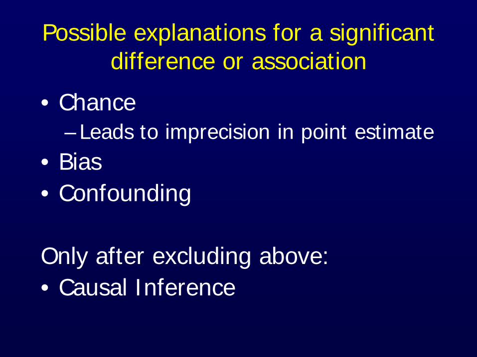
Possible explanations for a significant difference or association
• Chance – Leads to imprecision in point estimate
• Bias • Confounding
Only after excluding above: • Causal Inference

What is α?
• How much you are willing to let go to chance
• Probability of rejecting the null hypothesis in favor of the alternative hypothesis when there is no true difference
• Type I error • Arbitrary 0.05

What is β?
• Probability of failing to reject the null hypothesis, when in fact it is false and a true difference actually exists
• Type II error • Often set at 0.2 or 0.1

Power
• Probability of detecting as statistically significant a hypothesized point estimate of difference given a study size
• Power=1 - β

What affects Power?
• Sample Size of the study • Magnitude of difference/effect size • α level of significance • Rate of outcome in the unexposed • Type of measurement
– Continuous vs. dichotomous outcome

Study Size Determination
• Based on: – Magnitude of effect you want to be
able to detect – Baseline outcome incidence in
controls (or exposure incidence) – Power – α – Selection ratio of cases and controls

What does p mean?
• Probability, if the null hypothesis is true, if you repeated the experiment you would find results as or more extreme than those obtained
• A non-significant p does not mean there is no association
• Says nothing about bias and confounding
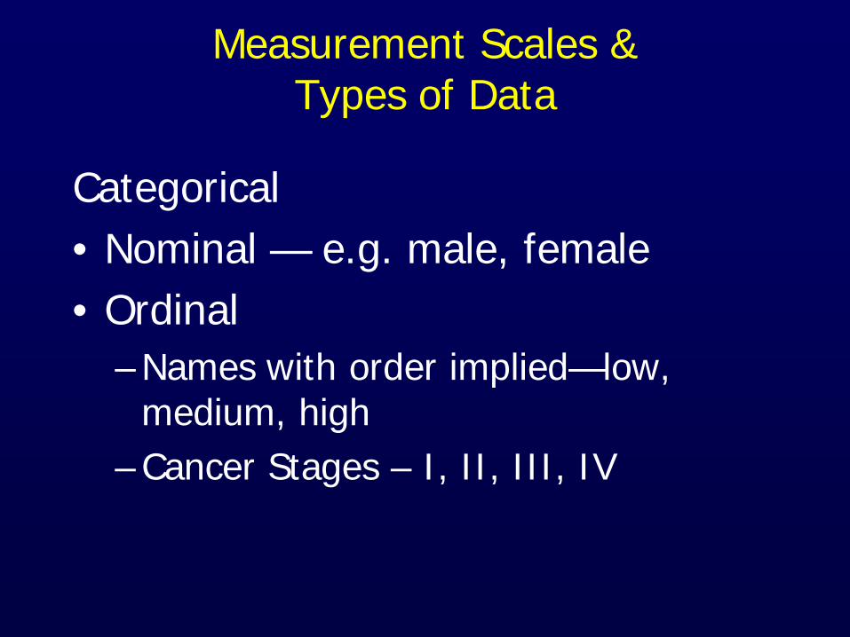
Measurement Scales & Types of Data
Categorical • Nominal — e.g. male, female • Ordinal
– Names with order implied—low, medium, high
– Cancer Stages – I, II, III, IV

Measurement Scales & Types of Data
Numeric • Discrete/Interval
– Finite number of intervals--# of pregnancies
• Continuous—e.g. BP, weight

Distribution of data and types of statistical tests
• Normal distribution – Affects types of statistical
tests that can be used • Parametric tests
– Certain assumptions made about the data based on normal distribution
• Non-parametric – Looks at rank order and
ignores absolute differences
– No assumptions about distribution
– Useful for small studies

Comparison of “average” measurement between 2 groups
• t-test – Comparison of Means – Normal distribution
• Mann-Whitney U/Wilcoxon Rank Sum – Comparison of Medians – Used for non-normal data or ordinal
scale data

• Allows for before and after • Paired t-test
– Parametric test
• Wilcoxon matched-pairs – Non-parametric
Comparison of “average” measurement in same group twice

Compare means or medians between 3 or more groups
• One Way ANOVA (F-test) – Means
• Kruskal-Wallis ANOVA – Medians

Test for proportions to compare distribution of variables or outcomes
• Compare gender between exposed and unexposed; outcome (Y/N) by exposure
• Chi-square analysis – If small sample size, need to use
Fisher’s exact test

Correlation • Strength and direction of
straight line association between two continuous variables – Height/weight; age/cholesterol
• Pearson’s correlation coefficient (r) – Parametric
• Spearman’s rank correlation coefficient (ρ) – Non-parametric
• Each correlation coefficient has a p value to show likelihood of arising by chance
Positive correlation
Inverse correlation

Regression
• Numerical relation between 2 or more quantitative variables allowing one (the dependent variable) to be predicted from the others – Predict weight from age, race, gender, and
height – Predict likelihood of PTB from race, parity,
weight • Statistically it is also a way to adjust for
confounders that can have an effect on the outcome of interest

Comparison Parametric Test Non-parametric Test
Means t-test Mann-Whitney U (medians)
Repeated observations in same individual/group
Paired t-test Wilcoxon matched pairs
Means in 3 or more groups
ANOVA Kruskall-Wallis ANOVA
Difference in proportions
--
Chi-square; Fisher’s exact
Strength of Association between continuous variables
Pearson’s correlation coefficient (r)
Spearman’s Correlation coefficient (ρ)
Relationship between variables
Linear regression; multiple regression
--

Measures of Association/Effect
• How do groups differ with respect to an outcome/disease – Relative—think division – Absolute—think subtraction

What’s the difference between A and B? How are the effects of the intervention or
exposure expressed?
• How much better or worse does the exposure make the patient – Relative risk/Odds ratio – Absolute risk – Number needed to treat

Association and impact
• Relative risk – The amount by which risk is
reduced/increased by exposure compared to control
• Absolute risk reduction – Absolute amount by which risk is changed
by exposure
• Number needed to treat – How many patients need to be exposed to
prevent one adverse outcome

Example Relative Risk reduction= 10/100÷30/100= 0.33 Absolute Risk reduction= .3 - .1 = .2 Number needed to treat= 1/Absolute risk reduction NNT= 5
Sx Return
Sx Free
Lupron 10 90
Surgery 30 70
Endometriosis patients 12 months after intervention

Odds ratio vs. Relative Risk?
• Odds ratio – Odds in favor of
exposure among cases to odds in favor of exposure among non-cases
• Relative risk – Proportion of
exposed with disease to proportion of unexposed with disease
Exposed Unexposed Disease A B
No disease C D
OR= A/B ÷ C/D = AD/BC
RR= A/A+C ÷ B/B+D=
A(B+D) ÷ B(A+C)
•With rare disease, OR and RR are similar because A and B are small.
•If disease prevalence >10-15%, OR overestimate magnitude of effect.

Accuracy
• Measurement of the variable is what you intend to assess
• What percent of all tests have given the correct result
• Bias – Observer – Subject – Instrument

Precision
• Repeated measurement with minimal variation – Observer – Instrument – Subject
• Reproducibility

Accuracy and Precision

Confidence Intervals
• Estimates strength of the evidence • Provides measure of precision of
findings • Range in which expect values to fall
95% of the time if trial repeated an infinite number of times
• Real meaning: 95% chance that the real result lies within the range of these values

Confidence Intervals What do they mean?
• Narrow CI – More precise – More definitive study – Because only 1 in 40 chance that true
result > and 1 in 40 that true result < limits
– Larger studies---narrower CI • If CI does not cross null value, then
findings significant
Parameters related to clinical and diagnostic tests

Test properties • Sensitivity
– Proportion of people with target disorder in whom test is positive
– Ability of test to detect disease when present
• Specificity – Proportion of people without disorder in
whom result is negative – Ability of test to detect absence of disease
when not present • Tell you about test in general
– NOT INFLUENCED BY DISEASE PREVALENCE
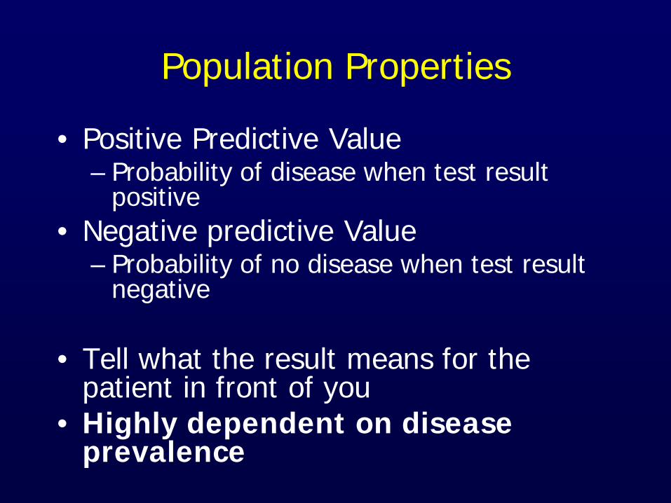
Population Properties
• Positive Predictive Value – Probability of disease when test result
positive • Negative predictive Value
– Probability of no disease when test result negative
• Tell what the result means for the
patient in front of you • Highly dependent on disease
prevalence

Disease present
Disease absent
Test + A B
Test - C D
Sensitivity= a/a+c
Specificity= d/b+d
PPV= a/a+b
NPV= d/c+d
Accuracy= a+d/a+b+c+d A & D = Concordant cells B & C = Discordant cells