A PRIMER ON DATA MASKING TECHNIQUES FOR NUMERICAL DATA

Krish Muralidhar

Gatton College of Business & Economics

My Co-author

I would first like to acknowledge that most of my work in this area is with my co-author Dr. Rathindra Sarathy at Oklahoma State University

Introduction

Data masking deals with techniques that can be used in situations where data sets consisting of sensitive (confidential) information are “masked”. The masked data retains its usefulness without compromising privacy and/or confidentiality. The masked data can be analyzed, shared, or disseminated without risk of disclosure.

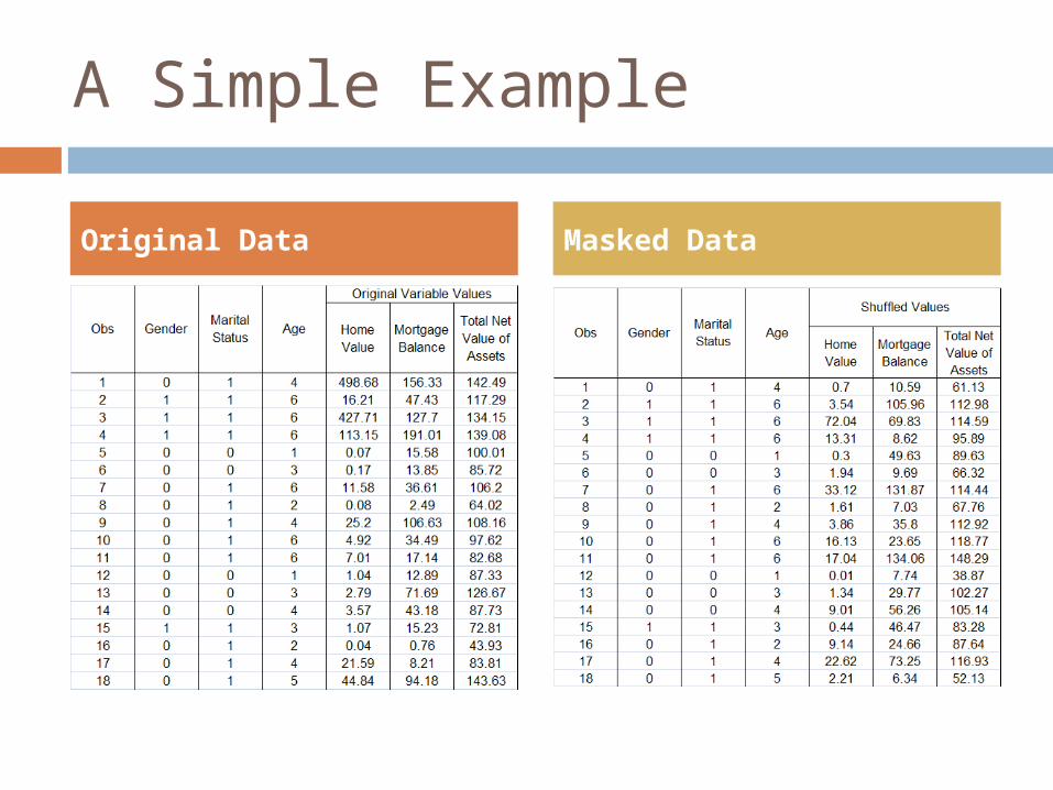
A Simple Example

Original Data Masked Data

Objectives of Data Masking

Minimize risk of disclosure resulting from providing access to the data

Maximize the analytical usefulness of the data

What this talk is not about … We are talking about protecting data that is

made available to users, shared with others, or disseminated to the general public

We are not dealing with unauthorized access to the data

Encryption is not a solution We cannot perform analysis on encrypted data

There are a few exceptions To perform analysis on the data, it must be

decrypted Decrypted data offers no protection

What this talk is not about … Since we have the data set, we know the

characteristics of the data set. We are trying to create a new data set that essentially contains the same characteristics as the original data set. We are not trying discern the characteristics of the original data set using the information in the masked data. In other words, I will not be talking about Agrawal and Srikant Or about the “distributed data” situation

In addition, since most of you are probably familiar with the CS literature on this area, I will focus on the literature in the “statistical disclosure limitation” area

Purpose of Dissemination

It is assumed that the data will be used primarily for analysis at the aggregate level using statistical or other analytical techniques The data will not be accurate at the

individual record level

Aggregate versus Micro Data The organization that owns the data could

potentially release aggregate information about the characteristics of the data set

The users can still perform some types of analyses using the aggregate data, but limits the ability of the users to perform ad hoc analysis

Releasing the microdata provides the users with the flexibility to perform any type of analysis

In this talk, we assume that the intent is to release microdata

Other Protection Measures

Restricted access Query restrictions Other methods

The Data

Typically, the data is historical and consists of Categorical variables (or attributes) Numerical variables

Discrete variables Continuous variables

In cases where identity is not to be revealed, key identification variables will be removed from the data set (de-identified)

De-identification does not necessarily prevent Re-identification

The common misconception is that, in order to prevent disclosure, all that is required is to remove “key identifiers”. However, even if the “key identifiers” are removed, in many cases it would be easy to indentify an individual using external data sources Latanya Sweeney’s work on k-anonymity The availability of numerical data makes it

easy to re-identify records through record linkage

Data Masking

Since de-identification alone does not prevent disclosure, it is necessary to “mask” the original data so that an intruder, even using external sources of data, cannot Identify a particular released record as

belonging to a particular individual Estimate the value of a confidential

variable for a particular record accurately

Who is an intruder?

Every user is potentially an intruder

Since microdata is released, we cannot prevent the user from performing any type of analysis on the released data

Must account for disclosure risk from any and all types of analyses Worst case scenario

The focus of our research

Data masking techniques are used to mask all types of data (categorical, discrete numerical, and continuous numerical)

The focus of our research, and of this talk, is data masking for continuous numerical data

The Data Release Process

Identify the data set to be released and the sensitive variables in the data

Release all aggregate information regarding the data Characteristics of individual variables Relationship measures Any other relevant information

Release non-sensitive data Since my focus is on numerical microdata, I will assume

that all categorical and discrete data are either released unmasked or are masked prior to release

Release masked numerical microdata

Characteristics of a good masking technique

Minimize disclosure risk (or maximize security)

Minimize information loss (or maximize data utility)

Other characteristics Must be easy to use

The user must be able to analyze the masked data exactly as he/she would the original data

Must be easy to implement

Disclosure Risk

Dalenius defines disclosure as having occurred if, using the released data, an intruder is able to identify an individual or estimate the value of a confidential variable with a greater level of accuracy than was possible prior to such data release

Minimum Disclosure Risk

A data masking technique minimizes disclosure risk, IFF, the release of the masked microdata does not allow an intruder to gain additional information about an individual record over and above what was already available (from the release of aggregate information, the non-confidential variables, and the masked categorical variables) Does not mean that the disclosure risk from the entire

data release process is minimum; only that the disclosure risk from releasing microdata is minimized

Can be achieved in practice

Practical Measure of Disclosure Risk Identity Disclosure

Re-identification rate Value disclosure

Variability in the confidential attribute explained by the masked data

Minimum Information Loss

Information loss is minimized IFF, for any arbitrary analysis (or query), the response from the masked data is exactly the same as that from the original data

Impossible to achieve in practice Since an arbitrary analysis may involve a

single record, the only way to achieve this objective is to release unmasked data

Information Loss … continued In practice, we attempt to minimize information

loss by maintaining the characteristics of the masked data to be the same as that of the original data

From a statistical perspective, we attempt to maintain the masked data to be “similar to” the original data so that responses to analyses using the masked data will be the approximately same as that using the original data Maintain the distribution of the masked data to be

the same as the original data

Some Practical Measures of Information Loss

Ability to maintain The marginal distribution Relationships between variables

Linear Monotonic Non-monotonic

Simple Masking Approaches

Noise addition Micro-aggregation Data swapping Other similar approaches

Any approach in which the masked value yij (the masked value for the jth variable of the ith record) is generated as a function of xi.

An Illustrative Example

A data set consisting of 2 categorical variables, 1 discrete, and 3 (confidential) numerical variables

50000 records

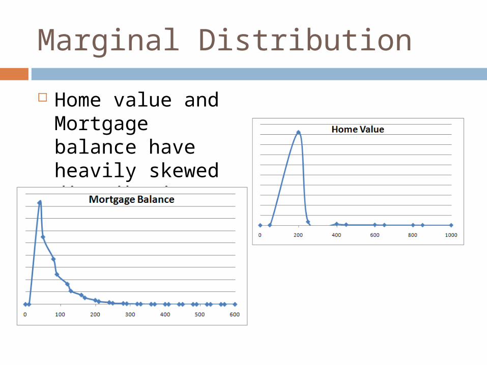
Marginal Distribution

Home value and Mortgage balance have heavily skewed distributions

Relationships

Relationships are not necessarily linear Measured by

both product moment and rank order correlation

Relationship Measures

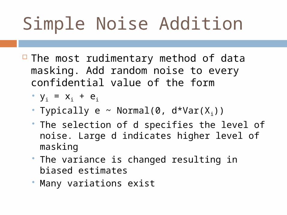
Simple Noise Addition

The most rudimentary method of data masking. Add random noise to every confidential value of the form yi = xi + ei

Typically e ~ Normal(0, d*Var(Xi)) The selection of d specifies the level of noise.

Large d indicates higher level of masking The variance is changed resulting in biased

estimates Many variations exist

Problems with Noise Addition The addition of noise results in an

increase in variance This can be addressed easily, but there

are other issues that cannot be, such as The marginal distribution is modified All Relationships are attenuated

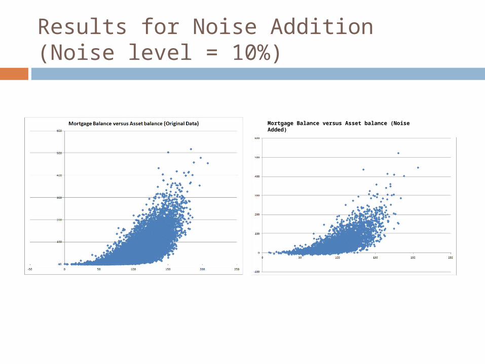
Results for Noise Addition(Noise level = 10%)

Mortgage Balance versus Asset balance (Noise Added)

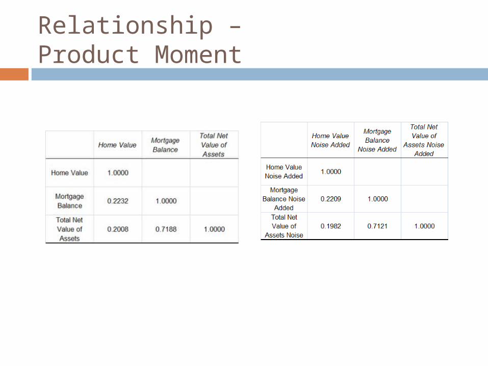
Relationship – Product Moment

Looks good …

Everything looks good Bias is small Relationships seem to be maintained

So what is the problem? The problem is security Since very little noise is added, there is

very little protection afforded to the records

High Disclosure Risk

The correlation between the original and masked values is of the order of 0.99. The masked values themselves are excellent predictors of the original value. Little or no “masking” is involved.

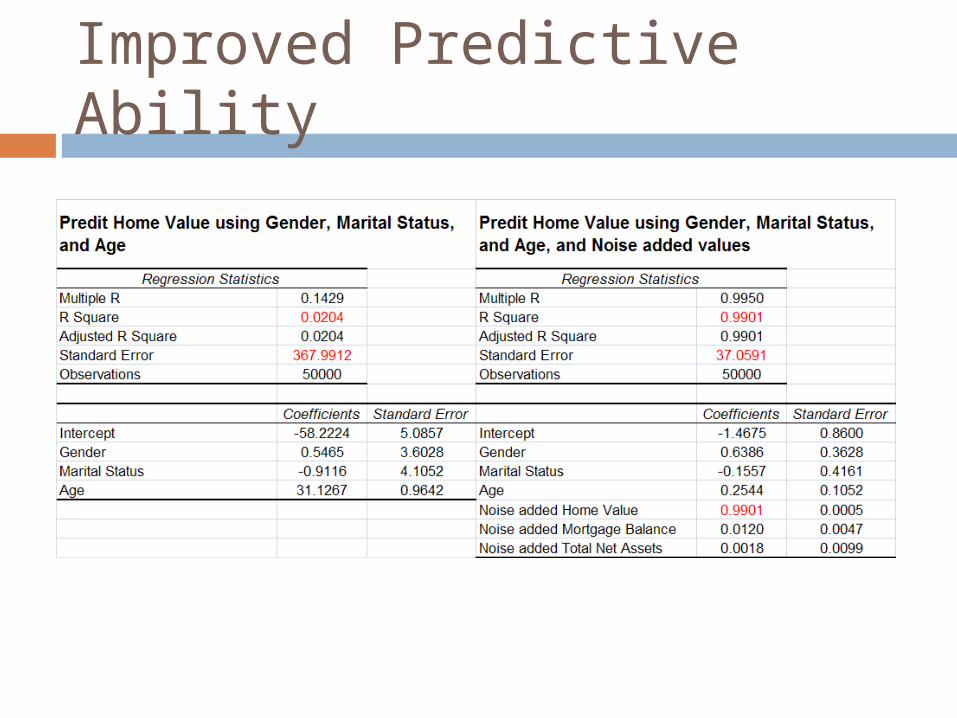
Improved Predictive Ability

Disclosure Risk versus Information Loss

Adding very little noise (10% of the variance of the individual variable) results in low information loss, but also results in high disclosure risk

In order to decrease disclosure risk, it would be necessary to increase the noise (say 50% of the variance), but that would result in higher information loss

Results for Noise Addition(Noise level = 50%)

At first glance, it does not seem too bad, but on closer observation, we notice that there are lots of negative values that did not exist in the original data Negative values

can be addressed

Mortgage Balance versus Asset balance (Noise Added)

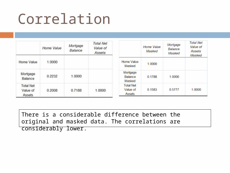
Correlation

There is a considerable difference between the original and masked data. The correlations are considerably lower.

Marginal Distribution of Home Value

The marginal distribution is completely modified

This is an unavoidable consequence of any noise “addition” procedure

Summary

In summary, noise addition is a rudimentary procedure that is easy to implement and easy to explain. There is always a trade-off between disclosure risk and information loss. If the disclosure risk is low (high) then the corresponding information loss is high (low).

Unfortunately, this is an inherent characteristic of all noise based methods of the form Y = f(X,e) whether the noise is additive or multiplicative or some other form

Sufficiency based Noise Addition

Recently, we have developed a new technique that is similar to noise addition, but maintains the mean vector and covariance matrix of the masked data to be the same as the original data Offers the same characteristics as noise

addition, but assures that results for traditional statistical analyses using the masked data will be the same as the original data

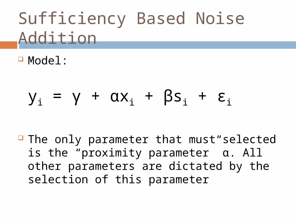
Sufficiency Based Noise Addition Model:

yi = γ + αxi + βsi + εi

The only parameter that must selected is the “proximity parameter” α. All other parameters are dictated by the selection of this parameter

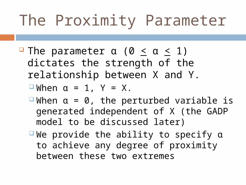
The Proximity Parameter

The parameter α (0 < α < 1) dictates the strength of the relationship between X and Y. When α = 1, Y = X. When α = 0, the perturbed variable is

generated independent of X (the GADP model to be discussed later)

We provide the ability to specify α to achieve any degree of proximity between these two extremes

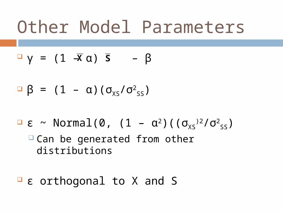
Other Model Parameters

γ = (1 – α) – β

β = (1 – α)(σXS/σ2SS)

ε ~ Normal(0, (1 – α2)((σXS)2/σ2

SS) Can be generated from other distributions

ε orthogonal to X and S

X S

Note that …

In order to maintain sufficient statistics, it is NECESSARY that the model for generating the perturbed values MUST be specified in this manner

Disclosure Risk

There is a direct correspondence between the proximity parameter α and the level of noise added in the simple noise addition approach. This procedure will result in incremental disclosure risk except when α = 0

The level of noise added is approximately equal to (1 – α2)

Information Loss

Information loss characteristics of the sufficiency based approach is exactly the same as that of the simple noise addition approach with one major difference. Results of statistical analyses for which the mean vector and covariance matrix are sufficient statistics will be exactly the same using the masked data as they are using the original data.

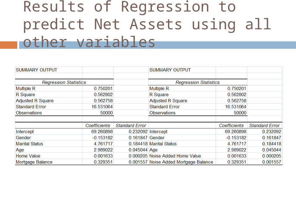
Results of Regression to predict Net Assets using all other variables

Simple versus Sufficiency Based Noise Addition If noise addition will be used to mask the

data, we should always use sufficiency based noise addition (and never simple noise addition). It provides all the same characteristics of simple noise addition with one major advantage that, for many traditional statistical analyses, it provides the guarantee that the masked data will yield the same results as the original data.

Microaggregation

Replace the values of the variables for a set of k records in close proximity with the average value of k records Many different methods of determining close proximity

Univariate microaggregation where each variable is aggregated individually

Multivariate microaggregation where the values of all the confidential variables for a given set of records are aggregated

Results in variance reduction and attenuation of covariance All relationships are modified … some correlations higher others

are lower Poor security even for relatively large k Consistent with the idea of “k anonymity” since at least k

records in the data set will have the same values

Univariate MA (k = 5) ExampleGood information loss characteristics but poor disclosure risk characteristics

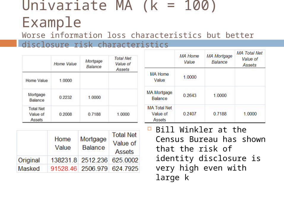
Univariate MA (k = 100) ExampleWorse information loss characteristics but better disclosure risk characteristics

Bill Winkler at the Census Bureau has shown that the risk of identity disclosure is very high even with large k

Rank Based Data Swapping

Swap values of variables within a specified proximity When the swapped

values are in close proximity, it results in low information loss but high disclosure risk and vice versa

The proximity is usually specified by the rank of the record

The advantage of data swapping is that it does not change (or perturb) the values; the original values are used The marginal distribution

of the masked data is exactly the same as the original

Unfortunately, it results in high information loss and offers poor disclosure risk characteristics

Data Swapping (Rank Proximity = 0.2% or the closest 100 records)

Information loss is low Unfortunately disclosure

risk is very high The correlation between

original and masked net asset value is 0.999

Data Swapping (Rank Proximity = 10% or the closest 5000 records)

Now information loss is very high, but disclosure risk is better

The problem with these approaches

There is an inherent problem with all approaches that generate the perturbed value as a function of the original value …. Y ~ f(X,e) These include all noise addition approaches, data swapping,

microaggregation, and any variation of these approaches

Using Delanius’ definition of disclosure risk, all these techniques result in disclosure

If we attempt to improve disclosure risk, it will adversely affect information loss (and vice versa)

What we need …

Is a method that will ensure that the released of the masked data does not result in any additional disclosure, but provides characteristics for the masked data that closely resemble the original data

From a statistical perspective, at least theoretically, there is a relatively easy solution

Conditional Distribution Approach

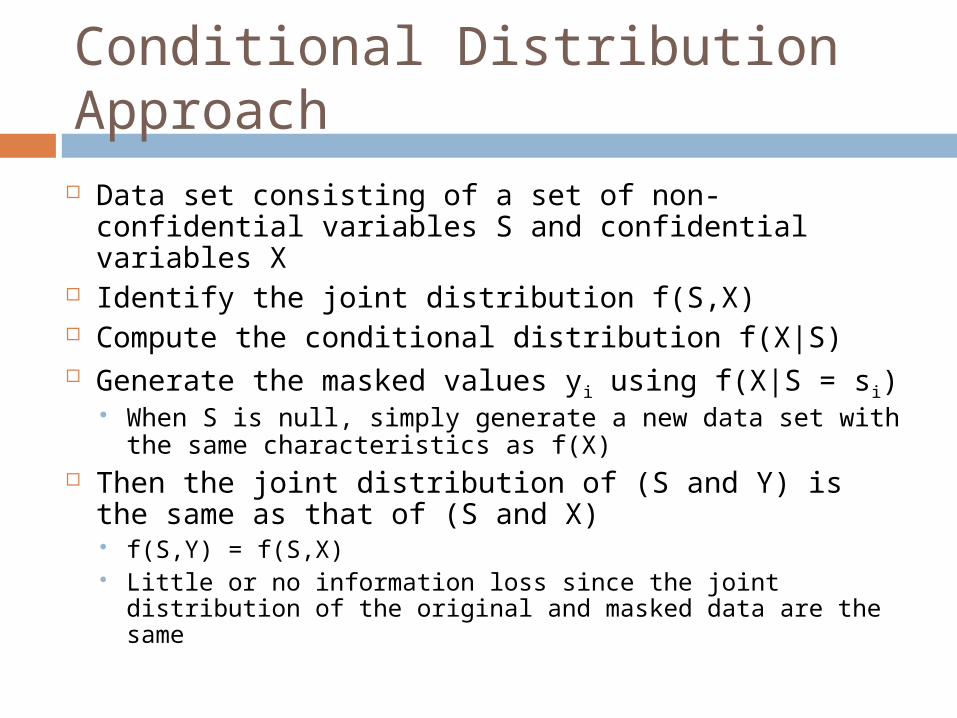
Data set consisting of a set of non-confidential variables S and confidential variables X

Identify the joint distribution f(S,X) Compute the conditional distribution f(X|S) Generate the masked values yi using f(X|S = si)

When S is null, simply generate a new data set with the same characteristics as f(X)

Then the joint distribution of (S and Y) is the same as that of (S and X) f(S,Y) = f(S,X) Little or no information loss since the joint distribution of

the original and masked data are the same

Disclosure Risk of CDA

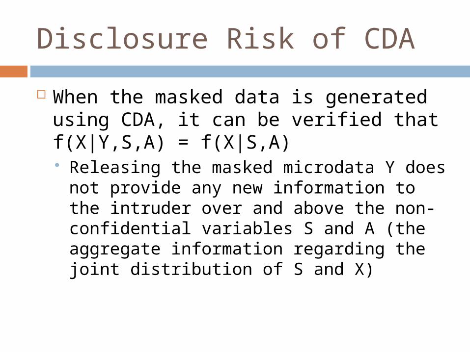
When the masked data is generated using CDA, it can be verified that f(X|Y,S,A) = f(X|S,A) Releasing the masked microdata Y does not

provide any new information to the intruder over and above the non-confidential variables S and A (the aggregate information regarding the joint distribution of S and X)

CDA is the answer … but

The CDA approach results in very low information loss and minimizes disclosure risk and represents a complete solution to the data masking problem

Unfortunately, in practice Identifying f(S,X) may be very difficult Deriving f(X|S) may be very difficult Generating yi using f(X|S) may be very difficult

In practice, it is unlikely that we can use the conditional distribution approach

Model Based Approaches

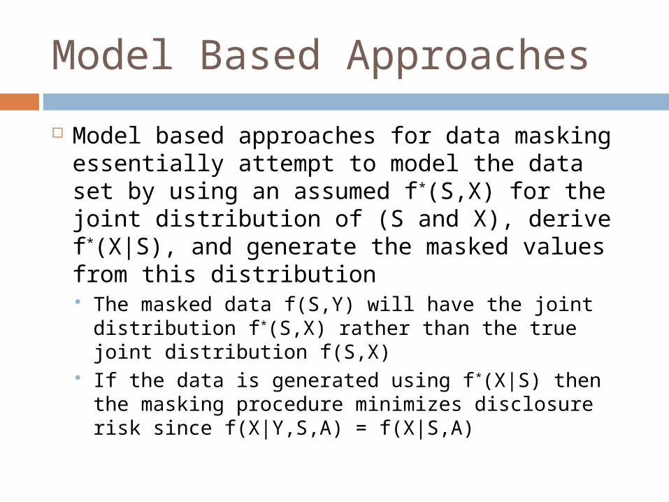
Model based approaches for data masking essentially attempt to model the data set by using an assumed f*(S,X) for the joint distribution of (S and X), derive f*(X|S), and generate the masked values from this distribution The masked data f(S,Y) will have the joint

distribution f*(S,X) rather than the true joint distribution f(S,X)

If the data is generated using f*(X|S) then the masking procedure minimizes disclosure risk since f(X|Y,S,A) = f(X|S,A)

Disclosure risk example

Assume that we have one non-confidential variable S and one confidential variable X

Y = (a × S) + e (where e is the noise term)

We will always get better prediction if we attempt to predict X using S rather than Y (since Y is noisier than S)

Since we have access to both S and Y, and since S would always provide more information about X than Y, an intelligent intruder will always prefer to use S to predict X than Y

More importantly, since Y is a function of S and random noise, once S is used to predict X, including Y will not improve your predictive ability

Model Based Masking Methods Methods that we have developed and I

will be talking about General additive data perturbation Copula based perturbation Data shuffling

Other Methods PRAM Multiple imputation Skew t perturbation

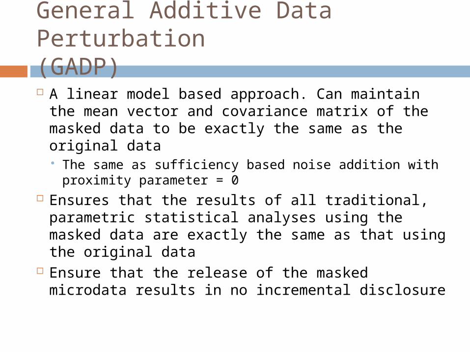
General Additive Data Perturbation(GADP) A linear model based approach. Can maintain the

mean vector and covariance matrix of the masked data to be exactly the same as the original data The same as sufficiency based noise addition with

proximity parameter = 0 Ensures that the results of all traditional,

parametric statistical analyses using the masked data are exactly the same as that using the original data

Ensure that the release of the masked microdata results in no incremental disclosure

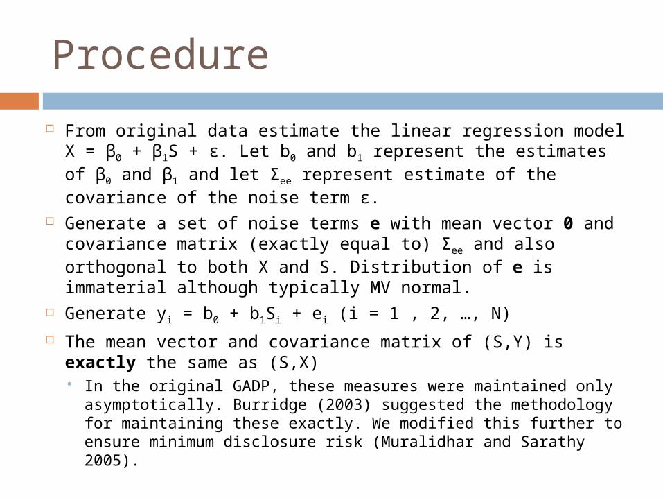
Procedure

From original data estimate the linear regression model X = β0 + β1S + ε. Let b0 and b1 represent the estimates of β0 and β1 and let Σee represent estimate of the covariance of the noise term ε.

Generate a set of noise terms e with mean vector 0 and covariance matrix (exactly equal to) Σee and also orthogonal to both X and S. Distribution of e is immaterial although typically MV normal.

Generate yi = b0 + b1Si + ei (i = 1 , 2, …, N) The mean vector and covariance matrix of (S,Y) is exactly

the same as (S,X) In the original GADP, these measures were maintained only

asymptotically. Burridge (2003) suggested the methodology for maintaining these exactly. We modified this further to ensure minimum disclosure risk (Muralidhar and Sarathy 2005).

Minimum Disclosure Risk

GADP results in minimizing disclosure risk. We can show that an intruder would get the “best estimate” of the confidential values using just the non-confidential variables. The masked variables provide no additional information.

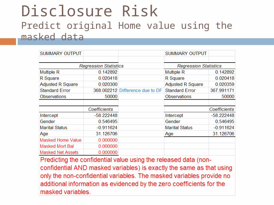
Disclosure RiskPredict original Home value using the masked data

Even if you …

Had say 90% of the entire data set, you would not be able to predict the value of the confidential variables for the remaining 10% with any greater accuracy than you would using only the non-confidential data

Had 100% of all confidential variables except one AND 90% of the values for the last confidential variable, you would not be able to predict the confidential value of remaining records with any greater accuracy than you would using only the non-confidential variables.

(Lack of) Information Loss

By maintaining the mean vector and covariance matrix of the two data sets to be exactly the same, for any statistical analysis for which the mean vector and covariance matrix are sufficient statistics, we ensure that the parameter estimates using the masked data will be exactly the same as the original data

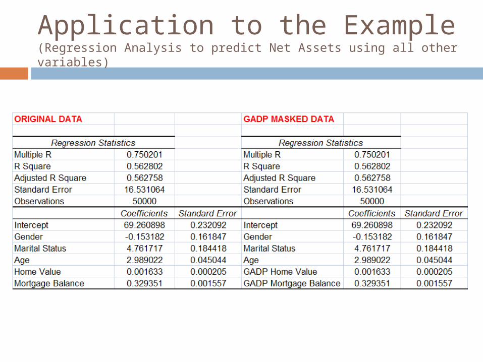
Application to the Example(Regression Analysis to predict Net Assets using all other variables)

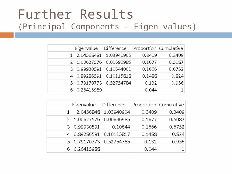
Further Results(Principal Components – Eigen values)

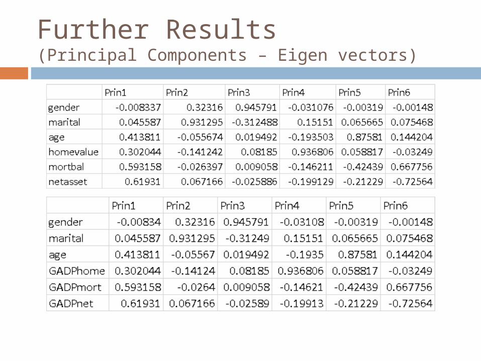
Further Results(Principal Components – Eigen vectors)

But …

Unfortunately, the marginal distribution of the original data set is altered significantly. In most situations, the marginal distribution of the masked variable bears little or no relationship to the original variable The data also could have negative values

when the original variable had only positive values

Marginal Distribution of Home Value

• The change in the marginal distribution means that other analyses pertaining to the distribution of the confidential variables are not maintained– Residual analysis from regression would be very different

Negative values that did not exist

in the original data

Non-Linear Relationships

Since a linear model is used, any non-linear relationships that may have been present in the data are modified (linearized)

GADP … Useful … But …

GADP is useful in a limited context. If the confidential variables do not exhibit significant deviations from normality, then GADP would represent a good solution to the problem

In other cases, GADP represents a limited solution to the specific users who will use the data mainly for traditional statistical analysis

Improving GADP

We would like the masking procedure to provide some additional benefits (while still minimizing disclosure risk) Maintain the marginal distribution Maintain non-linear relationships

To do this, we need to move beyond linear models Multiplicative models are not very useful since,

in essence, they are just variations of the linear model

Copula Based GADP

In statistics, copulas have traditionally been used to model the joint distribution of a set of variables with arbitrary marginal distributions and a specified dependence characteristics

the ability to maintain the marginal, nonnormal distribution of the original attributes to be the same after masking and to preserve certain types of dependence between the attributes

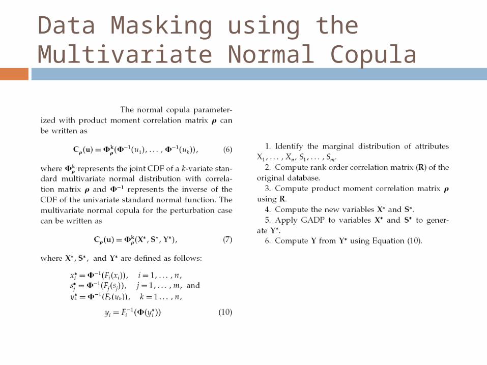
Data Masking using the Multivariate Normal Copula

Characteristics of the C-GADP C-GADP minimizes disclosure risk C-GADP provides the following

information loss characteristics The marginal distribution of the confidential

variables is maintained All monotonic relationships are preserved

Rank order correlation Product moment correlation

Non-monotonic relationships will be modified

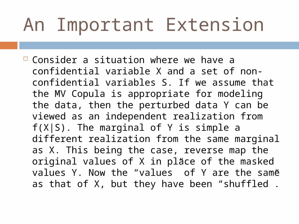
An Important Extension

Consider a situation where we have a confidential variable X and a set of non-confidential variables S. If we assume that the MV Copula is appropriate for modeling the data, then the perturbed data Y can be viewed as an independent realization from f(X|S). The marginal of Y is simple a different realization from the same marginal as X. This being the case, reverse map the original values of X in place of the masked values Y. Now the “values” of Y are the same as that of X, but they have been “shuffled”.

Data Shuffling(US Patent 7200757)

In the above, we use the multivariate normal copula to generate YP.

Characteristics of Data Shuffling Offers all the benefits as CGADP

Minimum disclosure risk Information loss

Maintains the marginal distribution Maintain all monotonic relationships

Additional benefits There is no “modification” of the values. The original

values are used The marginal distribution of the masked data is

exactly the same as the original data Implementation can be performed using only the ranks

A small example

Some shuffled values are far apart, others are closer Impossible to predict

original position after the fact which assures low disclosure risk

Rank order correlation pre and post masking are very close. Improves with the size of the data set

X is less correlated with Y and more correlated with S

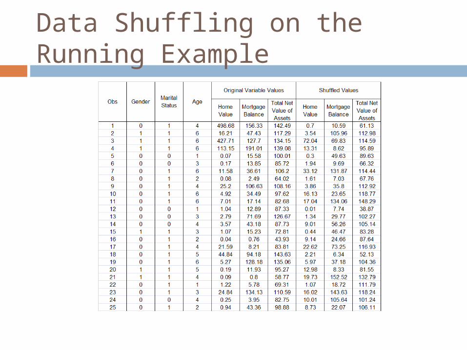
Data Shuffling on the Running Example

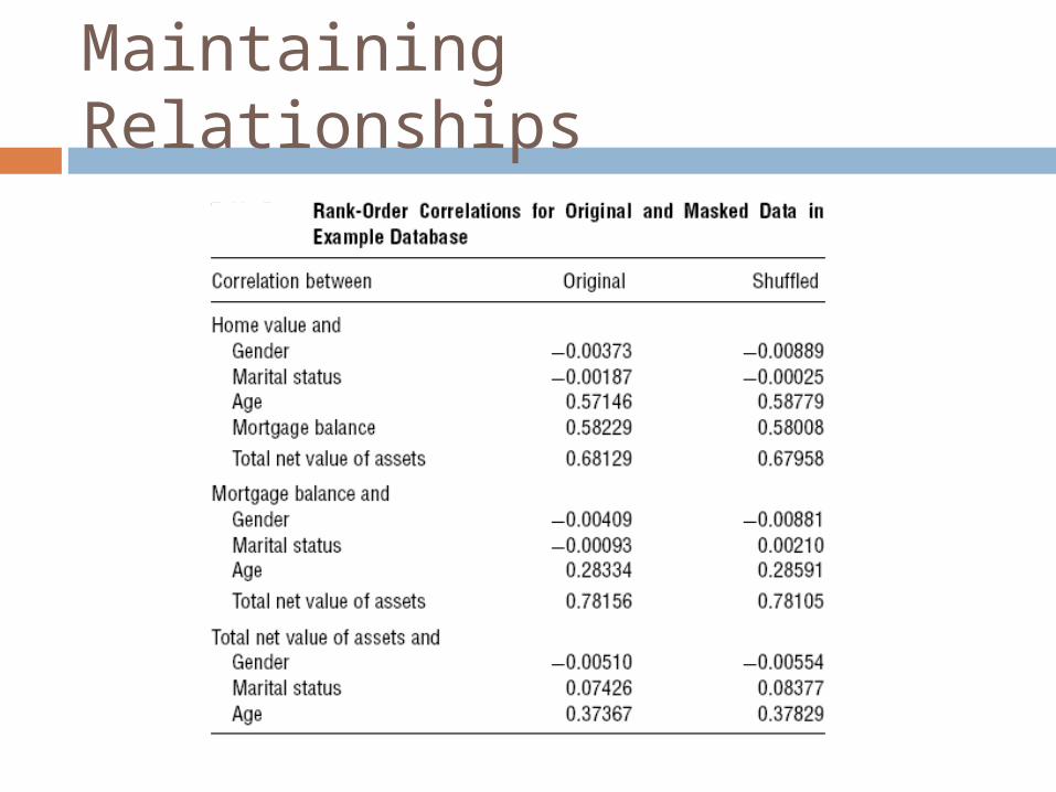
Maintaining Relationships

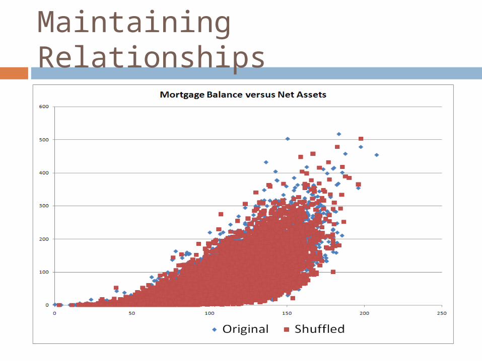
Maintaining Relationships

Advantages of Data Shuffling Data shuffling is a hybrid (perturbation

and swapping), non-parametric (can be implemented only with rank information) technique for data masking that minimizes disclosure risk and offers the lowest level of information loss among existing methods of data masking Will not maintain non-monotonic relationships Does not preserve tail dependence

Can be overcome by using t-copula instead of normal copula

Practically Viable

Data shuffling can be implemented easily even for relatively large data sets. We are in the process of developing two versions of software based on Data shuffling Java based for large applications Excel based for smaller applications

Future Research

Investigate other methods for modeling the joint distribution of the variables to reduce information loss further. Other copula functions? Some other approach?

Investigate non-statistical approaches for producing a masked data set that closely resembles the original data (while minimizing disclosure risk)

Masking methods for discrete numerical data

Some Important References

Dalenius, T., “Towards a methodology for statistical disclosure control,” Statistisktidskrift, 5, 429–444, 1977.

Fuller, W. A., “Masking procedures for microdata disclosure limitation,” Journal of Official Statististics, 9, 383–406, 1993.

Rubin, D. B., “Discussion of statistical disclosure limitation,” Journal of Official Statistics, 9, 461–468, 1993.

Moore, R. A., “Controlled data swapping for masking public use microdata sets,” Research report series no. RR96/04, U.S. Census Bureau, Statistical Research Division, Washington, D.C., 1996.

Burridge, J., “Information preserving statistical obfuscation,” Statistics and Computing, 13, 321–327, 2003.

Domingo-Ferrer, J. and J.M. Mateo-Sanz, “Practical data-oriented microaggregation for statistical disclosure control,” IEEE Transactions on Knowledge and Data Engineering, 14, 189-201, 2002.

Our Publications Relating to Data Masking Muralidhar, K. and R. Sarathy, " Generating Sufficiency-based Non-

Synthetic Perturbed Data," Transactions on Data Privacy, 1(1), 17-33, 2008.

Muralidhar, K. and R. Sarathy, "Data Shuffling- A New Masking Approach for Numerical Data," Management Science, 52(5), 658-670, 2006.

Muralidhar, K. and R. Sarathy, “A Comparison of Multiple Imputation and Data Perturbation for Masking Numerical Variables,” Journal of Official Statistics, 22(3), 507-524, 2006.

Muralidhar, K. and R. Sarathy, " A Theoretical Basis for Perturbation Methods," Statistics and Computing, 13(4), 329-335, 2003.

Sarathy, R., K. Muralidhar, and R. Parsa, "Perturbing Non-Normal Confidential Attributes: The Copula Approach," Management Science, 48(12), 1613-1627, 2002.

Muralidhar, K., R. Parsa, and R. Sarathy, "A General Additive Data Perturbation Method for Database Security," Management Science, 45(10), 1399-1415, 1999.

Muralidhar, K., D. Batra, and P. Kirs, “Accessibility, Security, and Accuracy in Statistical Databases: The Case for the Multiplicative Fixed Data Perturbation Approach,” Management Science, 41(9), 1549-1564,1995.

Other Related Research

Assessing disclosure risk Muralidhar, K. and R. Sarathy, "Security of Random Data

Perturbation Methods," ACM Transactions on Database Systems, 24(4), 487-493, 1999.

Sarathy, R. and K. Muralidhar, "The Security of Confidential Numerical Data in Databases," Information Systems Research, 13(4), 389-403, 2002.

Li, H., K. Muralidhar, and R. Sarathy, “Assessment of Disclosure Risk when using Confidentiality via Camouflage,” Operations Research, 55(6), 1178-1182, 2007.

Framework for evaluating masking techniques Muralidhar, K. and R. Sarathy, “A Theoretical Comparison of

Data Masking Techniques for Numerical Microdata,” to be presented at the 3rd IAB Workshop on Confidentiality and Disclosure - SDC for Microdata, Nuremberg, Germany, 2008

Web Site URL

You can many of our papers and presentations at our web site:

http://gatton.uky.edu/faculty/muralidhar/maskingpapers/

I will be happy to share any papers or presentations that are not available on the web site.

Conclusion

There are a host of techniques that are available for masking numerical data. These techniques have a long history in the statistical disclosure limitation literature. There is considerable overlap between the data masking research in the statistical disclosure limitation research community and the privacy preserving data mining research in the CS community. Unfortunately, there seems to be only a limited cooperation between the researchers in the two fields. I believe that each field can make a significant contribution to the other. I hope that this presentation contributes to enhancing the discussion between CS and SDL researchers … at least at UK.

Questions, Suggestions or

Comments?

Thank you