A Primer on Permutation Tests(not only) for MVPA

Carsten Allefeld

Theory and Analysis of Large-Scale Brain SignalsBernstein Center for Computational Neuroscience

and Charité – Universitätsmedizin, Berlin

introductionwhy use a permutation test?▶ sometimes precise distributions are not known,

especially in MVPA▶ a permutation test makes

weaker assumptions about distributionsthan parametric tests

▶ permutation tests provide exact inference▶ permutation testing applies in the same way

to uni- and multivariate analysis

this talk▶ no recipes, but the basic principles underlying

permutation tests, especially exchangeability

a univariate example: two-sample testis there a mean difference between groups A and B?

original data

A

B

7

6

1

3

4

9

computation

x̄A = 4

x̄B = 6

x̄B − x̄A = 2

test statistic

T = 2

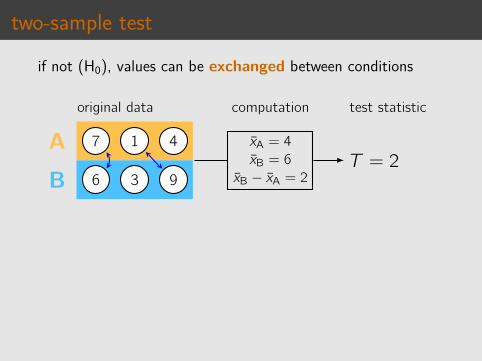
two-sample testif not (H0), values can be exchanged between conditions

original data

A

B

7

6

1

3

4

9

computation

x̄A = 4

x̄B = 6

x̄B − x̄A = 2

test statistic

T = 2

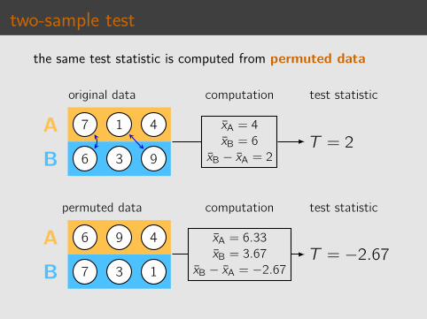
two-sample testthe same test statistic is computed from permuted data

original data

A

B

7

6

1

3

4

9

computation

x̄A = 4

x̄B = 6

x̄B − x̄A = 2

test statistic

T = 2

permuted data

A

B

6

7

9

3

4

1

computation

x̄A = 6.33

x̄B = 3.67

x̄B − x̄A = −2.67

test statistic

T = −2.67

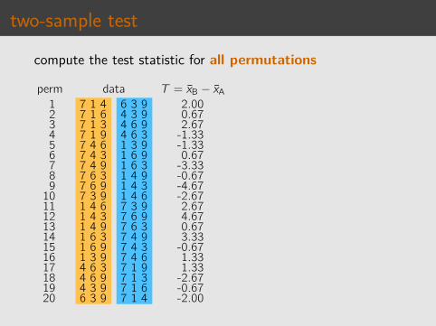
two-sample testcompute the test statistic for all permutations

perm data T = x̄B − x̄A1 7 1 4 6 3 9 2.002 7 1 6 4 3 9 0.673 7 1 3 4 6 9 2.674 7 1 9 4 6 3 -1.335 7 4 6 1 3 9 -1.336 7 4 3 1 6 9 0.677 7 4 9 1 6 3 -3.338 7 6 3 1 4 9 -0.679 7 6 9 1 4 3 -4.67

10 7 3 9 1 4 6 -2.6711 1 4 6 7 3 9 2.6712 1 4 3 7 6 9 4.6713 1 4 9 7 6 3 0.6714 1 6 3 7 4 9 3.3315 1 6 9 7 4 3 -0.6716 1 3 9 7 4 6 1.3317 4 6 3 7 1 9 1.3318 4 6 9 7 1 3 -2.6719 4 3 9 7 1 6 -0.6720 6 3 9 7 1 4 -2.00

two-sample testdetermine ranks by sorting in descending order

perm data T = x̄B − x̄A sorted rank1 7 1 4 6 3 9 2.00 4.67 12 7 1 6 4 3 9 0.67 3.33 23 7 1 3 4 6 9 2.67 2.67 34 7 1 9 4 6 3 -1.33 2.67 45 7 4 6 1 3 9 -1.33 2.00 56 7 4 3 1 6 9 0.67 1.33 67 7 4 9 1 6 3 -3.33 1.33 78 7 6 3 1 4 9 -0.67 0.67 89 7 6 9 1 4 3 -4.67 0.67 9

10 7 3 9 1 4 6 -2.67 0.67 1011 1 4 6 7 3 9 2.67 -0.67 1112 1 4 3 7 6 9 4.67 -0.67 1213 1 4 9 7 6 3 0.67 -0.67 1314 1 6 3 7 4 9 3.33 -1.33 1415 1 6 9 7 4 3 -0.67 -1.33 1516 1 3 9 7 4 6 1.33 -2.00 1617 4 6 3 7 1 9 1.33 -2.67 1718 4 6 9 7 1 3 -2.67 -2.67 1819 4 3 9 7 1 6 -0.67 -3.33 1920 6 3 9 7 1 4 -2.00 -4.67 20

two-sample testthe neutral permutation is part of the set

perm data T = x̄B − x̄A sorted rank1 7 1 4 6 3 9 2.00 4.67 12 7 1 6 4 3 9 0.67 3.33 23 7 1 3 4 6 9 2.67 2.67 34 7 1 9 4 6 3 -1.33 2.67 45 7 4 6 1 3 9 -1.33 2.00 56 7 4 3 1 6 9 0.67 1.33 67 7 4 9 1 6 3 -3.33 1.33 78 7 6 3 1 4 9 -0.67 0.67 89 7 6 9 1 4 3 -4.67 0.67 9

10 7 3 9 1 4 6 -2.67 0.67 1011 1 4 6 7 3 9 2.67 -0.67 1112 1 4 3 7 6 9 4.67 -0.67 1213 1 4 9 7 6 3 0.67 -0.67 1314 1 6 3 7 4 9 3.33 -1.33 1415 1 6 9 7 4 3 -0.67 -1.33 1516 1 3 9 7 4 6 1.33 -2.00 1617 4 6 3 7 1 9 1.33 -2.67 1718 4 6 9 7 1 3 -2.67 -2.67 1819 4 3 9 7 1 6 -0.67 -3.33 1920 6 3 9 7 1 4 -2.00 -4.67 20

two-sample testthe rank of the original value determines significance

perm data T = x̄B − x̄A sorted rank1 7 1 4 6 3 9 2.00 4.67 12 7 1 6 4 3 9 0.67 3.33 23 7 1 3 4 6 9 2.67 2.67 34 7 1 9 4 6 3 -1.33 2.67 45 7 4 6 1 3 9 -1.33 2.00 56 7 4 3 1 6 9 0.67 1.33 67 7 4 9 1 6 3 -3.33 1.33 78 7 6 3 1 4 9 -0.67 0.67 89 7 6 9 1 4 3 -4.67 0.67 9

10 7 3 9 1 4 6 -2.67 0.67 1011 1 4 6 7 3 9 2.67 -0.67 1112 1 4 3 7 6 9 4.67 -0.67 1213 1 4 9 7 6 3 0.67 -0.67 1314 1 6 3 7 4 9 3.33 -1.33 1415 1 6 9 7 4 3 -0.67 -1.33 1516 1 3 9 7 4 6 1.33 -2.00 1617 4 6 3 7 1 9 1.33 -2.67 1718 4 6 9 7 1 3 -2.67 -2.67 1819 4 3 9 7 1 6 -0.67 -3.33 1920 6 3 9 7 1 4 -2.00 -4.67 20

significant

two-sample testequivalently, a p-value can be computed

perm data T = x̄B − x̄A sorted rank1 7 1 4 6 3 9 2.00 4.67 12 7 1 6 4 3 9 0.67 3.33 23 7 1 3 4 6 9 2.67 2.67 34 7 1 9 4 6 3 -1.33 2.67 45 7 4 6 1 3 9 -1.33 2.00 56 7 4 3 1 6 9 0.67 1.33 67 7 4 9 1 6 3 -3.33 1.33 78 7 6 3 1 4 9 -0.67 0.67 89 7 6 9 1 4 3 -4.67 0.67 9

10 7 3 9 1 4 6 -2.67 0.67 1011 1 4 6 7 3 9 2.67 -0.67 1112 1 4 3 7 6 9 4.67 -0.67 1213 1 4 9 7 6 3 0.67 -0.67 1314 1 6 3 7 4 9 3.33 -1.33 1415 1 6 9 7 4 3 -0.67 -1.33 1516 1 3 9 7 4 6 1.33 -2.00 1617 4 6 3 7 1 9 1.33 -2.67 1718 4 6 9 7 1 3 -2.67 -2.67 1819 4 3 9 7 1 6 -0.67 -3.33 1920 6 3 9 7 1 4 -2.00 -4.67 20

significant

p = 520 = 0.25

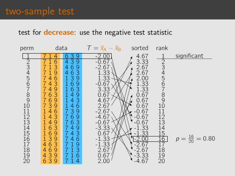
two-sample testtest for decrease: use the negative test statistic

perm data T = x̄A − x̄B sorted rank1 7 1 4 6 3 9 -2.00 4.67 12 7 1 6 4 3 9 -0.67 3.33 23 7 1 3 4 6 9 -2.67 2.67 34 7 1 9 4 6 3 1.33 2.67 45 7 4 6 1 3 9 1.33 2.00 56 7 4 3 1 6 9 -0.67 1.33 67 7 4 9 1 6 3 3.33 1.33 78 7 6 3 1 4 9 0.67 0.67 89 7 6 9 1 4 3 4.67 0.67 9

10 7 3 9 1 4 6 2.67 0.67 1011 1 4 6 7 3 9 -2.67 -0.67 1112 1 4 3 7 6 9 -4.67 -0.67 1213 1 4 9 7 6 3 -0.67 -0.67 1314 1 6 3 7 4 9 -3.33 -1.33 1415 1 6 9 7 4 3 0.67 -1.33 1516 1 3 9 7 4 6 -1.33 -2.00 1617 4 6 3 7 1 9 -1.33 -2.67 1718 4 6 9 7 1 3 2.67 -2.67 1819 4 3 9 7 1 6 0.67 -3.33 1920 6 3 9 7 1 4 2.00 -4.67 20

significant

p = 1620 = 0.80

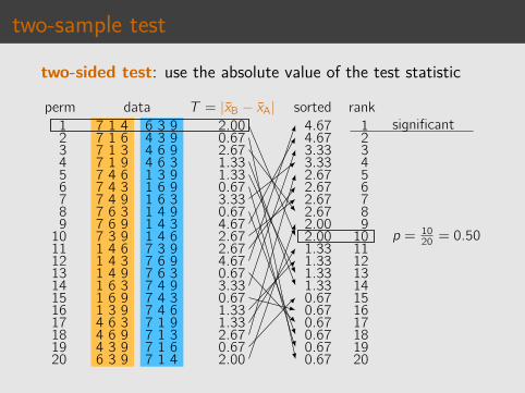
two-sample testtwo-sided test: use the absolute value of the test statistic

perm data T = |x̄B − x̄A| sorted rank1 7 1 4 6 3 9 2.00 4.67 12 7 1 6 4 3 9 0.67 4.67 23 7 1 3 4 6 9 2.67 3.33 34 7 1 9 4 6 3 1.33 3.33 45 7 4 6 1 3 9 1.33 2.67 56 7 4 3 1 6 9 0.67 2.67 67 7 4 9 1 6 3 3.33 2.67 78 7 6 3 1 4 9 0.67 2.67 89 7 6 9 1 4 3 4.67 2.00 9

10 7 3 9 1 4 6 2.67 2.00 1011 1 4 6 7 3 9 2.67 1.33 1112 1 4 3 7 6 9 4.67 1.33 1213 1 4 9 7 6 3 0.67 1.33 1314 1 6 3 7 4 9 3.33 1.33 1415 1 6 9 7 4 3 0.67 0.67 1516 1 3 9 7 4 6 1.33 0.67 1617 4 6 3 7 1 9 1.33 0.67 1718 4 6 9 7 1 3 2.67 0.67 1819 4 3 9 7 1 6 0.67 0.67 1920 6 3 9 7 1 4 2.00 0.67 20

significant

p = 1020 = 0.50

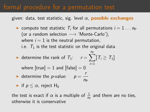
formal procedure for a permutation testgiven: data, test statistic, sig. level α, possible exchanges

▶ compute test statistic Ti for all permutations i = 1 . . . nP(or a random selection −→ ‘Monte-Carlo’),where i = 1 is the neutral permutation,i.e. T1 is the test statistic on the original data

▶ determine the rank of T1: r =nP∑i=1

[Ti ≥ T1]

where [true] = 1 and [false] = 0▶ determine the p-value: p =

rnP

▶ if p ≤ α, reject H0

the test is exact if α is a multiple of 1nP

and there are no ties,otherwise it is conservative

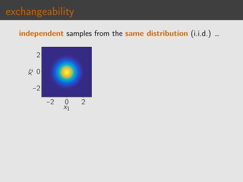
exchangeabilityindependent samples from the same distribution (i.i.d.) …

−2 0 2

−2

0

2

x1

x 2

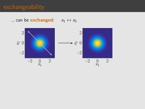
exchangeability… can be exchanged: x1 ↔ x2

−2 0 2

−2

0

2

x1

x 2

−2 0 2

−2

0

2

x1

x 2

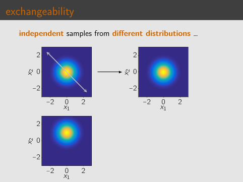
exchangeabilityindependent samples from different distributions …

−2 0 2

−2

0

2

x1

x 2

−2 0 2

−2

0

2

x1

x 2

−2 0 2

−2

0

2

x1

x 2

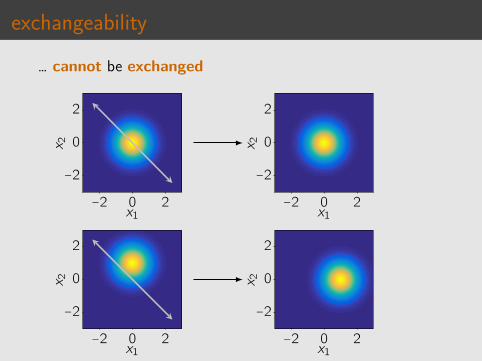
exchangeability… cannot be exchanged

−2 0 2

−2

0

2

x1

x 2

−2 0 2

−2

0

2

x1

x 2

−2 0 2

−2

0

2

x1

x 2

−2 0 2

−2

0

2

x1

x 2

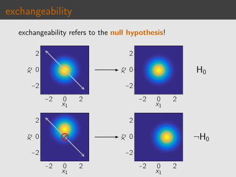
exchangeabilityexchangeability refers to the null hypothesis!

−2 0 2

−2

0

2

x1

x 2

−2 0 2

−2

0

2

x1

x 2 H0

−2 0 2

−2

0

2

x1

x 2

−2 0 2

−2

0

2

x1

x 2 ¬H0

exchangeabilityexchangeable also if there is dependency but symmetric

−2 0 2

−2

0

2

x1

x 2

−2 0 2

−2

0

2

x1

x 2 H0

−2 0 2

−2

0

2

x1

x 2

−2 0 2

−2

0

2

x1

x 2 ¬H0

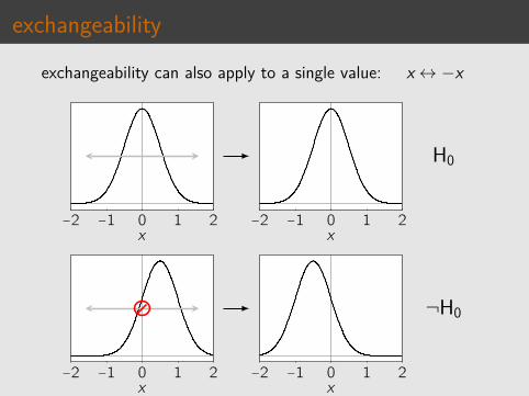
exchangeabilityexchangeability can also apply to a single value: x↔ −x

−2 −1 0 1 2x

−2 −1 0 1 2x

H0

−2 −1 0 1 2x

−2 −1 0 1 2x

¬H0

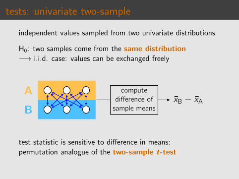
tests: univariate two-sampleindependent values sampled from two univariate distributions

H0: two samples come from the same distribution−→ i.i.d. case: values can be exchanged freely

A

B

computedifference ofsample means

x̄B − x̄A

test statistic is sensitive to difference in means:permutation analogue of the two-sample t-test

tests: multivariate two-sampleindependently sampled from two multivariate distributions

H0: two samples from the same multivariate distribution−→ i.i.d. case: vector values can be exchanged freely

A

B

train andtest classifier,cross-validated

accuracy

Problem with accuracies: few possible values −→ ties!

Example: classification of subject-specific patterns,e.g. of patients based on structural MRI

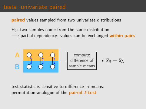
tests: univariate pairedpaired values sampled from two univariate distributions

H0: two samples come from the same distribution−→ partial dependency: values can be exchanged within pairs

A

B

computedifference ofsample means

x̄B − x̄A

test statistic is sensitive to difference in means:permutation analogue of the paired t-test

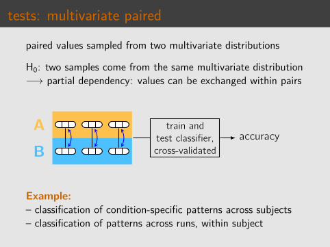
tests: multivariate pairedpaired values sampled from two multivariate distributions

H0: two samples come from the same multivariate distribution−→ partial dependency: values can be exchanged within pairs

A

B

train andtest classifier,cross-validated

accuracy

Example:– classification of condition-specific patterns across subjects– classification of patterns across runs, within subject

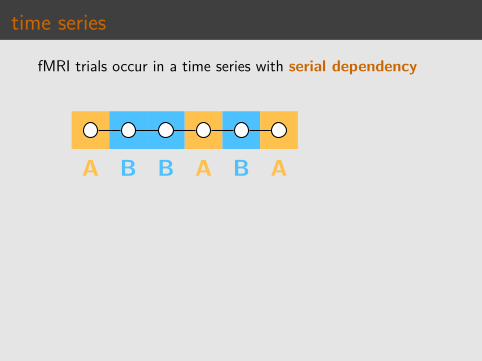
time seriesfMRI trials occur in a time series with serial dependency

A B B A B A

time seriesproblem: exchanges change the dependency structure

A B B A B A

A B B A B A

time seriesno exchangeability of values in fMRI time series!

A B B A B A

A B B A B A

time seriesfor a randomized trial sequence, labels can be exchanged

A B B A B A

−→ randomization test, ̸= permutation testdisadvantage: weaker inference

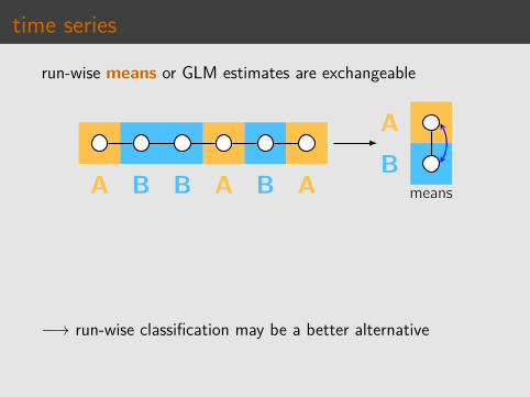
time seriesrun-wise means or GLM estimates are exchangeable

A B B A B A

A

Bmeans

−→ run-wise classification may be a better alternative

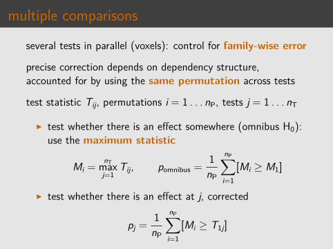
multiple comparisonsseveral tests in parallel (voxels): control for family-wise error

precise correction depends on dependency structure,accounted for by using the same permutation across tests

test statistic Tij, permutations i = 1 . . . nP, tests j = 1 . . . nT

▶ test whether there is an effect somewhere (omnibus H0):use the maximum statistic

Mi =nTmaxj=1

Tij, pomnibus =1nP

nP∑i=1

[Mi ≥ M1]

▶ test whether there is an effect at j, corrected

pj =1nP

nP∑i=1

[Mi ≥ T1j]

further readinggeneral– Ernst, Permutation methods: A basis for exact inference, Statistical Science 2004– Good, Permutation, Parametric, and Bootstrap Tests of Hypotheses, Springer 2005– Lehmann & Romano, Testing Statistical Hypotheses, Springer 2005, Sec. 5.8

neuroimaging– Nichols & Holmes, Nonparametric permutation tests for functional neuroimaging: A

primer with examples, Human Brain Mapping 2001– Winkler et al., Permutation inference for the general linear model, NeuroImage 2014– Winkler et al., Multi-level block permutation, NeuroImage 2015

MVPA– Golland & Fischl, Permutation tests for classification: Towards statistical

significance in image-based studies, Information processing in medical imaging 2003– Etzel & Braver, MVPA permutation schemes: Permutation testing in the land of

cross-validation, PRNI 2013– Schreiber & Krekelberg, The statistical analysis of multi-voxel patterns in functional

imaging, PLOS ONE 2013– Stelzer, Chen, Turner, Statistical inference and multiple testing correction in

classification-based multi-voxel pattern analysis (MVPA), NeuroImage 2013

see me at poster 2159, Tuesday, 12:45–14:45Valid population inference for information-based imaging