a probabilistic and non-deterministic call-by-push …
TRANSCRIPT

A PROBABILISTIC AND NON-DETERMINISTIC CALL-BY-PUSH-VALUE LANGUAGEJean Goubault-Larrecq

PCF, probabilistic choice, and the trouble with V
Curing the trouble using call-by-push-value
Semantics, adequacy, full abstraction

Theoretical Computer Science 5 (1977) 223-255. @ Korth-Holland Publishi
. iv Department of Artificial Intelligence, University of Edinburgh, Hope Park Square, Meadow Lane,
dinburgh EH8 9NW, Scotland
Communicated by Robin Milner Received July 1975
Abstract. The paper studies connections between denotational and operational semantics for a simple programming language based on LCF. It begins with the connection between the behaviour of a program and its denotation. It turns out that a program denotes _L in any of severai possible semantics iff it does not terminate. From this it follows that if two terms have the same denotation in one of these semantics, they have the same behaviour in all contexts. The converse fails for all the semantics. If, however, the language is extended to allow certain parallel facilities, behaviours: equivalence does coincide with denotational equivalence in one of the semantics1 considered, which may therefore be called “fully abstract”. Next a connection is given which actually determines -he semantics up to isomorphism from the behaviour alone. Conversely, by allowing further parallel facilities, every r.e. element of the fully abstract semantic?, becomes definable, thus characterising the programming language, up to interdefinability, from the set of r.e. elements of he domains of the semantics.
We present here a study of some connections between the operational and denotational semantics of a simple programming language based on LCF [3,5].
bile this language is. itself rather far from the commonly used languages, we do hop,- that the kind o connections studied will be illuminating in the study of these
ature of its denotatdon. For us a program will b
223
PLOTKIN’S PCF (1977)
Types σ, τ, … ::= int | σ → τ
Terms M, N, … ::= xτ | MN | λ xσ . M | rec xσ . M | n | succ M | pred M | ifz M N P
(All terms are typed. Call by name.)

PLOTKIN’S PCF (1977)
An operational semantics: M →* N
A denotational semantics: ⟦M⟧
Adequacy: for every ground M : int, ⟦M⟧=n iff M →* n
Types σ, τ, … ::= int | σ → τ
Terms M, N, … ::= xτ | MN | λ xσ . M | rec xσ . M | n | succ M | pred M | ifz M N P
(All terms are typed. Call by name.)

PLOTKIN’S PCF (1977)
Contextual preordering: M ⪯ N iff for every context C : int, C[M] →* n ⇒ C[N] →* n
Fact: if ⟦M⟧≤⟦N⟧ then M ⪯ N
Converse is full abstraction. Fails for PCF, works for PCF+por
An operational semantics: M →* N
A denotational semantics: ⟦M⟧
Adequacy: for every ground M : int, ⟦M⟧=n iff M →* n

DCPOS
Every type τ interpreted as a dcpo ⟦τ⟧⋁D
D
A directed family D. In a dcpo, every directed family D has a supremum ⋁D

DCPOS
Every type τ interpreted as a dcpo ⟦τ⟧
⟦int⟧ = ℤ⊥ (⊥≤n, all n incomparable)
⋁D
D
A directed family D. In a dcpo, every directed family D has a supremum ⋁D

DCPOS
Every type τ interpreted as a dcpo ⟦τ⟧
⟦int⟧ = ℤ⊥ (⊥≤n, all n incomparable)
⟦σ → τ⟧ = [⟦σ⟧ → ⟦τ⟧], dcpo of Scott-continuous maps : ⟦σ⟧ → ⟦τ⟧ (monotonic + preserves directed sups)
⋁D
D
A directed family D. In a dcpo, every directed family D has a supremum ⋁D

THE SEMANTICS OF PCF
⟦MN⟧ = ⟦M⟧(⟦N⟧) ⟦λ xσ . M⟧ = (V ↦ ⟦M⟧[xσ:=V])
Meaningful since Dcpo is a Cartesian-closed category
Types σ, τ, … ::= int | σ → τ
Terms M, N, … ::= xτ | MN | λ xσ . M | rec xσ . M | n | succ M | pred M | ifz M N P
∈ ⟦σ → τ⟧ ∈ ⟦σ⟧
∈ ⟦σ⟧ ∈ ⟦τ⟧

⟦MN⟧ = ⟦M⟧(⟦N⟧) ⟦λ xσ . M⟧ = (V ↦ ⟦M⟧[xσ:=V])
Meaningful since Dcpo is a Cartesian-closed category
CARTESIAN-CLOSEDNESS
In order to prove full abstraction (with por), we require to be able to approximate elements of ⟦τ⟧ by definable elements ⟦M⟧.
In the case of PCF, each ⟦τ⟧ is an algebraic bc-domain, making that possible.
Cartesian-closed… good.
∈ ⟦σ → τ⟧ ∈ ⟦σ⟧
∈ ⟦σ⟧ ∈ ⟦τ⟧

CCCS OF CONTINUOUS DCPOS
In order to prove full abstraction (with por), we require to be able to approximate elements of ⟦τ⟧ by definable elements ⟦M⟧.
In the case of PCF, each ⟦τ⟧ is an algebraic bc-domain, making that possible.
Cartesian-closed… good. algebraicbc-domains

CCCS OF CONTINUOUS DCPOS
In order to prove full abstraction (with por), we require to be able to approximate elements of ⟦τ⟧ by definable elements ⟦M⟧.
In the case of PCF, each ⟦τ⟧ is an algebraic bc-domain, making that possible.
Cartesian-closed… good.
Many other CCCs would fit, provided they consist of continuous dcpos.
algebraicbc-domains
bc-domains
algebraic complete lattices
continuous complete lattices
bifinite domains
RB-domains
FS-domains
L-domains
continuous coherent dcpos
continuous dcpos
dcpos
CCCs ofcontinuous
dcpos

ADDING PROBABILITIES
Typesσ, τ, … ::= int | σ → τ | Vτ
Terms M, N, … ::= … | M ⊕ N | ret M | do xσ ⃪ M; N

ADDING PROBABILITIES
Typesσ, τ, … ::= int | σ → τ | Vτ
Terms M, N, … ::= … | M ⊕ N | ret M | do xσ ⃪ M; N
Monadic type of subprobability valuations over τ

ADDING PROBABILITIES
Typesσ, τ, … ::= int | σ → τ | Vτ
Terms M, N, … ::= … | M ⊕ N | ret M | do xσ ⃪ M; N
Monadic type of subprobability valuations over τ
with M, N: Vτ,choose between M and N
with probability 1/2

ADDING PROBABILITIES
Typesσ, τ, … ::= int | σ → τ | Vτ
Terms M, N, … ::= … | M ⊕ N | ret M | do xσ ⃪ M; N
Monadic type of subprobability valuations over τ
with M, N: Vτ,choose between M and N
with probability 1/2
monadic constructions:M:τ ⇒ ret M:Vτ
M:Vσ N:Vτ ⇒ do xσ ⃪ M; N : Vτ
(Moggi 1991)

THE TROUBLE WITH V
algebraicbc-domains
bc-domains
algebraic complete lattices
continuous complete lattices
bifinite domains
RB-domains
FS-domains
L-domains
continuous coherent dcpos
continuous dcpos
Look for a category of continuous dcpos that is…
(Jung, Tix 1998)

THE TROUBLE WITH V
algebraicbc-domains
bc-domains
algebraic complete lattices
continuous complete lattices
bifinite domains
RB-domains
FS-domains
L-domains
continuous coherent dcpos
continuous dcpos
Look for a category of continuous dcpos that is…
Cartesian-closed
(Jung, Tix 1998)

THE TROUBLE WITH V
algebraicbc-domains
bc-domains
algebraic complete lattices
continuous complete lattices
bifinite domains
RB-domains
FS-domains
L-domains
continuous coherent dcpos
continuous dcpos
Look for a category of continuous dcpos that is…
Cartesian-closed
closed under V
?
?(Jung, Tix 1998)

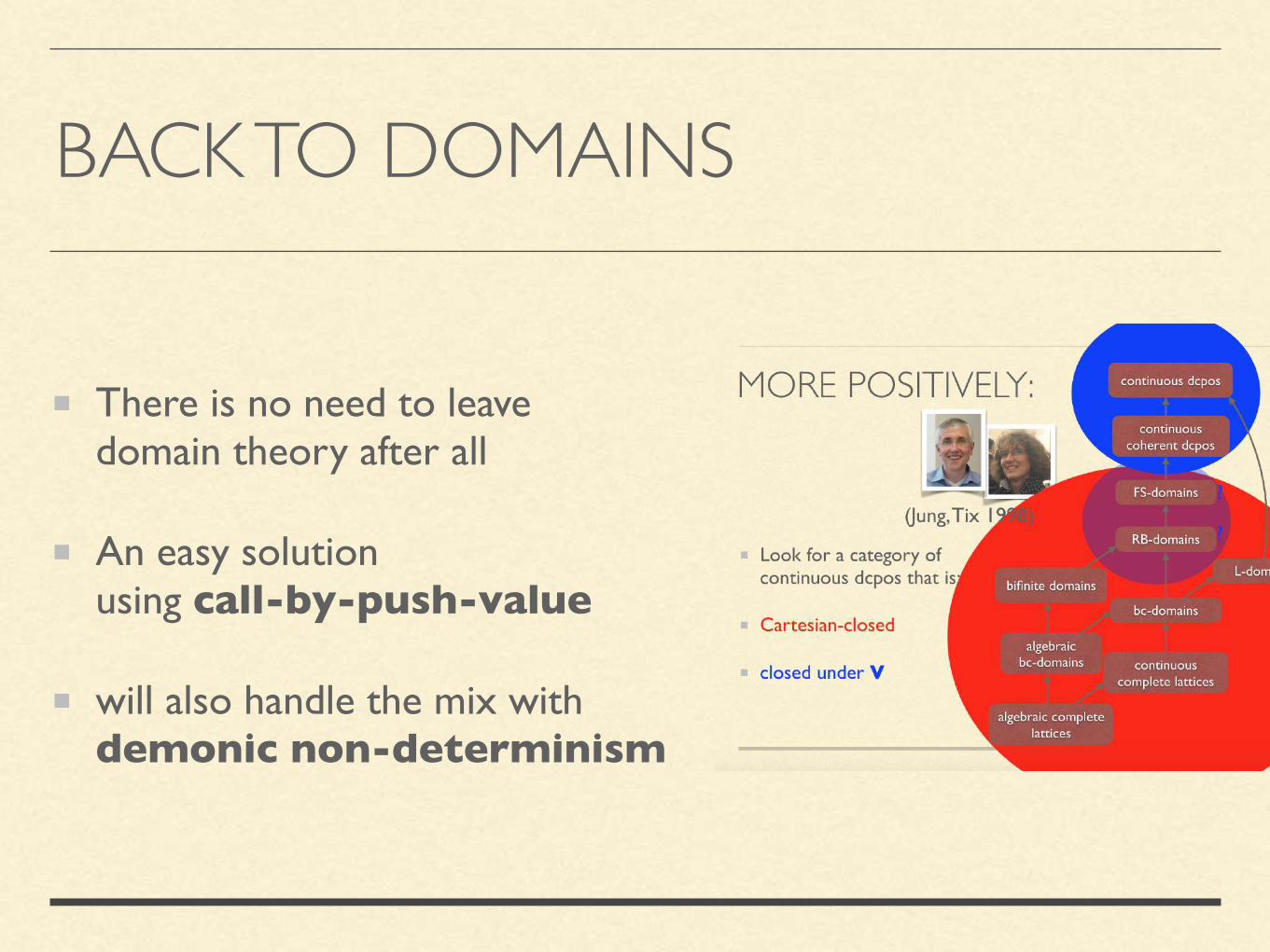
MORE POSITIVELY:
algebraicbc-domains
bc-domains
algebraic complete lattices
continuous complete lattices
bifinite domains
RB-domains
FS-domains
L-domains
continuous coherent dcpos
continuous dcpos
Look for a category of continuous dcpos that is:
Cartesian-closed
closed under V
(Jung, Tix 1998)

MORE POSITIVELY:
algebraicbc-domains
bc-domains
algebraic complete lattices
continuous complete lattices
bifinite domains
RB-domains
FS-domains
L-domains
continuous coherent dcpos
continuous dcpos
Look for a category of continuous dcpos that is:
Cartesian-closed
closed under V
?
?(Jung, Tix 1998)

OTHER SOLUTIONS (1)
Change categories entirely. E.g., reason in probabilistic coherence spaces
Equationally fully abstract semantics(Ehrhard, Pagani, Tasson 14)
also for call-by-push-value (Ehrhard, Tasson 19)
probabilistic choice ‘built-in’

OTHER SOLUTIONS (2)
Change categories, and opt for QCB spaces/predomains (Battenfeld 06) … Cartesian-closed, and has a probabilistic choice monad

OTHER SOLUTIONS (2)
Change categories, and opt for QCB spaces/predomains (Battenfeld 06) … Cartesian-closed, and has a probabilistic choice monad
Changes categories, and opt for quasi-Borel spaces/domains (Heunen, Kammar, Staton, Yang 17; Vákár, Kammar, Staton 19) … Cartesian-closed, and closed under a ‘laws of random variables’ functor
BACK TO DOMAINS
There is no need to leave domain theory after all
An easy solutionusing call-by-push-value
will also handle the mix with demonic non-determinism

PCF, probabilistic choice, and the trouble with V
Curing the trouble using call-by-push-value
Semantics, adequacy, full abstraction

PCF, probabilistic choice, and the trouble with V
Curing the trouble using call-by-push-value
Semantics, adequacy, full abstraction

TWO KINDS OF TYPES?
No such problem with two kinds of types: σ, τ, … ::= int | … | σ × τ | Vτσ, τ, … ::= … | σ → τ
continuous (coherent) dcpos
bc-domains/continuous lattices

CALL-BY-PUSH-VALUE
No such problem with two kinds of types: σ, τ, … ::= int | unit | Uσ | σ × τ | Vτσ, τ, … ::= Fσ | σ → τ
This is the type structure of Paul B. Levy’s call-by-push-value (except for the V construction)
(Levy 1999)
continuous (coherent) dcpos
bc-domains/continuous lattices

CALL-BY-PUSH-VALUE
No such problem with two kinds of types: σ, τ, … ::= int | unit | Uσ | σ × τ | Vτσ, τ, … ::= Fσ | σ → τ
This is the type structure of Paul B. Levy’s call-by-push-value (except for the V construction)
(Levy 1999)
continuous (coherent) dcpos
bc-domains/continuous lattices
value types
computation types

U AND F
σ, τ, … ::= int | unit | σ × τ | Vτσ, τ, … ::= σ → τ
continuous (coherent) dcpos
bc-domains/continuous lattices

U AND F
σ, τ, … ::= int | unit | Uσ | σ × τ | Vτσ, τ, … ::= σ → τ
U converts from bc-domains to continuous coherent dcpos… semantically the identity: ⟦Uσ⟧=⟦σ⟧
continuous (coherent) dcpos
bc-domains/continuous lattices

U AND F
σ, τ, … ::= int | unit | Uσ | σ × τ | Vτσ, τ, … ::= σ → τ
U converts from bc-domains to continuous coherent dcpos… semantically the identity: ⟦Uσ⟧=⟦σ⟧
M, N, … ::= … | force M (Uσ ↝ σ) | thunk M (σ ↝ Uσ)
continuous (coherent) dcpos
bc-domains/continuous lattices

U AND F
σ, τ, … ::= int | unit | Uσ | σ × τ | Vτσ, τ, … ::= σ → τ
U converts from bc-domains to continuous coherent dcpos… semantically the identity: ⟦Uσ⟧=⟦σ⟧
M, N, … ::= … | force M (Uσ ↝ σ) | thunk M (σ ↝ Uσ)
⟦force M⟧ = ⟦M⟧⟦thunk M⟧ = ⟦M⟧
force thunk M → M
continuous (coherent) dcpos
bc-domains/continuous lattices

U AND F
σ, τ, … ::= int | unit | Uσ | σ × τ | Vτσ, τ, … ::= Fσ | σ → τ
U converts from bc-domains to continuous coherent dcpos… semantically the identity: ⟦Uσ⟧=⟦σ⟧
F converts from continuous coherent dcpos to bc-domains… we take ⟦Fσ⟧=(lifted) Smyth powerdomain of ⟦σ⟧
continuous (coherent) dcpos
bc-domains/continuous lattices
THE SMYTH POWERDOMAIN
QX = {compact saturated subsets of X}, reverse inclusion ⊇
QX is a continuous complete lattice for every continuous coherent dcpo X
Serves as a model of demonic non-determinism.

THE SMYTH POWERDOMAIN
QX = {compact saturated subsets of X}, reverse inclusion ⊇ defines a(nother) monad on the cat. of cont. coh. dcpos.
Unit: η : X → QX : x ↦ ↑x (continuous)
Extension: for f : X → L where L continuous complete lattice, let f* : QX → L : Q ↦ inf {f(x) | x ∈ Q}— if f is continuous then f* is continuous— f* o η = f— f* o g* = (f* o g)*

THE SMYTH⊥ POWERDOMAIN
Technically, we use Q⊥X = QX plus a fresh bottom ⊥ … allows f* to be strict now (needed for adequacy)

U AND F
σ, τ, … ::= int | unit | Uσ | σ × τ | Vτσ, τ, … ::= Fσ | σ → τ
U converts from bc-domains to continuous coherent dcpos: ⟦Uσ⟧=⟦σ⟧
F converts from continuous coherent dcpos to bc-domains: ⟦Fσ⟧=Q⊥⟦σ⟧
continuous complete lattices
continuous (coherent) dcpos

U AND F
σ, τ, … ::= int | unit | Uσ | σ × τ | Vτσ, τ, … ::= Fσ | σ → τ
U converts from bc-domains to continuous coherent dcpos: ⟦Uσ⟧=⟦σ⟧
F converts from continuous coherent dcpos to bc-domains: ⟦Fσ⟧=Q⊥⟦σ⟧
continuous complete lattices
M, N, … ::= … | abortFσ | M N | produce M (σ ↝ Fσ) | M to xσ in N
continuous (coherent) dcpos
choice
monad
Jx�K ⇢ = ⇢(x�)
J�x�.MK ⇢ = V 2 J�K 7! JMK (⇢[x� 7! V ]) JMNK ⇢ = JMK ⇢(JNK ⇢)JproduceproduceproduceMK ⇢ = ⌘Q(JMK ⇢)
JM tototo x� ininin NK ⇢ = (V 2 J�K 7! JNK ⇢[x� 7! V ])⇤(JMK ⇢)JthunkthunkthunkMK ⇢ = JMK ⇢ JforceforceforceMK ⇢ = JMK ⇢
J⇤K ⇢ = > JnK ⇢ = n
JsuccsuccsuccMK ⇢ =
⇢n+ 1 if n = JMK ⇢ 6= ?? otherwise
JpredpredpredMK ⇢ =
⇢n� 1 if n = JMK ⇢ 6= ?? otherwise
Jifzifzifz M N P K ⇢ =
8<
:
JNK ⇢ if JMK ⇢ = 0JP K ⇢ if JMK ⇢ 6= 0,?? if JMK ⇢ = ?
JM ;NK ⇢ =
⇢JNK ⇢ if JMK ⇢ = >? otherwise
J⇡1MK ⇢ = m, J⇡2MK ⇢ = n where JMK ⇢ = (m,n)
JhM,NiK ⇢ = (JMK ⇢, JNK ⇢)JretretretMK ⇢ = �JMK⇢
Jdododox� M ;NK ⇢ = (V 2 J�K 7! JNK ⇢[x� 7! V ])†(JMK ⇢)
JM �NK ⇢ =1
2(JMK ⇢+ JNK ⇢)
JM ? NK ⇢ = JMK ⇢ ^ JNK ⇢ JabortabortabortFFF⌧ K ⇢ = ;
Jrecrecrecx�.MK ⇢ = lfp(V 2 J�K 7! JMK ⇢[x� 7! V ])
Jpifzpifzpifz M N P K ⇢ =
8<
:
JNK ⇢ if JMK ⇢ = 0JP K ⇢ if JMK ⇢ 6= 0,?JNK ⇢ ^ JP K ⇢ if JMK ⇢ = ?
J�>bMK ⇢ =
8<
:
> if JMK ⇢ 6= ? andb⌧ ⌫({>}) for every ⌫ 2 JMK ⇢
? otherwise
Figure 2: Denotational semantics
10

U AND F
σ, τ, … ::= int | unit | Uσ | σ × τ | Vτσ, τ, … ::= Fσ | σ → τ
U converts from bc-domains to continuous coherent dcpos: ⟦Uσ⟧=⟦σ⟧
F converts from continuous coherent dcpos to bc-domains: ⟦Fσ⟧=Q⊥⟦σ⟧
continuous complete lattices
M, N, … ::= … | abortFσ | M N | produce M (σ ↝ Fσ) | M to xσ in N
⟦abortFσ⟧ = ∅ ⟦M N⟧ = ⟦M⟧ ⋀ ⟦N⟧⟦produce M⟧ = η(⟦M⟧) ⟦M to xσ in N⟧ = (V ↦ ⟦N⟧[xσ:=V])* (⟦M⟧)
continuous (coherent) dcpos
choice
monad
Jx�K ⇢ = ⇢(x�)
J�x�.MK ⇢ = V 2 J�K 7! JMK (⇢[x� 7! V ]) JMNK ⇢ = JMK ⇢(JNK ⇢)JproduceproduceproduceMK ⇢ = ⌘Q(JMK ⇢)
JM tototo x� ininin NK ⇢ = (V 2 J�K 7! JNK ⇢[x� 7! V ])⇤(JMK ⇢)JthunkthunkthunkMK ⇢ = JMK ⇢ JforceforceforceMK ⇢ = JMK ⇢
J⇤K ⇢ = > JnK ⇢ = n
JsuccsuccsuccMK ⇢ =
⇢n+ 1 if n = JMK ⇢ 6= ?? otherwise
JpredpredpredMK ⇢ =
⇢n� 1 if n = JMK ⇢ 6= ?? otherwise
Jifzifzifz M N P K ⇢ =
8<
:
JNK ⇢ if JMK ⇢ = 0JP K ⇢ if JMK ⇢ 6= 0,?? if JMK ⇢ = ?
JM ;NK ⇢ =
⇢JNK ⇢ if JMK ⇢ = >? otherwise
J⇡1MK ⇢ = m, J⇡2MK ⇢ = n where JMK ⇢ = (m,n)
JhM,NiK ⇢ = (JMK ⇢, JNK ⇢)JretretretMK ⇢ = �JMK⇢
Jdododox� M ;NK ⇢ = (V 2 J�K 7! JNK ⇢[x� 7! V ])†(JMK ⇢)
JM �NK ⇢ =1
2(JMK ⇢+ JNK ⇢)
JM ? NK ⇢ = JMK ⇢ ^ JNK ⇢ JabortabortabortFFF⌧ K ⇢ = ;
Jrecrecrecx�.MK ⇢ = lfp(V 2 J�K 7! JMK ⇢[x� 7! V ])
Jpifzpifzpifz M N P K ⇢ =
8<
:
JNK ⇢ if JMK ⇢ = 0JP K ⇢ if JMK ⇢ 6= 0,?JNK ⇢ ^ JP K ⇢ if JMK ⇢ = ?
J�>bMK ⇢ =
8<
:
> if JMK ⇢ 6= ? andb⌧ ⌫({>}) for every ⌫ 2 JMK ⇢
? otherwise
Figure 2: Denotational semantics
10

U AND F
σ, τ, … ::= int | unit | Uσ | σ × τ | Vτσ, τ, … ::= Fσ | σ → τ
U converts from bc-domains to continuous coherent dcpos: ⟦Uσ⟧=⟦σ⟧
F converts from continuous coherent dcpos to bc-domains: ⟦Fσ⟧=Q⊥⟦σ⟧
continuous complete lattices
M, N, … ::= … | abortFσ | M N | produce M (σ ↝ Fσ) | M to xσ in N
⟦abortFσ⟧ = ∅ ⟦M N⟧ = ⟦M⟧ ⋀ ⟦N⟧⟦produce M⟧ = η(⟦M⟧) ⟦M to xσ in N⟧ = (V ↦ ⟦N⟧[xσ:=V])* (⟦M⟧)
(produce M) to xσ in N → N[xσ:=M] + etc.
continuous (coherent) dcpos
choice
monad
Jx�K ⇢ = ⇢(x�)
J�x�.MK ⇢ = V 2 J�K 7! JMK (⇢[x� 7! V ]) JMNK ⇢ = JMK ⇢(JNK ⇢)JproduceproduceproduceMK ⇢ = ⌘Q(JMK ⇢)
JM tototo x� ininin NK ⇢ = (V 2 J�K 7! JNK ⇢[x� 7! V ])⇤(JMK ⇢)JthunkthunkthunkMK ⇢ = JMK ⇢ JforceforceforceMK ⇢ = JMK ⇢
J⇤K ⇢ = > JnK ⇢ = n
JsuccsuccsuccMK ⇢ =
⇢n+ 1 if n = JMK ⇢ 6= ?? otherwise
JpredpredpredMK ⇢ =
⇢n� 1 if n = JMK ⇢ 6= ?? otherwise
Jifzifzifz M N P K ⇢ =
8<
:
JNK ⇢ if JMK ⇢ = 0JP K ⇢ if JMK ⇢ 6= 0,?? if JMK ⇢ = ?
JM ;NK ⇢ =
⇢JNK ⇢ if JMK ⇢ = >? otherwise
J⇡1MK ⇢ = m, J⇡2MK ⇢ = n where JMK ⇢ = (m,n)
JhM,NiK ⇢ = (JMK ⇢, JNK ⇢)JretretretMK ⇢ = �JMK⇢
Jdododox� M ;NK ⇢ = (V 2 J�K 7! JNK ⇢[x� 7! V ])†(JMK ⇢)
JM �NK ⇢ =1
2(JMK ⇢+ JNK ⇢)
JM ? NK ⇢ = JMK ⇢ ^ JNK ⇢ JabortabortabortFFF⌧ K ⇢ = ;
Jrecrecrecx�.MK ⇢ = lfp(V 2 J�K 7! JMK ⇢[x� 7! V ])
Jpifzpifzpifz M N P K ⇢ =
8<
:
JNK ⇢ if JMK ⇢ = 0JP K ⇢ if JMK ⇢ 6= 0,?JNK ⇢ ^ JP K ⇢ if JMK ⇢ = ?
J�>bMK ⇢ =
8<
:
> if JMK ⇢ 6= ? andb⌧ ⌫({>}) for every ⌫ 2 JMK ⇢
? otherwise
Figure 2: Denotational semantics
10
Jx�K ⇢ = ⇢(x�)
J�x�.MK ⇢ = V 2 J�K 7! JMK (⇢[x� 7! V ]) JMNK ⇢ = JMK ⇢(JNK ⇢)JproduceproduceproduceMK ⇢ = ⌘Q(JMK ⇢)
JM tototo x� ininin NK ⇢ = (V 2 J�K 7! JNK ⇢[x� 7! V ])⇤(JMK ⇢)JthunkthunkthunkMK ⇢ = JMK ⇢ JforceforceforceMK ⇢ = JMK ⇢
J⇤K ⇢ = > JnK ⇢ = n
JsuccsuccsuccMK ⇢ =
⇢n+ 1 if n = JMK ⇢ 6= ?? otherwise
JpredpredpredMK ⇢ =
⇢n� 1 if n = JMK ⇢ 6= ?? otherwise
Jifzifzifz M N P K ⇢ =
8<
:
JNK ⇢ if JMK ⇢ = 0JP K ⇢ if JMK ⇢ 6= 0,?? if JMK ⇢ = ?
JM ;NK ⇢ =
⇢JNK ⇢ if JMK ⇢ = >? otherwise
J⇡1MK ⇢ = m, J⇡2MK ⇢ = n where JMK ⇢ = (m,n)
JhM,NiK ⇢ = (JMK ⇢, JNK ⇢)JretretretMK ⇢ = �JMK⇢
Jdododox� M ;NK ⇢ = (V 2 J�K 7! JNK ⇢[x� 7! V ])†(JMK ⇢)
JM �NK ⇢ =1
2(JMK ⇢+ JNK ⇢)
JM ? NK ⇢ = JMK ⇢ ^ JNK ⇢ JabortabortabortFFF⌧ K ⇢ = ;
Jrecrecrecx�.MK ⇢ = lfp(V 2 J�K 7! JMK ⇢[x� 7! V ])
Jpifzpifzpifz M N P K ⇢ =
8<
:
JNK ⇢ if JMK ⇢ = 0JP K ⇢ if JMK ⇢ 6= 0,?JNK ⇢ ^ JP K ⇢ if JMK ⇢ = ?
J�>bMK ⇢ =
8<
:
> if JMK ⇢ 6= ? andb⌧ ⌫({>}) for every ⌫ 2 JMK ⇢
? otherwise
Figure 2: Denotational semantics
10

PCF, probabilistic choice, and the trouble with V
Curing the trouble using call-by-push-value
Semantics, adequacy, full abstraction

PCF, probabilistic choice, and the trouble with V
Curing the trouble using call-by-push-value
Semantics, adequacy, full abstraction

OPERATIONAL SEMANTICS
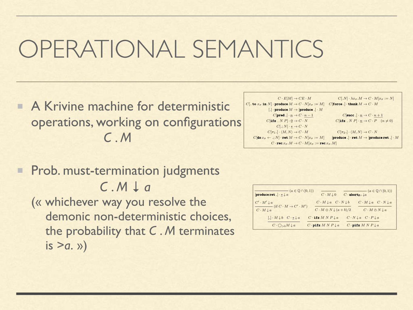
A Krivine machine for deterministic operations, working on configurations C . M
C · E[M ]! CE ·M C[ N ] · �x� .M ! C ·M [x� := N ]
C[ tototo x� ininin N ] · produceproduceproduceM ! C ·N [x� := M ] C[forceforceforce ] · thunkthunkthunkM ! C ·M[ ] · produceproduceproduceM ! [produceproduceproduce ] ·M
C[predpredpred ] · n! C · n� 1 C[succsuccsucc ] · n! C · n+ 1
C[ifzifzifz N P ] · 0! C ·N C[ifzifzifz N P ] · n! C · P (n 6= 0)
C[ ;N ] · ⇤ ! C ·NC[⇡1 ] · hM,Ni ! C ·M C[⇡2 ] · hM,Ni ! C ·N
C[dododox� ;N ] · retretretM ! C ·N [x� := M ] [produceproduceproduce ] · retretretM ! [produceproduceproduceretretret ] ·MC · recrecrecx� .M ! C ·M [x� := recrecrecx� .M ]
(a 2 Q \ [0, 1))[produceproduceproduceretretret ] · ⇤ # a C ·M # 0
(a 2 Q \ [0, 1))C · abortabortabortFFF⌧ #a
C0 ·M 0 # a(if C ·M ! C0 ·M 0
)
C ·M # a
C ·M # a C ·N # b
C ·M �N # (a+ b)/2
C ·M # a C ·N # a
C ·M ? N # a
[ ] ·M # b C · ⇤ # a
C ·�>bM # a
C · ifzifzifz M N P # a
C · pifzpifzpifz M N P # a
C ·N # a C · P # a
C · pifzpifzpifz M N P # a
Figure 3: Operational semantics
We will freely reuse the notations -�, for the similarly defined notions on the re-lated languages CBPV(D, P)+pifzpifzpifz, CBPV(D, P)+�, and CBPV(D, P)+pifzpifzpifz+�. If there is any need to make the language precise, we will mention it explic-itly.
We end this section with a few elementary lemmata, which will come inhandy later on, and which should help the reader train with the way the oper-ational semantics works.
Lemma 4.5 If C · M # a is derivable and b 2 Q is such that 0 b a,then C · M # b is also derivable, whether in CBPV(D, P), CBPV(D, P) + pifzpifzpifz,CBPV(D, P) +�, or CBPV(D, P) + pifzpifzpifz+�.
Proof. Easy induction on the rules of Figure 3. In the case of a derivation ofthe form C ·M �N # a, where a = (a1 + a2)/2, from C ·M # a1 and C ·N # a2,we write b as (b1 + b2)/2 where b1 and b2 are rational and between 0 and a1,resp. a2. (E.g., we let b1 = min(a1, 2b) and b2 = 2b� b1 = max(2b� a1, 0).) Byinduction hypothesis we can derive C ·M # b1 and C ·N # b2, so we can deriveC ·M �N # (b1 + b2)/2 = b. 2
Lemma 4.6 If C ·M ! C 0·M 0, then Pr(C ·M#) � Pr(C 0
·M 0#).
Proof. Whenever we can derive C 0· M 0
# a, we can derive C · M # a by theleftmost rule of the next-to-last row of Figure 3. 2
13
OPERATIONAL SEMANTICS
A Krivine machine for deterministic operations, working on configurations C . M
Prob. must-termination judgments C . M ↓ a (« whichever way you resolve the demonic non-deterministic choices, the probability that C . M terminates is >a. »)
C · E[M ]! CE ·M C[ N ] · �x� .M ! C ·M [x� := N ]
C[ tototo x� ininin N ] · produceproduceproduceM ! C ·N [x� := M ] C[forceforceforce ] · thunkthunkthunkM ! C ·M[ ] · produceproduceproduceM ! [produceproduceproduce ] ·M
C[predpredpred ] · n! C · n� 1 C[succsuccsucc ] · n! C · n+ 1
C[ifzifzifz N P ] · 0! C ·N C[ifzifzifz N P ] · n! C · P (n 6= 0)
C[ ;N ] · ⇤ ! C ·NC[⇡1 ] · hM,Ni ! C ·M C[⇡2 ] · hM,Ni ! C ·N
C[dododox� ;N ] · retretretM ! C ·N [x� := M ] [produceproduceproduce ] · retretretM ! [produceproduceproduceretretret ] ·MC · recrecrecx� .M ! C ·M [x� := recrecrecx� .M ]
(a 2 Q \ [0, 1))[produceproduceproduceretretret ] · ⇤ # a C ·M # 0
(a 2 Q \ [0, 1))C · abortabortabortFFF⌧ #a
C0 ·M 0 # a(if C ·M ! C0 ·M 0
)
C ·M # a
C ·M # a C ·N # b
C ·M �N # (a+ b)/2
C ·M # a C ·N # a
C ·M ? N # a
[ ] ·M # b C · ⇤ # a
C ·�>bM # a
C · ifzifzifz M N P # a
C · pifzpifzpifz M N P # a
C ·N # a C · P # a
C · pifzpifzpifz M N P # a
Figure 3: Operational semantics
We will freely reuse the notations -�, for the similarly defined notions on the re-lated languages CBPV(D, P)+pifzpifzpifz, CBPV(D, P)+�, and CBPV(D, P)+pifzpifzpifz+�. If there is any need to make the language precise, we will mention it explic-itly.
We end this section with a few elementary lemmata, which will come inhandy later on, and which should help the reader train with the way the oper-ational semantics works.
Lemma 4.5 If C · M # a is derivable and b 2 Q is such that 0 b a,then C · M # b is also derivable, whether in CBPV(D, P), CBPV(D, P) + pifzpifzpifz,CBPV(D, P) +�, or CBPV(D, P) + pifzpifzpifz+�.
Proof. Easy induction on the rules of Figure 3. In the case of a derivation ofthe form C ·M �N # a, where a = (a1 + a2)/2, from C ·M # a1 and C ·N # a2,we write b as (b1 + b2)/2 where b1 and b2 are rational and between 0 and a1,resp. a2. (E.g., we let b1 = min(a1, 2b) and b2 = 2b� b1 = max(2b� a1, 0).) Byinduction hypothesis we can derive C ·M # b1 and C ·N # b2, so we can deriveC ·M �N # (b1 + b2)/2 = b. 2
Lemma 4.6 If C ·M ! C 0·M 0, then Pr(C ·M#) � Pr(C 0
·M 0#).
Proof. Whenever we can derive C 0· M 0
# a, we can derive C · M # a by theleftmost rule of the next-to-last row of Figure 3. 2
13
Let Pr(C . M↓) = sup {a | C . M ↓ a}, Pr(M↓) =Pr([_] . M↓)

ADEQUACY
Prop (adequacy).For every M : FVunit, — ⟦M⟧=⊥ and Pr(M↓)=0, or — ⟦M⟧=∅ and Pr(M↓)=1, or else — Pr(M↓)=min {ν({⊤}) | ν ∈ ⟦M⟧}
Jx�K ⇢ = ⇢(x�)
J�x�.MK ⇢ = V 2 J�K 7! JMK (⇢[x� 7! V ]) JMNK ⇢ = JMK ⇢(JNK ⇢)JproduceproduceproduceMK ⇢ = ⌘Q(JMK ⇢)
JM tototo x� ininin NK ⇢ = (V 2 J�K 7! JNK ⇢[x� 7! V ])⇤(JMK ⇢)JthunkthunkthunkMK ⇢ = JMK ⇢ JforceforceforceMK ⇢ = JMK ⇢
J⇤K ⇢ = > JnK ⇢ = n
JsuccsuccsuccMK ⇢ =
⇢n+ 1 if n = JMK ⇢ 6= ?? otherwise
JpredpredpredMK ⇢ =
⇢n� 1 if n = JMK ⇢ 6= ?? otherwise
Jifzifzifz M N P K ⇢ =
8<
:
JNK ⇢ if JMK ⇢ = 0JP K ⇢ if JMK ⇢ 6= 0,?? if JMK ⇢ = ?
JM ;NK ⇢ =
⇢JNK ⇢ if JMK ⇢ = >? otherwise
J⇡1MK ⇢ = m, J⇡2MK ⇢ = n where JMK ⇢ = (m,n)
JhM,NiK ⇢ = (JMK ⇢, JNK ⇢)JretretretMK ⇢ = �JMK⇢
Jdododox� M ;NK ⇢ = (V 2 J�K 7! JNK ⇢[x� 7! V ])†(JMK ⇢)
JM �NK ⇢ =1
2(JMK ⇢+ JNK ⇢)
JM ? NK ⇢ = JMK ⇢ ^ JNK ⇢ JabortabortabortFFF⌧ K ⇢ = ;
Jrecrecrecx�.MK ⇢ = lfp(V 2 J�K 7! JMK ⇢[x� 7! V ])
Jpifzpifzpifz M N P K ⇢ =
8<
:
JNK ⇢ if JMK ⇢ = 0JP K ⇢ if JMK ⇢ 6= 0,?JNK ⇢ ^ JP K ⇢ if JMK ⇢ = ?
J�>bMK ⇢ =
8<
:
> if JMK ⇢ 6= ? andb⌧ ⌫({>}) for every ⌫ 2 JMK ⇢
? otherwise
Figure 2: Denotational semantics
10

ADEQUACY
Prop (adequacy).For every M : FVunit, — ⟦M⟧=⊥ and Pr(M↓)=0, or — ⟦M⟧=∅ and Pr(M↓)=1, or else — Pr(M↓)=min {ν({⊤}) | ν ∈ ⟦M⟧}
I.e., Pr(M↓)=h*(⟦M⟧) where h(ν) = ν({⊤})
Proof: by suitable logical relations.
Jx�K ⇢ = ⇢(x�)
J�x�.MK ⇢ = V 2 J�K 7! JMK (⇢[x� 7! V ]) JMNK ⇢ = JMK ⇢(JNK ⇢)JproduceproduceproduceMK ⇢ = ⌘Q(JMK ⇢)
JM tototo x� ininin NK ⇢ = (V 2 J�K 7! JNK ⇢[x� 7! V ])⇤(JMK ⇢)JthunkthunkthunkMK ⇢ = JMK ⇢ JforceforceforceMK ⇢ = JMK ⇢
J⇤K ⇢ = > JnK ⇢ = n
JsuccsuccsuccMK ⇢ =
⇢n+ 1 if n = JMK ⇢ 6= ?? otherwise
JpredpredpredMK ⇢ =
⇢n� 1 if n = JMK ⇢ 6= ?? otherwise
Jifzifzifz M N P K ⇢ =
8<
:
JNK ⇢ if JMK ⇢ = 0JP K ⇢ if JMK ⇢ 6= 0,?? if JMK ⇢ = ?
JM ;NK ⇢ =
⇢JNK ⇢ if JMK ⇢ = >? otherwise
J⇡1MK ⇢ = m, J⇡2MK ⇢ = n where JMK ⇢ = (m,n)
JhM,NiK ⇢ = (JMK ⇢, JNK ⇢)JretretretMK ⇢ = �JMK⇢
Jdododox� M ;NK ⇢ = (V 2 J�K 7! JNK ⇢[x� 7! V ])†(JMK ⇢)
JM �NK ⇢ =1
2(JMK ⇢+ JNK ⇢)
JM ? NK ⇢ = JMK ⇢ ^ JNK ⇢ JabortabortabortFFF⌧ K ⇢ = ;
Jrecrecrecx�.MK ⇢ = lfp(V 2 J�K 7! JMK ⇢[x� 7! V ])
Jpifzpifzpifz M N P K ⇢ =
8<
:
JNK ⇢ if JMK ⇢ = 0JP K ⇢ if JMK ⇢ 6= 0,?JNK ⇢ ^ JP K ⇢ if JMK ⇢ = ?
J�>bMK ⇢ =
8<
:
> if JMK ⇢ 6= ? andb⌧ ⌫({>}) for every ⌫ 2 JMK ⇢
? otherwise
Figure 2: Denotational semantics
10

NOTE
None of that yet requires CCCs ofcontinuous (or algebraic) domains

NOTE
None of that yet requires CCCs ofcontinuous (or algebraic) domains
Soundness/adequacy workseven for non-call-by-push-value probabilistic languages, working in the CCC Dcpo
dcpos

NOTE
None of that yet requires CCCs ofcontinuous (or algebraic) domains
Soundness/adequacy workseven for non-call-by-push-value probabilistic languages, working in the CCC Dcpo
Continuity is only needed for more advanced applications: — full abstraction (next) — commutativity of the V monad (Fubini) at higher types
dcpos
THE CONTEXTUAL PREORDER
Let M ⪯ N iff for every context C of output type FVunit, Pr(C . M↓) ≤ Pr(C . N↓)

THE CONTEXTUAL PREORDER
Let M ⪯ N iff for every context C of output type FVunit, Pr(C . M↓) ≤ Pr(C . N↓)
M ⪯ N iff for every context C of output type FVunit, h*(⟦C[M]⟧) ≤ h*(⟦C[N]⟧) (adequacy)

THE CONTEXTUAL PREORDER
Let M ⪯ N iff for every context C of output type FVunit, Pr(C . M↓) ≤ Pr(C . N↓)
M ⪯ N iff for every context C of output type FVunit, h*(⟦C[M]⟧) ≤ h*(⟦C[N]⟧) (adequacy)
Corollary. If ⟦M⟧ ≤ ⟦N⟧ then M ⪯ N.

THE CONTEXTUAL PREORDER
Let M ⪯ N iff for every context C of output type FVunit, Pr(C . M↓) ≤ Pr(C . N↓)
M ⪯ N iff for every context C of output type FVunit, h*(⟦C[M]⟧) ≤ h*(⟦C[N]⟧) (adequacy)
Corollary. If ⟦M⟧ ≤ ⟦N⟧ then M ⪯ N.
Proof. ⟦C[M]⟧ = ⟦C⟧ (⟦M⟧) ≤ ⟦C⟧ (⟦N⟧) = ⟦C[N]⟧ since ⟦C⟧ (= ⟦λx . C[x]⟧) is Scott-continuous hence monotonic. Then apply h*, which is monotonic as well. ☐

FULL ABSTRACTION?
Conjecture (full abstraction): ⟦M⟧ ≤ ⟦N⟧ iff M ⪯ N.

FULL ABSTRACTION?
Conjecture (full abstraction): ⟦M⟧ ≤ ⟦N⟧ iff M ⪯ N.
Wrong. — missing parallel if (pifz), as in (Plotkin77) — even with pifz, missing statistical termination testers ⃝ >b, as in (GL15): ⃝ >b M terminates if M terminates with prob. >b, otherwise does not terminate.

FULL ABSTRACTION
Adding pifz + ⃝ >b,
Theorem (full abstraction): with pifz and ⃝ >b, ⟦M⟧ ≤ ⟦N⟧ iff M ⪯ N.
For the argument, see the paper. Uses the deep structure of continuous coherent dcpos and continuous complete lattices. Core: theorems on (effective) coincidence of topologies.

SUMMARY
Circumventing the trouble with Vby using two classes of types, as provided by call-by-push-value
We obtain (inequational) full abstraction with prob. choice + demonic non-determinism
Questions?