A probabilistic calibration of climate sensitivityand terrestrial carbon change in GENIE-1

Philip B. Holden Æ N. R. Edwards Æ K. I. C. Oliver ÆT. M. Lenton Æ R. D. Wilkinson

Received: 4 February 2009 / Accepted: 7 July 2009

� Springer-Verlag 2009

Abstract In order to investigate Last Glacial Maximum

and future climate, we ‘‘precalibrate’’ the intermediate

complexity model GENIE-1 by applying a rejection sam-

pling approach to deterministic emulations of the model.

We develop *1,000 parameter sets which reproduce the

main features of modern climate, but not precise observa-

tions. This allows a wide range of large-scale feedback

response strengths which generally encompass the range

of GCM behaviour. We build a deterministic emulator

of climate sensitivity and quantify the contributions of

atmospheric (±0.93�C, 1r) vegetation (±0.32�C), ocean

(±0.24�C) and sea–ice (±0.14�C) parameterisations to the

total uncertainty. We then perform an LGM-constrained

Bayesian calibration, incorporating data-driven priors and

formally accounting for structural error. We estimate cli-

mate sensitivity as likely (66% confidence) to lie in the

range 2.6–4.4�C, with a peak probability at 3.6�C. We

estimate LGM cooling likely to lie in the range 5.3–7.5�C,

with a peak probability at 6.2�C. In addition to estimates of

global temperature change, we apply our ensembles to

derive LGM and 2xCO2 probability distributions for land

carbon storage, Atlantic overturning and sea–ice coverage.

Notably, under 2xCO2 we calculate a probability of 37%

that equilibrium terrestrial carbon storage is reduced from

modern values, so the land sink has become a net source of

atmospheric CO2.

Keywords Climate sensitivity � Last glacial maximum �Precalibration � Structural error � Emulation � GENIE-1

1 Introduction

Climate sensitivity DT2x, defined as the equilibrium global-

mean temperature response to a doubling of atmospheric

CO2, provides the conventional measure of the change of

the climate in response to increasing greenhouse gas con-

centrations. The best current estimate of DT2x is that it is

likely (66% confidence) to lie in the region 2.0–4.5�C

(IPCC 2007), a figure which famously has changed little

since Arrhenius (1896) derived the first estimate of *5�C.

The quantification of DT2x is approached through perturbed

physics ensembles (e.g. Stainforth et al. 2005), multi-

model ensembles (e.g. Webb et al. 2006), or by con-

straining possible future changes with respect to known

past changes (e.g. Lea 2004; Annan and Hargreaves 2006).

Data and models can be combined through an observa-

tionally constrained perturbed physics experiment (e.g.

Knutti et al. 2002; Schneider von Deimling et al. 2006a);

the combined approach has the advantage that whilst

incorporating knowledge of previous climate states it does

not assume perfect symmetry between non-analogue states,

as estimates based exclusively on observational data are

required to do. Here, we attempt to build upon Schneider

von Deimling et al. (2006a), who derived a perturbed-

physics estimate of DT2x using an interval approach to

P. B. Holden (&) � N. R. Edwards � K. I. C. Oliver

Department of Earth and Environmental Sciences,

The Open University, Milton Keynes MK7 6AA, UK

e-mail: p.b.holden@open.ac.uk

T. M. Lenton

School of Environmental Sciences, University of East Anglia,

Norwich NR4 7TJ, UK

T. M. Lenton

Tyndall Centre for Climate Change Research, Norwich, UK

R. D. Wilkinson

Department of Probability and Statistics, University of Sheffield,

Sheffield S3 7RH, UK

123

Clim Dyn

DOI 10.1007/s00382-009-0630-8

constrain CLIMBER-2 with last glacial maximum (LGM)

tropical Atlantic sea surface temperature (SST). While this

approach provided an estimate for DT2x very likely (90%

confidence) in the range 1.2–4.3�C, the upper limit was

increased to *5.4�C when poorly quantified uncertainties,

in particular relating to model structural error, were

incorporated. Although the extent to which changes at the

LGM can constrain future climate is limited by an

incomplete understanding of relevant processes (Crucifix

2006), the LGM is relatively well understood, both in terms

of forcing and climate, and provides an ideal model vali-

dation state, provided the uncertainties arising from model

structural error are properly addressed.

We apply the model GENIE-1 (Lenton et al. 2006), an

intermediate complexity model built around a 3D ocean

model, incorporating dynamic vegetation and sea–ice

modules and coupled to an Energy Moisture Balance

Model of the atmosphere. Our study complements

Schneider von Deimling et al. (2006a), who applied

CLIMBER-2, incorporating a 2.5D dynamical-statistical

atmosphere coupled to a zonally averaged ocean model and

fixed vegetation. Our approach does not represent an

attempt to reduce uncertainty in DT2x—an unrealistic

objective in view of the greatly simplified atmospheric

model and outgoing longwave radiation (OLR) feedback

parameterisation—but is rather an attempt to investigate

the contribution of different components of the Earth sys-

tem to uncertainty in DT2x. The use of the simplified

atmosphere of GENIE-1 has the advantage that robust

statistical techniques can be applied as a consequence of

high computational efficiency (*3,000 model years per

CPU hour in the configuration we apply here). Although

much work has been done elsewhere investigating atmo-

spheric uncertainties, in particular relating to the parame-

terisation of clouds (e.g. Webb et al. 2006), other

uncertainties, in particular those arising from vegetation,

have received less attention. We note that even in cases

where these processes play a minor role in DT2x per se, they

nevertheless represent responses to climate change which

are important in their own right.

Our approach is designed to allow for the uncertainty

arising from structural error es, the irreducible error that

remains when the ‘‘best’’ parameter inputs are applied to a

model (Rougier 2007), as distinct from the parametric error

ep that results from a non-optimal choice of parameter

inputs and which can be reduced by more careful tuning.

The quantification of es is a highly demanding task,

requiring the anticipation of the consequences of missing

and/or poorly understood process and their complex

interactions; Murphy et al. (2007) describe an approach in

which multi-model ensembles are used to derive a lower

bound for es under the assumption that inter-model vari-

ances are likely to reflect structural error. Such an approach

cannot account for structural deficiencies which are com-

mon to all models. Here we apply the concept of ‘‘pre-

calibration’’ (Rougier et al. in preparation), whereby the

model is required only to produce a ‘‘plausible’’ climate

state, reproducing the main features of the climate system

but not constrained by detailed observations. The approach

is an attempt to enable progress without a precise quanti-

fication of structural error; by applying only very weak

constraints to the 26 input parameters which we allow to

vary, and also to the modelled modern climate state we

accept as plausible, we allow a wide range of large-scale

feedback response strengths which generally encompass

the range of behaviour exhibited by high resolution multi-

member ensembles (c.f. Murphy et al. 2007). We do not

attempt to minimise parametric error (as would be the case

in a conventional calibration) but rather deliberately allow

it to dominate model uncertainty in an attempt to bypass

the need for a quantification of structural error.

Computational and time constraints mean that it is

not feasible to explore the entire 26 dimensional input

parameter space with a naı̈ve Monte Carlo approach.

Instead, we build a computationally cheap surrogate for

GENIE-1 called an emulator (Santner et al. 2003) using an

ensemble of 1,000 GENIE-1 model runs (described in

Sect. 3). Only ten of these ensemble members produced

modern plausible climates (as defined above), largely as a

consequence of the weak constraints imposed on parameter

ranges and the corresponding sparse coverage of input

space. We then apply a rejection sampling method known

as approximate bayesian computation (ABC) (Beaumont

et al. 2002) to find a collection of 1,000 parameter vectors

that the emulator predicts will be modern plausible. These

emulator-filtered parameterisations are then validated by

performing a second modern ensemble with GENIE-1,

checking that each parameter vector does indeed lead to a

plausible modern climate state. Two further ensembles

with LGM and doubled CO2 boundary conditions are then

generated, using the filtered input vectors, in order to

investigate a range of Earth system responses (temperature

and vegetation distributions, Atlantic overturning and sea–

ice coverage). We discuss the range of model responses in

Sect. 4.

In order to examine parameter interactions in setting

climate sensitivity, in Sect. 5 we represent DT2x through a

further emulation. We use the emulator to perform a

‘‘global sensitivity analysis’’ (Saltelli et al. 2000), appor-

tioning variance in the output to uncertainty in the input

parameters, thus providing quantification of the relative

contributions of various parameterisations to the overall

uncertainty in DT2x.

To derive a probabilistic estimate for DT2x we apply

Rougier (2007) to the GENIE-1 ensemble output. The

analytical approach, described in Sect. 6, ascribes

P. B. Holden et al.: A probabilistic calibration of climate sensitivity

123

probability weightings to the parameter vectors, con-

strained by observational estimates of LGM tropical SST,

accounting for the uncertainty arising from structural error

and incorporating prior knowledge about parameters where

applicable. This enables us to derive calibrated probabi-

listic statements about the whole Earth System response in

GENIE-1, including changes in land carbon storage, in

both LGM and 2xCO2 states. The calculation of climate

sensitivity and sensitivity analysis is described in Sect. 7.

The application to other Earth System responses is

described in Sect. 8.

2 GENIE-1

We apply the intermediate complexity model GENIE-1, at

a resolution of 36 9 36 9 8, in the configuration described

by Lenton et al. (2006). The physical model comprises

C-GOLDSTEIN, a 3D frictional geostrophic ocean with

eddy-induced and isopycnal mixing coupled to a 2D fixed

wind-field energy-moisture balance atmosphere and a

dynamic and thermodynamic sea–ice component (Edwards

and Marsh 2005). The physical model is coupled to ENTS,

a minimum spatial model of vegetation carbon, soil carbon

and soil water storage (Williamson et al. 2006). LGM

Boundary conditions are as described in Lunt et al. (2006),

applying the ICE-4G LGM ice-sheet Peltier (1994) and

Berger (1978) orbital parameters and an atmospheric CO2

concentration of 190 ppm. Although LGM dust forcing is

neglected in the simulations, this bias is accounted for in

the probabilistic analysis (Sects. 6 and 7). All simulations

are run to equilibrium over 5,000 years.

Two changes from Lenton et al. (2006) are incorporated:

(1) In order to provide realistic land temperatures for

vegetation and snow cover, the effect of orography,

neglected in Lenton et al. (2006), is applied to surface

processes by applying a constant lapse rate of

6.5 9 10-3�C m-1. An adjustment for surface oro-

graphy is not applied to atmospheric processes as

these represent averages throughout the depth of the

1-layer atmosphere.

(2) We assume a simple term for outgoing longwave

radiation (OLR), an assumption which is discussed in

some detail in Sect. 6. OLR at each grid cell is given

by:

L�out ¼ LoutðT; qÞ � KLW0 � KLW1DT ð1Þ

where Lout(T, q) is the unmodified ‘‘clear-skies’’ OLR

term of Thompson and Warren (1982). KLW0, inclu-

ded to allow for uncertainty in the modern state, was

allowed to vary in the range 5 ± 5 Wm-2, a range

which an initial exploratory ensemble suggested was

sufficiently broad to cover plausible modern output

space. Positive values for KLW0 are assumed as the

term represents a perturbation to the clear skies

expression; neglecting this term lead to an underes-

timation of modern air temperatures by *2–3�C in

three tuned parameterisations of the model (Lenton

et al. 2006). KLW1DT (Matthews and Caldeira 2007)

is primarily designed to capture unmodelled cloud

response to global average temperature change DT.

The effect of this simple term for OLR, in combi-

nation with a dynamically simple atmosphere, is that

all of the resulting structural error must be accounted

for by uncertainty in the value for KLW1 which would

in practice not be constant. KLW1 was allowed to vary

from -0.5 to 0.5 W m-2 K-1, values suggested by

an exploratory ensemble, as realistic LGM climates

cannot be produced with values outside of this range.

This range of KLW1 values suggests that the dominant

processes represented by this parameter in GENIE-1

are uncertainties in cloud and lapse rate feedbacks,

which approximately cancel in AOGCMs (at least in

the ensemble mean) and are estimated at 0.69 ±

0.38 W m-2 K-1 and -0.84 ± 0.26 W m-2 K-1

respectively (Soden and Held 2006). We note that

this cancellation may to some extent break down

when latitudinal variations are considered (Colman

and McAvaney 2009), so the assumption of a glob-

ally constant OLR correction will inevitably under-

estimate regional uncertainty. Uncertainty in water

vapour feedbacks is captured through the relative

humidity threshold for precipitation, a parameter

which is varied in this study, and through variability

in the clear skies expression, via the uncertainty in

temperature and humidity fields; in general the rela-

tionship between individual parameterisations and

specific feedback strengths is not simple.

3 Precalibration of GENIE-1

Here we apply the concept of precalibration (Rougier et al.

in preparation) in order to develop a *1,000 member

parameter set to apply as input to three ensembles (with

modern, LGM and 2xCO2 boundary conditions). This

approach, summarised in a flow chart in Fig. 1, attempts to

progress without a quantification of structural error by

ruling out very bad parameter choices, but making little

attempt to identify good candidates. To achieve this, we not

only apply weak prior constraints to the parameters

(through uniform, broad input parameter ranges) but also to

the range of model output we are prepared to accept as

valid; we require our model to reproduce the main features

P. B. Holden et al.: A probabilistic calibration of climate sensitivity

123

of the climate system but do not require it to accurately

reproduce observations. By generating a wide spread of

climate states, we assert that parametric error dominates

over structural error so that we can capture the modelled

uncertainty without explicitly quantifying the structural

error. Analogously to Murphy et al. (2007), a minimum

requirement is that we can demonstrate that our ensemble

encompasses the range of behaviour displayed in multi-

model ensembles, a question we address in Sect. 4.

Twenty-six parameters were varied over the wide ranges

given in Table 1. Parameter ranges were derived from the

references supplied in Table 1, with minor adjustments

made on the basis of an initial exploratory ensemble not

described here. We define h to be the 26-dimensional input

parameter vector, and generate a 1,000 member maximin

Latin hypercube:

D ¼ fh ji ; j ¼ 1; . . .; 1000; i ¼ 1; . . .; 26g ð2Þ

where the subscript i represents the 26 parameters and the

superscript j represents the 1,000 different realisations

(parameter vectors). The 26th parameter FFX does not play

a role in the equilibrium calculations described here but

was retained in the statistical analysis as a check for over-

fitting.

The parameter set D was applied as input to an initial

modern ensemble of GENIE-1. The purpose of this initial

ensemble is to provide the data required to build five emu-

lators of modern climate. These emulators are computa-

tionally cheap (polynomial) relationships between the 26

input parameters and the five selected model output

diagnostics. The output diagnostics are designed to test the

ocean (Atlantic overturning strength), atmosphere (global

average Surface Air Temperature, SAT), sea–ice (annual

average Antarctic sea–ice area) and land carbon storage

(total vegetative carbon and total soil carbon). We subse-

quently apply these emulators to design the parameter set

applied to the ensembles described in subsequent sections.

Before building the emulators, the five modern plausi-

bility tests were applied to the output of the GENIE-1

ensemble. The required ranges are summarised in Table 2

(‘‘plausibility test Rk’’). These ranges are substantially

broadened from observational uncertainty in order to allow

for model structural error and ensure that the range of

plausible model outcomes contains the ‘‘true’’ climate

state. The ranges selected for precalibration filtering are

model dependent (Rougier et al. in preparation) as, for

instance, low resolution model outcomes would be tend

to be viewed more leniently. We define f(h) to be the

5-dimensional summary (the plausibility characteristics) of

GENIE-1 run at h. A parameter vector was considered

modern plausible only if all five of the plausibility metrics

fell within the accepted ranges:

jfkðh jÞ � lkj � ek for k ¼ 1; . . .; 5 ð3Þ

where lk are the mid points and ek the half widths of the

plausibility ranges Rk in Table 2. In this initial ensemble

only ten of the simulations were found to provide a plau-

sible modern climate state for all five constraints simulta-

neously, reflecting the broad parameter ranges supplied and

consequent under-sampling of input space.

Modern plausibility tests (Eq. 3)

Emulate GENIE-1 output

1,000 member GENIE-1 ensemble “P”; emulator-

plausible parameterisations

10 plausible ensemble members

Rejection sampling of emulator output (Eq. 5)

Modern plausibility tests (Eq. 3) & no “runaway”LGM

cooling

480 plausible members = LPC parameter set

Plausible LGM Antarctic anomaly?

1,000 member GENIE-1 ensemble “D”; Maximin Latin Hypercube with broad, uniform distributions for 26 parameters

Five plausibility emulators (Atlantic overturning, global

SAT, Antarctic sea ice, vegetative & soil carbon

894 plausible members = MPC parameter set

Figure 2Calculate Total Effect (Eq. 4)

Emulate GENIE-1 output

1,000 member GENIE-1 ensemble “D”; Maximin Latin Hypercube with broad, uniform distributions for 26 parameters

Five plausibility emulators (Atlantic overturning, global

SAT, Antarctic sea ice, vegetative & soil carbon

894 plausible members = MPC parameter set

Fig. 1 Flow chart of the

precalibration approach

(Sect. 3) used to construct the

MPC and LPC parameter sets

P. B. Holden et al.: A probabilistic calibration of climate sensitivity

123

In order to produce a large plausibility-constrained

parameter set, deterministic emulators fk were built for

each of the five metrics, following Rougier et al. (in

preparation), performing stepwise logistic regression,

including linear, quadratic and cross terms for all 26

variables. (The DT2x emulator, described in Sect. 5, addi-

tionally includes cubic terms, thus allowing three-way

interactions). Prior to fitting, variables were linearly map-

ped onto the range [-1, 1] so that odd and even functions

are orthogonal, improving the selection of terms. Stepwise

selection was performed using the stepAIC function

(Venables and Ripley 2002) in R (R Development Core

Team 2004), minimising the Akaike Information Criterion

(which attempts to best explain the data with the minimum

Table 1 Ensemble parameters:

25 parameters were varied

across the ranges detailed below

The parameters were

incorporated into a uniformly

spaced maximin Latin

Hypercube for the initial

ensemble (used to derive

plausibility emulators) and

retained as input bounds for the

ABC-filtering process which

derived the plausibility

parameter set. References for

the parameters can be found in

(a) Edwards and Marsh (2005),

(b) Lenton et al. (2006), (c)

Thompson and Warren (1982),

(d) Matthews and Caldeira

(2007), (e) Williamson et al.

(2006), (f) Wullshleger et al.

(1995) and (g) Lenton and

Huntingford (2003)

Parameter description Ref Minimum Maximum

OHD, Ocean isopycnal diffusivity (m2 s-1) a 300 9,000

OVD, Ocean diapycnal diffusivity (m2 s-1) a 2 9 10-6 2 9 10-4

ODC, Ocean friction coefficient (days-1) a 0.5 5.0

WSF, Wind scale coefficient a 1 3

SID, Sea ice diffusivity (m2 s-1) a 300 25,000

SIA, Sea ice albedo 0.5 0.7

AHD, Atmospheric heat diffusivity (m2 s-1) a 1 9 106 5 9 106

WAH, Width of atmospheric heat diffusivity (Radians) a 0.5 2.0

SAD, Slope of atmospheric diffusivity a 0 0.25

AMD, Atmospheric moisture diffusivity (m2 s-1) a 5 9 104 5 9 106

ZHA, Heat advection factor a 0 1

ZMA, Moisture advection factor a 0 1

APM, Atlantic–Pacific freshwater flux (Sv) a 0.05 0.64

RMX, Relative humidity threshold for precipitation b 0.6 0.9

OL0, KLW0 clear skies OLR reduction (W m-2) c 0 10

OL1, KLW1 OLR feedback (W m-2 K-1) d -0.5 0.5

VPC (k14), photosynthesis half-saturation to CO2 (ppmv) e, f 0 700

VFC (k17), fractional vegetation dependence on Cveg (kgC-1 m2) e 0.2 1.0

VBP (k18), base rate of photosynthesis (kgC m-2 year-1) e 3.0 5.5

VRA (k20), vegetation respiration activation energy (J mol-1) e, g 24,000 72,000

VRR (k24), vegetation respiration rate (year-1) e 0.16 0.3

LLR (k26), leaf litter rate (year-1) e 0.075 0.260

SRR (k29) soil respiration rate (year-1) e 0.1 0.3

SRT (k32), soil respiration activation temperature (K) e, g 197 241

KZ0, roughness dependence on Cveg (m-3 kgC) e 0.02 0.08

FFX, dummy variable N/A N/A

Table 2 The 5 plausibility metrics

Plausibility

test Rk

ABC test Rk* MPC ensemble mean

and 1r deviation

MPC ensemble

range

Ocean Atlantic overturning stream function (Sv) 10–30 13–19 18 ± 3 10–29

EMBM Global SAT (�C) 12–16 13.5–15.5 14.1 ± 0.7 12–16

Sea ice Antarctic Sea–ice area (million km2) 3–20 8–12 9 ± 3 3–19

Vegetation Total carbon (GTC) 300–700 350–550 440 ± 60 300–610

Soil Total carbon (GTC) 750–2,000 1,100–1,500 1,250 ± 170 840–1,880

The Plausibility test Rk describes the range of values which are accepted as ‘‘plausible’’ realisations of GENIE-1. The ABC test Rk* describes the

range of values which are accepted as potentially plausible realisations of the emulators: parameter sets found to satisfy all 5 ABC criteria (Eq. 5)

were supplied as input to GENIE-1 and accepted as plausible if GENIE-1 output satisfied all 5 plausibility criteria (Eq. 3). The averages, standard

deviations and ranges of the GENIE output from the 894 MPC parameter sets are provided in the third and fourth columns

P. B. Holden et al.: A probabilistic calibration of climate sensitivity

123

of free parameters). Terms were subsequently removed by

applying the more stringent Bayes Information Criterion

(which penalises free parameters more strongly). Three of

our chosen 26 parameters can have no role in the modern

state: OL1 (KLW1 in Eq. 1), VPC (describing the CO2

fertilisation of photosynthesis and normalised to a modern

response at 280 ppm) and the dummy variable FFX; the

final models were pruned by selecting a significance

threshold sufficient to eliminate these three parameters

from the emulators and minimise overfitting.

In order to investigate the role of individual parameters

in determining a plausible modern state, a global sensitivity

analysis (Saltelli et al. 2000) was performed for each

emulator, calculating the contribution of each parameter to

the variance of that emulator. For each of the emulators fk,

we calculate the total effect VkT of hi. This represents the

remaining uncertainty in fk(h) after we have learnt every-

thing except hi i.e. the expected variance of fk(h) | h[-i],

where h[-i] = (h1,…,hi-1, hi?1,…, hn):

VkTi¼ E½�i�Varhi

ðfkðhÞjh �i½ �Þ

¼ZZðfkðhÞ � EðfkðhÞjh½�i�ÞÞ2dhidh½�i� ð4Þ

which is readily solved analytically for the polynomial

emulators and uniform prior distributions considered in this

section.

Figure 2 plots the total effect of each parameter

(normalised to a total of 100%) for each of the emulators,

thus illustrating the relative importance of each parameter

in controlling the five plausibility metrics. The emulators

exhibit an R2 of 98% (SAT), 88% (Atlantic overturning),

91% (Antarctic sea ice area), 98% (vegetative carbon)

and 94% (soil carbon) with respect to the simulated

output, and thus provide a reasonably accurate description

of the apportionment of variance of GENIE-1. It is

important to note that the total effect depends upon the

range across which the parameter is allowed to vary, and

consequentially it is a subjective measure, dependent

upon the expert judgement applied in determining these

ranges.

(1) Uncertainties in global average SAT are dominated

by uncertainties in OL0 (primarily the effect of cloud

uncertainty on the modern-day radiation balance),

RMX, the relative humidity threshold for precipita-

tion (through its influence on the water vapour

feedback), AHD, the atmospheric heat diffusivity,

and VFC, defining the dependence of fractional

vegetation coverage on vegetation carbon though its

control on land surface albedo.

(2) In GENIE-1, uncertainties in Atlantic overturning

are dominated by the atmospheric transport of

freshwater through APM, the Atlantic-Pacific fresh-

water flux adjustment (which corrects for the

*0.29 Sv underestimation of atmospheric moisture

transport from the Atlantic to the Pacific and is

required for a stable Atlantic overturning, Edwards

and Marsh 2005) and AMD, the atmospheric mois-

ture diffusivity. Ocean tracer diffusivities (OHD and

OVD) and the ocean drag coefficient (ODC) also

play a significant role.

(3) Uncertainties in sea–ice, though substantial, are not

dominated (in GENIE-1) by the sea–ice parameteri-

sations themselves, but rather by the parameterisa-

tions of atmospheric and ocean transport, and exhibit

a close coupling with parameters that control global

average temperature and the equator-pole temperature

gradient.

0%

10%

20%

30%

40%

50%

60%

70%

80%

OV

D

OD

C

OH

D

WS

F

SIA

SID

OL0

RM

X

AH

D

AM

D

AP

M

WA

H

SA

D

ZM

A

ZH

A

VF

C

LLR

VB

P

SR

T

SR

R

VR

A

KZ

0

VR

R

To

tal E

ffec

t (n

orm

alis

ed t

o 1

00%

)

Air Temp Overturning Sea Ice Vegetation Soil

Fig. 2 The relative role of

parameters in determining the

modern state. The total effect of

each parameter (the expectation

of the variance which remains

when all other parameters are

known) is calculated for each

emulator. These are normalised

to 100% to approximate the

percentage contribution of each

parameter to the variance of

each emulator as an illustration

of which parameters drive

uncertainty in the modern state

P. B. Holden et al.: A probabilistic calibration of climate sensitivity

123

(4) Although uncertainties in vegetation are largely

controlled by parameters which exert control on the

rate of photosynthesis (notably VBP, the base rate of

photosynthesis, and VFC) and the leaf litter rate

(LLR), atmospheric transport through heat diffusivity

(AHD) and moisture diffusivity (AMD) also play an

important role.

(5) Uncertainty in soil carbon is dominated by the

parameterisation of soil respiration through SRT,

the activation temperature for soil respiration, and

SRR, the soil respiration rate, although the parameters

which control the source of soil carbon, through the

production of vegetation carbon and ultimately leaf

litter, play a significant role.

We used these emulators as a cheap surrogate for

GENIE-1 in order to perform the precalibration. An

approximate bayesian computation (ABC) method (Beau-

mont et al. 2002) was applied to the emulators. This

procedure updates the uniform prior distribution for h

-180 -90 0 90 180-90

-45

0

45

90

Longitude [°E]

Latit

ude

[ °N]

Modern Average SAT

-40 -30 -20 -10 0 10 20 30 40

-180 -90 0 90 180-90

-45

0

45

90

Longitude [°E]

Latit

ude

[ °N]

Modern SAT Standard Deviation

0 1 2 3 4 5 6 7 8 9 10

-180 -90 0 90 180-90

-45

0

45

90

Longitude [°E]

Latit

ude

[ °N]

LGM Average SAT Anomaly

-15 -10 -5 0 5 10 15

-180 -90 0 90 180-90

-45

0

45

90

Longitude [°E]

Latit

ude

[ °N]

LGM Standard Deviation of SAT Anomaly

0 0.5 1 1.5 2 2.5 3 3.5 4

-180 -90 0 90 180-90

-45

0

45

90

Longitude [°E]

Latit

ude

[ °N]

2xCO2 Standard Deviation of SAT Anomaly

0 0.5 1 1.5 2 2.5

-180 -90 0 90 180-90

-45

0

45

90

Longitude [°E]

Latit

ude

[ °N]

2xCO2 Average SAT Anomaly

-10 -8 -6 -4 -2 0 2 4 6 8 10

-180 -90 0 90 180-90

-45

0

45

90

Longitude [°E]

Latit

ude

[ °N]

-40 -30 -20 -10 0 10 20 30 40

-180 -90 0 90 180-90

-45

0

45

90

Longitude [°E]

Latit

ude

[ °N]

0 1 2 3 4 5 6 7 8 9 10

-180 -90 0 90 180-90

-45

0

45

90

Longitude [°E]

Latit

ude

[ °N]

-15 -10 -5 0 5 10 15

-180 -90 0 90 180-90

-45

0

45

90

Longitude [°E]

Latit

ude

[ °N]

0 0.5 1 1.5 2 2.5 3 3.5 4

-180 -90 0 90 180-90

-45

0

45

90

Longitude [°E]

Latit

ude

[ °N]

0 0.5 1 1.5 2 2.5

-180 -90 0 90 180-90

-45

0

45

90

Longitude [°E]

Latit

ude

[ °N]

-10 -8 -6 -4 -2 0 2 4 6 8 10

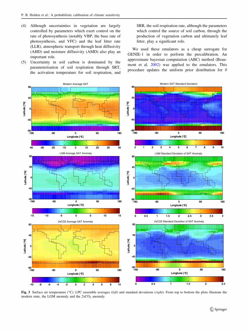
Fig. 3 Surface air temperature (�C). LPC ensemble averages (left) and standard deviations (right). From top to bottom the plots illustrate the

modern state, the LGM anomaly and the 2xCO2 anomaly

P. B. Holden et al.: A probabilistic calibration of climate sensitivity

123

(Table 1) in light of the emulated plausibility metrics fk(h)

to find a posterior distribution for h. This is accomplished

by drawing parameters randomly from their defined input

ranges and accepting them as potentially valid if the

emulators reproduce observations to within an acceptable

level on each of the plausibility measures:

jfkðhÞ � l�k j � e�k ð5Þ

where lk* are the mid points and ek

* the half widths of the

ABC ranges Rk* in Table 2. For the purposes of ABC fil-

tering, accepted ranges were narrowed from the plausibility

ranges Rk. This is partly to avoid unnecessary wastage

caused by imperfect emulation of the model and partly,

given emulator error, to ensure the ensemble average out-

put is centred close to observations, in order to minimise

potential bias in the modern state (on the assumption that

our expectation of structural error has zero mean). This

process was continued until we had accepted 1,000 values

of h. The resulting set is labelled P. This required sampling

*12 million randomly generated values of h, illustrating

the necessity for emulation (or alternatively a very much

more efficient sampling procedure). We note that although

we describe this process as a precalibration, rather than a

calibration, this distinction simply reflects the broad ranges

we have applied for ABC filtering.

Next we perform a second ensemble of GENIE-1 sim-

ulations with the emulator- predicted plausible set of 1,000

parameter vectors P and apply the plausibility test to the

simulated values fk(P) (Eq. 3). P was found to contain 944

members which satisfied all five modern plausibility

requirements in the simulations. These 944 plausible

members of P were applied to two further ensembles with

LGM and 2xCO2 boundary conditions. 894 of the LGM

runs completed successfully and did not exhibit runaway

LGM cooling (as defined by LGM Antarctic SAT [ 20�C

cooler than modern). These form the parameter set we call

‘‘Modern plausibility constrained’’ (MPC), though noting

that this is a slight misnomer as a very weak LGM filtering

has been applied in addition to the modern constraints. A

further plausibility constraint was applied, derived from the

LGM ensemble and requiring Antarctic SAT to be between

6 and 12�C cooler than modern (c.f. Antarctic LGM SAT

anomaly 9 ± 2�C, Crucifix 2006). 480 of the MPC

parameter vectors satisfied this criterion and form the

‘‘LGM plausibility constrained’’ (LPC) parameter set. In

summary, the MPC parameter set represents the 894

parameterisations which are modern plausible and the LPC

parameter set represents the 480 member subset of these

which additionally satisfy LGM plausibility.

The standard deviations and ranges of the GENIE-1

ensemble output are provided in the final two columns of

Table 2. These characteristics are derived from the MPC

parameter set, though to the significance quoted the

averages and 1r statistics apply equally to the LPC

parameter set; the LGM plausibility test has neither con-

strained nor biased the modern state. Although our decision

to narrow the ABC filtering range may have constrained

vegetative carbon more than is ideal for these purposes, the

approach has achieved our objective of generating a large

number of weakly constrained parameter vectors, over

broad input ranges, which produce a wide range of plau-

sible climate states, approximately centred on modern

observations.

4 Plausibility constrained LGM and 2xCO2 climate

states

Our statistical approach requires that the ensemble covers

the range of large-scale behaviour exhibited in multi-

model GCM ensembles (accepting inevitable differences

in the spatial feedback structure and in the contribution of

individual feedbacks to the total feedback strength

between the GENIE-1 ensemble and GCMs). We here

investigate the variability in our ensemble of modern

climate, and in the response to LGM and 2xCO2 bound-

ary conditions.

The LPC ensemble-averaged distributions of modern

SAT and of LGM and 2xCO2 SAT anomalies are plotted

on the left hand column of Fig. 3. The corresponding

standard deviation fields are plotted on the right. The

modern temperature distribution is generally reasonable,

with the exception that average Antarctic temperature is

*10�C cooler than NCEP data; GENIE is known to

underestimate Antarctic sea–ice (Lenton et al. 2006) and

enforcing plausible Antarctic sea–ice coverage may have

introduced this cold Antarctic bias. Average LGM Ant-

arctic cooling of 8.3 ± 1.6�C is consistent with ice core

estimates; the MPC ensemble members, not constrained for

LGM plausibility, exhibit an Antarctic temperature anom-

aly of 7.7 ± 3.0�C.

Similarly to Schneider von Deimling et al. (2006a) the

largest SAT variability is associated with Southern Ocean

and Northern Atlantic sea ice. The dynamic vegetation

module introduces additional uncertainty over land, espe-

cially at high northern latitudes. This is largely driven by

the strong dependence of snow covered albedo on vege-

tational coverage. Although we do not vary the parame-

terisation of snow covered albedo in this study, uncertainty

nevertheless arises through the variability of vegetative

carbon density (see Williamson et al. 2006, Eq. 31).

GENIE-1 generally exhibits greater variability than the

CLIMBER-2 ensemble of Schneider von Deimling et al.

(2006a), because we have used an approach which delib-

erately covers a wide range of uncertainty in the modern

state. Notwithstanding this, variability will inevitably

P. B. Holden et al.: A probabilistic calibration of climate sensitivity

123

be underestimated due to the absence of a dynamical

atmosphere.

To further investigate the exhibited range of climate

response, we consider polar amplification, defined as the

ratio between Greenland/Antarctica and global annual

mean temperature change. In Antarctica, a similar polar

amplification is simulated under both LGM forcing

(1.4 ± 0.2 (1r), cf 0.9–1.6) and 2xCO2 forcing (1.8 ± 0.3,

cf 1.1–1.6); quoted comparative ranges are the 25th–75th

percentiles from elevation-corrected PMIP2 comparisons

(Masson-Delmotte et al. 2006). In Greenland, polar

amplification is substantially greater under LGM forcing

(2.4 ± 0.4, cf 1.9–2.6) compared to 2xCO2 forcing

(1.2 ± 0.2, cf 1.2–1.6), reflecting the greater influence of

Northern Hemisphere ice sheets on Greenland tempera-

tures. Although the GENIE-1 ensemble characteristics are

similar to those of the multimodel comparison, the slightly

lower variability displayed by GENIE-1 is at least in part a

-180 -90 0 90 180-90

-45

0

45

90

Longitude [°E]

Latit

ude

[ °N]

Modern Average Vegetative Carbon

0 1 2 3 4 5 6 7 8

-180 -90 0 90 180-90

-45

0

45

90

Longitude [°E]

Latit

ude

[ °N]

LGM Average Vegetative Carbon Anomaly

-2.5 -2 -1.5 -1 -0.5 0 0.5 1 1.5 2 2.5

-180 -90 0 90 180-90

-45

0

45

90

Longitude [°E]

Latit

ude

[ °N]

2xCO2 Average Vegetative Carbon Anomaly

-2.5 -2 -1.5 -1 -0.5 0 0.5 1 1.5 2 2.5

-180 -90 0 90 180-90

-45

0

45

90

Longitude [°E]

Latit

ude

[ °N]

Modern Vegetative Carbon Standard Deviation

0 0.5 1 1.5 2 2.5

-180 -90 0 90 180-90

-45

0

45

90

Longitude [°E]

Latit

ude

[ °N]

LGM Standard Deviation of Vegetative Carbon Anomaly

0 0.5 1 1.5 2 2.5

-180 -90 0 90 180-90

-45

0

45

90

Longitude [°E]

Latit

ude

[ °N]

2xCO2 Standard Deviation of Vegetative Carbon Anomaly

0 0.5 1 1.5 2 2.5

-180 -90 0 90 180-90

-45

0

45

90

Longitude [°E]

Latit

ude

[ °N]

Modern Average Vegetative Carbon

0 1 2 3 4 5 6 7 8

-180 -90 0 90 180-90

-45

0

45

90

Longitude [°E]

Latit

ude

[ °N]

-2.5 -2 -1.5 -1 -0.5 0 0.5 1 1.5 2 2.5

-180 -90 0 90 180-90

-45

0

45

90

Longitude [°E]

Latit

ude

[ °N]

-2.5 -2 -1.5 -1 -0.5 0 0.5 1 1.5 2 2.5

-180 -90 0 90 180-90

-45

0

45

90

Longitude [°E]

Latit

ude

[ °N]

Modern Vegetative Carbon Standard Deviation

0 0.5 1 1.5 2 2.5

-180 -90 0 90 180-90

-45

0

45

90

Longitude [°E]

Latit

ude

[ °N]

0 0.5 1 1.5 2 2.5

-180 -90 0 90 180-90

-45

0

45

90

Longitude [°E]

Latit

ude

[ °N]

0 0.5 1 1.5 2 2.5

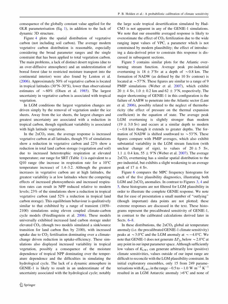
Fig. 4 Vegetation carbon (kgC m-2). LPC ensemble averages (left) and standard deviations (right). From top to bottom the plots illustrate the

modern state, the LGM anomaly and the 2xCO2 anomaly

P. B. Holden et al.: A probabilistic calibration of climate sensitivity

123

consequence of the globally constant value applied for the

OLR parameterisation (Eq. 1), in addition to the lack of

dynamic 3D structure.

Figure 4 plots the spatial distribution of vegetative

carbon (not including soil carbon). The average modern

vegetative carbon distribution is reasonable, especially

considering the broad parameter ranges and the single

constraint that has been applied to total vegetation carbon.

The main problems, a lack of distinct desert regions (due to

an over-diffusive atmosphere) and an underestimation of

boreal forest (due to restricted moisture transport into the

continental interior) were also found by Lenton et al.

(2006). Approximately 50% of vegetative carbon is located

in tropical latitudes (30�N–30�S), lower than observational

estimates of *60% (Olsen et al. 1985). The largest

uncertainty in vegetative carbon is associated with tropical

vegetation.

In LGM conditions the largest vegetation changes are

driven simply by the removal of vegetation under the ice

sheets. Away from the ice sheets, the largest changes and

greatest uncertainty are associated with a reduction in

tropical carbon, though significant variability is associated

with high latitude vegetation.

In the 2xCO2 state, the average response is increased

vegetative carbon at all latitudes, though 5% of simulations

show a reduction in vegetative carbon and 22% show a

reduction in total land carbon storage (vegetation and soil)

due to increased heterotrophic respiration at elevated

temperature; our range for SRT (Table 1) is equivalent to a

Q10 range (the increase in respiration rate for a 10�C

temperature increase) of 1.4–3.2. Although the greatest

increases in vegetative carbon are at high latitudes, the

greatest variability is at low latitudes where the competing

effects of increased photosynthesis and increased respira-

tion rates can result in NPP reduced relative to modern

levels; 23% of the simulations show a reduction in tropical

vegetative carbon (and 52% a reduction in tropical land

carbon storage). This equilibrium behaviour is qualitatively

similar to that exhibited by a range of transient (1850–

2100) simulations using eleven coupled climate-carbon

cycle models (Friedlingstein et al. 2006). These models

universally exhibited increased land carbon storage under

elevated CO2 (though two models simulated a sink/source

transition for land carbon flux by 2100), with increased

uptake due to CO2 fertilisation dominating over a climate-

change driven reduction in uptake-efficiency. These sim-

ulations also displayed increased variability in tropical

vegetation, possibly a consequence of the moisture

dependence of tropical NPP dominating over the temper-

ature dependence and the difficulties in simulating the

hydrological cycle. The lack of a dynamic atmosphere in

GENIE-1 is likely to result in an underestimate of the

uncertainty associated with the hydrological cycle; notably

the large scale tropical desertification simulated by Had-

CM3 is not apparent in any of the GENIE-1 simulations.

We note that our ensemble averaged response is likely to

overestimate the effect of CO2 fertilization due to the wide

ranging input values of VPC, a parameter which is not

constrained by modern plausibility; the effect of introduc-

ing a data-derived prior to constrain this response is dis-

cussed in subsequent sections.

Figure 5 contains similar plots for the Atlantic over-

turning stream function. Average peak pre-industrial

overturning is 18 ± 3�Sv at a depth of *0.8 km. The

formation of NADW (as defined by the 10 Sv contour) is

located at *57�N. These figures are similar to a range of 9

PMIP simulations (Weber et al. 2007), which exhibit

20 ± 4 Sv, 1.0 ± 0.2 km and 62 ± 3�N, respectively. The

major shortcoming of GENIE-1 in this configuration is the

failure of AABW to penetrate into the Atlantic sector (Lunt

et al. 2006), possibly related to the neglect of thermoba-

ricity (the effect of pressure on the thermal expansion

coefficient) in the equation of state. The average peak

LGM overturning is slightly stronger than modern

(19 ± 3.0 Sv) and occurs at a similar depth to modern

(*0.8 km) though it extends to greater depths. The for-

mation of NADW is shifted southward to *53�N. These

figures compare with PMIP averages, which also exhibit

substantial variability in the LGM stream function (with

unclear change of sign), to values of 20 ± 5 Sv,

1.1 ± 0.4 km, 55 ± 9�N (Weber et al. 2007). The average

2xCO2 overturning has a similar spatial distribution to the

pre-industrial, but exhibits a slight weakening to an average

peak of 17 ± 4 Sv.

Figure 6 compares the MPC frequency histograms for

each of the five plausibility diagnostics, illustrating both

LGM and 2xCO2 anomalies. In contrast to Figures 3, 4 and

5, these histograms are not filtered for LGM plausibility in

order to illustrate the complete GENIE response. We note

that for ease of presentation a small number of ‘‘outlying’’

(though important) data points are not plotted; these

extreme responses are discussed in the text. These histo-

grams represent the precalibrated sensitivity of GENIE-1,

in contrast to the calibrated calculations derived later in

Sects. 6–8.

In these distributions, the 2xCO2 global air temperature

anomaly (i.e. the precalibrated GENIE-1 climate sensitivity)

peaks at *3.0�C and the LGM anomaly at *-4.0�C. We

note that GENIE-1 does not generate DT2x below *2.0�C at

any point in our input parameter space. Although sufficiently

low values of KLW1 can generate arbitrarily low (positive)

climate sensitivities, values outside of our input range are

difficult to reconcile with the LGM plausibility constraint. In

initial exploratory ensembles, only 15 from 249 parame-

terisations with KLW1 in the range -0.5 to -1.0 W m-2 K-1

resulted in an LGM Antarctic anomaly [6�C and none of

P. B. Holden et al.: A probabilistic calibration of climate sensitivity

123

these 249 parameterisations produced an anomaly[9�C (cf

observational estimate 9 ± 2�C, Crucifix 2006). Notwith-

standing this, some caution should be exercised in inter-

preting our lower bound estimate for DT2x, especially given

that the neglect of dust is likely to have resulted in an Ant-

arctic warm bias of *1�C (Schneider von Deimling et al.

2006a). Furthermore, we note that lower values of DT2x

could be generated if the assumption of a constant feedback

parameter for LGM and 2xCO2 states breaks down, as is very

likely the case (Crucifix 2006); we discuss this assumption

further in Sect. 6 and account for it by incorporating an

explicit structural error term in Sect. 7.

The LGM-modern anomaly in Atlantic overturning

(defined as the maximum overturning stream function at

depths below *400 m) peaks at *2 Sv. Although the

distribution reflects a preference in GENIE-1 for a

strengthened LGM overturning, 29% of the simulations

exhibit a weakened LGM overturning. It is well known

(Weber et al. 2007) that models disagree on the sign of this

change, reflecting a balance of competing freshwater and

temperature effects on the density distribution. It is inter-

esting that this uncertainty in sign is demonstrated by a

single model, suggesting that much of this disagreement

may be arising from parametric uncertainty and therefore

may not reflect a fundamental difference between the

models themselves. In a 2xCO2 state, the distribution

reflects a strong preference for a slight weakening of

overturning. Nine of the 894 simulations exhibited a col-

lapse of the Atlantic overturning in a 2xCO2 state (as

defined by\10% of modern overturning strength). We note

that as we do not allow for the possibility of a Greenland

meltwater contribution to the freshwater balance, we are

likely to underestimate the probability of collapse, and the

magnitude of weakening in general. Conversely, four of the

simulations exhibit a substantial strengthening of Atlantic

overturning (*5–10 Sv), though in each case the modern

Modern Average Atlantic Overturning

-20 0 20 40 60 80-5

-4

-3

-2

-1

0

-5 0 5 10 15 20

Modern Atlantic Overturning Standard Deviation

-20 0 20 40 60 80-5

-4

-3

-2

-1

0

0 1 2 3 4 5 6

LGM Average Atlantic Overturning Anomaly

-20 0 20 40 60 80-5

-4

-3

-2

-1

0

-5 -4 -3 -2 -1 0 1 2 3 4 5

Standard Deviation of LGM Atlantic Overturning Anomaly

-20 0 20 40 60 80-5

-4

-3

-2

-1

0

0 1 2 3 4 5 6

2xCO2 Average Atlantic Overturning Anomaly

-20 0 20 40 60 80-5

-4

-3

-2

-1

0

-5 -4 -3 -2 -1 0 1 2 3 4 5

Standard Deciation of 2xCO2 Atlantic Overturning Anomaly

-20 0 20 40 60 80-5

-4

-3

-2

-1

0

0 1 2 3 4 5 6

0

-1

0 0

0 1 2 3 4 5 6

0 40-5

-4

-3

-2

-1

0

-1 0 1 2 3 4 5

0-5

-4

-3

-2

-1

0

0 1 2 3 4 5 6

0-5

-1

0

-1 0 1 2 3 4 5

0-5

-4

-3

-2

-1

0

0 1 2 3 4 5 6

Fig. 5 Atlantic Overturning

stream function (Sv). LPC

ensemble averages (left) and

standard deviations (right).From top to bottom the plots

illustrate the modern state, the

LGM anomaly and the 2xCO2

anomaly

P. B. Holden et al.: A probabilistic calibration of climate sensitivity

123

distribution is unrealistic, shifted very far southwards to

*25�N with greatly weakened North Atlantic deep

convection.

The increase in annually-averaged LGM sea–ice area

peaks at *9 million km2 in the Antarctic and *7 mil-

lion km2 in the Arctic, though substantial uncertainty is

exhibited. In a 2xCO2 state, sea–ice loss peaks at *6 mil-

lion km2 in the Antarctic and *3 million km2 in the Arctic.

The small probability of an increase in Arctic sea ice is

associated with the occasional collapse of Atlantic over-

turning and the associated reduction of northward heat

transport. The Arctic remains ice-free throughout the year

in *5% of the 2xCO2 simulations, at least in part due to our

low resolution, though these parameterisations are all

associated with low sea–ice cover in the modern state (with

an annual average of 4.4 million km2).

LGM reductions in vegetative carbon *150 GtC and

soil carbon *450 GtC are consistent with a range of data

and model estimates (Peng et al. 1998) of *30% reduction

in land carbon storage. Although the 2xCO2 distribution of

vegetative carbon strongly favours an increase from

modern values (with only 4% simulations exhibiting a

reduction), the soil carbon distribution reflects change of an

unclear sign (with 29% of simulations exhibiting a reduc-

tion), driven by competing effects of an increased source

(vegetation carbon) and increased respiration rates in a

warmer world. The MPC distribution for total land carbon

storage change under doubled CO2 is 250 ± 294 GtC.

In summary, we have demonstrated that our experi-

mental design has produced an average climate state that is

reasonably well centred on modern observations, but which

exhibits a wide range of responses to both LGM and 2xCO2

forcing, a range which encompasses much of the differing

behaviour that is observed in more complex models.

5 An emulation of climate sensitivity

In order to investigate the interactions between parameters

and to quantify the contribution of the individual parame-

terisations to climate sensitivity in GENIE-1, we built a

deterministic emulator for DT2x, following the procedure

Global average SAT anomaly °C

0%

5%

10%

15%Atlantic Overturning anomaly (Sv)

0%

5%

10%

15%

Arctic Sea ice area anomaly (million km2)

0%

5%

10%

15%

20%

25%

Vegetation carbon anomaly (GTC)

0%

5%

10%

15%

Antarctic Sea ice area anomaly (million km2)

0%

5%

10%

15%

Soil carbon anomaly (GTC)

0%

5%

10%

15%

0%

5%

10%

15%

0%

5%

10%

15%

)

0%

5%

10%

15%

20%

25%

0%

5%

10%

15%

0%

5%

10%

15%

0%

5%

10%

15%

-10 -9 -8 -7 -6 -5 -4 -3 -2 -1 0 1 2 3 4 5 6 7 -5 -4 -3 -2 -1 0 1 2 3 4 5 6 7

-6 -4 -2 0 2 4 6 8 10 12 14

-250 -210 -170 -130 -90 -50 -10 30 70 110 150 190 230

-12 -10 -8 -6 -4 -2 0 2 4 6 8 10 12 14 16 18 20 22 24

-1000 -800 -600 -400 -200 0 200 400 600 800 1000

Fig. 6 MPC Frequency histograms for LGM anomalies (blue) and 2xCO2 anomalies (orange). Some extreme ‘‘outlying’’ values are omitted for

ease for presentation but are discussed in the text

P. B. Holden et al.: A probabilistic calibration of climate sensitivity

123

described in Sect. 3. The emulator was built from the MPC

parameter set; the LGM plausibility constraint was not

applied in order to maximise the range of the response.

After an initial emulation was performed including qua-

dratic terms for the 25 active parameters (the quadratic

emulator), five of the least significant parameters, based

on this and an earlier model, were excluded and the com-

plexity of allowed emulator interactions increased to

include cubic terms (the cubic emulator). The cubic emu-

lator exhibited a standard error (the standard deviation of

the discrepancy between emulated and simulated climate

sensitivity) of ±0.12�C and an R2 of 97.4%. As a check

against over-fitting, a second cubic emulator (cubic_600)

was built with an identical methodology but from a random

subset of 600 of the MPC parameter vectors. The remaining

294 members were used as a validation set, and displayed a

cross-validated standard error of ±0.16�C. The R2 between

the 85 coefficients of the cubic emulator and their equiva-

lent coefficient (zero if absent) in the cubic_600 emulator is

71%, suggesting the dominant terms can be regarded as a

reasonably robust representation of GENIE-1.

The emulators allow us to investigate the uncertainty in

DT2x as a function of the input parameters. As in Sect. 3, we

achieve this through a global sensitivity analysis, calculat-

ing the total effect of each parameter, which provides a

measure of the contribution of that parameter to the vari-

ance in emulated climate sensitivity (Eq. 4). We do not

calculate the total effect analytically (as in Sect. 3) but

approximate the integral by averaging over the Latin

Hypercube (D) and over the LPC parameter set (Table 3).

The Latin Hypercube calculation describes the apportion-

ment of variance given the initial uniform independent prior

ranges summarised in Table 1. The LPC calculation illus-

trates the constraining effect of modern and LGM plausi-

bility. Table 3 summarises the Latin Hypercube calculation

under various assumptions. The main result is the 1st data

column which tabulates the square root of the total effect (as

a measure of the 1r variation) in the cubic emulation. The

following three columns test the robustness of this result by

calculating the total effect for (1) the cubic emulator over a

subset of 500 of the Latin Hypercube members (to test

for convergence of the approximate calculation of VkT), (2)

the cubic_600 emulator and (3) the quadratic emulator.

Integrating the emulator over uniform priors requires

extrapolating beyond the narrow plausible regions (of 26-

dimensional space) that were used to train the emulator.

However, these four calculations all provide similar results,

suggesting the apportionment of variance to the parameters

is robust. The similar results for the cubic and quadratic

emulators suggest that three-way interactions are not sig-

nificant. We note that the emulators achieve this similar

apportionment of variance through different combinations

of cross-terms, suggesting that the details of the individual

interactions may be difficult to interpret unambiguously.

Interactions introduced in the MPC parameter set

through the enforcement of modern plausibility introduce

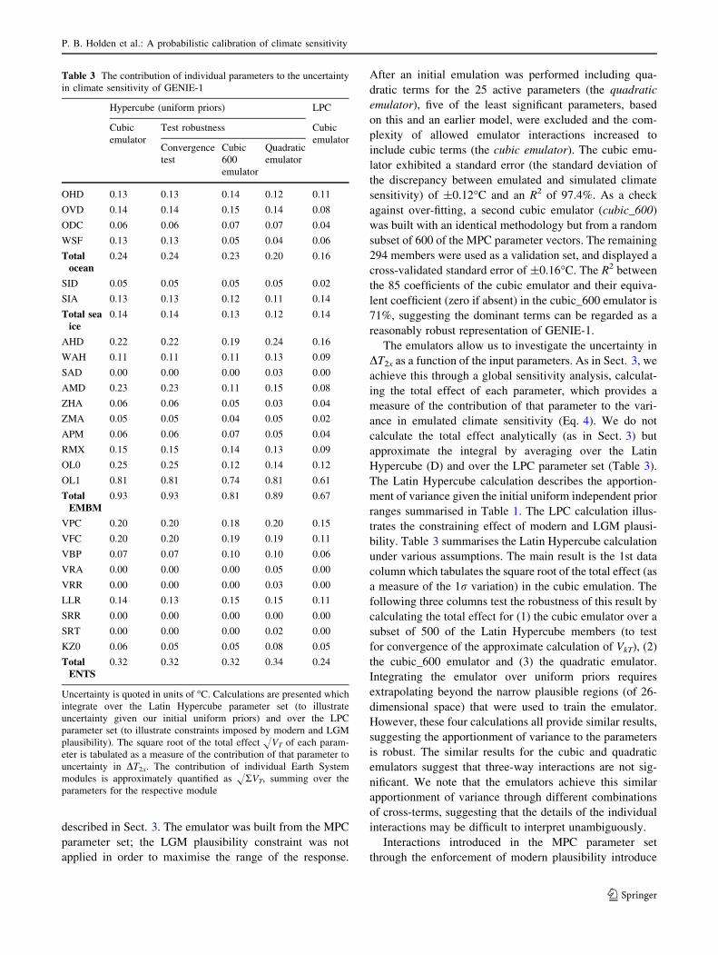
Table 3 The contribution of individual parameters to the uncertainty

in climate sensitivity of GENIE-1

Hypercube (uniform priors) LPC

Cubic

emulator

Test robustness Cubic

emulatorConvergence

test

Cubic

600

emulator

Quadratic

emulator

OHD 0.13 0.13 0.14 0.12 0.11

OVD 0.14 0.14 0.15 0.14 0.08

ODC 0.06 0.06 0.07 0.07 0.04

WSF 0.13 0.13 0.05 0.04 0.06

Totalocean

0.24 0.24 0.23 0.20 0.16

SID 0.05 0.05 0.05 0.05 0.02

SIA 0.13 0.13 0.12 0.11 0.14

Total seaice

0.14 0.14 0.13 0.12 0.14

AHD 0.22 0.22 0.19 0.24 0.16

WAH 0.11 0.11 0.11 0.13 0.09

SAD 0.00 0.00 0.00 0.03 0.00

AMD 0.23 0.23 0.11 0.15 0.08

ZHA 0.06 0.06 0.05 0.03 0.04

ZMA 0.05 0.05 0.04 0.05 0.02

APM 0.06 0.06 0.07 0.05 0.04

RMX 0.15 0.15 0.14 0.13 0.09

OL0 0.25 0.25 0.12 0.14 0.12

OL1 0.81 0.81 0.74 0.81 0.61

TotalEMBM

0.93 0.93 0.81 0.89 0.67

VPC 0.20 0.20 0.18 0.20 0.15

VFC 0.20 0.20 0.19 0.19 0.11

VBP 0.07 0.07 0.10 0.10 0.06

VRA 0.00 0.00 0.00 0.05 0.00

VRR 0.00 0.00 0.00 0.03 0.00

LLR 0.14 0.13 0.15 0.15 0.11

SRR 0.00 0.00 0.00 0.00 0.00

SRT 0.00 0.00 0.00 0.02 0.00

KZ0 0.06 0.05 0.05 0.08 0.05

TotalENTS

0.32 0.32 0.32 0.34 0.24

Uncertainty is quoted in units of �C. Calculations are presented which

integrate over the Latin Hypercube parameter set (to illustrate

uncertainty given our initial uniform priors) and over the LPC

parameter set (to illustrate constraints imposed by modern and LGM

plausibility). The square root of the total effect HVT of each param-

eter is tabulated as a measure of the contribution of that parameter to

uncertainty in DT2x. The contribution of individual Earth System

modules is approximately quantified as HRVT, summing over the

parameters for the respective module

P. B. Holden et al.: A probabilistic calibration of climate sensitivity

123

correlations between parameters. In general these are weak,

but three parameter pairs are highly correlated: OL0/RMX

(R2 = 74%, negatively correlated as increases in either

leads to reduced OLR, with similar effects on modern SAT

plausibility), SRT/SRR (R2 = 34%, positively correlated

through their opposing effects on soil carbon) and AMD/

APM (R2 = 30%, positively correlated through their

competing effects on North Atlantic surface salinity and

hence on Atlantic overturning). As a consequence, the

apportionment of variance between these paired parameters

may not be robust. Notably, we cannot rule out the possi-

bility that all of the uncertainty ascribed jointly to OL0 and

RMX (HRVT = 0.30�C) is driven entirely by uncertainties

in RMX; physical considerations suggest OL0 is unlikely

to contribute to uncertainty in climate sensitivity as it

represents OLR uncertainty in the modern state (Eq. 1) and

has no clear feedback role (whereas RMX exerts influence

on the water vapour feedback by limiting relative humid-

ity). However, as all three parameter pairs are within the

same module (atmosphere, vegetation and atmosphere

respectively), this does not affect the apportionment of

uncertainty between modules discussed below.

This procedure ascribes 85% of the variance to the

EMBM parameters, associated with an approximate 1rerror of ±0.93�C (Table 3, calculated as HRVT summed

over the EMBM parameters, and providing an upper bound

as the summed total effect is always greater than the total

variance). Although dominated by atmospheric processes,

the variance associated with other modules indicates that

they are not negligible and contribute approximate 1rerrors of ±0.32�C (vegetation), ±0.24�C (ocean) and

±0.14�C (sea–ice). For comparison, a cubic emulator built

from all 26 parameters provided error contributions of

0.88�C (EMBM), 0.40�C (ENTS), 0.22�C (ocean) and

0.16�C (sea ice). Note the low uncertainty associated with

sea–ice parameterisations does not imply a weak sea–ice

feedback; uncertainty in the sea–ice feedback is dominated

by uncertainties in sea–ice area which in turn are domi-

nated by uncertainties in ocean and atmospheric transport

rather than the sea–ice parameterisations themselves (see

Fig. 2). In general, it is not trivial to associate particular

parameterisations with individual feedback mechanisms.

Figure 7 plots the dominant emulator interactions. Only

parameters which contribute more than 1% to the total

variance were considered and only interactions large

enough to change the emulated climate sensitivity by more

that the standard error are included. A single three-way

interaction (OHD:OL1:LLR) was additionally excluded as

this interaction was not present in the cubic_600 emulator

and thus may not be considered robust when viewed in

isolation. The strong interactions plotted are unlikely to

represent an over-fitting to the model output, though we

cannot rule out the possibility that the correlations in input

space noted earlier may influence these interactions. It is

apparent that the strongest inter-module interactions (con-

trolling climate sensitivity) take place through the EMBM.

The dominant parameter is OL1, which crudely para-

meterises the role of cloud and lapse rate feedbacks.

Atmospheric moisture diffusivity is notable in that it does

not affect climate sensitivity directly (i.e. through a linear

term), but is strongly coupled to the rest of the system and,

in particular, interacts strongly with feedbacks in vegeta-

tion and atmospheric humidity.

6 Introducing a probabilistic LGM data constraint

In order to calculate posterior probability distributions for

climate, we first derive posterior probability weightings for

the parameter vectors by applying an LGM constraint and

subsequently apply these weightings to the precalibrated

distributions of Fig. 5; note this calibration is performed

upon the simulator (GENIE-1) output, not the emulated

output. This section describes the analytical approach,

including a discussion of the base case (Sect. 7, Assump-

tion A7) structural error assumptions applied. The

Fig. 7 The climate sensitivity emulator. The four GENIE modules

are grouped separately: EMBM atmosphere (turquoise), GOLD-

STEIN ocean (blue), sea ice (grey) and ENTS vegetation (green). The

filtering process to select terms is described in the text. The 1r error

contributions for each module are approximated as the square root of

the sum of the total effects HR VT of the parameterisations in that

module (Table 4). Red circles are positive linear terms which

contribute more than the standard error of the emulator when the

parameter is varied across its input range. Blue circles are negative

linear terms. Medium sized circles contribute more than twice the

standard error of the emulator. Large circles (OL1) contribute more

than four times the standard error. Lines represent interactions which

contribute more than the standard error; thick lines contribute more

than twice the standard error. Reverse arrows represent quadratic

terms which are positive (red) or negative (blue)

P. B. Holden et al.: A probabilistic calibration of climate sensitivity

123

calculation of climate sensitivity, including a sensitivity

analysis to the structural error assumptions is performed in

Sect. 7.

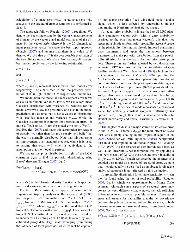
The approach follows Rougier (2007) throughout. We

denote the true climate state by the vector y, measurements

of climate by the vector z and model estimates of the cli-

mate by the vector g(h), where h is the 26 dimensional

input parameter vector. We take the best input approach

(Rougier 2007) and assume that there is a value of h,

denoted h*, such that g(h*) is the best possible prediction of

the true climate state y. We relate observations, climate and

best model prediction by the following relationships

z ¼ yþ eo ð6Þ

and

y ¼ gðh�Þ þ es ð7Þ

where eo and es represent measurement and model error

respectively, The aim is then to find the posterior distri-

bution of h* in light of the LGM tropical SST anomalies.

We model both the model and measurement error terms

as Gaussian random variables. For eo we use a zero-mean

Gaussian distribution with variance ro, whereas for the

model error we allow the possibility of a bias in the model

predictions and assume that es has a Gaussian distribution

with specified mean l and variance rLGM. While the

Gaussian assumption is common for observation error, it is

more difficult to justify for the model error term. We fol-

low Rougier (2007) and make this assumption for reasons

of tractability, rather than for any strongly held belief that

the error is normally distributed. Note that this represents

an improvement over standard practice, where it is usual

to assume that rLGM = 0 which is equivalent to the

assumption that the model is perfect.

We update the prior distribution in light of the LGM

constraint zLGM to find the posterior distribution, using

Bayes’ theorem (Rougier 2007, Eq. 7):

Prðh�jzLGM ¼ ~zLGMÞ¼ cuð~zLGM � gLGMðh�Þ; l; ro þ rLGMÞpðh�Þ

ð8Þ

where /(.) is the Gaussian density function with specified

mean and variance, and c is a normalising constant.

For the LGM constraint, we apply the result of the

Bayesian multi-proxy analysis of Ballantyne et al. (2005)

for tropical SST anomalies of 2.7 ± 0.5�C. i.e.

~zLGM(observed LGM tropical SST anomaly) = 2.7�C,

Hro = 0.5�C, where gLGM(h*) is the modelled LGM

tropical SST anomaly with error (l, rLGM). The choice of a

tropical SST constraint is discussed in some detail in

Schneider von Deimling et al. (2006a), favoured by well-

calibrated proxy data, large scale averaging (minimising

the influence of local processes which cannot be captured

by our coarse resolution fixed wind-field model) and a

signal which is less affected by uncertainties in the

topography of Northern hemisphere ice sheets.

An equal prior probability is ascribed to all LPC plau-

sible parameter vectors p(h) (with a zero probability

ascribed to the other parameter vectors); this does not

represent a simple uniform prior probability across h space

as the plausibility filtering has already imposed constraints

upon parameters and upon the interactions between

parameters; i.e. the posterior distribution from the plausi-

bility filtering forms the basis for our prior assumption

here. These priors are further adjusted by two data-driven

estimates. VPC is constrained by the compilation of CO2

fertilisation data of Wullshleger et al. (1995) which implies

a Gaussian distribution of / (145, 200) ppm for the

Michaelis-Menton half saturation; plausibility tests do not

constrain this response and the photosynthesis data suggest

the lower end of our input range (0–700 ppm) should be

favoured. A prior is applied for oceanic isopycnal diffu-

sivity, also poorly constrained by modern plausibility,

assumed to be a gamma distribution (a = 2, b = 1,000)

m2 s-1, exhibiting a mode of 1,000 m2 s-1 and a mean of

2,000 m2 s-1. Our choice of mode represents the canonical

value for vertically constant isopycnal diffusivity (as

applied here), though this value is associated with sub-

stantial uncertainty and spatial variability (Ferreira et al.

2005).

The neglect of dust is a major source of structural error

in the LGM SST anomaly rLGM; the main effect of LGM

dust was a likely cooling in the tropics (Claquin et al.

2003). Schneider von Deimling et al. (2006a) incorporated

dust fields and implied an additional tropical SST cooling

of 0.4–0.9�C. As the absence of dust introduces a bias, as

well as an uncertainty, we incorporate this by applying a

non-zero mean l of 0.6�C to the structural error, in addition

to HrLGM = 1.0�C. Though we describe the absence of a

coupled dust model as a source of structural error, we note

that it could equally be described as an absent forcing; the

analytical approach is not affected by this distinction.

A probability distribution for climate sensitivity yDT2xcan

then be found using the law of total probability (Rougier

2007, Eq. 8), which we approximate by a Monte Carlo

estimate. Although some aspects of structural error may

covary between different climate states, we lack sufficient

information to estimate all possible sources of structural

error and assume for tractability that the net covariance

between the paleo-climate and future climate state, in both

measurement error and structural error, is zero (see Rougier

2007, Sect. 6.3). In this case

PrðyDT2xjLGMÞ ¼

XLPC

uðyDT2x� gDT2x

ðh�Þ; lCS; rCSÞ

� Prðh�jLGMÞ ð9Þ

P. B. Holden et al.: A probabilistic calibration of climate sensitivity

123

where we sum over the LPC parameter set, applying the

posterior probabilities Pr(h|LGM) derived in Eq. 8. Here

we have assumed the model error in our constrained cal-

culation of DT2x is Gaussian with mean lCS (assumed to be

zero) and variance rCS. These quantities are distinct from

lCS and rLGM which represent the structural error in the

modelling of the LGM constraint. We also apply this

equation in its more general form (i.e. climate yV, model

output gV(h*) and structural error mean lV and variance rV)

to derive 2xCO2 and LGM probability distributions for

other output variables in Sect. 8.

The structural error rCS in the calculation of DT2x is

arguably likely to be dominated by the assumption of a

constant OL1 feedback parameter. Schneider von Deimling

et al. (2006a) found a very close correlation between LGM

tropical SST anomalies and DT2x using CLIMBER-2.

These results suggest the assumption of a constant feed-

back parameter introduces a 2r structural error in DT2x of

only *0.25�C. However, the correlation between LGM

and 2xCO2 states was found to be substantially weaker in

an AGCM coupled to a slab ocean (Annan et al. 2005),

suggesting a 1r structural error of *0.8�C is more

appropriate. PMIP2 simulations (Masson-Delmotte et al.

2006) suggest an approximately linear relationship

between forcing and temperature change between LGM

and 4xCO2 forcing. However, this result may be a reflec-

tion of averaging over differing model responses; Crucifix

(2006) compared the results of the 4 PMIP2 GCMs which

were applied to both LGM and 2xCO2 states and found that

the assumption of constant feedback parameters for LGM

and DT2x may break down, primarily due to the non-linear

response of subtropical shallow convective clouds to tem-

perature change. We here apply a 1r structural error

HrCS = 0.8�C, noting that this range is greater that the

standard deviation (±0.7�C) of the 19 GCM equilibrium

climate sensitivities in IPCC (2007), differences which

primarily reflect differing cloud and lapse rate feedbacks.

A broader structural error assumption of HrCS = 1.2�C is

also included for comparison.

Figure 8 is a scatterplot of DT2x versus LGM tropical

SST anomalies; open circles are the 894 MPC parameter

vectors and filled circles are the subset of 480 LPC

parameter vectors. The vertical lines represent the 1robservational estimate of Ballantyne et al. (2005). The

dashed lines are the 2r RMS deviation from a straight line

fit to the LPC simulations. The 2r uncertainty of ±0.9�C

compares to ±0.25�C (Fig. 6 of Schneider von Deimling

et al. 2006a) and ±1.6�C (ACGM ensemble, Fig. 2 of

Annan et al. 2005); although our precalibration approach

has captured much of the uncertainty associated with

asymmetric responses to warming and cooling climate, the

lack of a dynamic atmosphere inevitably fails to capture all

of the uncertainty apparent in the AGCM ensemble. We

note that the structural error term HrCS = 0.8�C is pri-

marily designed to allow for the asymmetric atmospheric

feedbacks which GENIE-1 cannot capture.

7 Probability distribution for climate sensitivity

We derive posterior distributions for climate sensitivity

under a range of assumptions (A1–A10), summarised in

Table 4. The purpose here is to investigate the robustness

of our conclusions with respect to the partially subjective

choices that we are required to make in our Bayesian

analysis. We note that such subjective choices are invari-

ably required in a complex statistical analysis; one benefit

of a Bayesian approach is to make these choices explicit

and provide a quantification of their role. Our ‘‘best’’

estimate A7 (applying the assumptions described in

Sect. 6) is in bold face. The alternative analyses are:

(A1) Neither LGM nor prior constraints are imposed

(the calculation is derived from the MPC param-

eter set) and an allowance for structural error is

not incorporated into the calibration (though we

assume a small structural error of HrCS = 0.2�C

in KLW1 which acts to smooth the posterior).

Unconstrained GENIE-1 climate sensitivity peaks

at 3.0�C, likely in the range 2.8–4.4�C. This

assumption is (the smoothed) equivalent of the

precalibrated climate sensitivity plotted in the

histogram in Fig. 2, and is plotted as the light

orange line in the first panel of Fig. 9.

(A2) The introduction of priors (see Sect. 6) for CO2

fertilisation (VPC) and isopycnal diffusivity

2

3

4

5

6

7

-10 -8 -6 -4 -2 0

LGM Tropical SST Anomaly °C

Clim

ate

Sen

siti

vity

°C

Fig. 8 Scatterplot of climate sensitivity against LGM tropical SST

anomaly. Open circles are the MPC parameter set and filled circlesthe LPC parameter set (a subset of MPC but filtered for LGM

Antarctic SAT plausibility). Solid vertical lines are the 1r range of

the multi-proxy paleodata (Ballantyne et al. 2005) applied as the

LGM constraint. Dashed lines are the 2r RMS scatter about a straight

line fit to the 480 LPC simulations, representing an uncertainty of

±0.9�C

P. B. Holden et al.: A probabilistic calibration of climate sensitivity

123

(OHD) has little effect on DT2x, reducing the most

likely value to 2.9�C. This is dominantly a

consequence of reduced photosynthesis and, pre-

sumably, the resulting increase in land surface

albedo.

(A3) The introduction of LGM constraints (still neglect-

ing structural error) by incorporating the LPC

priors and constraining with LGM tropical SST

markedly narrows the uncertainty. The LGM

constraint shifts the most probable climate sensi-

tivity upwards to 3.5�C as less sensitive climates

are generally less able to reproduce the observed

LGM cooling.

(A4) Introducing a structural error assumption of

HrLGM = 1.5�C in LGM tropical SSTs in the

calibration stage increases the most probable

climate sensitivity to 3.7�C. This reflects the

increased influence of extreme cooling responses

(associated with increased sensitivity) in the long

tail of the distribution, which are less strongly

disfavoured under the assumption of a large model

error.

(A5) Introducing a structural error of HrCS = 0.8�C

(the assumption of a constant feedback parameter

KLW1) (with rLGM = 0) substantially increases the

uncertainty in DT2x, but does not affect the peak of

the distribution. The effect of this error term is to

weaken the LGM constraint imposed on KLW1 and

hence to broaden the estimate of DT2x; it does not

affect the probabilities ascribed to parameter

vectors in the calibration stage and hence has

little affect on the ‘‘peak-shifting’’ driven by the

LGM constraint.

(A6) The combined effect of both sources of structural

error rLGM and rCS (A4 and A5) is a broadened

distribution, shifted towards a higher climate

sensitivity.

(A7) A bias is introduced into the structural error at the

calibration stage (l = 0.6�C) to reflect the neglect

of dust and the resulting warm-bias in LGM

tropical SSTs. We reduce our structural error

assumption to HrLGM = 1.0�C, reflecting our

increased confidence now that the structural bias

due to the neglect of dust has been accounted for.

The incorporation of a bias term shifts the

probability distribution to lower climate sensitiv-

ities; the ‘‘optimum’’ model response is shifted

towards warmer LGM SSTs (which would be

cooled by the presence of dust), thus favouring

parameterisations which exhibit lower sensitivi-

ties. The introduction of dust biasing has little

impact upon the calculated climate sensitivity as a

consequence of the conservative structural errorTa

ble

4B

ayes

con

stra

ined

clim

ate

sen

siti

vit

y;

Ass

um

pti

on

sA

1–

A1

0

LG

Mco

nst

rain

tP

aram

eter

pri

ors

LG

Mb

ias

l(�

C)

Str

uct

ura

ler

ror

LG

Mco

nst

rain

t

Hr

LG

M(�

C)

Str

uct

ura

lE

rro

rK

LW

1

extr

apo

lati

onH

r CS

(�C

)

Mo

stli

kel

y

clim

ate

sen

siti

vit

y(�

C)

66

%C

on

fid

ence

inte

rval

(ran

ge)

(�C

)

90

%C

on

fid

ence

inte

rval

(ran

ge)

(�C

)

1N

on

eM

PC

No

N/A

0.2

3.0

2.8

–4

.4(1

.6)

2.4

–5

.1(2

.7)

2N

on

eM

PC

&V

PC

,O

HD

No

N/A

0.2

2.9

2.7

–4

.3(1

.6)

2.4

–5

.0(2

.6)

3P

lau

sib

ilit

yan

dtr

op

ical

SS

TL

PC

&V

PC

,O

HD

No

00

.23

.53

.0–

3.9

(0.9

)2

.8–

4.2

(1.5

)

4P

lau

sib

ilit

yan

dtr

op

ical

SS

TL

PC

&V

PC

,O

HD

No

1.5

0.2

3.7

3.1

–4

.2(1

.1)

2.8

–4

.6(1

.8)

5P

lau

sib

ilit

yan

dtr

op

ical

SS

TL

PC

&V

PC

,O

HD

No

00

.83

.52

.6–

4.3

(1.7

)2

.0–

4.9

(2.9

)

6P

lau

sib

ilit

yan

dtr

op

ical

SS

TL

PC

&V

PC

,O

HD

No

1.5

0.8

3.7

2.8

–4

.6(1

.8)

2.1

–5

.2(3

.1)

7P

lau

sib

ilit

yan

dtr

op

ical

SS

TL

PC

&V

PC

,O

HD

0.6

1.0

0.8

3.6

2.6

–4

.4(1

.8)

2.0

–5

.0(3

.0)

8T

rop

ical

SS

TM

PC

&V

PC

,O

HD

0.6

1.0

0.8

3.1

2.2

–4

.0(1

.8)

1.6

–4

.7(3

.1)

9E

ast

An

tarc

tic

SA

TM

PC

&V

PC

,O

HD

1.0

2.0

0.8

3.5

2.6

–4

.5(2

.0)

1.9

–5

.2(3

.4)

10

Pla

usi

bil

ity

and

tro

pic

alS

ST

LP

C&

VP

C,

OH

D0

.61

.01

.23

.62

.3–

4.7

(2.4

)1

.4–

5.6

(4.2

)

P. B. Holden et al.: A probabilistic calibration of climate sensitivity

123

assumptions which serve to weaken the LGM

constraint. Assumption A7 represents our favoured

assumption set for DT2x as likely to lie between 2.6

and 4.4�C, with a peak probability at 3.6�C.

(A8) For comparison, the same assumptions are applied

to the MPC parameter set. It is apparent that

removing the LGM Antarctic plausibility test

would largely reconcile the 90% confidence

interval (1.6–4.7�C) with the CLIMBER-2 esti-

mate of 1.2–4.3�C (Schneider von Deimling et al.

2006a).

(A9) For further comparison we apply the alternative

LGM constraint of the East Antarctic SAT anom-

aly (9.0 ± 2.0�C, Crucifix 2006) as favoured by

Hargreaves et al. (2007). To avoid double count-

ing of the Antarctic SAT constraint, we here

perform the Monte Carlo integration over the

MPC parameter set (which is not filtered for LGM

Antarctic plausibility). We assume an increased

structural error of HrLGM = 2�C, reflecting addi-

tional uncertainty due to polar amplification, and

an Antarctic dust-induced bias of l = 1.0�C

(Schnieder von Deimling et al. 2006b). This

analysis produces a similar climate sensitivity

than the tropical SST constraint, peaking at 3.5�C

and likely to lie between 2.6 and 4.5�C. We note

that the application of the Antarctic constraint

introduces additional uncertainties (especially

given our simplified atmosphere), primarily due

to changes in ice-sheet topography (Krinner and

Genthon 1998), but include this analysis as a

useful validation of the robustness of our results.

(A10) For further comparison, we include an SST

constrained calculation with a more conservative

structural error assumption for KLW1 HrCS =

1.2�C. This does not affect our estimate of the

most probable climate sensitivity, but broadens the

likely range to lie between 2.3 and 4.7�C.

Atlantic Overturning anomaly (Sv)

0.0

0.1

0.2

0.3

0.4

-7 -5 -3 -1 1 3 5 7

Arctic Sea ice area anomaly (million km2)

0.0

0.1

0.2

0.3

0.4

-6 -4 -2 0 2 4 6 8 10 12 14

Antarctic Sea ice area anomaly (million km2)

0.0

0.1

0.2

-12 -8 -4 0 4 8 12 16 20 24

Soil carbon anomaly (GTC)

0.E+00

1.E-03

2.E-03

-1000 -800 -600 -400 -200 0 200 400 600 800 1000

Vegetation carbon anomaly (GTC)

0.00

0.01

-250 -200 -150 -100 -50 0 50 100 150 200 250

Global average SAT anomaly °C

0.0

0.1

0.2

0.3

0.4

0.5

0.6

-10 -8 -6 -4 -2 0 2 4 60.0

0.1

0.2

0.3

0.4

-7 -5 -3 -1 1 3 5 7

0.0

0.1

0.2

0.3

0.4

-6 -4 -2 0 2 4 6 8 10 12 14

0.0

0.1

0.2

-12 -8 -4 0 4 8 12 16 20 24

0.E+00

1.E-03

2.E-03

0.00

0.01

0.0

0.1

0.2

0.3

0.4

0.5

0.6

-10 -8 -6 -4 -2 0 2 4 6

Fig. 9 Probability distributions for LGM and 2xCO2 climate states. LGM (blue) and 2xCO2 (orange). Light lines illustrate the unconstrained

distributions (Assumption A1) and dark lines the fully constrained posterior distributions (Assumption A7)

P. B. Holden et al.: A probabilistic calibration of climate sensitivity

123

8 Probability distributions of LGM and 2xCO2 climate

states

Figure 9 illustrates the climate state posterior distributions

for LGM and 2xCO2 climate states, comparing the

unconstrained distributions (Assumption A1) with the fully

constrained distributions (Assumption A7). These com-

parisons illustrate the combined effects of the LGM trop-

ical SST constraint, allowing for structural error, and the

data-driven parameter priors for CO2 fertilization and iso-

pycnal diffusivity.

For fully constrained calculations, the structural error for

LGM air temperature is assumed to be HrV = 0.8�C, the

same value as was assumed for 2xCO2, though likely more

conservative as it does not rely upon the assumption of a

constant feedback parameter. As we are likely to underes-

timate LGM cooling due to the neglect of dust, we introduce

this bias through lV = 1.0�C (Schneider von Deimling et al.

2006b). The resulting estimate for LGM cooling of 6.2�C,

likely in the range 5.3–7.5�C, is similar to the CLIMBER-2

estimate (Schneider von Deimling et al. 2006b) of

5.8 ± 1.4�C (2r). The CLIMBER-2 result was reconciled

with PMIP-2 simulations (4.1 ± 1.0�C, Masson-Delmotte

et al. 2006) by considering additional cooling of *1.5�C

due to the combined effects of dust and vegetation, both of

which were neglected in the PMIP-2 study.

For other output no bias is assumed (lV = 0), but

structural error HrV was applied for Atlantic overturning

(1 Sv), Arctic/Antarctic sea–ice area (1 million km2),

vegetation carbon (25 GtC) and soil carbon (100 GtC).

Structural error is more difficult to estimate for these dis-

tributions, so we simply apply these minimal values in order

to smooth the posteriors. The justification for this is that we

have attempted to allow for structural error in these quan-

tities through our ensemble design. The fully constrained

distributions are summarised quantitatively in Table 5. The

unconstrained distributions also include a minimal struc-

tural error assumption. These values are identical to those

above, with a value of HrV = 0.2�C for air temperature,

which is applied as a smoothing term to both LGM and

2xCO2 states. Aside from the smoothing effect of the

structural error term, the unconstrained distributions are

directly comparable to the frequency histograms in Fig. 6.

Changes in land carbon storage are especially note-

worthy. Under LGM conditions, the peak probability for

land carbon storage change is a reduction by 470 GTC

from modern values, likely in the range 330–700 GTC (this

calculation assumes the complete removal of land carbon

under ice-sheets). Under 2xCO2, the change in equilibrium

land carbon storage is of unclear sign, with a peak proba-

bility at 30 GTC, likely to lie in the range -160 to ?350

GTC, with a 37% probability terrestrial carbon is reduced

from modern values, so that land has turned from a sink to

a source of atmospheric CO2. These figures are sensitive to

the constraint imposed by the prior distribution for CO2

fertilisation (see Sect. 6). Assuming a uniform prior dis-

tribution for VPC from 0 to 700 ppm (Table 1), likely to

overstate the effect of CO2 fertilisation, the probability of a

sink/source transition under elevated CO2 is 24%. Note that

additional constraints could be imposed through priors on

other parameterisations, notably the respiration response to

temperature.

Although the ensemble design has allowed a wide range

of responses, it does not allow for all sources of structural

Table 5 Posterior distributions

for LGM and 2xCO2 climate

states

Peak probability Likely range (66%) Very likely range (90%)

LGM anomaly

Global SAT (�C) -6.2 -5.3 to -7.5 -4.6 to -8.3

Atlantic overturning (Sv) -0.4 -2.0 to 2.6 -3.4 to 4.6

Arctic sea ice (million km2) 8.0 6.0–10.2 4.2–12.0

Antarctic sea ice (million km2) 10.6 9.2–15.4 7.6–17.8

Vegetation carbon (GTC) -142 -108 to -186 -80 to -215

Soil carbon (GTC) -340 -200 to -540 -70 to -670

Total land carbon (GTC) -470 -330 to -700 -180 to -830

2xCO2 anomaly

Global SAT (�C) 3.6 2.6–4.4 2.0–5.0

Atlantic overturning (Sv) -0.7 -4.0 to 0.2 -7.0 to 1.4

Arctic sea ice (million km2) -2.6 -1.6 to -4.0 -0.7 to -5.0

Antarctic sea ice (million km2) -6.4 -4.6 to -8.6 -2.9 to -10.3

Vegetation carbon (GTC) 83 18–133 -18 to 170

Soil carbon (GTC) -30 -190 to 230 -320 to 390

Total land carbon (GTC) 30 -160 to 350 -300 to 530

P. B. Holden et al.: A probabilistic calibration of climate sensitivity

123

error; the absence of a potential effect of Greenland melt

on overturning and the inability to reproduce die-back of

tropical forest under elevated CO2 are two examples

already noted. The assumption of a constant freshwater flux

assumption (see Sect. 3) is especially noteworthy; GCM

simulations (Zaucker and Broecker 1992) suggest an

uncertainty of ±0.15 Sv in this assumption, corresponding

to an uncertainty of ±3 Sv in Atlantic overturning in

GENIE-1 (Marsh et al. 2004). Accordingly, the posteriors

in Fig. 9 and Table 5 are likely to provide an under-

estimate of the true uncertainty.

Global average air temperature and sea–ice coverage are

constrained primarily through the LGM SST constraint.

Vegetation and soil carbon are primarily constrained

through the prior applied to CO2 fertilisation which reduces

the likely response to changes in atmospheric CO2 con-

centrations. Atlantic overturning is primarily constrained

though the prior applied to isopycnal diffusivity as weak-

ening of Atlantic overturning (both in LGM and 2xCO2

states) is more likely at the low values of isopycnal dif-

fusivity favoured by the prior.

Although the constraints have served to narrow the

uncertainty in the LGM global air temperature anomaly,

they have not narrowed the uncertainty in climate sensi-

tivity (although the most probable climate sensitivity is

shifted to higher values). This is a consequence of the

structural error (HrCS = 0.8�C) applied to the assumption

of a constant OLR feedback parameter (see Sect. 6) which

ensures that the climate sensitivity is not over-constrained

by the LGM state (Crucifix 2006).

9 Summary and conclusions

We have designed a large parameter set with the purpose

of maximising the range of modelled feedback response

in an effort to overwhelm the variance arising from

structural error, as suggested by Rougier et al. (in prep-

aration). The ensemble was achieved by building deter-

ministic emulators for five different aspects of the climate

state, and then using a statistical filtering process known

as Approximate Bayesian Computation to find modern

plausible parameter sets. This approach proved remark-

ably successful in the objective of producing weakly

constrained parameter vectors, resulting in a wide range

of plausible climate states, centred upon the modern cli-

mate state. The complex precalibration procedure was

required in view of the broad input ranges applied to 25

parameterisations, attempting to jointly address the major

sources of uncertainty in each of the four modelled Earth

system components; whilst only ten of 1,000 simulations

from a maximin Latin hypercube design satisfied modern

plausibility, more than 90% of simulations satisfied this

requirement after the ABC-emulator filtering. The result-

ing parameter set is likely to have potential GENIE-1

applications elsewhere.

The range of responses exhibited by GENIE-1 with this

parameter set encompasses most of the behaviour seen in

multi-model GCM ensembles, notably displaying uncer-

tainty in the sign of the change in Atlantic overturning in

response to LGM boundary conditions. This suggests that

the uncertainty in the response seen in GCMs (Weber et al.

2007) may derive from parametric uncertainty rather than

reflecting fundamental differences between models.

The emulation of climate sensitivity enables us to

investigate the contribution of individual parameters to

uncertainty. Whilst the uncertainty is unsurprisingly dom-

inated by the atmosphere (±0.93�C), uncertainties in

vegetation contribute ±0.32�C, with ocean ±0.24�C and

sea–ice ±0.14�C.

In order to derive probability distributions for a range of

Earth System responses, we have applied the analysis of

Rougier (2007) to the ensembles of modern, LGM and

2xCO2 climate states. The LGM provides a paleodata

constraint which we apply, together with data-based infor-

mative prior distributions, incorporating estimates of addi-

tional structural error, including an allowance for the bias

introduced by the neglect of dust. Although our approach

has not narrowed the uncertainty in climate sensitivity—our

assumption of a structural error in the OLR feedback pa-

rameterisation that is greater than the variability of multi-

model GCM comparisons ensures that this cannot be the

case—our results indicate that LGM constraints imply a

slight increase in the most probable value for DT2x to 3.6�C,

very likely to lie in the range 2.0–5.0�C. This compares to

the CLIMBER-2 LGM constrained range of 1.2–4.3�C

(Schneider von Deimling et al. 2006a), the upper limit of

which was raised to 5.3�C when an allowance for structural

uncertainty was incorporated. The increased lower limit of

2.0�C in GENIE-1 arises because GENIE-1 fails to produce

plausible LGM Antarctic temperature anomalies (6–12�C)

with climate sensitivity below *2.5�C (see Fig. 8);

removing the LGM Antarctic plausibility constraint pro-

duces a GENIE-1 climate sensitivity very likely in the range

1.6–4.8�C. The increased upper limit in GENIE-1 (with

respect to CLIMBER-2) is at least in part due to the addi-

tional uncertainty introduced into the ensemble through the

precalibration design.

We provide quantification for other important measures

of the response to climate change, both in response to LGM

cooling and 2xCO2 warming. These responses are sum-

marised in Table 5 and in Fig. 9, which compares the

unconstrained modern-plausible distributions (Assumption

A1) with the fully constrained distributions (Assumption

A7). Notably, we calculate a most probable LGM cooling

of 6.2�C, likely to lie in the range 5.3–7.5�C. We calculate

P. B. Holden et al.: A probabilistic calibration of climate sensitivity

123

a reduction in LGM land carbon storage likely to lie in the

range 330–700 GTC. Change in 2xCO2 land carbon storage

is of uncertain sign, with a probability of 37% that land

carbon turns from a sink to a source of atmospheric CO2.

Acknowledgments This work was funded by the U.K. Natural

Environment Research Council (QUEST-DESIRE, Quaternary

QUEST and RAPID UK THC MIP), the U.K. Engineering and

Physical Sciences Research Council (Managing Uncertainty in

Complex Models project, MUCM) and the Leverhulme Trust. We are

grateful for the thorough reviews of both referees which have greatly

helped to strengthen the paper and to Jonathan Rougier for several

very useful discussions.

References

Annan JD, Hargreaves JC (2006) Using multiple observationally-

based constraints to estimate climate sensitivity. Geophys Res

Lett 33:L06704. doi:10.1029/2005GL025259

Annan JD, Hargreaves JC, Ohgaito R, Abe-Ouchi A, Emori S (2005)

Efficiently constraining climate sensitivity with ensembles of

paleoclimate simulations. SOLA 1:181–184. doi:10.2151/sola.

2005-047

Arrhenius S (1896) On the influence of carbonic acid in the air upon

the temperature of the ground. Philos Mag 41:237–276

Ballantyne AP, Lavine M, Crowley TJ, Liu J, Baker PB (2005) Meta-

analysis of tropical surface temperatures during the last Glacial

maximum. Geophys Res Lett 32:L05712. doi:10.1029/2004

GL021217

Beaumont MA, Zhang W, Balding DJ (2002) Approximate Bayesian

computation in population genetics. Genetics 162:2025–2035

Berger A (1978) Long term variations of caloric insolation resulting

from the Earth’s orbital elements. Quat Res 9:139–167. doi:

10.1016/0033-5894(78)90064-9

Claquin T et al (2003) Radiative forcing of climate by ice-age

atmospheric dust. Clim Dyn 20:193–202. doi:10.1007/s00382-

002-0269-1

Colman R, McAvaney B (2009) Climate feedbacks under a broad

range of forcing. Geophys Res Lett 36:L01702. doi:10.1029/

2008GL036268

Crucifix M (2006) Does the last glacial maximum constrain climate

sensitivity? Geophys Res Lett 33:L18701. doi:10.1029/2006

GL027137

Edwards NR, Marsh R (2005) Uncertainties due to transport-

parameter sensitivity in an efficient 3-D ocean-climate model.

Clim Dyn 24:415–433. doi:10.1007/s00382-004-0508-8

Ferreira D, Marshall J, Heimbach P (2005) Estimating eddy stresses

by fitting dynamics to observations using a residual-mean ocean

circulation model and its adjoint. J Phys Oceanogr 35:1891–

1910. doi:10.1175/JPO2785.1

Friedlingstein P et al (2006) Climate-carbon cycle feedback analysis:

results from the C4MIP model intercomparison. J Clim 19:3337–

3353. doi:10.1175/JCLI3800.1

Hargreaves JC, Abe-Ouchi A, Annan JD (2007) Linking glacial and

future climates through and ensemble of GCM simulations. Clim

Past 3:77–87

IPCC (2007) Climate change 2007: the physical science basis.

Cambridge University Press, Cambridge

Knutti R, Stocker TF, Joos F, Plattner G-K (2002) Constraints on

radiative forcing and future climate change from observations

and climate model ensembles. Nature 416:719–723

Krinner G, Genthon C (1998) GCM simulations of the last glacial

maximum surface climate of Greenland and Antarctica. Clim

Dyn 14:741–758. doi:10.1007/s003820050252

Lea DW (2004) The100,000-year cycle in tropical SST, greenhouse

forcing, and climate sensitivity. J Clim 17:2170–2179. doi:

10.1175/1520-0442(2004)017\2170:TYCITS[2.0.CO;2

Lenton TM, Huntingford C (2003) Global terrestrial carbon storage

and uncertainties in its temperature sensitivity examined with a

simple model. Glob Change Biol 9:1333–1352. doi:10.1046/j.

1365-2486.2003.00674.x

Lenton TM, Williamson MS, Edwards NR, Marsh R, Price AR,

Ridgwell AJ, Shepherd JG, Cox SJ, The GENIE team (2006)

Millennial timescale carbon cycle and climate change in an

efficient Earth system model. Clim Dyn 26:687–711. doi:

10.1007/s00382-006-0109-9

Lunt DJ, Williamson MS, Valdes PJ, Lenton TM, Marsh R (2006)

Comparing transient, accelerated, and equilibrium simulations of

the last 30,000 years with the GENIE-1 model. Clim Past 2:221–

235

Marsh R, Yool A, Lenton TM, Gulamali MY, Edwards NR, Shepherd

JG, Krznaric M, Newhouse S, Cox SJ (2004) Bistability of the

thermohaline circulation identified through comprehensive 2-

parameter sweeps of an efficient climate model. Clim Dyn

23:761–777. doi:10.1007/s00382-004-0474-1

Masson-Delmotte V, Kageyama M, Braconnot P, Charbit S, Krinner

G, Ritz C, Guilyardi E, Jouzel J, Abe-Ouchi A, Crucifix M,

Gladstone RM, Hewitt CD, Jitoh A, LeGrande AN, Marti O,

Merkel U, Motoi T, Ohgaito R, Otto-Bliesner B, Peltier WR,

Ross I, Valdes PJ, Vettoretti G, Weber SL, Wolk F, Yu Y (2006)

Past and future polar amplification of climate change: climate

model intercomparisons and ice-core constraints. Clim Dyn

26:513–529. doi:10.1007/s00382-005-0081-9

Matthews HD, Caldeira K (2007) Transient climate-carbon simula-

tions of planetary geoengineering. Proc Natl Acad Sci USA

104:9949–9954. doi:10.1073/pnas.0700419104

Murphy JM, Booth BBB, Collins M, Harris GR, Sexton DMH, Webb

MJ (2007) A methodology for probabilistic predictions of

regional climate change from perturbed physics ensembles.

Philos Trans R Soc A 365:1993–2028. doi:10.1098/rsta.2007.

2077

Olsen JS, Watts JA, Allison LJ (1985) World major ecosystem

complexes ranked by carbon in live vegetation. NDP-017,

Carbon Dioxide Information Analysis Centre. Oak Ridge

National Laboratory, Oak Ridge

Peltier WR (1994) Ice age paleotopography. Science 265:195–201.

doi:10.1126/science.265.5169.195

Peng CH, Guiot J, van Campo E (1998) Estimating changes in

terrestrial vegetation and carbon storage: using palaeoecological

data and models. Quat Sci Rev 17:719–735. doi:10.1016/S0277-

3791(97)00045-0

R Development Core Team (2004) R: a language and environment

for statistical computing, R foundation for Statistical Comput-

ing, Vienna, Austria. ISBN 3-900051-00-3, http://www.R-

project.org

Rougier J (2007) Probabilistic inference for future climate using an

ensemble of climate model evaluations. Clim Change 81:247–

264. doi:10.1007/s10584-006-9156-9

Rougier J, Cameron D, Edwards NR, Price AR (in preparation)

Precalibrating an intermediate complexity climate model (EMIC)

Saltelli A, Chan K, Scott M (2000) Sensitivity analysis. Wiley, New

York

Santner T, Williams B, Notz W (2003) The design and analysis of

computer experiments. Springer, New York

P. B. Holden et al.: A probabilistic calibration of climate sensitivity

123

Schneider von Deimling T, Held H, Ganopolski A, Rahmstorf S

(2006a) Climate sensitivity estimated from ensemble calcula-

tions of glacial climate. Clim Dyn 27:149–163. doi:1007/

s00382-006-0126-8

Schneider von Deimling T, Ganopolsky A, Held H, Rahmstorf S

(2006b) How cold was the last glacial maximum? Geophys Res

Lett 33:L14709. doi:10.1029/2006GL026484

Soden BJ, Held IM (2006) An assessment of climate feedbacks in

coupled ocean–atmosphere models. J Clim 19:3354–3360

Stainforth DA et al (2005) Uncertainty in predictions of the climate

response to rising levels of greenhouse gases. Nature 433:403–

406. doi:10.1038/nature03301

Thompson SL, Warren SG (1982) Parametization of outgoing

infrared radiation derived from detailed radiative calculations.

J Atmos Sci 39:2667–2680. doi:10.1175/1520-0469(1982)

039\2667:POOIRD[2.0.CO;2

Venables WN, Ripley BD (2002) Modern applied statistics with S,

4th edn. Springer, New York

Webb MJ et al (2006) On the contribution of local feedback

mechanisms to the range of climate sensitivity in two GCM

ensembles. Clim Dyn 27:17–38. doi:10.1007/s00382-006-0111-2

Weber SL, Drijfhout SS, Abe-Ouchi A, Crucifix M, Eby M,

Ganopolski A, Murakami S, Otto-Bliesner B, Peltier WR

(2007) The modern and glacial overturning circulation in the

Atlantic ocean in PMIP coupled model simulations. Clim Past

3:51–64

Williamson MS, Lenton TM, Shepherd JG, Edwards NR (2006) An

efficient numerical terrestrial scheme (ENST) for earth system

modelling. Ecol Modell 198:362–374. doi:10.1016/j.ecolmodel.

2006.05.027

Wullshleger SD, Post WM, King AW (1995) On the potential for a

CO2 fertilization effect in forests: estimates of the biotic growth

factor based on 58 controlled exposure studies? In: Woodwell

GM, Mackenzie FT (eds) Biotic feedbacks in the global system:

will the warming feed the warming. Oxford University Press,

Oxford, pp 85–107

Zaucker F, Broecker WS (1992) The influence of atmospheric

moisture transport on the freshwater balance of the Atlantic

drainage basin: general circulation model simulations and

observations. J Geophys Res 97:2765–2773

P. B. Holden et al.: A probabilistic calibration of climate sensitivity

123