a probabilistic decision analytical approach for...

A PROBABILISTIC DECISION ANALYTICAL APPROACH FOR WATERSHED PLANNING: A MERCURY TOTAL MAXIMUM

DAILY LOAD CASE STUDY

A DISSERTATION

SUBMITTED TO THE DEPARTMENT OF

CIVIL AND ENVIRONMENTAL ENGINEERING

AND THE COMMITTEE ON GRADUATE STUDIES

OF STANFORD UNIVERSITY

IN PARTIAL FULFILLMENT OF THE REQUIREMENTS

FOR THE DEGREE OF

DOCTOR OF PHILOSOPHY

William Bruce Labiosa

December, 2005

ii

© Copyright by William Bruce Labiosa 2006

All Rights Reserved

iii

I certify that I have read this dissertation and that, in my opinion, it is fully adequate in scope and quality as a dissertation for the degree of Doctor of Philosophy.

________________________________ James O. Leckie, Principal Advisor


________________________________ David L. Freyberg


________________________________ Ross D. Shachter


________________________________ James J. Rytuba

Approved for the University Committee on Graduate Studies

v

ABSTRACT

This work develops a decision analytical approach to water quality management at the

watershed scale through a mercury Total Maximum Daily Load (TMDL) development

case study. This approach treats the key environmental variables as causally-related

random variables that may be influenced through mitigation actions (interventions) to

an uncertain degree. Starting from the perspective that water quality management falls

under the rubric of “decision-making under uncertainty”, I explore the application of

state of the art probabilistic tools for decision support. This work goes beyond the

current deterministic paradigm in which conservative modeling choices are used to

deal with predictive uncertainty. The proposed decision model frames the TMDL

setting process as a set of regulatory decisions that may involve large uncertainties

(limited data bases and incomplete knowledge) subject to tight regulatory deadlines

and small decision process budgets.

Probabilistic source analysis and linkage analysis models based on the

available data, standard environmental science and engineering theory, and mercury

biogeochemistry expertise were created for the case study mercury TMDL decision

situation. Discrete conditional probability distributions based on these models and

expertise were incorporated in a Bayesian network model, a tool for solving prediction

and inference queries. In conjunction with a parametric value model, this mercury

Bayesian network serves as the basis of a mercury TMDL decision model for the case

study. This decision model demonstrates a formal context for considering the

importance of uncertainty in TMDL decisions, for prioritizing information collecting

activities, for considering trade-offs between compliance uncertainty and mitigation

costs, and for considering and representing hypotheses within a TMDL decision-

modeling framework. Sensitivity analysis using the Bayesian network is used to

demonstrate approaches for prioritizing information collection activities and for

estimating the value of perfect information on variables of interest. As demonstrated,

future information activities should be based on preliminary models of the uncertain

vi

relationships between possible interventions and environmental targets. Very

importantly, the Bayesian perspective of decision analysis allows decision participants

to interpret new information (monitoring and knowledge) in light of previous

information and knowledge, which is a good basis for an adaptive management

framework.

vii

ACKNOWLEDGMENTS

I would like to thank my advisor, Jim Leckie, for giving me the freedom to choose an

interdisciplinary dissertation topic outside of his immediate research interests and the

guidance to keep my bearings in a complicated research problem. Thanks also to the

other members of my committee, David Freyberg, James Rytuba, and Ross Shachter.

My committee’s wide-ranging expertise made this research much more meaningful

and, I hope, useful. Thanks to Mark Marvin-DiPasquale and Aaron Slowey for their

advice and expertise on the intricacies of mercury biogeochemistry.

I would also like to thank the members of the Leckie research group (Young-Nam,

Kaimin, Chuyang, Yi Wen, Rodrigo, Federico, Haruthai, and Sandy). Lastly, I would

like to thank Kincho Law, the Regnet team (Charles Heenan, Shawn Kerrigan, Gloria

Lau, and Haoyi Wang), and the other members of the Engineering Informatics Group

(David Liu, Jun Peng, Xiaoshan Pan, Yang Wang, Jinxing Cheng, and Arvind

Sundararajan). I would like to acknowledge support from the National Science

Foundation, Grant Number EIA-0085998, for the first two years of this project.

viii

DEDICATION

I dedicate this dissertation to my wife, Rochelle, for her constant, sustaining, and

indispensable support. I would also like to share the dedication with my family and

friends for their much-needed guidance and inspiration through the years.

ix

TABLE OF CONTENTS

LIST OF FIGURES................................................................................................ xii

LIST OF TABLES .............................................................................................. xviii

GLOSSARY OF ACRONYMS, SYMBOLS, UNITS........................................... xx

Chapter 1: MOTIVATION, OBJECTIVES, AND BACKGROUND ..................... 1

1.1 Motivation ......................................................................................................... 1

1.2 Background On The Decision Problem And Research Objectives ................... 7

1.3 Structure Of This Dissertation........................................................................... 9

1.4 References ....................................................................................................... 12

Chapter 2: SULPHUR CREEK MERCURY TMDL DECISION PROBLEM ..... 14

2.1 Background On Total Maximum Daily Load (Tmdl) Regulations ................. 14

2.2 Background On The Sulphur Creek Mercury Tmdl........................................ 16

2.3 Mitigation Actions Being Considered ............................................................. 21

2.4 References ....................................................................................................... 22

Chapter 3: BACKGROUND ON BAYESIAN NETWORKS.............................. 23

3.1 Definition And Properties Of Bayesian Networks .......................................... 23

3.2 Literature On Relevant Applications Of Bayesian Network Models .............. 32

3.3 Summary.......................................................................................................... 33

3.4 REFERENCES ................................................................................................ 34

Chapter 4: A DECISION ANALYTICAL PERSPECTIVE ON TMDL

DEVELOPMENT.......................................................................................... 36

4.1 Introduction ..................................................................................................... 38

4.2 Methodology And Discussion ......................................................................... 54

4.3 Conclusions ..................................................................................................... 73

4.4 References ....................................................................................................... 76

Chapter 5: MERCURY TMDL CONCEPTUAL MODEL AS AN INFLUENCE

DIAGRAM .................................................................................................... 80

5.1 Mercury Sources, Fate, And Transport In Sulphur Creek............................... 80

x

5.2 A Conceptual Model Of The Sulphur Creek Mercury Tmdl As An Influence

Diagram ....................................................................................................... 103

5.3 References ..................................................................................................... 113

Chapter 6: SULPHUR CREEK MERCURY TMDL SOURCE AND LINKAGE

ANALYSIS USING A BAYESIAN NETWORK APPROACH................ 115

6.1 Current Practice In Mercury-Mine Impacted Watershed Source And Linkage

Analysis ....................................................................................................... 115

6.2 Current Practice In Dealing With Source And Linkage Analysis

Uncertainty .................................................................................................. 119

6.3 Source Analysis Uncertainties As Random Variables In A Probabilistic

(Bayesian) Network..................................................................................... 120

6.4 Total Mercury Source Analysis Using A Bayesian Network........................ 130

6.5 Mercury Tmdl Linkage Analysis As A Causal Influence Diagram .............. 134

6.6 References ..................................................................................................... 147

Chapter 7: SULPHUR CREEK MERCURY TMDL DECISION ANALYSIS .. 150

7.1 Mitigation Costs And Non-Compliance Penalties: A Parametric Value

Model........................................................................................................... 151

7.2 Fully-Specified Sulphur Creek TMDL Influence Diagram........................... 154

7.3 Predicted Total And Methylmercury Loadings By Strategy......................... 155

7.4 Determining The Best Strategy .................................................................... 159

7.5 Sensitivity Analysis ....................................................................................... 163

7.6 Value Of Clairvoyance (Perfect Information)............................................... 167

7.7 Summary........................................................................................................ 170

7.8 References ..................................................................................................... 172

CHAPTER 8: CONCLUSIONS AND SUGGESTIONS FOR FUTURE

RESEARCH ................................................................................................ 173

8.1 Summary........................................................................................................ 173

8.2 Conclusions And Major Findings For Mercury Tmdl Case Study................ 177

8.3 Future Research ............................................................................................. 178

xi

APPENDIX A - ADDITIONAL BACKGROUND ON THE FEDERAL WATER

QUALITY PROTECTION AND THE TMDL REGULATORY

PROGRAM ................................................................................................. 186

Severity Of The Problem Facing States ............................................................... 187

APPENDIX B – LOGNORMAL PROBABILITY PLOTS FOR TOTAL

MERCURY CONCENTRATION IN FINE SEDIMENT DATA.............. 189

xii

LIST OF FIGURES

Figure 2-1. Sulphur Creek within Cache Creek watershed. From RWQCB-CV

(2004a).................................................................................................. 17

Figure 2-2. Map of the Cache Creek watershed (Suchanek et al. 2004). Mercury

sampling sites and USGS flow gage stations correspond to the “index

sampling sites” and “secondary sites” shown. ..................................... 17

Figure 2-3. Map of the Sulphur Creek watershed, showing mine sites and

geothermal springs................................................................................ 19

Figure 3-1. Types of nodes in a Bayesian network for a decision situation.......... 24

Figure 3-2. Bayesian Network Examples. (a) Generic decision involving three

uncertain variables as chance nodes. (b) An analogous decision

situation for managing mine-related total mercury loadings (Mine HgT

Loading). .............................................................................................. 28

Figure 3-3. Graphical representation of a Bayesian network for relating mercury

loading to methylmercury concentration.............................................. 30

Figure 4-1. Decision Analysis cycle...................................................................... 47

Figure 4-2. An example of a Bayesian network. ................................................... 53

Figure 4-3. Hypothetical objectives hierarchy for managing mercury in a small

mine-impacted tributary to the South Bay............................................ 56

Figure 4-4. Strategy table example........................................................................ 58

Figure 4-5. Influence diagram for mercury load allocation/mitigation decisions for

a small watershed impacted by a mercury mine site and mine wastes. 64

Figure 4-6. Example predictions for “MeHg Potential Mitigation Focus”

strategy. ................................................................................................ 68

Figure 4-7. Example predictions for “Mine Site Load Reduction Focus”

strategy. ................................................................................................ 69

Figure 4-8. Example optimal load allocation/mitigation strategy using an

influence diagram with a multiattribute utility model. ......................... 72

xiii

Figure 5-1. Hydrograph for the Sulphur Creek gage, 2003 water year (above

normal year), showing strong seasonality of discharge and event-driven

discharge pattern. Data from U.S. Geological Survey

(http://waterdata.usgs.gov/ca/nwis). The location of the gage is shown

in Figure 2-3. ........................................................................................ 84

Figure 5-2. Average HgT (in water) for sampled sites within sulphur creek

watershed. Bubble size reflects the sample standard deviation for all

samples by site. The number of samples for each site is indicated in the

bubble. Site locations are shown in Figure 2-3. .................................. 87

Figure 5-3. Average MeHgT (in water) for sampled sites within Sulphur Creek

watershed. Bubble size reflects the sample standard deviation for all

samples by site, except for hatched bubbles, as noted. The number of

samples for sites with more than two samples is indicated in the bubble.

Site locations are shown in Figure 2-3. ................................................ 88

Figure 5-4. Total mercury concentrations (ng/mg, ppm) in fine-grained sediment

in the upper (a) and lower (b) parts of the Sulphur Creek watershed

(RWQCB-CV 2004b). .......................................................................... 89

Figure 5-5. Instantaneous flow versus total mercury concentration for Sulphur

Creek, all data. ...................................................................................... 91

Figure 5-6. Relationship between HgT/TSS and flow by water season (mean daily

flow) and for a single storm event (instantaneous flow) (2/2004). ...... 92

Figure 5-7. Time series data for HgT, TSS, HgT/TSS, and flow for 2/25-6/2005.

Data are from the Sulphur Creek TMDL report (RWQCB-CV

2004b)................................................................................................... 94

Figure 5-8. Test for first-order autoregressive structure in the Log(flow) vs

Log(HgT) autosampler data. The plot shows the residual (predicted

HgT – observed HgT) for a time step “t” (“Residualt”) versus the

residual for the previous time step (“Residualt-1”). Data are from the

Sulphur Creek TMDL report (RWQCB-CV 2004b)............................ 95

xiv

Figure 5-9. Hysteresis in HgT load versus discharge, with arrows indicating time

direction. Data are from the Sulphur Creek TMDL report (RWQCB-

CV 2004b). ........................................................................................... 96

Figure 5-10. Change in total mercury concentration versus change in flow during

a storm event (2/25/04 – 2/26/04). Numbers depict the time sequence,

with “1” being the first observation, where the time step is 1.5 to 3

hours. Part “a” shows the first nine time steps and “b” shows the next

eight time steps. Note that part “a” includes the major discharge peak

and part “b” includes a much smaller discharge peak around hour 14, as

shown in Figure 5-7. Data are from the Sulphur Creek TMDL report

(RWQCB-CV 2004b). .......................................................................... 97

Figure 5-11. a) Histogram of MeHgT data from the Sulphur Creek gage in log

space (RWQCB-CV 2004b). Data frequencies are represented by bars

(NOTE: bins are not evenly spaced). Model frequencies for a

lognormal distribution using the sample average and standard deviation

are shown by the dashed line. Twice as many data were collected in

the wet season (n = 18) relative to the dry season (n = 9). b) The

histogram over the data in arithmetic space is shown for comparison. 99

Figure 5-12. Seasonal Trend in Average MeHgT. The dry season data includes the

three data broken out in the July/August average. Data are from the

Sulphur Creek TMDL report (RWQCB-CV 2004b).......................... 100

Figure 5-13. A plot of the average of the log-transformed HgT data (Average

Log(HgT)) versus the average of the log-transformed MeHgT data

(Average log(MeHgT)) for sites within cache creek watershed. Data

are grouped for Sulphur Creek and Upper, Mid- Bear Creeks because

of significant geothermal spring and ground water sources not present

at the other sites. These sources provide significant loads of total

mercury and methylmercury, sulfate, nutrients, and DOC (Rytuba

2005b)................................................................................................. 102

xv

Figure 5-14. Conceptual model relating the highly uncertain relationship between

annual total mercury (HgT) loading and annual total methylmercury

(MeHgT) loading at the Sulphur Creek gage as a causal influence

diagram. .............................................................................................. 105

Figure 5-15. More detailed Sulphur Creek mercury TMDL conceptual model,

expanding the sub-models shown in the influence diagram shown in

Figure 5-14. ........................................................................................ 106

Figure 6-1. Observed Versus Expected Values For Normal And Lognormal

Distributions For Total Mercury (HgT) and Methylmercury

Concentrations (MeHgT) for All Available Data, Representing Dry and

Wet Seasons and All Flow Ranges..................................................... 122

Figure 6-2. Simulated Cumulative Distribution of Annual Total Mercury (Hg )

Loading for Sulphur Creek, 2000 Water Year.T

.................................. 124

Figure 6-3. Relationship between Log(annual HgT Loading) and annual discharge

at the Sulphur Creek gage................................................................... 125

Figure 6-4. More Detailed Bayesian Network Sub-model for Mine HgT Loading at

Gage.................................................................................................... 128

Figure 6-5. Total mercury source analysis as a Bayesian network. a) When

Annual HgT Loading at Gage is unobserved (not shaded), Annual Mine

HgT Loading is not relevant to Background/Resuspension HgT Loading

given the TMDL Strategy Decision and Water Year. b) If Annual HgT

Loading at Gage is observed (shaded), Annual Mine HgT Loading is

relevant (additional arc) to Background/Resuspension HgT Loading

given the TMDL Strategy Decision and Water Year. ........................ 131

Figure 6-6. Discrete probability distributions over the Annual HgT Loading

predicted for the Sulphur Creek gage, given either value of Water Year

(&), given a Wet Year (Wet), and given a Dry Year (Dry). Note that

“&” designates the “background state of information” and, in this

model, indicates that the type of water year has not been observed... 133

xvi

Figure 6-7. TMDL linkage analysis as a Bayesian network relating total mercury

loading to environmental targets of interest. ...................................... 137

Figure 6-8. Sub-model for Annual Average HgT/TSS at Gage and Reactive

Mercury in Sediment .......................................................................... 141

Figure 6-9. Relationship between Sulphur Creek annual discharge and the

simulated annual methymercury load (kg/year) using a lognormal

distribution for predicted MeHgT, current conditions (status quo

strategy). In the legend, “m” refers to the hypothetical mean value of

the annual MeHgT distribution. .......................................................... 145

Figure 7-1. Influence diagram for Sulphur Creek mercury TMDL..................... 152

Figure 7-2. Posterior distributions over all variables given no mitigation (status

quo strategy). ...................................................................................... 156

Figure 7-3. Posterior distribution over predicted long-term annual HgT loading at

gage by strategy. ................................................................................. 157

Figure 7-4. Posterior distribution over predicted long-term annual MeHg loading

at gage by strategy.T

............................................................................. 158

Figure 7-5 . Best strategy contigent on CNC,HgT and CNC,MeHgT. Labeled areas

denote the best strategy for regions of CNC,HgT , CNC,MeHgT ................ 162

Figure 7-6. Sensitivity to the probability distribution over percent reactive Hg in

HgT/TSS.............................................................................................. 164

Figure 7-7. Sensitivity to the probability of Microbial Activity = Low.............. 166

Figure 7-8 . Joint value of clairvoyance (VOC) on microbial activity and percent

reactive mercury in HgT/TSS as a function of the cost of non-

compliance with the HgT load (CNC,HgT) and the MeHgT load

(CNC,MeHgT). ......................................................................................... 169

Figure B.1. Normal probability plot, Log(HgT/TSS), dry season, all data.......... 190

Figure B.2. Normal probability plot, Log(HgT/TSS), wet season, flow < 55 cfs.191

Figure B.3. Normal probability plot, Log(HgT/TSS), wet season, flow > 55 cfs.192

xviii

LIST OF TABLES

Table 4-1. Multiattribute utility analysis for several outcomes for strategies 1 and

2 for a particular sub-group. ................................................................. 61

Table 4-2. Sensitivity of “credibility of compliance for total mercury load to bay”

to changes to mine Hg load for the mine site load reduction focus

strategy. ................................................................................................ 71

Table 5-1. Mean daily HgT and daily HgT loading prediction for 2/25/04 using

mean daily flow versus estimation of mean daily HgT and daily HgT

loading from observed time series values. Data are from the Sulphur

Creek TMDL report (RWQCB-CV 2004b). ........................................ 98

Table 5-2. Definitions of variables used in the influence diagram shown in Figure

5-15..................................................................................................... 111

Table 6-1. Sulphur Creek and Lower Bear Creek Data Summary, from Cache

Creek Mercury TMDL Report (RWQCB-CV 2004a) and Sulphur

Creek TMDL Report (RWQCB-CV 2004b). ..................................... 117

Table 6-2. Statistical summary from simulation of annual total mercury load at the

Sulphur Creek gage. ........................................................................... 126

Table 6-3. Deterministic mapping for predicting the annual HgT loading at the

Sulphur Creek gage from source loadings.......................................... 130

Table 6-4. Probability tables for source analysis variables. ................................ 132

Table 6-5. Parameters for season/flow dependent HgT/TSS model. ................... 142

Table 6-6. Probability table for annual average HgT/TSS at gage. ..................... 142

Table 6-7. Probability table for annual median reactive mercury in sediment

(Hgsed*)................................................................................................ 144

Table 6-8. Probability table for annual median concentration of methylmercury in

water at the gage (MeHgT). ................................................................ 144

Table 6-9. Probability table for predicted annual methylmercury loading at the

gage (g/year). ...................................................................................... 146

xix

Table 7-1. Mitigation costs used in the decision analysis. .................................. 154

Table 7-2. Predicted annual HgT and MeHgT loadings at the Sulphur Creek gage

and the associated credibility of compiance (COC), by strategy and

water year. .......................................................................................... 159

Table 7-3. Probability table over the sensitivity variable.................................... 163

Table 7-4. Sensitivity analytical results for the Percent Reactive Hg in Hg /TSS

(PRHg) variable. The value for the best strategy is shown in bold for

each state of the sensitivity variable. The values shown are the

expected costs (mitigation cost + penalties) for each strategy, given the

effect of sweeping through the probability distribution for the PRHg

variable on the credibility of compliance, calculated using the Bayesian

network model. The mitigation costs used are from Table 7-1 and the

assumed values for the social costs of non-compliance for the HgT and

MeHgT load targets (C , C ) are each $30,000,000.

T

NC,HgT NC,MeHgT ...... 165

xx

GLOSSARY OF ACRONYMS, SYMBOLS, UNITS

≡ Defined as {S1,...} Set of states for a variable, S. Πi(xi) Product over a set of indexed variables, xi. cfs Cubic feet per second DOC Dissolved organic carbon EPA Environmental Protection Agency HgT Total mercury concentration in water, including

dissolved and particulate fractions HgT/TSS The ratio of the total mercury concentration in water to

the total suspended solids concentration log Logarithm (base 10) ln Natural logarithm (base e) MA Microbial activity maf Million acre-feet mdf Mean daily flow MeHgT Total monomethylmercury (CH3Hg+) concentration in

water, including dissolved and particulate fractions mg/L Milligrams per liter µm Micrometer ng/L Nanograms per liter NPS Nonpoint source ppm Parts per million PRHg Percent reactive mercury in HgT/TSS RWQCB Regional Water Quality Control Board TMDL Total maximum daily load TSS Total suspended solids

1

CHAPTER 1: MOTIVATION, OBJECTIVES, AND BACKGROUND

1.1 MOTIVATION

States list surface waterbodies as impaired under § 303(d) of the Clean Water

Act when, although in compliance with surface water point source discharge

regulations, they cannot meet their designated beneficial uses, such as providing

potable water supply, aquatic habitat for wildlife, and recreational opportunities, due

to contamination. In such cases, nonpoint source (diffuse) water pollution is often the

source of the impairment1. When nonpoint water pollution sources are significant

sources, impaired waterbodies are addressed through the creation of a Total Maximum

Daily Load (TMDL) regulation that is designed to restore the beneficial use by

sufficiently reducing contaminant sources. Examples of contaminants that have been

addressed by TMDLs include mercury, copper, sediment, and polyaromatic

hydrocarbons (PAHs). In practice, TMDL decisions are often made under large

uncertainties due to severe data limitations and gaps in understanding of the linkages

between the controls being considered and the environmental targets of interest.

Modeling plays a central role in the TMDL planning and setting process

(Reckhow, 1999; NRC, 2001; Lung, 2001; USEPA, 2002). Whether the models are

empirical (statistical) or mechanistic, they represent the best scientific understanding

of how contaminant loadings relate to water body impairment of designated beneficial

uses (NRC, 2001). Once a waterbody is listed as impaired, predictive models are used

to assess the relative contributions of various pollution sources, to predict the total

load reduction required to meet ambient water quality standards, and to predict the

relationships between specific control measures (e.g., point source load reductions)

1 For some contaminants, atmospheric deposition may also contribute to surface water impairment. In

most watersheds (Benoit et al. (GET CITE)), atmospheric deposition is the dominant input of mercury. In this case study, run-off from mine wastes and geothermal spring inputs are the dominant sources of mercury (RWQCB-CV, 2004).

2

and water quality targets (e.g., ambient water concentration of a particular pollutant) in

the load allocation process.

Decision-making related to TMDL planning and implementation requires one

to answer questions related to determining the reasons for non-attainment of beneficial

use and evaluating strategies for mitigating those determined causes. Neither of these

questions can be answered with certainty. Uncertainty in model predictions can be

large and, when explicitly considered, can confound interpretation of results in terms

of the decisions that need to be made. Uncertainty is, however, often treated

superficially in water quality management decisions, which can be a major source of

contention between stakeholders and regulatory agencies (Houck 2002; Ortolano

1997a). Regardless of the quality of knowledge and data bases, current TMDLs are

almost always addressed using deterministic models of linkages between sources and

environmental endpoints.

Uncertainty, whether the source is incomplete knowledge about the physical,

chemical, and biological processes that control contaminant transport and fate, a lack

of data about variables that are known to be important, or the stochastic variability

inherent in natural systems (e.g., future stream flow), is a reality that any water quality

management decision framework must recognize, assess, and, when possible, reduce.

The consideration of uncertainty in TMDLs is constrained by the regulatory

requirements for the use of a Margin of Safety (MOS) and thus most discussions of

uncertainty in TMDL decisions take the MOS as a starting point. From this

perspective, an uncertainty analysis of the relevant (deterministic) models can be

performed (in theory) and, from this uncertainty analysis, the choice of an appropriate

MOS in the TMDL target can be made. The use of conservative modeling

assumptions, or even conservative mitigation goals, as “the MOS” is another strategy

in use. From a decision analytical point of view, the choice of “how conservative” the

MOS should be is itself a decision of fundamental importance. To leave this choice as

a scientific/engineering judgment ignores the fact that this involves risk management

and value judgments.

3

The National Research Council (NRC 2001) and the US Environmental

Protection Agency (USEPA 1999) suggest the use of adaptive management to deal

with the significant uncertainty involved in TMDL decisions. The decision analytical

approach proposed in this work could be used as the planning basis for developing an

adaptive management strategy for TMDL development and implementation (Cook et

al. 2004; USEPA 1999). The information collection prioritization methodology

shown in later chapters could be used to choose the mitigation/response hypotheses to

be tested. Since the proposed model is Bayesian in nature, interpreting the meaning of

the results from future monitoring could be done through Bayesian updating using

both prior and new information. Bayesian approaches for interpreting new data in the

face of previous data and knowledge have the advantage of being flexible and

general2, which allow them to cope with very complex problems (Gelman et al. 1995).

Current adaptive management strategies tend to use deterministic models and intuition

to design mitigation/response hypotheses. Learning from future evidence is not

modeled formally in common current practice.

This research focuses on a particular mercury TMDL situation in Northern

California. Water quality impairment due to high mercury fish tissue concentrations

and high mercury aqueous concentrations is a widespread problem in several sub-

watersheds that are major sources of mercury to the San Francisco Bay . Several

mercury Total Maximum Daily Load regulations are currently being developed to

address this problem. Decisions about control strategies are being made despite very

large uncertainties about current mercury loading behavior, relationships between total

mercury loading and methylmercury formation, and relationships between potential

controls, total mercury and methylmercury loads, and fish tissue mercury burdens.

2 The ability to create complex models using Bayesian methods comes from their ability to provide a

simple framework for dealing with multiple, potentially correlated and/or uncertain, parameters (Gelman et al., 1995).

4

THE MEANING OF UNCERTAINTY IN TMDL SETTING

The meaning of uncertainty is important in the TMDL setting context.

Scientists and engineers often interpret uncertainty as a property of the natural world

and distinguish events with uncertainties that are “knowable” (i.e., those with a

definable population of possible events) from events that do not. As Morgan and

Henrion (1990) point out, this attitude renders probability theory and tools irrelevant

to most decision-making situations, especially those involving complex systems.

From the Bayesian point of view adopted in the modern decision sciences, uncertainty

is expressed in terms of probabilities, where the probabilities represent degrees of

belief about events in the world. These degrees of belief are a property of the current

state of information (Howard 1984; Luce and Raiffa 1989; Morgan and Henrion 1990;

Pearl 2000). This shifts the burden from the intractable technical problem of defining

the sample space for the future state of a partially understood complex system to the

much more tractable problem of expressing the uncertainty in that future state as a

probability distribution that is conditioned on what is currently known about the

behavior of the complex system and other relevant factors. From the Bayesian

decision analytical perspective, the role of environmental science and engineering

expertise in decision support is to help decision-makers express what is currently

known about the uncertain causal relationships between the interventions that could be

made (alternatives) and the multitude of possible future consequences of those

interventions (outcomes).

CAUSALITY

It is noted that the definition of causality used in this work is also different

from that often used by modern science and engineering practitioners. While there is

an on-going wide-ranging interdisciplinary debate about the precise definition of

causality in a variety of contexts (including scientific contexts), causality is used by

many scientists and engineers to mean that a prior set of circumstances can be used to

predict a future set of circumstances based on physical laws (Ellis 2005; Galavotti et

al. 2001; Pearl 2000; Sowa 2000). Uncertainty is then a reflection of the quality of the

5

prediction and, in practice, is usually not explicitly represented in causal (mechanistic)

scientific models. Leaving the intellectual underpinnings of this tradition unexamined,

for many (if not most) environmental problems of interest to decision-makers, it is

incomplete. In the context of decisions about manipulating complex environmental

systems, partial understanding of the interactions between the physical, chemical, and

biological components of the system, incomplete information on boundary conditions

when mechanisms are understood, incomplete data sets needed for calibrating existing

models of system behavior, uncertainty in the appropriateness of the chosen models,

the counterfactual nature of environmental interventions3, and other significant

sources of uncertainty all promote the use of a definition of causality that explicitly

incorporates these uncertainties (Heckerman and Shachter 1995; Pearl 2000; Reckhow

1999; Spirtes et al. 2000). The probabilistic definition of uncertain causal relations

used in this work comes from a relatively new body of work, including Pearl (2000),

Heckerman and Shachter (1995), Spirtes et al. (2000), and others, and is described in

more detail in Chapter 3.

TMDL DECISION ANALYTICAL APPROACH

The approach proposed in this work starts from a decision analytical paradigm

precisely because it allows us to think about the uncertain causal connections in

complex environmental decisions in terms of a comprehensive (spans the possible

outcomes) yet comprehensible set of discrete possible outcomes. These discrete

outcomes are chosen such that a discrete probability distribution defined over them

adequately approximates the continuous probability distribution over the range of

possible outcomes for a particular intervention. In the proposed approach, the model

of the uncertain causal relations between possible interventions (mitigation

alternatives), environmental components (described by variables), and environmental

3 Environmental interventions, i.e., steps taken to alter a complex environmental system to change it in

some “desirable way”, are counterfactual in the sense that, once the intervention is made, there is rigorous no way to determine the degree to which the intervention caused the observed changes. In other words, since interventions on complex environmental systems are unique events, there is no

6

endpoints of concern (described by targets) can be used to predict the probability

distribution over decision outcomes. While the decision model will provide these

predictions, the real purpose of a decision analytical approach is to determine the best

course of action from a set of alternatives given our state of current information and

our preferences.

Since current environmental scientific and engineering practice usually does

not frame environmental mitigation predictions using the concepts of uncertain

outcomes and uncertain causality, there is a role for another type of expert in

environmental decision technical support, namely the environmental decision analyst.

The environmental decision analyst works with decision participants (decision-

makers, stakeholders, and domain/subject matter experts from the relevant scientific

and engineering disciplines) to build probabilistic (causal) conceptual models that aid

them in developing a deeper understanding of the important uncertainties that make

their decision situation difficult. The probabilistic conceptual model may be created

as an influence diagram, which can be used as a graphical communication tool that

organizes and represents the many uncertainties that make a particular set of decisions

hard. The influence diagram represents these uncertainties in terms of the their

relevance to meeting decision-maker goals and targets for individual strategies

(Howard 1990; Howard and Matheson 1984). In the literature, an influence diagram

can either be a graph of a decision tree or a probabilistic (Bayesian) network model

that includes algorithms that can be used to evaluate a decision problem, perform

inferences, and to make predictions (Jensen 2001; Pearl 1988; Shachter 1988). At the

conceptual model development phase of defining the environmental decision problem,

the graphical interpretation may be used. The probabilistic conceptual model then

consists of assertions of causal relationships and/or conditional independence between

variables, with no numerical specification of probability distributions over possible

future events. In the decision sciences literature, this initial form of the influence

way to test the hypothesis that the intervention had a particular effect and no ability to reproduce the experiment in a controlled manner. See, e.g., Pearl (2000) or Heckerman and Shachter (1995).

7

diagram is referred to as an unspecified influence diagram (Shachter 1988). Even with

no further work on the influence diagram, decision participants may find that the

unspecified influence diagram of their decision problem helps them in communicating

about possible strategies and in thinking about information collection strategies.

If further information for identifying the best strategy is desired, the

environmental decision analyst may then work with decision participants to evolve

this conceptual model by assessing the needed conditional probability distributions

that describe the uncertain causal relationships between alternatives, environmental

variables, and environmental targets. Once this required probabilistic information has

been assessed, the influence diagram may be implemented as a Bayesian network for

generating useful decision analytical insights.

1.2 BACKGROUND ON THE DECISION PROBLEM AND RESEARCH

OBJECTIVES

This research uses a detailed case study to illustrate the development and application

of a Bayesian network-based decision model for addressing watershed-scale

management decisions. The case study involves Sulphur Creek, a small mercury-

impacted watershed in Northern California (RWQCB-CV 2004b). The decision-

makers are the Central Valley Regional Water Quality Control Board and its staff,

who are faced with managing on-going mercury contamination problems in several

watersheds that contribute to the Sacramento River and the Bay Delta, including

Sulphur Creek, Cache Creek, and Harley Gulch. For typical mercury-impacted

watersheds, the environmental targets of primary interest are elevated fish tissue levels

and methylmercury concentrations in sediment and water. In mercury and gold mine-

impacted watersheds, total mercury concentrations in water (including particulate and

dissolved fractions) are also an endpoint of concern.

In the Sulphur Creek watershed, fish rarely occur because of poor water quality

associated with local geothermal activity. Accordingly, instead of mercury fish tissue

8

targets, decision-makers are using the annual methylmercury load exported from the

watershed as the water quality target of primary concern (RWQCB-CV 2004b). The

total mercury load exported to Lower Bear Creek is also a target of interest, because of

its potential effects on downstream methylmercury production. The compliance

actions being considered are related to reducing total mercury concentrations in water

and sediment in several areas of the watershed. The uncertainty associated with the

predicted changes in methylmercury concentration trends due to total mercury

reduction efforts (interventions) is very large. In fact, whether or not methylmercury

is controllable through mine-related mitigation in this watershed is not a foregone

conclusion. The anthropogenic mercury contamination problem is complicated by the

presence of high background mercury loadings (and other water quality factors)

related to long-term local geothermal spring inputs (Churchill and Clinkenbeard

2005). For this reason, geothermal spring discharges adjacent to Sulphur Creek are

also being considered for remediation, but this may prove difficult to achieve (Rytuba

2005a).

This case study involves a real-world regulatory decision situation, one

involving Federal, State, and local agencies and stakeholders, potentially including

non-governmental organizations, impacted regulated interests, and the interested

public. The approach proposed in this research is an integrated decision analytical

framework (decision framework) designed for watershed group decision-making,

focusing on the uncertainty in meeting targets, a methodology for considering the

desirability of the possible outcomes without consensus, and methods for aiding

decision-makers in considering trade-offs in a complex and highly uncertain decision

situation. This research tracked the actual Sulphur Creek mercury Total Maximum

Daily Load regulatory development process, but was not associated with the real

decision-making process in any formal way. To some degree, comparisons can be

made between the decision insights generated by this research and the actual decisions

made, but it should be kept in mind that the more general purpose of this research is to

demonstrate the feasibility of a decision analytical approach to watershed-scale water

quality mitigation decision support.

9

1.3 STRUCTURE OF THIS DISSERTATION

The first four chapters of this dissertation provide the introductory material

necessary for understanding the decision problem and the mathematical and analytical

tools used in later chapters. Chapter 2 describes the decision situation in more detail

and provides the starting point for developing the decision frame (or decision context),

which serves as the foundation for building the decision model in terms of the

alternatives being evaluated, the information being used in the decision, and decision

participant preferences over possible outcomes from the decision. Collectively, the

alternatives, information, and preferences for a decision are referred to as the decision

basis. The decision context provided in Chapter 2 includes a description of the

decision-makers and their stakeholders, the the regulatory (Total Maximum Daily

Load) framework, and the water quality problem they are addressing.

Part of the initial framing process for this decision involves identifying the

goals and objectives of the decision-makers (as influenced by the regulatory context

and stakeholder values). In regulatory situations, many of the decision participants

may argue that the regulatory framework imposes the goals and objectives for the

decision problem but, in practice, State agencies and their stakeholders exercise

considerable discretion in prioritizing nonpoint4 source water pollution problems and

in evaluating alternatives for addressing them (Boyd 2000; Houck 2002). Chapter 4

discusses a process of identifying and structuring goals and objectives in detail using a

related regulatory decision example. Once identified, the objectives are associated

with tangible environmental targets that decision-makers want to (or are required to)

meet. In the Sulphur Creek mercury case study, the environmental targets were

inferred from the documentation developed by the decision-makers, from public

meetings, and from consultation with the decision-makers (RWQCB-CV 2004b). The

4 EPA defines a nonpoint source as “any source from which pollution is discharged which is not

identified as a point source, including, but not limited to urban, agricultural, or silvicultural runoff. Nonpoint source (NPS) pollution occurs when rainfall, snowmelt, or irrigation water runs over land, or through the ground, and picks up pollutants and deposits them into lakes, rivers and groundwater” (online glossary at: http://yosemite.epa.gov/R10/WATER.NSF/0/2f53bb35da337053882569-f1005ecf17?OpenDocument).

10

decision participants’ preferences over decision outcomes can then be considered in

terms of meeting the environmental targets and the costs associated with the

alternative.

Background on the alternatives being considered for controlling total mercury

and methylmercury levels in Sulphur Creek is discussed in Chapters 2. The last part

of the decision basis, information, is the focus of Chapters 5 and 6. In decision

analysis, “information” refers to what is known about the various uncertainties that are

relevant to the decision value. In the environmental decision problem used in this

research, the informational part of the decision basis refers to what is known about the

uncertain causal relationships between the possible mitigation strategies and the

targets of interest, total mercury load and methylmercury load exported from Sulphur

Creek. Chapter 5 provides relevant background on mercury biogeochemistry and

discusses the available hydrological and water quality data. A conceptual model of

the sources, fate, transport, and potential controllability of mercury in this watershed is

also presented. This conceptual model is developed as a causal network that can

express what we know about the causal relationships between system variables, with

explicit representation of uncertainty. Causal networks and other Bayesian networks

are introduced in Chapter 3. Assessing the needed probabilistic information from

existing data, models, and the available expertise is a large part of this research.

Chapter 6 discusses the simulation and expert elicitation methods used to assess the

needed probability tables to fully specify this causal network.

A significant part of this research involves the development of a methodology

for ordering and valuing outcomes in a group decision setting in which consensus is

not expected, but in which cooperation5 is expected. Chapter 4 describes several

5 This means that while decision participants may not agree on the values assigned to the various

possible outcomes, they are honest about their beliefs and are interested into coming to consensus about which uncertainties are important and which experts and data to use to estimate probability distributions over the uncertainties. In addition, “cooperation” implies that consensus is needed on which alternatives should be evaluated. Ultimately, the goal is to achieve a common consensus-based understanding on the information and alternatives aspects of the decision basis. The methodology is designed only to deal with a lack of consensus on preferences over outcomes.

11

methods for dealing with this situation. A parametric value model, based on non-

compliance penalties for missed targets and the costs associated with mitigation, is

introduced in Chapter 7. In decision analysis, a “penalty function” is a tool that can be

used to constrain targeted variables for the purposes of exploring the trade-offs

between violating targets and expending resources to meet them. In this context, a

penalty does not refer to a legal fine that will be imposed upon the decision-makers by

a regulatory agency, but rather reflects the “cost” of violating the target in the

following sense. The penalty value takes into consideration the probability of non-

compliance (predicted from the causal network) and the unknown social cost of non-

compliance (treated as a parameter). By treating the social cost of non-compliance as

a parameter, decision analysis can be performed and decision analytical insights can

be generated without consensus on preferences. This methodology results in the

creation of two or three dimensional “decision maps” that allow decision participants

to consider natural system uncertainties separately from the consideration of

disagreements over preferences. Chapter 7 presents the decision analytical results for

the case study and discusses some insights generated by this approach. Chapter 8

offers conclusions from this research and suggests future research.

12

1.4 REFERENCES

Boyd, J. (2000). " The New Face of the Clean Water Act: A Critical Review of the EPA's New TMDL Rules." Duke Environmental Law & Policy Forum, 11(39), 39-87.

Churchill, R., and Clinkenbeard, J. (2005). "Perspectives On Mercury Contributions To Watersheds From Historic Mercury Mines And Non-Mine Mercury Sources: Examples From The Sulphur Creek Mining District." San JosÃ(c), California.

Cook, W. M., Casagrande, D. G., Hope, D., Groffman, P. M., and Collins, S. L. (2004). "Learning to Roll with the Punches: Adaptive Experimentation in Human-Dominated Systems." Frontiers in Ecology and the Environment, 2(9).

Ellis, G. F. R. (2005). "Physics, complexity and causality." Nature, 435(7043), 743-743.

Galavotti, M. C., Suppes, P., and Costantini, D. (2001). Stochastic causality, CSLI, Stanford, Calif.

Gelman, A., Carlin, J. B., Stern, H. S., and Rubin, D. B. (1995). Bayesian Data Analysis, Chapman & Hall/CRC, New York.

Heckerman, D., and Shachter, R. D. (1995). "Decision-Theoretic Foundations for Causal Reasoning." Journal of Artificial Intelligence Research, 3, 405-430.

Houck, O. A. (2002). The Clean Water Act TMDL program : law, policy, and implementation, Environmental Law Institute, Washington, D.C.

Howard, R. A. (1984). "The Evolution of Decision Analysis." Readings on the Principles and Applications of Decision Analysis, Strategic Decisions Group, Menlo Park, California, 7-16.

Howard, R. A. (1990). "From Influence to Relevance to Knowledge." Influence Diagrams, Belief Nets, and Decision Analysis, R. M. Oliver and J. Q. Smith, eds., Wiley, Chichester, 3-23.

Howard, R. A., and Matheson, J. E. (1984). "Influence Diagrams." The Principles and Applications of Decision Analysis, R. A. Howard and J. E. Matheson, eds., Strategic Decisions Group, Menlo Park, CA.

Jensen, F. V. (2001). Bayesian Networks and Decision Graphs, Springer-Verlag, New York.

Luce, R. D., and Raiffa, H. (1989). Games and decisions : introduction and critical survey, Dover Publications, New York.

Morgan, M. G., and Henrion, M. (1990). Uncertainty: A Guide to Dealing with Uncertainty in Quantitative Risk and Policy Analysis, Cambridge University Press, Cambridge, UK.

NRC. (2001). Assessing the TMDL Approach to Water Quality Management, National Academy Press, Washington, DC.

Pearl, J. (1988). Probabilistic Reasoning in Intelligent Systems: Networks of Plausible Inference, Morgan Kaufmann Publishers, Inc., San Francisco.

Pearl, J. (2000). Causality: Models, Reasoning, and Inference, Cambridge University Press, Cambridge.

13

Reckhow, K. H. (1999). "Water Quality Prediction and Probability Network Models." Canadian Journal of Fisheries and Aquatic Sciences, 56, 1150-1158.

RWQCB-CV. (2004). "Sulphur Creek TMDL for Mercury Draft Staff Report." California Regional Water Quality Control Board, Central Valley Region, 76.

Rytuba, J. J. (2005). "Background total mercury and methylmercury loadings in Sulphur and Bear Creeks, unpublished data."

Shachter, R. D. (1988). "Probabilistic Inference and Influence Diagrams." Operations Research, 36(4), 589-604.

Sowa, J. F. (2000). Knowledge representation : logical, philosophical, and computational foundations, Brooks/Cole, Pacific Grove.

Spirtes, P., Glymour, C. N., and Scheines, R. (2000). Causation, prediction, and search, MIT Press, Cambridge, Mass.

USEPA. (1999). "Draft Guidance for Water Quality-based Decisions: The TMDL Process (Second Edition)."

14

CHAPTER 2: SULPHUR CREEK MERCURY TMDL DECISION PROBLEM

This chapter provides background on the Federal and California state Total Maximum

Daily Load regulatory programs and the Sulphur Creek mercury TMDL situation. It

ends by describing the mercury mitigation actions being considered by the Central

Valley Regional Water Quality Control Board for addressing the Sulphur Creek

mercury problem.

2.1 BACKGROUND ON TOTAL MAXIMUM DAILY LOAD (TMDL)

REGULATIONS

Under section 303(d) of the Clean Water Act, States, Territories, and Tribes with

program delegation6 (“States”) are required to develop lists of impaired waterbodies

(Percival et al. 2000). In the context of the 303(d) lists, impaired waterbodies refer to

waters that do not meet ambient water quality standards7, but that are in compliance

with the NPDES program8 (USEPA 2005). The Clean Water Act requires that States

establish priority rankings for listed waterbodies and develop TMDLs for these waters.

Appendix A provides some additional historical background on the adoption of and

need for an ambient water quality approach like the TMDL program.

“TMDL” is often used in two senses . First, it refers to the planning process

States use for determining how to achieve ambient water quality standards subject to

the Section 303d of the Clean Water Act. The second sense is more quantitative and

refers to the actual loads that are predicted to result in compliance with ambient water

6 Program delegation refers to the fact that the Clean Water Act authorizes USEPA to delegate to States,

Terrorities, and authorized Tribes responsibility for administering and enforcing clean water programs (Percival et al. 2000).

7 States, Territories, and Tribes set ambient water quality standards for a given waterbody in terms of “beneficial uses” that they identify. For example, drinking water supply, contact recreation (swimming), and wildlife habitat support are common beneficial uses (USEPA, 2005).

8 In other words, point source controls are in place that meet NPDES requirements, but the waterbody is being impaired by the combination of point and nonpoint sources.

15

quality standards. Specifically, this second definition a TMDL is: 1) a calculation of

the maximum pollutant load that a waterbody can receive and still meet ambient water

quality standards for the designated beneficial uses of that waterbody; and 2) an

allocation of that maximum load among the various pollutant sources in the watershed,

including point and nonpoint sources. The USEPA requires that a margin of safety be

used to account for uncertainty and that seasonal variability be considered .

It is recognized that ambient water quality strategies (like TMDLs) are difficult

to develop and implement because of uncertainties demonstrating causal relationships

between sources (point9 and nonpoint10) and downstream water quality problems. The

TMDL setting and implementation processes may require extensive stakeholder

dialogues and, in many cases, collaborative decision processes not traditionally used in

the implementation of the Clean Water Act. The use of collaborative decision-making

in a complex situation that affects stakeholders with potentially diverse values points

to the need for tools that provide decision clarity.

This research builds on the idea that the suggested TMDL decision analytic

process is a natural formulation of the watershed approach, in the sense described by

(Haith 2003). Haith describes the watershed approach as the logical conclusion of the

systems analysis for waste load allocation, emphasizing the relationships between

community participation, water quality management goals, watershed activities

impacting water quality, and decision-maker/expert understanding of the responses of

the natural system. While traditional systems analysis techniques (e.g, waste load

9 EPA defines a point source as: “any discernible, confined, and discrete conveyance, including but not

limited to any pipe, ditch, channel, tunnel, conduit, well, discrete fixture, container, rolling stock, concentrated animal feeding operation, landfill leachate collection system, vessel, or other floating craft from which pollutants are or may be discharged.” (online glossary at: http://cfpub.epa.gov/npdes/glossary.cfm)

10 EPA defines a nonpoint source as “any source from which pollution is discharged which is not identified as a point source, including, but not limited to urban, agricultural, or silvicultural runoff. Nonpoint source (NPS) pollution occurs when rainfall, snowmelt, or irrigation water runs over land, or through the ground, and picks up pollutants and deposits them into lakes, rivers and groundwater.” (online glossary at: http://cfpub.epa.gov/npdes/glossary.cfm)

16

allocation optimization subject to water quality and budgetary constraints) and/or

economic approaches like cost-effectiveness analysis or cost-benefit analysis have

been suggested for waste load allocation decisions (Burn and Lence 1992; Churchman

1968; Thomann 1974), a watershed decision analytic framework can integrate the

analytical power of such techniques with the community participation and group

decision-making aspects of the watershed approach. Thus, a decision analytical

process can be viewed as an informed compromise between a purely

technical/analytical approach and a purely political/negotiation approach to decision-

making.

2.2 BACKGROUND ON THE SULPHUR CREEK MERCURY TMDL

The example presented here is based on the Sulphur Creek mercury TMDL setting

process. Sulphur Creek is a 6,500 acre watershed in Colusa County in northern

California (Figure 2-1) with several significant local mercury sources (Figure 2-2).

The Sulphur Creek watershed is part of the California Coast Range mercury mineral

belt and has a mercury (and gold) mining history that dates back to the mid-nineteenth

century (Churchill and Clinkenbeard 2003). Sulphur Creek, Cache Creek, and other

creeks within the Cache Creek watershed are on the Central Valley Regional Water

Quality Control Board’s (RWQCB) list of impaired water bodies due to elevated

mercury levels in water and fish11 (RWQCB-CV 2004a; RWQCB-CV 2004b). These

watersheds are impacted by total and methylmercury loadings from local

hydrothermal sources, erosion of soils with high background mercury concentrations

and other background sources, and runoff from legacy mine wastes. The principal

local stakeholders in the Sulphur Creek mercury TMDL are the private landowners of

legacy mines, the Wilbur Hot Springs resort, Colusa County, and the major land-

11 As noted in Chapter 1, the available evidence suggests that Sulphur Creek has very few fish and does

not provide suitable fish habitat because of water quality issues related to geothermal springs (RWQCB-CV 2004b). No large fish have been reported. In a recent (April 2004) fish survey (electroshock), no fish were observed. In 2000, a single California roach was collected. The RWQCB has determined that non-fish mercury endpoints are more appropriate for a Sulphur Creek mercury TMDL, since fish appear to be rare in Sulphur Creek.

17

Figure 2-1. Sulphur Creek within Cache Creek watershed. From RWQCB-CV (2004a).

Figure 2-2. Map of the Cache Creek watershed (Suchanek et al. 2004). Mercury sampling sites and USGS flow gage stations correspond to the “index sampling sites” and “secondary sites” shown.

18

holder in the area, the US Bureau of Land Management. Figure 2-3 shows a map of

the Sulphur Creek watershed that includes the locations of the mercury mines and

geothermal springs.

The Cache Creek watershed is a major source of mercury to the San Francisco

Bay, which is also listed as impaired due to mercury contamination . Elevated

mercury fish tissue levels, high concentrations of mercury in the water column, and

large loadings of total mercury and methylmercury have been observed in several

parts of the Cache Creek watershed.

Since 2000, the Sulphur Creek TMDL workgroup has been collecting

information relevant to the setting of the mercury TMDL target and for determining a

proposed source allocation scheme. In addition, the CALFED Bay Delta Program, a

Federal/California State partnership with the mission of developing and implementing

a long-term comprehensive plan that will restore ecological health and improve water

management for beneficial uses of the San Francisco Bay-Delta System, has supported

several relevant research projects. The results of these studies are summarized in the

November 2004 draft Sulphur Creek mercury TMDL report and the various CALFED

final reports (available on-line at http://loer.tamug.tamu.edu/calfed/ FinalReports.htm).

19

Figure 2-3. Map of the Sulphur Creek watershed, showing mine sites and geothermal springs.

Petray

East Branch

RathburnClyde

Freshwater Branch

West BranchElgin

ElginSpring Sulphur Creek CentralManzanita

USGS Gauge

WilburHot Springs

Empire

Wide Awake

BlanckSprings

JonesFountain

West EndCherryHill

ElbowSprings

Mine SiteGeoth. SpringRoadCreekWatershed BoundaryUSBLM Property

N

0 0.5 1 1.5 Miles

20

DATA AND RESOURCE LIMITATIONS

Predicting total mercury and methylmercury loadings in mine- and geothermal source-

impacted watersheds is an inherently difficult problem. Since most of the total

mercury mass is transported with the suspended sediment load, the many difficulties

of modeling sediment transport apply. Unfortunately, even larger uncertainties are

involved in modeling the relationship between stream segment methylmercury

concentrations and total mercury concentrations. While several relevant and useful

studies have been conducted, the available data are sparse relative to the complexity of

the modeling problem and the very large uncertainties involved (Churchill and

Clinkenbeard 2003; Domagalski et al. 2003; Rytuba 2005a; Suchanek et al. 2004).

Details about the available relevant water flow and water quality data for Sulphur

Creek and their implications for mitigation feasibility are discussed in Chapters 5 and

6.

In general, data collection budgets for TMDL development are very limited

relative to the complexity of the situation (Ruffolo 1999). Other important

considerations are the large costs associated with the mitigation efforts being

considered and recent evidence that strongly suggests that background total mercury

and methylmercury loadings may be much larger than previously thought in the Bear

Creek and Sulphur Creek watersheds (Rytuba 2005a).

In addition to data and modeling limitations and predictive uncertainty, the

California Regional Water Quality Control Boards (RWQCBs) are very limited in

number of staff that can be tasked with TMDL development (Ruffolo 1999). Since

budgets are limited, the ability to contract outside expertise is also limited.

Collectively, these issues point to a need for a decision framework that takes into

consideration the very large uncertainties involved and the resource constraints of the

State agencies tasked with TMDL development and implementation planning.

21

2.3 MITIGATION ACTIONS BEING CONSIDERED

The Central Valley Regional Water Quality Control Board staff are considering

several potential controls for mercury in the Sulphur Creek watershed, including

(RWQCB-CV 2004b):

1. Reducing total mercury in run-off from inactive mercury mine sites by

removing and/or stabilizing wastes;

2. Remove or otherwise address mercury-contaminated sediments in creek

channels and creek banks downstream from mine sites;

3. Reduce erosion of mercury-enriched soils; and

4. If feasible, reducing total mercury and methylmercury loads from geothermal

springs.

Once the load allocations have been determined, potential controls will be evaluated

during the Basin Plan amendment process. Projects and schedules will be evaluated

and chosen subject to the relevant sections of the Porter-Cologne Water Quality Act.

Additional monitoring may be performed before choosing projects (RWQCB-CV

2004b). For further background on the Sulphur Creek mercury TMDL, see the

Regional Water Quality Control Board report (RWQCB-CV 2004b). Other useful

sources of background material from the RWQCB can be found on-line12.

12 http://www.waterboards.ca.gov/centralvalley/programs/tmdl/Cache-SulphurCreek/

22

2.4 REFERENCES

Burn, D. H., and Lence, B. J. (1992). "Comparison of Optimization Formulations for Waste-Load Allocations." Journal of Environmental Engineering, 118(4), 597-612.

Churchill, R., and Clinkenbeard, J. (2003). "Assessment of the Feasibility of Remediation of Mercury Mine Sources in the Cache Creek Watershed." CALFED, 57.

Churchman, C. W. (1968). The Systems Approach, Dell, New York. Domagalski, J. L., Slotton, D. G., Alpers, C. N., Suchanek, T. H., Churchill, R.,

Bloom, N., Ayers, S. M., and Clinkenbeard, J. (2003). "Summary and Synthesis of Mercury Studies in the Cache Creek Watershed, California, 2000-01." CALFED.

Haith, D. A. (2003). "Systems analysis, TMDLs, and watershed approach." Journal of Water Resources Planning & Management, 129(4), 257-260.

Percival, R. V., Miller, A. S., Schroeder, C. H., and Leape, J. P. (2000). "Water Pollution Control." Environmental Regulation: Law, Science, and Policy, Aspen Publishers, Inc., Gaithersburg, NY, 623 - 758.

Ruffolo, J. (1999). "TMDLs: The Revolution in Water Quality Regulation." California Research Bureau, California State Library, Sacramento, CA.

RWQCB-CV. (2004a). "Cache Creek, Bear Creek, and Harley Gulch TMDL for Mercury Staff Report." California Regional Water Quality Control Board, Central Valley Region, 135.

RWQCB-CV. (2004b). "Sulphur Creek TMDL for Mercury Draft Staff Report." California Regional Water Quality Control Board, Central Valley Region, 76.

Rytuba, J. J. (2005). "Background total mercury and methylmercury loadings in Sulphur and Bear Creeks, unpublished data." Personal Communication to William Labiosa.

Suchanek, T., Slotton, D., Nelson, D., Ayers, S., Asher, C., Weyand, R., Liston, A., and Eagles-Smith, C. (2004). "Mercury Loading and Source Bioavailability from the Upper Cache Creek Mining Districts." CALFED, 72.

Thomann, R. V. (1974). Systems Analysis and Water Quality Management, McGraw-Hill, New York.

USEPA. (2005). "Introduction to TMDLs. Available on the World Wide Web: (http://www.epa.gov/owow/tmdl/intro.html)."

23

CHAPTER 3: BACKGROUND ON BAYESIAN NETWORKS

3.1 DEFINITION AND PROPERTIES OF BAYESIAN NETWORKS

Bayesian networks (belief networks) were developed as a general representation

scheme for uncertain knowledge, organizing probabilistic and/or causal relationships

between variables of interest as a directed acyclic13 graph (DAG) (Jensen 1996; Jensen

2001; Pearl 1988; Pearl 2000; Williamson 2001). The network is comprised of nodes

and arcs, where the nodes represent the variables of interest and the arcs represent

probabilistic relevance14, which is sometimes described as conditional dependence. If

the modeler is willing to make causal assertions about variables within the model, the

arcs can be used to represent causal relations (Heckerman and Shachter 1995; Jensen

2001; Pearl 2000). A model may contain several types of variables: chance (or

probabilistic) variables represented by ovals, deterministic (functionally determined)

variables represented by double ovals, decision variables represented by rectangles,

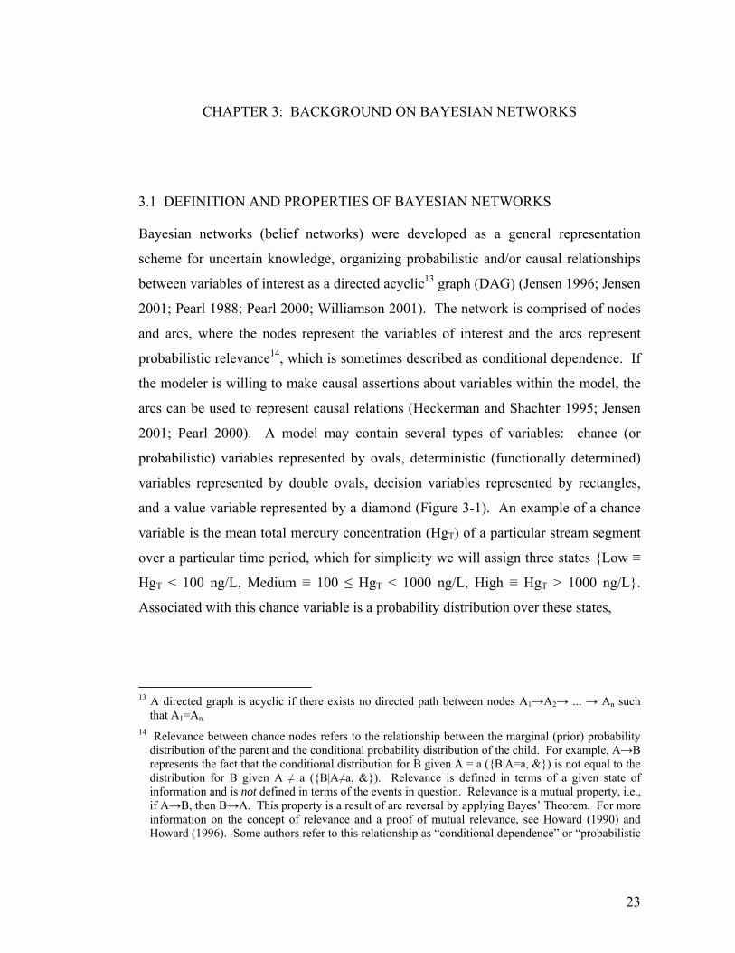
and a value variable represented by a diamond (Figure 3-1). An example of a chance

variable is the mean total mercury concentration (HgT) of a particular stream segment

over a particular time period, which for simplicity we will assign three states {Low ≡

HgT < 100 ng/L, Medium ≡ 100 ≤ HgT < 1000 ng/L, High ≡ HgT > 1000 ng/L}.

Associated with this chance variable is a probability distribution over these states,

13 A directed graph is acyclic if there exists no directed path between nodes A1→A2→ ... → An such

that A1=An.

14 Relevance between chance nodes refers to the relationship between the marginal (prior) probability distribution of the parent and the conditional probability distribution of the child. For example, A→B represents the fact that the conditional distribution for B given A = a ({B|A=a, &}) is not equal to the distribution for B given A ≠ a ({B|A≠a, &}). Relevance is defined in terms of a given state of information and is not defined in terms of the events in question. Relevance is a mutual property, i.e., if A→B, then B→A. This property is a result of arc reversal by applying Bayes’ Theorem. For more information on the concept of relevance and a proof of mutual relevance, see Howard (1990) and Howard (1996). Some authors refer to this relationship as “conditional dependence” or “probabilistic

24

Figure 3-1. Types of nodes in a Bayesian network for a decision situation.

perhaps conditioned on another variable. An example of a deterministic variable is the

HgT load at a particular point in time given the precise values of HgT and water flow,

since HgT load is functionally determined by these values. If there is uncertainty in the

state of the predicted HgT value for an observed (experimentally determined) flow,

then the deterministic variable HgT load will be represented by a probability

distribution over the possible load states, conditioned on HgT and flow. A

deterministic variable contains no uncertainty only if the states of its parents are

known with certainty. An example of a decision variable is a set of alternatives

{Alternative 1, Alternative 2, etc.}, exactly one of which will be chosen by a decision-

maker at some point in time. A value variable refers to a table of values (utilities)

associated with each of the possible outcomes for each alternative. A utility15

dependence”, e.g., Shachter (1986). When the arc is directed into a decision variable, the relationship may be termed “informational dependence” (Howard, 1990; Shachter, 1986; Pearl, 1988).

15 Utility may be defined in terms of lotteries. When examining a lottery, the decision-maker looks at the possible outcomes for the lottery, in which each outcome has an associated value (v) and a probability of occurrence (p). For example, assume that a two-outcome lottery (Lottery i ≡ Li) has outcomes A and B. The expected value of Lottery i is then computed as Li = pi,A*vi,A + pi,B*vi,B, where pi,j and vi,j refer to the probability and value (in dollars) of outcome “j” in Li. When comparing two lotteries, if the decision-maker prefers L1 to L2 (L1 ► L2), then a number u(Li) can be assigned to each lottery that describes the strength of the preference for that lottery. If these numbers are defined

25

represents the strength of the preference placed on that outcome by the decision-maker

(Luce and Raiffa 1989). See Chapter 4 for a discussion of using Bayesian networks

(influence diagrams) to evaluate alternatives and to perform decision analysis.

Probabilistic relevance between variables is quantified within the network by

conditional probability distributions for each variable given every possible

combination16 of values of its parent variables (Jensen, 2001). A variable with no

parents is quantified by an unconditional (or marginal) probability distribution. Arcs

into non-decision variables represent probabilistic relevance and arcs into decision

variables represent the relevant information available at the time the decision is made

(Howard 1990; Howard and Matheson 1984; Jensen 2001; Shachter 1986; Shachter

1988). The Bayesian network allows: 1) computation of the posterior probabilities of

any subset of the model variables given evidence about any other subset of model

variables; 2) determination of the most likely scenario that explains the observed

evidence; 3) determination of optimal decisions and value of information and control;

and 4) determination of the effects of intervention on variables on interest through

causal analysis, if causal assertions can be made (Jensen 2001; Pearl 1988; Pearl 2000;

Shachter 1986).

This last use of Bayesian networks is of particular interest for TMDL linkage

analysis. In other words, Bayesian networks may be used to make predictions about

the uncertain response of the natural system to changes in those variables over which

the decision-maker has some control. Bayesian networks without decision or value

nodes can also be used to model reasoning under uncertainty and may be used as

predictive tools in decision situations, e.g., water quality management decision

situations (Borsuk et al. 2001; Borsuk et al. 2003; Reckhow 1999; Stow and Borsuk

2003; Varis 1995). One of the advantages of using a Bayesian network approach is

over the set of lotteries such that u(L1) > u(L2) if and only if L1 ► L2, then a utility function u exists over the lotteries (Luce and Raiffa 1989, p. 29).

16 For simplicity of presentation, this discussion assumes that the model is based on discrete probability distributions.

26

that the model evolves as new information is collected, yielding an updated model that

reflects the current state of knowledge about the system of interest, synthesizing prior

information and new evidence using theoretically sound probabilistic calculus (Jensen

2001; Pearl 1988; Shachter 1988).

While Bayesian network models may be based on empirical probabilistic

knowledge of the system of interest, they can also be based on what is known about

the causal relationships between the variables of interest (Pearl 2000). The

introduction of expert knowledge about causal relationships between variables allows

natural system processes and behavior to be modeled using Bayesian networks. More

importantly, when that causality is only incompletely understood or data-limitations

exist, incomplete knowledge about causal relationships can be represented in terms of

causal relations between random variables and conditional probabilities that describe

these uncertain cause-and-effect relationships. Causal assertions made in Bayesian

networks, in effect, provide additional constraints on the flow of information through

the network when observations or interventions are made (Pearl 2000). When a

variable is observed to be in a particular state, the d-separation17 properties are

different from the situation in which the variable was placed in that state by an

intervention. These and other properties of causal networks are described in detail by

Pearl (2000). The importance of the decision context for defining causality is

described by Heckerman and Shachter (1995).

In the Bayesian network model of the Sulphur Creek mercury TMDL setting

decision situation, causal relations and conditional probabilities are based on what is

currently known about the relations between HgT sources, HgT loading, MeHg

production and the resulting loading, Hg fish-tissue burdens, and other natural-system

17 D-separation refers to the relationship between evidence introduction and evidence transmission for a

given model structure. Two variables are d-separated if, given the evidence entered into the network, no information (changes in belief) may pass between them. Jensen (2001) describes d-separated variables as “structurally independent” to emphasize the blocking of evidence between such variables. If two variables are not d-separated, they are said to be d-connected. The same two variables in a given model structure may be d-separated or d-connected depending on which variables in the structure receive evidence.

27

variables. The model also includes a probabilistic representation of what is currently

known about how mitigation efforts may impact the natural system. The composite

effect of predictive uncertainty and natural variability are represented as conditional

probability in these models.

Figure 3-2 shows two related examples of a Bayesian network representation

of a decision involving three uncertainties as chance nodes in which the arcs represent

causal relationships. The network in (a) of Figure 3-2 is completely generic and is

shown to illustrate different kinds of uncertain variables. As shown, this model says

that the states of Uncertain Variable 1, 2, and 3 will not be known before the decision

is made. In the case of Variable 2, its state is not influenced by the decision. The arc

from the decision to Uncertain Variable 1 means that while its state will not be known

before the decision, the probability distribution over Uncertain Variable 1 is

influenced by the choice of strategy. The path from the decision to Uncertain Variable

3 through the arc from Uncertain Variable 1 to Uncertain Variable 3 means that the

decision-maker also has some influence over its state. However, the arc from

Uncertain Variable 2 to Uncertain Variable 3 means that Uncertain Variable 3 will

also be influenced by something outside of the decision-maker’s control (namely

Uncertain Variable 2). In this way, uncertain decision-maker influence and

uncontrollable uncertainty can be coherently modeled in terms of the available

information and the best understanding of the causal behavior of the system being

modeled.

Note that the relationships between variables are the same in the causal

network shown in (b) of Figure 3-2. The same discussion from (a) holds, but we can

now think of these relationships in terms of meaningful variables. In this network, the

Load Allocation Decision (a decision about the strategy in reducing future total

mercury loadings) has some influence over the future state of “Mine HgT Loading”

(total mercury loading from some mercury mine source) over some time period, which

will influence the future state of “HgT Loading at Gage” (total mercury loading

downstream at a point of compliance) over the same time period. However, HgT

28

Loading at the Gage is also influenced by “Background HgT Loading” (total mercury

loading from all other sources upstream of the gage), which is not under the influence

of the decision-makers. In this context, the future state of Background HgT Loading

is highly uncertain.

In Bayesian network models, it is often useful to draw relevance relationships in

causal directions to increase the intuitiveness of the model (Heckerman and Shachter

1995; Pearl 2000). In this form, relationships between variables in Bayesian network

water quality models can be discussed in causal terms for the purposes of evidential

reasoning18, where this causal understanding may be based on knowledge of the

specific underlying causal processes involved or based on a statistical aggregation of

more complex associations (Reckhow 1999). However, it is emphasized that the

general definition of Bayesian networks does not refer to causality and that there is no

Figure 3-2. Bayesian Network Examples. (a) Generic decision involving three uncertain variables as chance nodes. (b) An analogous decision situation for managing mine-related total mercury loadings (Mine HgT Loading).

18 The task of evidential reasoning is to determine the validity of unobservable hypotheses from

observable evidence (Heckerman and Shachter 1995). The unobservable hypotheses are the variables of interest to the modeler, with the purpose being to estimate the probability that a particular hypothesis holds true given what has been observed.

29

requirement that arcs represent causal relationships. The definition of Bayesian

networks does, however, require that the d-separation properties implied by the model

structure hold for the system being modeled (Jensen 2001). It is often useful in

decision analysis to draw arcs in a causal direction for use by decision-makers, but to

reverse19 them for purposes of assessment or evaluation (Shachter 1988).

Causal relationships can be represented using Bayesian networks (Figure 3-3).

This figure shows a simple Bayesian network model relating stream flow, total

mercury loading, total aqueous mercury concentration, and total

(mono)methylmercury concentration in a stream segment over a specific time period.

This model asserts that total (unfiltered) methylmercury concentration (MeHgT) is

caused by total mercury concentration (HgT) and “other environmental factors”, which

may or may not have been observed. In turn, total mercury concentration in water is

caused by stream flow and total mercury loading. There are many physical, chemical,

and biological processes underlying these causal assertions, but the statements made in

this model are accurate based on current understanding (and perhaps even useful to

decision-makers, depending on the decision context).

19 Arc reversal is the application of Bayes’ theorem to a Bayesian network and implies appropriate

updating of the conditional probability distributions for the variables involved. The rules of and uses for arc reversal are described in, e.g., Howard and Matheson (1984), Shachter (1986), and Heckerman and Shachter (1995).

30

Figure 3-3. Graphical representation of a Bayesian network for relating mercury loading to methylmercury concentration.

To illustrate one of the points made explicit by the graph, MeHgT is conditionally

independent of stream flow (S) and total mercury loading (L) given the value of HgT

and the other relevant environmental factors (OF). This conditional independence is

represented graphically by the absence of arcs connecting stream flow and total

mercury loading to MeHgT, even though there is a path between them through the HgT

variable. It is emphasized that conditional independence in Bayesian networks refers

to the blocking of the transmission of evidence within the network and is not the same

as complete probabilistic independence (Jensen 2001; Shachter 1998). To illustrate, if

the value of total aqueous mercury concentration is not known, evidence concerning

total mercury loading (L) may be relevant to MeHgT.

The ability of Bayesian networks to incorporate conditional independence

greatly simplifies model development by allowing separate sub-models to be

31

developed for individual conditional relationships, where these sub-models may be

based on uncertainty analysis of a mechanistic model, statistical relationships in an

empirical model, or probabilistic information elicited from experts (Borsuk et al. 2001;

Borsuk et al. 2003). The Bayesian network itself represents a compact representation

of a particular factorization of the joint distribution over the model variables (Howard

and Matheson, 1984; Jensen, 2001). The factorization for the joint distribution over

the universe of variables for the model shown in Figure 3-3 is:

{S, L, HgT, OF, MeHgT} = Пi{i|Pa(i)} = {S|&}{L|S&}{HgT|S,L&}{OF|&}{MeHgT|HgT, OF,&},

where the product is over all of the model variables “i”, Pa(i) represents the set of

parents for variable “i”, and “&” designates the background state of information.

Chance variables can be further sub-divided into hypothesis variables (not

directly observable) and information variables, which may provide evidence that

reveals something useful about the hypothesis variables in the decision context (Jensen

2001). In the context of this decision problem, whether or not mine mitigation results

in a reduction in methylmercury concentration trends can be expressed as a hypothesis

variable or a set of related hypothesis variables. Total mercury concentration, reactive

mercury concentration in sediment, sulfate concentration, the distribution of

methylmercury concentrations throughout the watershed, etc., can then be modeled as

information variables that reveal something about the relevant hypotheses.

The variables included in an influence diagram model should fit one or more of

several criteria. They are either: 1) manageable, which means that the alternative

chosen influences its post-decision state (e.g., total mercury loads from a mine site); 2)

predictable from available data, models, or expertise; or 3) observable at the scale of

interest from the perspective of the water quality management problem. In addition,

chance variables are only included if they are: 1) of interest to the decision-makers

and/or stakeholders or; 2) helpful for assessing probability distributions for variables

that are of interest. These last two criteria could be summarized by the requirement

that a path exist between any chance variable and the value node. Another way of

32

saying this is that chance variables should be relevant to the value of the decision

outcome, if they are to be included in the influence diagram. 20

A Bayesian network that is completely represented graphically (all nodes and

arcs are present and correctly related), but that is missing some data, outcomes for

decision variables, or conditional probabilistic data for any of the variables is said to

be partially specified. If no data is missing, the network is said to be fully specified.

Partially specified network models are meaningful representations that carry

considerable information about the system being modeled. In fact, many predictive

and inferential queries can be fully answered from a partially specified model,

depending on the query, the model structure, and the required data (Shachter 1988).

3.2 LITERATURE ON RELEVANT APPLICATIONS OF BAYESIAN NETWORK

MODELS

There are two examples in the literature of a belief network approach being taken to

model regional water quality management situations: a series of papers regarding a

comprehensive study of nitrogen load reduction strategies for the Neuse River in

North Carolina (Borsuk et al. 2001; Borsuk et al. 2003; Reckhow 1999; Stow and

Borsuk 2003) and a application in the case of a phosphorus load reduction for the East

Canyon Creek in Utah (Ames 2002). The Neuse River work (Borsuk and others)

develops a Bayesian network model relating nitrogen loadings to algal densities,

eutrophication effects, and fish kills for several river segments. The purpose of the

model is to make predictions of future consequences of nitrogen load reductions on

these endpoints of interest to stakeholders. Stakeholder and decision-maker

preferences were not explicitly considered in the model.

20 An exception would be a variable or set of variables with no path to the value node, but that, for

whatever reason, are of interest to one or more decision participants.

33

3.3 SUMMARY

This chapter introduces Bayesian networks as a mathematical tool for modeling

uncertain causal relationships between variables of interest. It discusses several

important concepts needed for understanding Bayesian networks, including: 1) types

of variables; 2) the graphical notation for representing probabilistic relevance; 3) the

importance of causal assertions for environmental modeling with Bayesian networks;

4) d-separation, information “flow”, modularity, and the effects of evidence; 5) how

new information can be incorporated through belief updating; and 6) the uses of

Bayesian networks for making predictions and inferences and performing various

analyses. Other aspects of Bayesian networks are discussed in the context of decision

analysis (Chapter 4) and as the Bayesian network model of the Sulphur Creek mercury

TMDL is explicated in Chapters 5 and 6.

34

3.4 REFERENCES

Ames, D. P. (2002). "Bayesian Decision Networks for Watershed Management," Dissertation, Utah State University, Logan, Utah.

Borsuk, M. E., Clemen, R. T., Maguire, L. A., Reckhow, K. H., and Stow, C. A. (2001). "Stakeholder values and scientific modeling in the Neuse River watershed

A Bayesian network of eutrophication models for synthesis, prediction, and uncertainty analysis." Group Decision and Negotiation, 10, 355-373.

Borsuk, M. E., Stow, C. A., and Reckhow, K. H. (2003). "A Bayesian Network of Eutrophication Models for Synthesis, Prediction, and Uncertainty Analysis." Ecological Modelling, 173, 219-239.


Howard, R. A. (1990). "From Influence to Relevance to Knowledge." Influence Diagrams, Belief Nets and Decision Analysis, R. M. Oliver and J. Q. Smith, eds., John Wiley & Sons Ltd., 3-23.


Jensen, F. V. (1996). An Introduction to Bayesian Networks, UCL Press, London. Jensen, F. V. (2001). Bayesian Networks and Decision Graphs, Springer-Verlag, New

York. Luce, R. D., and Raiffa, H. (1989). Games and decisions : introduction and critical

survey, Dover Publications, New York. Pearl, J. (1988). Probabilistic Reasoning in Intelligent Systems: Networks of Plausible

Inference, Morgan Kaufmann Publishers, Inc., San Francisco. Pearl, J. (2000). Causality: Models, Reasoning, and Inference, Cambridge University

Press, Cambridge. Reckhow, K. H. (1999). "Water Quality Prediction and Probability Network Models."

Canadian Journal of Fisheries and Aquatic Sciences, 56, 1150-1158. Shachter, R. D. (1986). "Evaluating Influence Diagrams." Operations Research, 34(6),

871-882. Shachter, R. D. (1988). "Probabilistic Inference and Influence Diagrams." Operations

Research, 36(4), 589-604. Shachter, R. D. "Bayes-Ball: The Rational Pastime (for Determining Irrelevance and

Requisite Information in Belief Networks and Influence Diagrams)." San Francisco, 480-487.

Stow, C. A., and Borsuk, M. E. (2003). "Enhancing Causal Assessment of Estuarine Fishkills Using Graphical Models." Ecosystems, 6, 11-19.

Varis, O. (1995). "Belief Networks for Modelling and Assessment of Environmental Change." Environmetrics, 6, 439-444.

35

Williamson, J. (2001). "Foundations for Bayesian Networks." Foundations of Bayesianism, D. Corfield and J. Williamson, eds., Kluwer Academic Publishers, Dordrecht.

36

CHAPTER 4: A DECISION ANALYTICAL PERSPECTIVE ON TMDL

DEVELOPMENT

This chapter consists of a reviewed paper published as a conference proceedings paper

for the Water Environment Federation’s National TMDL Science and Policy 2003

Specialty Conference. The chapter describes the decision analytical framework built

upon in Chapters 5 through 8, but it takes a much more general view of preferences in

TMDL decision-making than the methodology actually used in these later chapters.

Some edits of the original paper were made for clarity and consistency with other

chapters in this dissertation.

37

A DECISION ANALYSIS APPROACH TO TMDL IMPLEMENTATION

DECISIONS: MERCURY TMDLS IN THE SAN FRANCISCO BAY AREA

William B. Labiosa1, 2, James O. Leckie1, Thomas Mumley3, James Rytuba4, and

Richard Bernknopf4

1. Department of Civil and Environmental Engineering, MC 4020,

Stanford University, Stanford, California USA 94305

2. Contact: [email protected]

3. California Regional Water Quality Control Board, San Francisco

Bay Region

4. US Geological Survey, Menlo Park, California, 94025

ABSTRACT

This paper describes a decision analysis approach to TMDL implementation decisions

for mercury using a mine-impacted tributary in the San Francisco Bay as an example.

Decision analysis is a demonstrably sound approach for making best decisions under

uncertainty (see, e.g., Howard 1968, 1988; Keeney and Raiffa 1976; Clemen 1996;

Merkhofer 1999). The Bayesian probabilistic nature of decision analysis makes it

ideal for integrating diverse information, including the results from scientific and

engineering models, cost and benefit models, empirical data, and expert judgment.

One significant advantage of a decision analysis approach is its explicit separation of a

decision problem into alternatives, information, and preferences. This, in theory,

allows decision-makers and stakeholders to separate “what we know” from “what we

want”. It is hypothesized that a more explicit separation of information and

values/preferences will focus the debate. While traditional decision analysis assumes

a single rational decision-maker (where “single” may also denote a group that agrees

on information and preferences), it can be extended to multiple decision-maker

situations in a variety of ways. Evaluating various extensions of decision analysis in a

38

TMDL implementation stakeholder context is one of the primary goals of this on-

going study. It is hypothesized that, in general, decision analysis provides a helpful

decision framework for a TMDL implementation planning/stakeholder process in

many circumstances.

KEYWORDS

Decision analysis, TMDLs, mercury, water quality predictions, influence diagrams,

Bayesian networks, probabilistic networks, information-gathering decisions, load

allocation decisions, mitigation decisions, sensitivity analysis, value of information

4.1 INTRODUCTION

BACKGROUND

There are a number of examples of the use of decision analysis for environmental

decision-making in the literature, often in the area of site selection or choosing

between remediation, restoration, or technology alternatives (e.g., Keeney 1980;

Merkhofer and Keeney 1987; Maguire and Boiney 1994; Reckhow 1994a; Merkhofer

et al. 1997; Perdek 1997; Kruber and Schoene 1998; Freeze and Gorelick 1999;

Merkhofer 1999; Bonano et al. 2000; Anderson and Hobbs 2001). Environmental

decision situations are often rife with uncertainty and controversy, requiring the

integration of diverse kinds of information and compromises between diverse

interests. TMDL load allocation decisions are typical in this regard (NRC 2001;

Boese 2002). Common TMDL decision issues include dealing with appreciable

scientific uncertainty and information gaps in understanding the relationships between

loadings, mitigation, and effects, determining whether to make allocation decisions

based on what is currently known or whether to collect new data and perform new

analyses before making those decisions, and prioritizing pre- and post-implementation

monitoring activities. Decision analysis provides a normative (as opposed to

39

descriptive) framework for providing decision clarity for these kinds of decision

problems. The theory behind decision analysis does not attempt to predict decision

strategies that people will choose, but rather, it attempts to predict decision strategies

people should choose, given a set of beliefs, alternatives, and preferences (the decision

basis). In a group decision situation, if consensus is achieved on the decision basis,

decision analysis can be used to determine optimal decisions. If consensus is not

achievable, decision analysis may be used to highlight areas of agreement and

disagreement, allowing insights into potential compromises and/or defining positions

for negotiation.

Decision analysis makes use of the Bayesian (subjective) definition of

probability, which treats uncertainty as a probability and allows the decision-maker to

combine various kinds of information into a unified probabilistic framework. For

decisions that involve perturbations to natural systems, Bayesian (probabilistic)

networks that are built up from the best available scientific models, data, and expert

judgments can be used to predict the consequences of those decisions (Borsuk et al.

2001, 2002; Stow et al. 2003; Reckhow et al. 1999). In practice, empirical stochastic

models, uncertainty analysis of semi-empirical models, and expert judgment are the

only feasible means to creating the needed probabilistic relationships. While rigorous

uncertainty analyses of large mechanistic models can be used for this purpose, the

computational burden is excessive (Reckhow 1999).

Bayesian (probabilistic) networks are designed to model the variables that are

of interest to decision-makers. Other variables that are useful for modeling the

variables of interest may be initially included, then eliminated using probabilistic

marginalization (Jensen 2001). In effect, the influences of hidden variables are

included in the conditional probability distributions of the variables in the model. The

cumulative effects of the many variables that may individually have a small effect on a

variable of interest are modeled as random “noise”, as well. This approach allows the

modeler to focus on predictive accuracy for the time and spatial scales desired for the

variables of interest to the decision-makers, removing details that are determined to be

40

extraneous to the decision problem. Again, the effects of these “details” are ideally

present in the conditional probability distributions of the modeled variables. As

pointed out by Reckhow (1999), this approach often leads to superior predictive

accuracy for the modeled variables compared to larger, more detailed deterministic

scientific models of water quality impacts. The loss of mechanistic descriptive power

is compensated by the ability to perform sensitivity analyses, explore scenarios

probabilistically, and estimate credibility of compliance predictions. Recent work has

demonstrated that water quality management effects can be effectively modeled using

Bayesian (probabilistic) networks (e.g., Reckhow 1999; Borsuk et al. 2001; Borsuk et

al. 2002; Stow et al. 2003). Since compliance is predicted probabilistically, a margin

of safety (MOS) can be explicitly considered in terms of credibility of compliance

predictions.

From a decision analysis perspective, the Bayesian network model of interest

is the influence diagram, which combines decisions (“what you can do”) with a model

of key uncertainties (“what you know”), subject to a valuation model (“what you care

about”) (Howard and Matheson 1984; Shachter 1986, 1988). If consensus is achieved

on preferences, influence diagrams allow determinations of optimal decisions,

sensitivity of the optimal decision to key uncertainties and assumptions, and value of

information on uncertainties, which may be used to plan future information-gathering

activities. Value of information refers to the fact that improvements in the state of

information before a decision is made can lead to a change in the predicted optimal

policy. It is the potential for changing the optimal policy that generates economic

value (see Howard 1968; Lawrence 1999).

Even without consensus on preferences, sensitivity analysis can be performed

to explore relationships between key uncertainties and variables of interest (e.g., water

quality endpoints), allowing the decision-makers to explore “what-if” scenarios of

interest. When preferences are ignored (i.e., the value model is removed), the

underlying Bayesian network may be referred to as a “belief network”. In the context

of water quality management decisions, belief networks can be thought of as modeling

41

the response of the natural system to management strategies. For example, one could

use a belief network to probabilistically explore the relationship between mercury load

reductions and fish tissue mercury levels under a variety of scenarios, in essence

demonstrating how beliefs about future fish tissue mercury levels change with load

reductions. This research project makes extensive use of influence diagrams and

belief networks as tools for performing TMDL decision analysis. However, the

emphasis is on the use of these tools for supporting decisions, not as water quality

models per se.

This paper demonstrates an influence diagram model of mitigation/load

allocation decisions for a simple mercury TMDL example. Such a model can be used

throughout the TMDL decision process, including initial information-gathering

decisions, load allocation/mitigation decisions, and post-implementation monitoring

decisions. The essential insight is that information-gathering/monitoring decisions,

whether made before or after allocation decisions, draw their value from making better

load allocation/mitigation decisions. For this reason, information-gathering decision

models build on load allocation/mitigation decision models. Our load

allocation/mitigation decision model integrates a Bayesian (probabilistic) network

model of environmental system response to mitigation decisions with a valuation

model, allowing insights into the credibility of compliance with multiple numerical

standards, insights into sensitivity of conclusions to small changes in model

parameters, and, if a value model can be defined, the determination of optimal

strategies.

It is emphasized that decision analysis applied to group decision situations

should be thought of as a process by which groups may discover useful insights that

highlight where consensus may be achieved and where obstacles requiring

clarification, negotiation, mediation, or litigation may lie. There are many competing

versions of decision analysis with variations on how alternatives are generated,

uncertainty is represented, preferences are elicited, etc. In this paper we describe a

decision analytic approach that is based on small group elicitation of goals, objectives,

42

and alternatives, a probabilistic model of natural system response, and several

potential methods for eliciting and representing preferences. Other related approaches

may be just as appropriate, depending on circumstances. One of the focuses of this

paper is dealing with the problem of competing preferences between stakeholders,

both from the perspectives of making decisions and representing preferences.

At the highest level, decision analysis divides the decision problem into

alternatives, information, and preferences. In the context of public environmental

decision-making, these could be cast as: 1) decision framing/strategy generation; 2)

information modeling/synthesis/forecasting; and 3) multiattribute utility analysis,

negotiation among interest groups, or other methods of eliciting and representing

preferences. Each of these aspects of decision analysis will be described further

through examples, with the goal of showing how decision analysis can create clarity in

a complex decision problem. But first, we discuss the importance of considering

uncertainty in the TMDL decision-making process.

UNCERTAINTY IN TMDL DECISIONS

Models play and will continue to play a central role in the TMDL development and

implementation process (Reckhow 1999; NRC 2001; Lung 2001; USEPA 2002).

Whether the models are empirical (statistical) or mechanistic, they represent the best

scientific understanding of how contaminant loadings relate to water body impairment

of designated beneficial uses (NRC 2001). Once a waterbody is listed as impaired,

predictive models are used to assess the relative contributions of various pollution

sources, to predict the total load reduction required to meet ambient water quality

standards, and to predict the relationships between specific control measures (e.g.,

point source load reductions) and water quality targets (e.g., ambient water

concentration of a particular pollutant) in the load allocation process.

Decision-making related to TMDL development and implementation requires

one to answer questions related to determining the reasons for non-attainment of

beneficial use and evaluating strategies for mitigating those determined causes.

43

Neither of these questions can be answered with certainty. Uncertainty, whether the

source is incomplete knowledge about the natural system, analytical error, or the

stochastic variability inherent in natural systems, is a reality that any water quality

management decision framework must recognize, assess, and, when possible, reduce

(NRC 2001). The decision analytic framework proposed in this paper specifically

addresses model uncertainty in the context of decision-making, using Bayesian

network models to integrate predictive uncertainty about the response of the natural

system to proposed mitigation strategies with stakeholder valuations of the strategies

being considered.

Uncertainty in model predictions can be large and, when explicitly considered,

can confound interpretation of results in terms of the decisions that need to be made

(Reckhow 1994b). Uncertainty has been, however, often treated superficially in water

quality management decisions, which can be a major source of contention between

stakeholders and regulatory agencies (Ortolano 1997; NRC 2001). Historically, this

occurred because the ability to analyze uncertainty was limited by computing power

and, in some cases, by a lack of understanding of how to feasibly model and propagate

uncertainty in large mechanistic water quality models. Besides the technical aspects,

even when uncertainty analysis is performed well, the political reality is that

discussions of the estimated uncertainty often get bogged down with arguments that

have more to do with preferences than information. In fact, the use of decision

analysis is an attempt to incorporate uncertainty directly into TMDL modeling and

decision-making in a manner that separates information and preferences. In effect,

this attempts to separate the estimation of uncertainty from the interpretation of

uncertainty. Disagreements about particular beliefs and preferences can be expected

to remain, but decision analysis may be able to focus the argument on those sources of

disagreement, reducing confusion about the impact of uncertainty on decisions.

Downplaying uncertainty to avoid these confrontations may make for an easier

stakeholder process in the short term, but that strategy runs of the risk of resulting in

poorly informed decisions. The National Research Council (ibid.) suggests the use of

adaptive management to deal with the significant uncertainty involved in TMDL

44

decisions, an approach that is being employed in many TMDLs. As discussed by

Reckhow et al. (2002), an adaptive management approach may be modeled with

Bayesian networks, but further discussion of adaptive management is beyond the

scope of this paper.

PREFERENCES

If decision outcomes can be valued in terms of a single attribute (e.g., an exchangeable

resource like dollars), and consensus can be reached regarding those values and

attitudes toward risk, decision analysis can be applied straightforwardly to determine

an optimal decision policy, sensitivity analysis can be used to determine the value of

information, etc. (e.g., Howard 1968; 1988; Marshall and Oliver 1995; Clemen 1996;

Merkhofer 1999). The optimal decision policy for an uncertain decision situation is

the policy that maximizes expected utility, a measure of value. By making maximum

expected utility the decision criterion, the utility of a particular outcome is weighted

by its probability of occurrence, so that the strategy that yields the highest expected

utility can be thought of as promising the “highest probability of achieving the best

outcome”.

When a group agrees to cooperate and work towards consensus on information

beliefs and preferences, the single decision-maker decision analysis approach may be

used. Single decision-maker problems involving utility over uncertain monetary

outcomes are solved in terms of expected utilities, incorporating risk attitudes. Non-

monetary outcomes can be accommodated in decision analysis using the “preference

probability” interpretation of utility, in which the utility of an outcome is interpreted

as the probability of obtaining the best outcome instead of the worst outcome. The

approach we explore in this paper is the use of multiattribute utility analysis to directly

define a mapping from either monetary or non-monetary outcomes to utilities (Howard

1984b; Marshall and Oliver 1995; Clemen 1996; Lawrence 1999).

However, the assumptions applying in single decision-maker situations

obviously would not describe many TMDL decision situations, which instead can be

45

expected to have multiple goals with multiple associated attributes with perhaps no

obvious consensus on valuing the various possible outcomes. Note that there are two

important issues at stake here: 1) TMDL goals have multiple attributes that may not be

expressible in terms of a single measure like dollars; and 2) based on experience, we

can expect disagreements between work group/stakeholder group members about

valuing outcomes even within an agreed-upon multiattribute framework. Each of

these issues can be dealt with, if the TMDL decision-making group is willing to

cooperate. This does not require that consensus in preferences is achieved, but it does

require that group members agree to faithfully participate in the decision analysis

process.

Work groups and stakeholder groups may use decision analysis in a number of

ways, including a “competing models” approach in which the work group/stakeholder

group partitions into sub-groups that agree to act cooperatively in determining mutual

preferences and preferred alternatives for the purpose of arriving at negotiating

positions for each sub-group (Chechile 1991). In other words, the sub-groups agree to

effectively behave as a “single decision-maker” to determine recommended strategies

according to the sub-group’s viewpoint. While major differences may be found

between the various recommended approaches, numerous points of agreement are

expected. At this point, decision analysis may be used further with mediated

compromises on preferences and information that allows a group “best compromise

strategy” to be formulated, but it may be necessary to resort to a purely negotiated or

political compromise at this point. The advantage of applying decision analysis in this

latter case is that the sources of disagreement can be more easily identified and that

potential compromises may become more apparent. However, if a sub-group is non-

cooperative and misrepresents their beliefs and preferences in the analysis, decision

analysis may not be a useful tool for the TMDL decision-making process. Note that

other analytical approaches are similarly hobbled by deliberate attempts to

misrepresent positions (e.g., cost-benefit analysis). In such cases, political solutions

may be inevitable. In cases in which group members are willing to cooperatively state

46

their beliefs and preferences, decision analysis is a robust process that should be

considered.

DECISION ANALYSIS PROCESS

Figure 4-1 shows a flow diagram representing the decision analysis cycle (Howard

1984a). In a real application of decision analysis, individual steps may be emphasized

or de-emphasized, depending on the particular situation. Also, a particular step may

be accomplished using very different tools and some tools may be used in more than

one step. So, from a “tools perspective”, two different decision analysis applications

may appear to be very different, so much so that it may be difficult to see the

relationships between the two approaches. However, taking a decision analysis cycle

perspective, one can see how the seemingly different approaches accomplish the basic

steps in decision analysis. For the purposes of this paper, we will focus on 1) decision

framing/structuring; 2) probabilistic modeling of the natural system response; 3)

sensitivity analyses; and 4) dealing with preferences and potentially determining

optimal strategies and value of information. In particular, we will explore the

application of decision analysis to load allocation/mitigation decisions and

information-gathering decisions.

47

Figure 4-1. Decision Analysis cycle.

Structure Decision Problem:Identify decision situation, explore andidentify objectives, identify alternatives

Deterministic Analysis:Deterministic model of decision problem;Deterministic sensitivity analysis (tornadodiagram) to identify important uncertainties

Probabilistic Analysis:Probabilistic model of decision problem;Determine best strategy; Performsensitivity analyses

Appraisal:Value of information; Decision qualitydiagram; Is further analysis needed?

Commitment to Action

Initial Situation

48

The initial step in the decision analysis cycle is preliminary framing and

structuring of the decision situation in such a way that decision analysis may be used

to evaluate the various alternatives. In particular, framing involves identifying and

discussing decision performance measures, e.g., decision objectives and their

associated measurable/ predictable attributes. Performance measures (attributes) can

be thought of as gauging the consequences that the decision-maker cares about, so that

the range of possible outcomes may be represented in a meaningful way (Keeney

1992).

The influence diagram (as a Bayesian network) is a powerful tool that allows

the decision analyst to perform the deterministic analysis phase, the probabilistic

analysis phase, and, if a value model can be determined, to estimate the value of

information on key uncertainties and assumptions. In brief, the deterministic analysis

phase translates the results of the framing analysis into a mathematical model for the

purpose of determining which uncertainties are important enough to warrant

probabilistic modeling in the subsequent probabilistic analysis phase. The

probabilistic analysis phase assigns probabilities to the identified key uncertain

variables. Input variables that have little effect on the value model output are assigned

nominal (base) values and, thus, are treated deterministically. The required

probability distributions are either modeled empirically from data or assessed from

experts and/or decision-makers. In some cases, it may be advantageous to

probabilistically combine empirical models with expert opinion. In the probabilistic

analysis phase, optimal decisions may be determined if a value model can be

constructed. The influence diagram may be further manipulated to perform

probabilistic sensitivity analysis to determine how sensitive the optimal policy is to

current beliefs about key uncertainties. The decision analyst may find that the optimal

policy may change given small changes in probability distributions for a key

uncertainty, in which case further analysis may be recommended. Performing and

reporting the results of sensitivity analysis may be critical in achieving the degree of

“decision transparency” that promotes buy-in from stakeholders.

49

Value of information analysis may also be performed as this stage to determine

if additional information may have the potential to change the optimal policy. From a

decision analysis perspective, new information only has value when the optimal policy

may change in response to the new information (Howard 1968; Lawrence 1999).

Since value of information analysis requires consensus in preferences, it may not

resolve disagreements about information-gathering or technical review activities

between sub-groups. However, it can provide the basis for positions on information-

gathering and technical review activities within sub-groups and can shed light on the

sources of agreement and disagreement regarding these activities.

INFLUENCE DIAGRAMS (BAYESIAN NETWORKS) FOR ENVIRONMENTAL DECISION

ANALYSIS: GRAPHICAL TOOLS FOR DECISION PROBLEM FRAMING

Influence diagrams are often used as framing tools for graphically representing the

decision problem in terms of the relationships between decisions, uncertainties, and

performance measures (Howard and Matheson 1984; Shachter 1988; Howard 1990;

Merkhofer 1990; Marshall and Oliver 1995). The influence diagram can be

constructed as a group exercise in decision framing, focusing attention on the

relationships between the important variables in the decision situation, including

decision strategies, uncertain variables describing the state and response of the natural

system, and variables related to valuing outcomes. In addition to graphically

representing important aspects of the decision problem, the influence diagram can be

used to determine information/ forecasting requirements, probability assessment order,

and, if decision trees are to be used, decision tree structure. Deterministic sensitivity

analysis may later determine that one or more uncertainties can be treated

deterministically and hence the influence diagram may evolve during the decision

analysis problem. The role of the influence diagram in determining information and

modeling/forecasting needs is very important: this approach helps decision-makers

and technical experts/scientists communicate about what information is important in

terms of the decisions to be made.

50

INFLUENCE DIAGRAMS AS BAYESIAN NETWORKS FOR SOLVING DECISION PROBLEMS

In addition to decision framing, influence diagrams can also be used directly as

Bayesian network models by adding to the graph the requisite probability structures

needed for modeling consequences and value. In this use, an influence diagram is a

class of Bayesian networks that may include nodes representing uncertain system

variables, deterministic system variables, decision variables, and a value variable.

Optimal decisions are those that maximize expected utility through relationships

between the value variable and the other variables. Thus, influence diagrams can be

used in lieu of or in parallel with decision trees to solve for optimal decisions, to

evaluate sensitivity of the optimal decision to information and model assumptions, to

estimate the value of information and control, and to make inferences from the

available data important to the decision situation (Howard and Matheson 1984;

Shachter 1986; Oliver and Smith 1990; Pearl et al. 1990). In the approach described

in this paper, decision trees (Chechile 1991; Marshall and Oliver 1995) are avoided

altogether and the Bayesian network is used as the primary analytical tool.

To emphasize the point, the Bayesian network version of the influence diagram

may be used to make predictions about the response of the natural system to changes

in those variables over which the decision-maker has some control. Bayesian

networks without decision or value nodes (“belief networks”) can be also used to

model reasoning under uncertainty and may be used as predictive tools in decision

situations, e.g., water quality management decision situations (Reckhow 1999; Borsuk

et al. 2001). One of the advantages of using a Bayesian network approach is that the

model evolves as new information is collected, yielding an updated model that reflects

the current state of knowledge about the system of interest, synthesizing prior

information and new evidence using theoretically sound probabilistic calculus (Jensen

2001; Shachter 1986, 1988; Reckhow 1999; Pearl et al. 1990; Varis 1995).

Figure 4-2 shows an example of a Bayesian (belief) network representing

causal relationships between precipitation, creek flow, river flow, mine mercury load,

creek mercury load, and total mercury in water (HgT). The belief network consists of

51

a graph and probabilistic data associated with the nodes in the graph. The graph

consists of nodes (ovals) connected by arrows. Ovals represent chance (uncertain)

nodes and associated with each chance node is a random variable. The random

variables in the Bayesian network represent the attributes of interest to decision-

makers. Arrows represent potential conditional probabilistic dependence between the

various random variables and can be drawn in a causal direction. Graphically, the

arrow points from the “parent node” to the “child node”, which intuitively indicates

that the child node somehow “depends” on the parent node. More precisely, an arrow

from a parent node to an uncertain variable (child) means that the probability

distribution in the uncertain variable (child) is conditioned on the state of the parent

node. The absence of an arrow between two variables indicates that the variables are

conditionally independent. If there is a directed path between two variables (i.e., there

exists a set of arcs between them which can be traversed in the direction of the arcs)

which do not have a direct parent/child relationship, those variables may or may not be

relevant to one another, depending on the state of information. For example, Figure 4-

2 asserts that precipitation may be relevant to total mercury in water (HgT) if at least

one of the values for “Mine Hg Load”, “Creek Hg Load”, and “River Flow” has not

been observed. But, it also asserts that, given observations for “Mine Hg Load”,

“Creek Hg Load”, and “River Flow”, precipitation and total mercury in water are

conditionally independent of each other. These assertions of conditional independence

are very important in terms of understanding information needs and performing

decision analysis.

The variables included in a network may be included for a variety of reasons,

including the decision-makers’ direct interest in the state of a variable (e.g., HgT) or

because the variable helps to interpret or predict those variables of direct interest (e.g.,

precipitation). It is important to understand that variables needed from a technical

perspective for modeling a particular complex system do not need to be shown in the

version of the Bayesian network used for decision analysis, communicating with

decision-makers or stakeholders, etc. Variables needed only for modeling reasons can

be probabilistically absorbed into the network, which yields the same results as before

52

the nodes were removed. The local representation is changed, but the global

probabilistic relationships are not affected (Shachter 1988; Pearl et al. 1990). As there

may indeed be variables of interest to scientists about the natural system being

modeled that are not important to decision-makers, this is an important point to

understand.

The conditional probabilistic relationships between conditionally dependent

variables can be quantified in a modular fashion using an approach suitable to the kind

and amount of information available, where this modularity follows from the

conditional independence relationships in the model (Reckhow 1999, 2002). This

allows various kinds of statistical and subjective probabilistic information (from data,

models, and expert judgment) to be integrated into a single probabilistic network

model that can be used for predictions and inferences of use in decision-making

situations. Prediction refers to following an arrow in the forward direction, i.e.,

predicting the probability distribution of a child node based on the values or

distributions of its parent nodes. Inference refers to following an arrow in the reverse

direction, i.e., inferring the probability distribution of the parent nodes based on

evidence about the value of the child node(s) (Jensen 2001). The ability of a Bayesian

network to make predictions is useful,

53

Figure 4-2. An example of a Bayesian network.

Precipitation

Mine Hg Load

Creek Flow

Creek Hg Load

River Flow

HgT in water

for example, when trying to model the effects of particular mitigation strategies on

water quality attributes of interest. Learning what new evidence about a predicted

variable means in terms of hypotheses about cause and effect between parent and child

nodes is an example where the ability of Bayesian networks to perform inference may

be useful.

A point that needs to be emphasized here is that while such an influence

diagram model (or any other model) is an imperfect representation of the real system,

it should faithfully represent how the decision-maker believes the real system will

behave, given the available data and current scientific understanding. The decision-

maker can do no better than this when making a decision. In particular, if the optimal

strategy is sensitive to slight changes in the underlying probability distributions, then a

value of information analysis may determine that re-framing the load

allocation/mitigation decision problem as an information-gathering decision problem

may be the best course of action. If there are regulatory constraints that prevent this

re-framing, using the existing model to suggest optimal strategies is the best course of

action, from the decision analytical perspective.

54

4.2 METHODOLOGY AND DISCUSSION

FRAMING THE DECISION: OBJECTIVES HIERARCHY

Decision framing tools are used to represent the decision situation in a way that

enables the evaluation and comparison of alternatives according to criteria that are

meaningful to the decision-maker. The objectives hierarchy is a common framing tool

that identifies and organizes decision outcome performance measures (attributes),

which are used as evaluation criteria (Keeney 1992) and can be used as variables in an

influence diagram representation of the decision problem. Keeney (ibid.) organizes

the objectives hierarchy with: 1) an overarching decision goal at the top of the

hierarchy; 2) a set of issue-specific objectives consistent with and subject to this top

goal; and 3) a set of attributes consistent with and subject to the specific objectives.

There may be more than one level of objectives between the top decision goal and the

decision attributes, depending on the framing desired by the decision-makers.

Attributes are ideally the performance measures that the decision-makers care about,

and they should be chosen to be well-defined, measurable (at least in theory) and

predictable. When the objectives hierarchy is complete, the attribute set formed

should be comprehensive (capture all of the aspects of value at stake), minimal (as

small in number as possible), independent of one another, and operationally feasible

(Keeney and Raiffa 1976; Reckhow 1994a). These requirements ensure that there are

no “holes” or “double-counting” in the analysis and that a suitable value model can be

constructed (Merkhofer 1999).

Figure 4-3 shows a hypothetical objectives hierarchy for a mercury TMDL for

a tributary to the south San Francisco Bay. In practice, the objectives hierarchy would

be developed by the TMDL work group and/or stakeholder group, with the help of the

decision analyst. The top goal in this example objectives hierarchy is to manage

mercury contamination in the watershed, with objectives pertaining to protecting

human health and wildlife (sub-objectives of reducing mercury methylation potential

and methylmercury levels), meeting Basin Plan water quality objectives for total

mercury, maintaining adequate flood control, meeting the ten and twenty year total

55

mercury load reductions under the San Francisco Bay mercury TMDL, and controlling

compliance costs. Each objective is translated into one or more attributes, and this is

shown graphically by arrows pointing from a given objective to its attributes

(performance measures). Attributes serve multiple roles in decision analysis. They

form the basis of the value model, since they are the performance measures that matter

to decision-makers, and they define information needs for decision modeling. In this

latter role, TMDL decision situation attributes help define which natural system

variables need to be modeled for relating management strategies to value, as will be

demonstrated below.

For example, the “fish tissue mercury levels” attribute might be defined as the

average fish tissue mercury burden of a particular fish species (with perhaps specified

weight range, sex, etc.) within the watershed over some time scale. An attribute that

might be less obvious in the context of mercury mitigation, but that may be very

important to some stakeholders is flood capacity. The use of flood capacity as an

attribute allows decision-makers to keep track of the impact of mitigation strategies on

flood capacity, while simultaneously evaluating those strategies in terms of other

attributes. While establishing TMDL performance measures is an explicit activity in

the TMDL process, it is important to identify a list attributes that capture all

stakeholder values that may be significantly affected. To emphasize the point, it is

important to frame the problem not just in terms of “technical TMDL endpoints”, but

also in terms of attributes that characterize objectives that matter to stakeholders in

terms of idiosyncratic preferences. In fact, capturing this latter class of attributes may

make the difference between understanding why stakeholder values lead to

disagreements about acceptable strategies later in the decision process and finding a

situation in which there are arguments that are seemingly about “technical

information”, but that really reflect unstated preferences.

56

Figure 4-3. Hypothetical objectives hierarchy for managing mercury in a small mine-impacted tributary to the South Bay.

Manage Mercury Contamination in the Watershed in Terms of Objectives for Water Quality, Flood

Control, and Human and Ecological Health

Control Costs

MitigationCosts

CostDistribution

InformationGathering

Costs

Protect Human Health andWildlife

MeHgPotential

MeHgT

Control HgLoads to South

SF Bay

MeHgT Loadto South Bay

HgT Loadto South

BayShading

ArealExtent

MaintainFlood Control

Flood ControlModification

Costs

FloodCapacity

Meet Basin Plan Objectivesand Attain Federal Water

Quality Standards

HgT

Hg FishTissueLevels

FloodControlBenefits

ReduceMeHgLevels

DissolvedOxygenLevels

Reduce MeHgPotential

Sulfate

It is common, but often unheeded, advice in the decision analysis literature to

appropriately focus attention at this step since careless framing can lead to “solving

the wrong problem”, leading to inappropriate or incomplete consideration of

alternatives, a short-sighted understanding of the decision situation, and a

misappropriation of resources (Howard 1968; 1988; Reckhow 1994a; Clemen 1996;

Merkhofer 1999). Nevertheless, decision-makers often treat this stage cursorily and

plunge quickly into more familiar territory: technical problem framing, information-

gathering, modeling, and analysis. Decision-makers often have a good understanding

of many aspects of the decision problem “going in” to a particular decision situation,

which can sometimes lead to the misapprehension that detailed decision framing

exercises are unneeded. However, extensive decision framing can lead to better

planning and resource allocation and to evaluating the “right alternatives” in terms of

57

the “right attributes” for making good TMDL decisions. To a significant degree,

TMDL guidance documents already promote this activity from the technical

perspective.

IDENTIFYING ALTERNATIVES AND GENERATING STRATEGIES

Keeney (1992) describes a number of methods for using the attributes and objectives

from the objectives hierarchy to explore and generate decision alternatives. Clemen

(1996) provides a basic and useful summary of various techniques, including some of

the methods discussed in Keeney (ibid). The methods build on the identified goals,

objectives, and attributes, stressing the importance of flexibility and creativity. One

tool in particular may be useful for generating TMDL strategies: the strategy table.

Figure 4-4 shows a simple example of a strategy table with two strategies. Strategy

tables are fairly intuitive and the tool can be used in a group setting without much

introductory material required. The basic idea is to capture the possibilities, then to

select a manageable number of strategies as alternatives for further decision analysis.

A strategy consists of a set of single elements from each column in which the

combination of those elements makes sense as an approach. There will, of course, be

combinations that are incoherent and these combinations would not represent a viable

strategy. In a real TMDL allocation decision situation, the strategy table would be

expected to have more elements (columns), making such an approach useful for

brainstorming and organizing complexity. In Figure 4-4, two strategies are shown for

illustration: 1) a methylmercury potential mitigation strategy that includes “medium

reductions” for mine site and creek mercury loads and an aggressive reduction of

mercury methylation potential and 2) a mine site mercury load reduction strategy that

includes a large reduction requirement for mine site mercury loading and minimal

reductions for creek mercury loading and mercury methylation potential.

Once an objectives hierarchy has been created and alternatives have been

generated, the decision analyst will work with the group to create an influence

58

diagram from the chosen attributes, alternatives, and variables representing identified

important

Figure 4-4. Strategy table example.

MeHgMeHg Potential Potential Mitigation Mitigation FocusFocus

Medium Medium ReductionReduction

Medium Medium ReductionReduction

Strategies Mine Site Hg Load Allocation

Creek Hg Load Allocation

MeHg Potential Mitigation

Small Reduction

Small Small ReductionReduction

Small ReductionSmall Reduction

Medium Reduction

Large Large ReductionReduction

Large Reduction

Large ReductionLarge Reduction

Strategies Mine Site Hg Load Allocation


MeHg Potential Mitigation

Small Reduction

Small Small ReductionReduction


Medium Reduction

Large Large ReductionReduction

Large Reduction


StrategiesStrategies Mine Site Hg Load Allocation

Mine Site Hg Load Allocation



MeHg Potential MitigationMeHg Potential Mitigation


Small Small ReductionReductionSmall Small ReductionReduction

Small ReductionSmall ReductionSmall ReductionSmall Reduction

Medium ReductionMedium Reduction

Large Large ReductionReductionLarge Large ReductionReduction


Large ReductionLarge ReductionLarge ReductionLarge Reduction

Mine Site Load Mine Site Load Reduction FocusReduction Focus

uncertainties. Attributes may become variables in an influence diagram or may

become part of the value model, depending the nature of the attribute. It may be

worthwhile to revisit the objectives hierarchy and strategy table after the influence

diagram has been created to see if revisions are necessary.

MULTIATTRIBUTE UTILITY ANALYSIS

Multiattribute utility analysis (MUA) is designed to deal with the complexity of

eliciting and representing the values at stake in complex decision problems like

environmental decision situations (Keeney and Raiffa 1976; Gregory 1999; Merkhofer

1999; Prato 2003). In particular, multiattribute utility analysis (MUA) or other

59

approaches (e.g, the analytic hierarchy process) may be used to elicit and represent

preferences when multiple decision attributes/criteria are important (Chechile 1991;

Marshall and Oliver 1995; Merkhofer 1999). In general, MUA is conceptually simple,

but may become operationally complex with details that should burden the decision

analyst and not the decision-makers/work group. One problem is that lay people may

see this apparent complexity as being suspect, so great care should be taken to ensure

that decision-makers/work group members sufficiently understand the concepts being

used so that the preference representation approach is trusted (Morgan and Henrion

1990).

While there may be consensus that one alternative appears superior to the

others in terms of one particular attribute, it may appear inferior in terms other

attributes. Trade-offs between attributes is thus usually necessary and this idea is at

the core of multiattribute decision-making (Keeney and Raiffa 1976; MacCrimmon

and Wehrung 1977; Merkhofer et al. 1997). MUA can be used directly to rank

alternatives in terms of weighted utilities (Prato 2003), ignoring probabilities of

outcomes in the decision-making process. However, it can also be used in a decision

analysis framework that includes a probabilistic treatment of uncertainty and that

determines best policies based on expected utility.

Once the decision analyst elicits preferences between outcomes among the

various decision attributes for each decision-maker sub-group, the consensus

preferences for each sub-group can be aggregated into a multiple-attribute utility

function and maximum expected utility can be determined. Note that MUA does not

require monetization of preferences, one of the appeals of the technique. Other

approaches like probabilistic cost-benefit analysis, cost-effectiveness analysis,

minimization of chance of worst possible outcome, etc. could also be used, depending

on the situation (Morgan and Henrion 1990).

To illustrate the MUA process, Table 4-1 shows an example multiattribute

utility analysis (MUA) for a few outcomes for the two strategies from Figure 4-4,

60

MeHg Potential mitigation focus (Strategy 1) and mine site Hg load reduction focus

(Strategy 2), as evaluated by a hypothetical decision-maker sub-group. Other sub-

groups could be expected to have different results. This analysis assumes that the

decision problem is being modeled with discrete probabilities and that there are a

finite number of possible outcomes. MUA can then be used to elicit a utility function

from the decision-makers over those outcomes, as suggested by this example. Here

the sub-group chose a weighting scheme of 0.3 for cost, 0.6 for credibility of

compliance with total mercury load to the South Bay target, and 1.0 for credibility of

compliance with fish tissue mercury level target. Composite utilities are shown in the

rightmost column. Other approaches to defining a multiattribute utility function or

analogous scoring functions could be used, depending on the wishes of the subgroup.

Credibility of compliance refers to the conditional probability (not

“confidence” in the statistical sense) that a particular attribute has a value that meets a

particular target (threshold) value, as computed within the network. The threshold

could itself be uncertain, but need not be. The credibility of compliance in essence

becomes a node in the Bayesian network conditioned on the attribute (target) of

interest. The concept is similar to the “confidence of compliance” described in the

literature, but is referred to here as a “credibility” since it is not statistical confidence

to which we are referring. The concept may prove to be useful for evaluating

mitigation/allocation strategies since strategies that yield higher probabilities of

success would naturally be more appealing.

While the sub-groups may well arrive at different conclusions, their respective

positions should be well-defined in terms of beliefs about probabilities of outcomes

and their preferences. Consensus building exercises that attempt to arrive at

compromises may be performed or negotiation between the various sub-groups may

follow. Again, the advantage of using decision analysis is that the positions of each

sub-group should be clear and the various sources of differences in positions should be

apparent. The price that must be paid to get to this point is that the work group

members must agree to accurately state their beliefs and preferences. If trust is

61

lacking, then appropriate measures may be required (e.g., allowing sub-groups to

develop their positions privately without sharing analyses) or non-analytical

approaches may be required. Exploring the

Table 4-1. Multiattribute utility analysis for several outcomes for strategies 1 and 2 for a particular sub-group.

Possible Outcomes Utility

on Cost1Utility on

COC Load2

Utility on COC fish3

Composite Utility Using Weighting

SchemeStrategy 1, Cost = 15, COC Load = 30%, COC fish = %20

10 2 1 5.2

Strategy 1, Cost = 30, COC Load = 35%, COC fish = 50%

6 3 9 12.6


6 4 4 8.2


2 8 6 11.4

.... other outcomes ... ... ... ... Notes: 1) Mitigation cost 2) Credibility of compliance with total mercury load to the South Bay target 3) Credibility of compliance with fish tissue mercury level target

62

possibilities and determining “what works and why” is an active area of research in

the field of collaborative group decision-making .

Such a multiattribute utility function could be used in an influence diagram

model of TMDL decisions to determine optimal decisions, perform sensitivity analysis

for expected utility, and estimate the value of information in terms of utility. If

preferences can be expressed in monetary terms, a monetary value of information can

be estimated for the uncertainties. One could argue whether or not this is appropriate,

but the choice reflects the wishes of the sub-group cooperating in the analysis.

Whether the scale is dollars or utility, value of information provides a useful signal for

prioritizing information-gathering activities and technical review needs.

INFLUENCE DIAGRAMS FOR FORECASTING ALLOCATION DECISION CONSEQUENCES

Designing and implementing a Bayesian network model occurs in three stages: 1)

development of the graphical model linking the identified variables in terms of

conditional independence relationships; 2) assessment of the required conditional or

marginal probability distributions for each variable; 3) entering evidence/observed

data (if applicable) on observable nodes in the compiled model to see how beliefs in

unobserved nodes are affected (Jensen 2001). In the example that follows, the

Netica™ Application for Belief Networks and Influence Diagrams (Norwys Software

Corp. 1996) was used to implement the model. Other Bayesian network development

environments include the MatLab Bayes Net Toolbox (Murphy 2002), the GeNIe©

software package (University of Pittsburgh), Microsoft® Bayes Networks (MSBN),

and Analytica® (Lumina Decision Systems, Inc.). Russell Almond at the University

of Washington maintains a website listing and reviewing Bayesian network software:

http://www.stat.washington.edu/bayes/almond/belief.html#MSBN. Morgan and

Henrion (1990) discuss considerations and issues in choosing a computing

environment for probabilistic analysis.

Figure 4-5 shows an influence diagram that describes a decision situation

building on the belief network from Figure 4-2. This influence diagram includes a

63

decision variable (Load Allocation/Mitigation Decisions), new chance variables for

mercury methylation potential, total mercury in water (MeHgT), fish tissue mercury

levels, annual total mercury load to the Bay, mitigation cost, credibility of compliance

(discussed below) for methyl mercury levels in fish, and, credibility of compliance for

total mercury load to the Bay. It also includes a multiattribute utility node (value

node) defined in terms of mitigation cost, credibility of compliance with a mercury

fish tissue target, and credibility of compliance with the annual total load to the Bay

target. By eliciting decision-maker (sub-group) preferences over outcomes in terms of

these three attributes with multiattribute utility analysis, optimal load

allocation/mitigation decisions can be determined for the sub-group using this model.

64

Figure 4-5. Influence diagram for mercury load allocation/mitigation decisions for a small watershed impacted by a mercury mine site and mine wastes.

Multiattribute Utility

Mine Hg Load

HgT in water

Creek Hg Load

MeHgT in water

Hg Methylation Potential

Hg Fish Tissue Levels

Mitigation Cost

Credibility of Compliance

Annual HgT Load to Bay

Credibility of Compliance

River Flow

Creek Flow Load Allocation/Mitigation Decisions

Precipitation

Key:

Chance Node

Value Node

Decision Node

65

The influence diagram in Figure 4-5 states that, given the total mercury

concentration in water (HgT) and river flow, the annual total mercury load to the South

Bay is independent of the mine and creek loads. Precipitation is modeled using a

marginal (unconditional) distribution based on the available historical data and creek

flow is modeled conditioned on precipitation. The mine mercury load is modeled as

being conditional upon precipitation and the mine site mercury load allocation. The

creek mercury load is modeled as being conditional upon creek flow and the creek

mercury load allocation. To further illustrate the concept of conditional independence,

note that given observations for HgT and river flow (e.g., annual average values over

the waterbody), the annual total mercury load to the South Bay is conditionally

independent of the creek Hg load and mine site Hg load. This does not mean that

creek Hg load and mine site Hg load do not impact the total annual Hg load to the

Bay, but rather that the influence is through the HgT variable. From a causal

perspective, the observed HgT value would “reflect” any influence from the mine site

and creek Hg loadings, which is why the loadings become irrelevant upon observation

of HgT. When HgT is not observed, the mine site Hg load and creek Hg load variables

are relevant to the annual total Hg load to the Bay through their collective influence on

the HgT variable.

Assumptions about spatial and temporal averaging are built into the Bayesian

network, as appropriate to the particular decision problem. This is driven by the scope

of the environmental problem, and includes consideration of natural processes,

regulatory requirements, stakeholder objectives, etc. For this simple example,

precipitation and creek flow probability distributions represent the available data over

annual cycles and total mercury in water (HgT) refers to annual average concentration

over the waterbody. These assumptions were made to keep the number of variables

manageable for illustration.

The model in Figure 4-5 represents that fact that decision-makers have

influence over the natural system, even though the decision outcomes are uncertain.

Control is represented in the graph by arrows from the decision node to the Mine Hg

66

Load, Creek Hg Node, and Hg Methylation Potential nodes. In an influence diagram,

if the parent node is a decision variable, the probability distribution for the uncertain

variable child is conditioned on the decision made. This control can be thought of in

causal terms as the ability of the decision-maker to require mitigation actions that

reduce mercury loadings or alter environmental factors such that mercury methylation

potential should be reduced (e.g., river or creek shading, reservoir aeration).

To understand how that influence over loading and methylation potential

propagates through the other variables in the network, ultimately influencing value

(multiattribute utility), we must understand how information “flows through” the

network. For example, the Creek Hg Load node is the parent of HgT node. When the

parent of a chance node is another chance node, the child’s probability distribution is

conditioned on the state of the parent chance node, which may either have an observed

value or may itself be represented by a conditional probability distribution. In this

example, the load allocation/mitigation decision alters the Creek Hg Load conditional

probability distribution, which in turn alters the HgT conditional probability

distribution. In this manner, the uncertain impacts from the chosen

allocation/mitigation strategy propagate through the network, influencing the

conditional probability distributions for the attributes of interest to decision-makers.

A chance node with no parents is described by an unconditional (or marginal)

probability distribution, typically created from historical data (e.g., precipitation).

Bayesian networks can accommodate a mixture of continuous and discrete

probability distributions for uncertain variables. In special cases decision variables

can be continuous (e.g., Gaussian influence diagrams), but in general decision

variables are discrete. In the implementation for the influence diagram shown in

Figure 4-5, precipitation, creek flow, mine and creek loads, total mercury

concentration in water, annual mercury load to the South Bay, and mitigation costs are

67

continuous21. Fish tissue mercury levels and MeHgT in water are modeled as discrete

variables, given the high uncertainty in their predicted post-mitigation states.

OPTIMAL DECISIONS AND SENSITIVITY ANALYSIS USING INFLUENCE DIAGRAMS

WITHOUT A VALUE MODEL

To illustrate how influence diagrams can be used to perform decision analysis without

a value model, Figure 4-6 simulates predictions for the hypothetical strategy focusing

on reducing mercury methylation potential (“MeHg Potential Mitigation Focus”) from

the strategy table shown in Figure 4-4. For this strategy, “medium reductions” are

chosen for mine site and creek Hg load reductions and a “high reduction” is chosen for

MeHg potential reduction. This simplified hypothetical model predicts mine Hg load,

creek Hg load, HgT, MeHgT, Hg fish tissue levels, the annual total mercury load to

the South Bay, and credibility of compliance measures for fish tissue levels and the

load to the Bay. For this strategy, the predicted credibility of compliance with

mercury fish tissue targets is around 60% and the predicted credibility of compliance

with the annual Hg load to the South Bay is around 42%. The average predicted cost

for this strategy is 28 with a standard error of 19, where the units are arbitrary (e.g.,

$10,000).

21 Actually, all of the variables are modeled as discrete in the Netica software tool. Continuous

variables are approximated using discretization algorithms from the entered continuous distribution functions.

68

Figure 4-6. Example predictions for “MeHg Potential Mitigation Focus” strategy.

Load Allocation Mine Site Z M H

0 100.

0 Load Allocation CreekZ M H

0100.

0

Mitigation Cost L M H

66.1 33.4 0.48 28 ± 19

MeHg Potential MitigationL M H

0 0

100.

Precipitation

Mine Load

Creek Flow

HgT in water

River Flow Creek Load

Annual Hg Load to Bay 0 to 3030 to 7070 to 100100 to 150>= 150

30.4 47.6 7.16 6.34 8.50

MeHgT in water0 to 33 to 66 to 9>= 9

48.251.60.100.10

Credibility of ComplianceTrueFalse

59.940.1


42.4 57.6

Hg Fish Tissue LevelsL M H

54.4 30.3 15.3

0.44 ± 0.29

For a comparison, Figure 4-7 simulates predictions for the other hypothetical

strategy from the strategy table, “Mine Site Load Reduction Focus”, in which a “high

reduction” is chosen for the mine site Hg load and “low reductions” are chosen for the

creek Hg load and MeHg potential. For this strategy, the predicted credibility of

compliance with mercury fish tissue targets is around 50% and the predicted

credibility of compliance with the annual Hg load to the South Bay is around 40%.

The average predicted cost for this strategy is 48 with a standard error of 20 in the

69

Figure 4-7. Example predictions for “Mine Site Load Reduction Focus” strategy.


15.5 73.8 10.7 48 ± 20


0 0

100. Load Allocation CreekZMH

100. 0 0


100. 0 0

Precipitation

Mine Load

Creek Flow

HgT in water

River Flow Creek Load

Annual Hg Load to Bay 0 to 3030 to 7070 to 100100 to 150>= 150

26.6 54.2 7.92 5.50 5.76

MeHgT in water0 to 33 to 66 to 9>= 9

13.079.14.093.78


50.649.4

Credibility of Compliance TrueFalse

40.3 59.7

Hg Fish Tissue LevelsL M H

41.6 36.2 22.2

0.52 ± 0.31

same arbitrary units. In this simple example, the “MeHg Potential Mitigation Focus”

strategy is clearly superior in terms of predicted credibility of compliance for both

endpoints (fish tissue levels and annual load to the Bay) and mitigation cost. The first

question that arises at this point is how robust is this conclusion? Another question

that arises is, what would happen if the results were “mixed”, in the sense that one

strategy was superior in terms of one attribute and the another was superior in terms of

another attribute? In most real world cases, “mixed results” would be anticipated.

The first question may be addressed with sensitivity analysis and the second with

multiattribute utility analysis, which will be explored next.

70

SENSITIVITY ANALYSIS IN DECISION ANALYSIS USING BAYESIAN NETWORKS

Sensitivity analysis within the framework of influence diagrams and decision analysis

has several meanings and purposes. In general, the idea is to analyze how sensitive

conclusions are to the various pieces that make up the model. In the context of

influence diagrams, sensitivity analysis refers to analyzing how sensitive conclusions

(probabilities of interest or expected utility) are to small changes in the conditional

probabilities that influence those conclusions (Jensen 2001). Sensitivity analysis may

be used, for example, to “tweak” the probability distributions within the network to

meet constraints imposed by expert judgment or observations. In this paper, we will

focus on some aspects of sensitivity analysis dealing with the robustness of

conclusions in the context of influence diagrams describing decision situations. For

more details, see Nielsen and Jensen (2003), Laskey (1995), Jensen (2002), and

Castillo and others (1997).

Table 4-2 illustrates an analysis of the sensitivity of credibility of compliance

for the total mercury load to the Bay to small changes in the conditional distributions

for mine Hg load for the “Mine Site Load Reduction Focus” strategy. Note that while

the numbers are based on actual output from the model in Figure 4-7 implemented in

Netica, the underlying distributions are fictitious. The sensitivity analysis output

shows that the credibility of compliance for total mercury to the Bay ranges from

around 9% to 44% for changes to mine Hg load, where the current value is around

40%. “Quadratic scoring” and “Entropy reduction” refer to scoring rules that

summarize how sensitive credibility of compliance is to mine site load (Jensen 2001).

These scorings can be used to rank sensitivity of a particular attribute to the variables

in the model, allowing the work group to focus attention on those variables that

contribute the most uncertainty to conclusions. This information could be used to

support, for example, information-gathering activities and prioritization of technical

review.

71

Table 4-2. Sensitivity of “credibility of compliance for total mercury load to bay” to changes to mine Hg load for the mine site load reduction focus strategy.

Example Output from Netica

Probability ranges

Min Value Current Value Max Value RMS1 Change

In Compliance 0.09365 0.4028 0.4394 0.09382 Out of

Compliance 0.5606 0.5972 0.9064 0.09382

Quadratic scoring = 0.008803 Entropy reduction = 0.005048 (0.519 %)

1 Root Mean Square

The above represents “one-way” sensitivity analysis, in which sensitivity to individual

attributes can be explored. “Two-way” analysis can also be performed, in which the

sensitivity of an attribute of interest is computed by varying two variables

simultaneously. “Three-way”, etc., sensitivity analysis can be performed, but the

computational burden grows exponentially and quickly becomes burdensome. Other

methods of sensitivity analysis can be performed, including the conversion of the

influence diagram into a decision tree by discretizing (if necessary) the probability

distributions in the network, then performing probabilistic sensitivity analysis using

the decision tree. There are many possibilities (see, e.g., Morgan and Henrion 1990

and Clemen 1996) and a lot can be learned about the decision problem using relatively

simple methods.

OPTIMAL DECISIONS AND SENSITIVITY ANALYSIS USING INFLUENCE DIAGRAMS WITH A

MULTIATTRIBUTE UTILITY VALUE MODEL

Figure 4-8 shows an influence diagram model with a multiattribute utility function

used to determine optimal decisions, using utility values similar to those in Table 4-1

72

Figure 4-8. Example optimal load allocation/mitigation strategy using an influence diagram with a multiattribute utility model.


0 0

9.91


09.91 0

MeHgT in water


57.942.1

HgT in water

Mine Load

Precipitation

Creek Flow

River Flow

Creek Load

Annual Hg Load to Bay

Credibility of Compliance TrueFalse

47.4 52.6

Hg Fish Tissue Levels

Multiattribute Utility


8.98 71.9 19.1 53 ± 20

Load Allocation CreekZ M H

09.91 0

73

for some hypothetical sub-group. For this simple example, a strategy with a “high

reduction” for the mine site Hg load, a “medium reduction” for creek Hg load, and a

“medium reduction” for mercury methylation potential is optimal in terms of

maximizing expected utility. All of the other strategies yield lower expected utilities.

Sensitivity analysis similar to that presented in the previous section could be used to

determine the sensitivity of this conclusion to the various uncertainties (e.g., mine site

Hg load and creek Hg load). Value of information could then be determined from this

sensitivity analysis, enabling a ranking of the uncertainties in terms of importance

from the point of view of the preferences of the sub-group.

4.3 CONCLUSIONS

This paper illustrates a decision analysis approach to TMDL load allocation decisions

using a mercury TMDL for a small mercury-mine impacted watershed as an example.

Decision analysis is a rigorous and robust common sense approach that, in many

circumstances, is an attractive alternative to other decision analytical tools like

cost/benefit analysis and what-if analysis. Decision analysis makes use of approaches

for eliciting and representing preferences over both monetary and non-monetary

outcomes, which is an appealing characteristic in environmental decision-making.

While decision analysis does require active involvement of decision-makers relative to

many other decision-making approaches, one could argue that this fact is responsible

for much of the power of the decision analysis process. When decision analysis is

properly performed, decision-makers (or sub-groups) should believe the insights,

given that the expertise and knowledge represented in the model should reflect trusted

information and that the preferences expressed should be their own. While the

application of decision analysis in group decision-making situations can be

problematic, since individual group members may have significantly different beliefs

and preferences that cannot be simultaneously modeled, decision analysis can be used

to generate sub-group negotiating positions and can shed light on the sources of

disagreement (Merkhofer 1999).

74

The various decision analysis tools, including objectives hierarchies, strategy

tables, influence diagrams, and decision trees, can be very useful aids for

communicating, eliciting knowledge and preferences, organizing a complex decision

situation, and generating insights that can highlight sources of disagreement and areas

of agreement. When properly applied, decision analysis can help decision-makers

make better decisions in terms of the consideration of uncertainty and value.

The approach highlighted in this paper makes extensive use of Bayesian

networks for forecasting the response of the natural system to TMDL load allocations.

As shown by Borsuk and others (2001, 2002), Reckhow (1999), and Stow and others

(2003), Bayesian network models of water quality and ecological response are

competitive with complex mechanistic models in terms of goodness-of-fit statistics

and other indications of forecasting ability. They are superior in terms of model

updating, since the Bayesian nature of the network allows new monitoring information

to be incorporated directly into the existing network, generating an updated model that

integrates the old and new information using robust probability calculus (Jensen 2001;

Pearl 1988; Varis 1995). By using a Bayesian network as the basis of the decision

analysis (i.e., for more than forecasting water quality and ecological response), the

potential for consensus on allocation decisions can be explored, sources of differences

can be analyzed for potential compromise, and, at the very least, negotiating positions

for sub-groups of stakeholders can be rigorously defined in terms of information and

preferences. In addition, sensitivity analysis can be performed using the Bayesian

network to inform information-gathering priorities and peer-review activities.

ACKNOWLEDGEMENTS

This research project is sponsored by the National Science Foundation, Grant Number

EIA-0085998. The authors would like to thank Professors Kincho Law and Ross

Shachter from Stanford University for their valuable suggestions in this project. The

authors would also like to thank Carrie Austin and Richard Looker from the San

75

Francisco Bay Regional Water Quality Control Board for their helpful comments on

this paper.

76

4.4 REFERENCES

Abraham, B. and Ledolter, J., 1983. Statistical Methods for Forecasting. New York: John Wiley & Sons.

Anderson, R.M. and Hobbs, B.F., 2001. Using Decision Analysis to Choose Phosphorus Targets for Lake Erie. Environmental Management, 27(2): 235- 252.

Boese, G.W., 2002. Approaches to the Allocation of Loads in TMDLs. National TMDL Science and Policy Specialty Conference, November 13 – 16, 2002. Phoenix, Arizona.

Bonano, E.J., Apostolakis, G.E., Salter, P.F., Ghassemi, A., and Jennings, S., 2000. Application of Risk Assessment and Decision Analysis to the Evaluation, Ranking and Selection of Environmental Remediation Alternatives. Journal of Hazardous Materials, 71(1-3), SI, 35-57.

Borsuk, M., Clemen, R., Maguire, L., and Reckhow, K., 2001. Stakeholder Values and Scientific Modeling in the Neuse River Watershed. Group Decision and Negotiation,10: 355-73.

Borsuk, M., Stow, C.A., and Reckhow, K., 2002. Integrative environmental prediction using Bayesian networks: A synthesis of models describing estuarine eutrophication. IEMSS Conference proceedings. Lugano, Switzerland. Available from the World Wide Web: (http://www2.ncsu.edu/ncsu/CIL/WRRI/ BayesIEP.pdf)

Burn, D.H. and Lence, B.J., 1992. Comparison of Optimization Formulations for Waste-Load Allocations. Journal of Environmental Engineering, 118(4): 597- 612.

Castillo, E., Gutierrez, J., and Hadi, A., 1997. Expert Systems and Probabilistic Network Models. New York: Springer-Verlag.

Chechile, R.A., 1991. Probability, Utility, and Decision Trees in Environmental Decision Analysis. In Environmental Decision-making: A Multidisciplinary Perspective, R.A. Chechile and S. Carlisle, eds. New York: Van Nostrand Reinhold.

Churchman, C.W., 1968. The Systems Approach. New York: Dell. Clemen, R.T., 1996. Making Hard Decisions: An Introduction to Decision Analysis,

2nd edition. Pacific Grove, CA: Brooks/Cole Publishing Co. Domagalski, J.L., Slotton, D.G., Alpers, C.N., Suchanek, T.H., Churchill, R., Bloom,

N., Ayers, S.M., and Clinkenbeard, J., 2002. Summary and Synthesis of Mercury Studies in the Cache Creek Watershed, California, 2000-2001. Portion of the Final Report to the CALFED Bay-Delta Program. August 2002 draft.

Edwards, W., 1977. Use of Multiattribute Utility Measurement for Social Decision- making. In Conflicting Objectives in Decisions, D.E. Bell, R.L. Keeney, and H. Raiffa, eds. New York: John Wiley & Sons.

Freeze, RA and Gorelick, SM, 1999. Convergence of Stochastic Optimization and Decision Analysis in the Engineering Design of Aquifer Remediation. Ground

77

Water, 37(6): 934-954. Gregory, R., 1999. Identifying Environmental Values. In Tools to Aid Environmental

Decision-making, V. Dale and M. English, eds. pp. 231-281. New York: Springer.

Haith, D.A., 2003. Systems Analysis, TMDLs, and Watershed Approach. Journal of Water Resources Planning and Management. July/August 2003: 257-260.

Heckerman, D. and Shachter, R.D., 1995. Decision-Theoretic Foundations for Causal Reasoning. Journal of Artificial Intelligence Research, 3: 405-430.

Howard, R.A., 1968. The Foundations of Decision Analysis. IEEE Transactions on Systems Science and Cybernetics, SSC-4(3): 581-589.

Howard, R.A., 1984a. The Evolution of Decision Analysis. In Readings on the Principles and Applications of Decision Analysis, R.A. Howard and J.E. Matheson, eds. Menlo Park, California: Strategic Decisions Group.

Howard, R.A., 1984b. Risk Preference. In The Principles and Applications of Decision Analysis, R.A. Howard and J.E. Matheson, eds. Menlo Park, California: Strategic Decisions Group.

Howard, R.A., 1988. Decision Analysis: Practice and Promise. Management Science, 34(6): 679-695.

Howard, R.A., 1990. From Influence to Relevance to Knowledge. In Influence Diagrams, Belief Nets, and Decision Analysis, R.M. Oliver and J.Q. Smith, eds. Chichester: Wiley.

Howard, R.A. and Matheson, J.E., 1984. Influence Diagrams. In R.A. Howard and J.E. Matheson, eds., The Principles and Applications of Decision Analysis. Menlo Park, CA: Strategic Decisions Group.

Jensen, Finn V., 2001. Bayesian Networks and Decision Graphs. New York: Springer-Verlag.

Keeney, R.L., 1980. Siting Energy Facilities. New York: Academic Press. Keeney, R.L., 1992. Value Focused Thinking. Cambridge, MA: Harvard University

Press. Keeney, R.L. and Raiffa, H., 1976. Decisions with Multiple Objectives: Preferences

and Value Tradeoffs. New York: John Wiley & Sons. Kruber, S. and Schoene, H., 1998. The Application of Decision Analysis in the

Remediation Sector. Environmental Engineering and Policy, 1: 25-35. Laskey, K.B., 1995. Sensitivity Analysis for Probability Assessments in Bayesian

Networks. IEEE Transactions on Systems, Man, and Cybernetics, 25(6): 901- 909.

Lawrence, D.B., 1999. The Economic Value of Information. New York: Springer- Verlag, Inc.

Lung, W.-S., 2001. Water Quality Modeling for Wasteload Allocations and TMDLs. New York: John Wiley & Sons, Inc.

MacCrimmon, K.R. and Wehrung, D.A., 1977. Trade-off Analysis: The Indifference and Preferred Proportions Approach. In Conflicting Objectives in Decisions, D.E. Bell, R.L. Keeney, and H. Raiffa, eds. New York: John Wiley & Sons.

Maguire, L.A., and Boiney, L.G., 1994. Resolving Environmental Disputes - A Framework Incorporating Decision-Analysis and Dispute Resolution

78

Techniques. Journal of Environmental Management, 42(1): 31-48. Marshall, K.T. and Oliver, R.M., 1995. Decision-making and Forecasting. New

York: McGraw-Hill, Inc. Merkhofer, M.W., 1990. Using Influence Diagrams in Multiattribute Utility Analysis

– Improving Effectiveness Through Improving Communication. In R.M. Oliver and J.Q. Smith, eds., Influence Diagrams, Belief Nets, and Decision Analysis. pp. 297-317. Chichester: Wiley.

Merkhofer, M., 1999. Assessment, Refinement, and Narrowing of Options. In V. Dale and M. English, eds., Tools to Aid Environmental Decision-making. pp. 231-281. New York: Springer.

Merkhofer, M.W., Conway, R., and Anderson, R.G., 1997. Multi-Attribute Utility Analysis as a Framework for Public Participation in Siting a Hazardous Waste Management Facility. Environmental Management, 21(6): 831-839.

Merkhofer, M.W. and Keeney, R.L., 1987. A Multiattribute Utility Analysis of Alternative Sites for the disposal of nuclear waste. Risk Analysis, 7(2): 173- 194.

Morgan, M.G. and Henrion, M., 1990. Uncertainty: A Guide to Dealing with Uncertainty in Quantitative Risk and Policy Analysis. Cambridge, UK: Cambridge University Press.

Murphy, K., 2002. How to Use the Bayes Net Toolbox. Available on the World Wide Web: (http://www.ai.mit.edu/~murphyk/Software/BNT/usage.html).

National Research Council (NRC), 2001. Assessing the TMDL Approach to Water Quality Management. Washington, D.C.: National Academy Press.

Neilsen, T.D. and Jensen, F.V., 2003. Sensitivity Analysis in Influence Diagrams. IEEE Transactions on Systems, Man, and Cybernetics—Part : Systems and Humans, 33(1): 223-234.

Norwys Software Corp., 1997. Netica™: Application for Belief Networks and Influence Diagrams, User’s Guide, Version 1.05 for Windows®. Vancouver, Canada: Norwys Software Corp.

Oliver, R.M. and Smith, J.Q.,1990. Preface. In R.M. Oliver and J.Q. Smith, eds., Influence Diagrams, Belief Nets, and Decision Analysis. pp. xv-xxiii. Chichester: Wiley.

Ortolano, L., 1997. Environmental Regulation and Impact Assessment. New York: John Wiley & Sons, Inc.

Pearl, J., 1988. Probabilistic Reasoning in Intelligent Systems: Networks of Plausible Inference. Series in Representation and Reasoning. San Francisco, CA: Morgan Kaufmann Publishers.

Pearl, J., Geiger, D., and Verma, T., 1990. The Logic of Influence Diagrams. In R.M. Oliver and J.Q. Smith, eds., Influence Diagrams, Belief Nets, and Decision Analysis. pp. 67-87. Chichester: Wiley.

Perdek, J.M., 1997. Decision Analysis of Incineration Costs in Superfund Site Remediation. Environmental Engineering Science, 14(1): 15-26.

Prato, T., 2003. Multiple-Attribute Evaluation of Ecosystem Management for the Missouri River System. Ecological Economics, 45: 297-309.

Reckhow, K.H., 1994a. A Decision Analytic Framework for Environmental Analysis

79

and Simulation Modeling. Environmental Toxicology and Chemistry, 13(12): 1901-1906.

Reckhow, K.H., 1994b. Water Quality Simulation Modeling and Uncertainty Analysis for Risk Assessment and Decision-making. Ecological Modelling, 72: 1-20.

Reckhow, K.H., 1999. Water Quality Prediction and Probability Network Models. Canadian Journal of Fisheries and Aquatic Sciences, 56:1150-1158.

Reckhow, K. H. 2002. (in press) Bayesian Approaches in Ecological Analysis and Modeling . In The Role of Models in Ecosystem Science. Charles D. Canham, Jonathan J. Cole, and William K. Lauenroth, eds. Princeton, NJ: Princeton University Press.

Reckhow, K.H., Borsuk, M.E., and Stow, C.A., 2002. Adaptive Implementation of TMDLs Using Bayesian Analysis. National TMDL Science and Policy Specialty Conference, November 13 – 16, 2002. Phoenix, Arizona.

RWQCB (California Regional Water Quality Control Board, San Francisco Bay Region), 2003. Mercury in San Francisco Bay, Total Maximum Daily Load (TMDL) Project Report. June 6, 2003. Available on the World Wide Web: (http://www.swrcb.ca.gov/rwqcb2/TMDL/SFBayMercury/ SFBayMercuryTMDLProjectReport.pdf).

Shachter, R.D., 1986. Evaluating Influence Diagrams. Operations Research, 34(6): 871-882.

Shachter, R.D., 1988. Probabilistic Inference and Influence Diagrams. Operations Research, 36(4): 589-604.

Stow, C., Roessler, C., Borsuk, M., Bowen, J., and Reckhow, K., 2003. Comparison of Estuarine Water Quality Models for Total Maximum Daily Load Development in Neuse River Estuary. Journal of Water Resources Planning and Management, 129(4): 307-314.

Thomann, R.V., 1974. Systems Analysis and Water Quality Management. New York: McGraw-Hill.

USEPA, 2002. The Twenty Needs Report: How Research Can Improve the TMDL Program. EPA841-B-02-002. Washington, DC: Office of Wetlands, Oceans and Watersheds. Available from the World Wide Web: (http://www.epa.gov/owow/tmdl/20needsreport_8-02.pdf)

Varis, O., 1995. Belief Networks for Modelling and Assessment of Environmental Change. Environmetrics, 6: 439-444.

80

CHAPTER 5: MERCURY TMDL CONCEPTUAL MODEL AS AN INFLUENCE

DIAGRAM

The conceptual model of the biogeochemical behavior of mercury in response to

potential mitigation projects is presented in two parts. The first part summarizes key

aspects of what is currently known about the sources, fate, and transport of mercury in

the Sulphur Creek watershed based on site-specific and other relevant research. The

second part motivates and structures the current understanding of mercury behavior

and controllability as an influence diagram, including the indication of which variables

are targeted for control by decision-makers.

5.1 MERCURY SOURCES, FATE, AND TRANSPORT IN SULPHUR CREEK

MERCURY SPECIATION IN WATER AND SEDIMENT IN TYPICAL SURFACE WATERS

Mercury species measured in typical surface waters include Hg(II) associated with

particulate organic matter and the organic fraction of suspended sediment and

dissolved species, e.g., Hg(II) complexed with dissolved organic carbon (DOC),

chloride, or sulfide. It is hypothesized that mercury binds to organic materials

primarily through sulfhydryl (thiol) functional groups (R-SH-). Some evidence

suggests that when the sulfide concentration is significant (as in anoxic pore waters),

dissolved mercury sulfide species dominate over mercury-DOC complexes . In

surface waters with low sulfide concentration and significant DOC concentration,

mercury-DOC complexes are probably the dominant dissolved species (Benoit et al.

1999; Benoit et al. 2003). It should be noted that the “dissolved fraction” is

operationally defined as the fraction that passes through a 0.45 µm filter, which may

include colloidal mercury sulfide species. In fact, the “dissolved mercury” fraction

may be predominantly colloidal sulfide species in mercury mine-impacted watersheds.

Colloidal mercury sulfide species have much lower methylation potential and bacterial

bioavailability relative to dissolved mercury species . Methylation potential is defined

81

as the fraction of the total mercury that gets methylated under experimental conditions

meant to approximate the oxic/anoxic interface in sediments. The bacterial

bioavailability of a mercury species refers to its ability to taken up by methylating

bacteria and is a function of chemical properties that affect transport across

membranes (Benoit et al. 2003; Kim et al. 2004; Lowry et al. 2004; Slowey 2005).

MERCURY SPECIATION IN WATER AND SEDIMENT IN SULPHUR CREEK: THE AVAILABLE

EVIDENCE

Sulphur Creek is an atypical watershed in terms of mercury occurrence, with very high

mercury inputs from both anthropogenic and natural sources. Sources of mercury

include legacy mine-related waste rock and tailings, mine drainage, disturbed and

undisturbed mineralized (associated with ore materials) and non-mineralized

(background) soils throughout the watershed, stream sediments and suspended

sediments, iron sulfide and iron oxyhydroxide precipitates from geothermal springs,

and atmospheric deposition . Geothermal springs in the Sulphur Creek watershed are

actively depositing mercury sulfides, other mercury phases, and iron sulfides. While

the geothermal springs contribute relatively small volumes of water to the annual

Sulphur Creek water budget (on average, > 10% of total flow in the dry season and <

2% of the flow in the wet season), the effluent total mercury concentrations (3,500 to

60,000 ng/L) and methylmercury concentrations (1 to 20 ng/L) are very high. The

springs are also significant sources of sulfide, sulfate, dissolved organic carbon, and

salinity, all of which can promote mercury methylation downstream of the springs.

Most of the mercury mass in the Sulphur Creek watershed is believed to

consist of relatively insoluble sulfidic mercury species like cinnabar and metacinnabar

originating from hot spring-type mercury ore deposits overprinting silica-carbonate

mercury ore deposits (Rytuba 2003). Cinnabar and metacinnabar have low

bioavailability to the bacterial species that methylate inorganic mercury in-situ (Benoit

et al. 2003; Bloom 2001). Sediments and soils in the Sulphur Creek watershed

downstream of mine sites and geothermal springs have been found to have total

82

mercury concentrations ranging from < 0.2 mg/kg dry weight (ppm) to >> 300 ppm ,

where most of this mercury is thought to be mercury sulfides and mercury associated

with elemental sulfur (Bloom 2001; Rytuba 2005b).

Studies suggest that the mercury species transported from mercury mine sites

by run-off are particulate and colloidal cinnabar, metacinnabar, and other colloidal

mineral associations, and not sorbed mercury species (Rytuba 2003). In larger flows,

these mercury-containing particles/colloids may be associated with the particulate load

or may be part of the operationally-defined “dissolved” load (< 0.45 µm). Colloidal

mercury, defined here as mercury associated with particles < 45 µm, have been

observed to have 2 to >10 times higher total mercury concentrations than larger

particles. However, in the Sulphur Bank mine complex near Clear Lake, the

intermediate size fraction (75 - 125 µm) has the highest total mercury concentrations

(Kim et al. 2004; Rytuba 2003).

Kim et al. (2004) observed that colloids tend to consist of higher fractions of

Hg-sulfides relative to larger suspended particles, explaining the higher mercury

concentrations of colloids. This suggests that the suspended particles in run-off with

the highest associated mercury concentrations would tend to have low methylation

potentials. In a study of mercury methylation potential for various mine-related,

geothermal spring, and background materials in the Cache Creek watershed (including

Sulphur Creek), Bloom (2001) found that the mine materials had methylation

potentials approximately 20 times less than Hg(II) chloride. While the methylation

potential experiments are illustrative of trends, the sample preparation and incubation

techniques limit any quantitative field-scale predictions (Bloom 2001). Because of the

high total mercury concentrations and large amounts of mine wastes in the watershed,

they may be significant sources of methylmercury over long time periods even with

very low mercury methylation efficiencies.

Iron precipitates (sulfides deposited near spring orifices, called “muck”, and

oxyhydroxides that form as Fe(II) oxidizes during transport) from geothermal springs

83

that contribute to Sulphur Creek have relatively high concentrations of Hg(II), ranging

from 10 ppm to > 200 ppm. Precipitates from the Jones Fountain of Life geothermal

spring (total aqueous mercury concentration ranging from 22,000 to 34,000 ng/L)

show relatively high methylation potentials (Bloom 2001).

Bloom (2001) also found that while the “organo-complexed” fraction22 of a

Sulphur Creek sediment sample downstream of mine sites was relatively high (>40%),

this fraction actually appeared to be associated with elemental sulfur rather than humic

matter or chloride. Most of the balance of the HgT in this sediment sample was in the

fraction comprised of mercury sulfides (mostly cinnabar and metacinnabar). By

comparison, the Jones Fountain of Life sample had a similar percentage of HgT in the

organo-complexed fraction, but had 28% in the strongly complexed fraction23 and

27% in the mercury sulfides fraction. Bloom’s one-year sediment microcosm

incubation studies showed that the cinnabar and metacinnabar spiked samples did not

change significantly through the year and showed very low levels of mercury

methylation (Bloom 2001). In contrast, mercury chloride spiked samples transformed

very quickly to the organo-complexed fraction and showed relatively high methylation

potential. By the end of the year, the sample mercury speciation for these samples was

similar to that of the control receiving sediment. There are no other studies of longer-

term speciation changes in mercury sulfide-containing sediments in the Cache Creek

and Sulphur Creek watersheds.

REACTIVE MERCURY IN SEDIMENT

Reactive mercury in sediment (Hgsed*) is an operationally-defined fraction of total

mercury in sediment that is used as surrogate for the pool of inorganic mercury that is

available for microbial methylation. It is defined here according to recent extraction

methods developed by the U.S. Geological Survey, which are described elsewhere

(Marvin-DiPasquale 2005). This fraction may include some dissolved Hg(II) species

22 Extracted by 1 N NaOH. Typical associations are Hg-(humic acid) and Hg2Cl2 (Bloom, 2001) 23 Elemental mercury and mercury associated with solids soluble in 12 N nitric acid.

84

in porewater as well as some species weakly bound to particles, but there is some

uncertainty about which species are extracted. The hypothesis is that this extracted

fraction is likely available to microbes for methylation, and thus represents a surrogate

measure of ‘microbially available’ Hg(II). Some researchers have speculated that

uncharged dissolved species like HgS0aq or HgCl2

0aq may be the species taken up by

microbes, but this is controversial (Benoit et al. 2003; Slowey 2005).

SEASONAL PRECIPITATION EVENT-DRIVEN MERCURY TRANSPORT IN SULPHUR CREEK

Estimated mercury loads in Sulphur Creek show very distinct seasonality with

precipitation events dominating the annual loading pattern (Figure 5-1). Roughly 85%

of the observed discharge and 89 – 96% of the estimated total mercury load occurred

between December 1st and March 31st.

Figure 5-1. Hydrograph for the Sulphur Creek gage, 2003 water year (above normal year24), showing strong seasonality of discharge and event-driven discharge pattern. Data from U.S. Geological Survey (http://waterdata.usgs.gov/ca/nwis). The location of the gage is shown in Figure 2-3.

-20

0

20

40

60

80

100

120

140

160

9/1 10/21 12/10 1/29 3/20 5/9 6/28 8/17 10/6 11/25

Date

Dis

char

ge (c

fs)

24 “Above-normal” corresponds to a Sacramento Valley composite annual discharge greater than 7.8 maf and less than 9.2 maf. The composite annual discharge is the sum of the annual discharges for Sacramento River at Bend Bridge, Feather River inflow to Lake Oroville, Yuba River at Smartville, and American River inflow to Folsom Lake. The 2003 water year refers to flows between October 1, 2002 to September 30, 2003. For further information, see http://cdec.water.ca.gov/cgi-progs/iodir/WSIHIST.

http://waterdata.usgs.gov/ca/nwis

85

A TOTAL MERCURY LOADING MODEL FOR THE SULPHUR CREEK GAGE

Annual total mercury loading observed at the gage is modeled as (Equation 5-1):

OthersuspendedSpringsMinesGauge HgTLoadHgTLoadHgTLoadHgTLoadHgTLoad +++= Re

.

HgTLoadMines refers to the annual total mercury loading contributed from run-off from

mine waste materials during rain events, excluding deposition; HgTLoadSprings refers to

the annual HgT loading from geothermal springs, including precipitates in run-off;

HgTLoadResuspended refers to the annual mercury load associated with resuspended

sediment, where the mercury may have originated from mine sources, geothermal

springs, soil erosion, atmospheric deposition, ground water, and plant litter; and

HgTLoadOther refers to other annual background loadings from ground water inputs to

creek flow, erosion of mineralized and non-mineralized soils, atmospherically

deposited mercury in run-off, and mercury-enriched plant litter. The “background

total mercury load” includes HgTLoadSprings, HgTLoadOther, and the fraction of

HgTLoadResuspended not originating from mine-related sources.

HIGH BACKGROUND MERCURY INPUTS IN SULPHUR CREEK

Recent evidence suggests that background total mercury, dissolved mercury, and

methylmercury loadings related to geothermal sources may be much larger than

previously thought in the Bear Creek and Sulphur Creek watersheds, potentially

shifting some of the focus from mine waste remediation to geothermal source controls

for mitigating methylmercury watershed patterns (Churchill and Clinkenbeard 2005;

Rytuba 2005a). This “regional background data” was collected to help determine

TMDL target loadings for Sulphur and Bear Creeks, rather than to test the hypothesis

that geothermal sources were a significant contribution to the total mercury and

methylmercury loadings observed within these watersheds. This being the case, most

of the available water quality data collected to support the Sulphur Creek mercury

TMDL focuses on mine-related sources, so there are few data to support the modeling

of the expected effects of geothermal source controls (Rytuba 2005a).

86

AVAILABLE RELEVANT SULPHUR CREEK DATA

While several relevant and useful studies have been conducted in the watersheds

relevant to the Sulphur Creek mercury TMDL, the available data are sparse relative to

the complexity of the modeling problem and the very large uncertainties involved

(Bloom 2001; Domagalski et al. 2004; Domagalski et al. 2003; RWQCB-CV 2004a;

RWQCB-CV 2004b; Slotton et al. 2004; Suchanek et al. 2004). The relevant data

supporting the Central Valley Regional Water Quality Control Board’s Sulphur Creek

Mercury TMDL report were used to inform the conceptual model. These data include

the mean daily flow data at the Sulphur Creek gage for the years 2000 – 2003 and the

available water quality data presented in this section. Figure 5-2 shows the sample

averages and standard deviations for all of the available total mercury (HgT) data

collected throughout the Sulphur Creek watershed in 2000 – 2004. Figure 5-3 shows

the sample averages and sample standard deviations for all of the available total

methylmercury (MeHgT) data collected on the same dates. Note that all of the sites

have fewer than 10 data except Sulphur Creek at the USGS gage. Figure 5-4 shows all

of the available sediment and geothermal spring “muck” HgT concentrations

distributed throughout the watershed. All of these data are described in the 2004

Sulphur Creek mercury TMDL report (RWQCB-CV 2004b). The supporting data are

compiled from several studies (Goff et al. 2001; Slotton et al. 2004; Suchanek et al.

2004), including unpublished data collected by the RWQCB-CV. In general, the data

coverage is very sparse for most of the watershed, with the vast majority of the water

quality and flow data having been collected at the U.G. Geological gage in the lower

watershed near the confluence with Bear Creek (Figure 5-4).

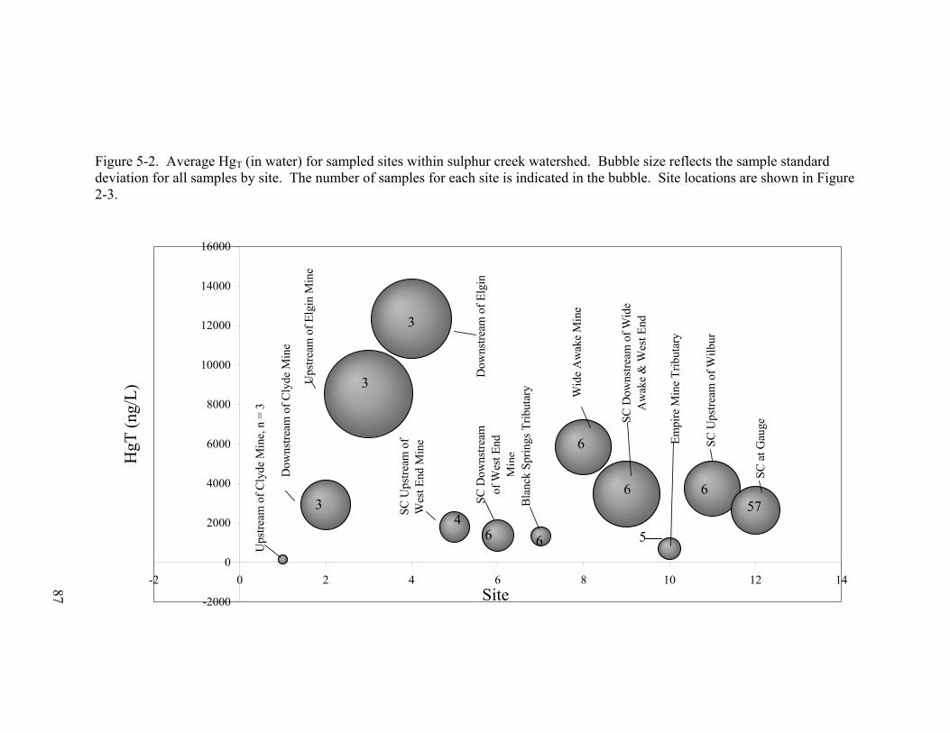
Figure 5-2. Average HgT (in water) for sampled sites within sulphur creek watershed. Bubble size reflects the sample standard deviation for all samples by site. The number of samples for each site is indicated in the bubble. Site locations are shown in Figure 2-3.

-2000

0

2000

4000

6000

8000

10000

12000

14000

16000

-2 0 2 4 6 8 10 12 14Site

HgT

(ng/

L)

Ups

tream

of C

lyde

Min

e, n

= 3

Dow

nstre

am o

f Cly

de M

ine

Ups

tream

of E

lgin

Min

e

Dow

nstre

am o

f Elg

in

i

SC U

pstre

am o

f W

est E

nd M

ine

SC D

owns

tream

of

Wes

t End

M

ine

Bla

nck

Sprin

gs T

ribut

ary Wid

e A

wak

e M

ine

ib

SC D

owns

tream

of W

ide

Aw

ake

& W

est E

nd

Empi

re M

ine

Trib

utar

y

SC U

pstre

am o

f Wilb

ur

Si

SC a

t Gau

ge

3

3

6

6 6 3 57

4 6 5 6

87

Figure 5-3. Average MeHgT (in water) for sampled sites within Sulphur Creek watershed. Bubble size reflects the sample standard deviation for all samples by site, except for hatched bubbles, as noted. The number of samples for sites with more than two samples is indicated in the bubble. Site locations are shown in Figure 2-3.

Denotes n = 2, No Standard Deviation Information for Sample

-1

0

1

2

3

4

5

-2 0 2 4 6 8 10 12 14

Site

MeH

gT (n

g/L)

Ups

tream

of C

lyde

Min

e

Dow

nstre

am o

f Cly

de M

ine

Ups

tream

of E

lgin

Min

e

Dow

nstre

am o

f Elg

in M

ine

SC

Ups

tream

of

Wes

t End

Min

e

SC

Dow

nstre

am

of W

est E

nd M

ine

Bla

nck

Spr

ings

Trib

utar

y

Wid

e A

wak

e M

ine

Trib

utar

y

Em

pire

Min

e Tr

ibut

ary SC

Ups

tream

of W

ilbur

S

i

SC

at G

auge

SC

Dow

nstre

am o

f Wid

e A

wak

e &

Wes

t End

3

2277

8

8

89

Figure 5-4. Total mercury concentrations (ng/mg, ppm) in fine-grained sediment in the upper (a) and lower (b) parts of the Sulphur Creek watershed (RWQCB-CV 2004b).

a)

b)

90

Figure 5-5 shows a plot of the all of available total mercury (ng/L) data against

instantaneous flow (cfs) for Sulphur Creek at the USGS gage (n = 56), collected over

the 1997 – 2004 time period. While most of these data were collected at long time

intervals (weeks or months apart), 19 of the data were collected during a 30 hour time

period at 1.5 to 3 hour time intervals in February of 2004. The flow/HgT relationship

is modeled as a lognormal distribution independent of flow for flows less than 55 cfs

and as a ln-ln linear model for flows greater than 55 cfs. The circled values represent

three flows at the rising limb of a hydrograph in response to a storm event. The HgT

value is thus sensitive to the time rate of change in flow, as well as to the current flow.

This complexity is discussed further in the next section on the available time series

data. Unfortunately, only mean daily flow data are available. At this time scale, the

hysteresis in the flow/HgT relationship is manifested as random scatter in the flow/HgT

model. Hysteresis in HgT concentration and loads is described and demonstrated in

the next section.

Figure 5-6 shows the relationship between instantaneous flow and HgT/TSS

(the ratio of total mercury concentration in water in ng/L to the concentration of total

suspended solids in mg/L). HgT/TSS is used as a surrogate for the concentration of

total mercury in fine-grained suspended sediment. Dry season values are assumed to

be lognormally distributed independently of flow. Wet season values are partitioned

by flows > 55 cfs and flows < 55 cfs. Within these flow ranges, the values are

assumed to lognormally distributed independent of flow (see Appendix B for normal

probability plots of HgT/TSS in log space by season and flow regime, Figures B.1,

B.2, and B.3). The first rains of the season show a “first flush” effect, with relatively

large Hg/TSS values. This is thought to result from the mobilization of geothermal

spring precipitates and colloidal HgS(s) that have deposited during the dry season. The

wet season data include longer-term data shown as white circles (1997-2004) and data

from a single storm event in February, 2004. While the relationship between flow and

HgT/TSS is very noisy, the long-term and single-storm data overlap well.

Figure 5-5. Instantaneous flow versus total mercury concentration for Sulphur Creek, all data.

y = 1.2076x1.5554

R2 = 0.5716

1

10

100

1000

10000

100000

0 1 10 100 1000

Flow (cfs)

HgT

, ng/

L

Flow < 55 cfs

LN Flow > 55 cfs

Avg HgT, All Data

Avg HgT, Flow < 55 cfs

91

1

10

100

1000

0.1 1 10 100 1000

Flow (cfs)

HgT

/TSS

, ppm

Dry Season Wet Season Single Storm Data (2/04) "First flush"

11/07/00

11/20/01

Single Storm, 2/04

Wet Season,All Data

Dry Season,All Data

55 cfs

Figure 5-6. Relationship between HgT/TSS and flow by water season (mean daily flow) and for a single storm event (instantaneous flow) (2/2004).

92

93

SULPHUR CREEK HGT, HGT/TSS LOADING TIME SERIES DATA

Figure 5-7 shows the time series for HgT, TSS, HgT/TSS, and flow for a 30-hour

period (time step of 1.5 – 3.0 hours) on February 25/26, 2004, which included a storm

event (“autosampler data”). The relationship between instantaneous flow and HgT

shown in Figure 5-7 collected for this single event is similar to the relationship

between the instantaneous flow and HgT data collected days, weeks, months apart

(Figure 5-5 includes both the autosampler data and the hand collected data). However,

several patterns emerge which emphasize the complexity of mercury/sediment

transport. For example, the residual errors in a plot of ln(flow) versus ln(HgT) in the

time series data show significant autocorrelation. The Durbin-Watson statistic for this

data set is 0.72, which is much less than the lower rejection level of 1.18 for 19 data

points and one predictor variable, supporting the rejection of the hypothesis that the

residuals are not autocorrelated (Chatterjee et al. 2000). Figure 5-8 shows a plot of the

first-order residual error at time “t” (Residualt) versus the residual error for the

preceding time step (Residualt-1). A plot of the second-order residuals (Residualt

versus Residualt-2) shows no significant correlation, suggesting that the autoregressive

structure is approximately first-order for this time series.

Since most of the mercury comprising the total mercury concentration is

associated with suspended sediment, the relationship between HgT and flow can be

understood in terms of the relationship between suspended sediment transport (or TSS

transport), the grain size distribution, and flow or stream power. For example, Figure

5-9 shows that HgT load versus discharge displays a hysteresis loop typical of

suspended sediment load. Figure 5-10 shows the relationship between the time step

change in HgT (HgT,t – HgT,t+1) with the change in flow (Flowt – Flowt+1) during the

storm event of 2/25-6/2004. In general, the “falling limb” of a storm event

hydrograph carries less sediment than the “rising limb” (Dunne and Leopold 1978).

9

4 Figure 5-7. Time series data for HgT, TSS, HgT/TSS, and flow for 2/25-6/2005. Data are from the Sulphur Creek TMDL report (RWQCB-CV 2004b).

0.1

1

10

100

1000

10000

0 5 10 15 20 25 30

Time (Hours)

Con

cent

ratio

n or

Flo

w U

nits

)

TSS (mg/L)

Hg/TSS (ppm)

Flow (cfs)HgT (ng/L)

Figure 5-8. Test for first-order autoregressive structure in the Log(flow) vs Log(HgT) autosampler data. The plot shows the residual (predicted HgT – observed HgT) for a time step “t” (“Residualt”) versus the residual for the previous time step (“Residualt-1”). Data are from the Sulphur Creek TMDL report (RWQCB-CV 2004b).

y = 0.6x + 0.0358R2 = 0.3938

-1

-0.5

0

0.5

1

1.5

2

-1 -0.5 0 0.5 1 1.5 2

Residualt

Res

idua

l t-1

95

50

100

150

200

250

300

350

400

Hg

Load

(g/h

r)

96

00 100 200 300 400

Discharge (cfs)

Sediment transport is a complicated phenomenon and is incompletely understood. In

the case of the Sulphur Creek TMDL, data on the particle size distribution and direct

measurements of stream velocity are missing. Given this state of affairs and the

magnitude of the other uncertainties in this decision problem, the simple flow versus

HgT model shown in Figure 5-5 was used to simulate HgT loading patterns. Table 5-1

compares the predicted HgT and HgT load results from this model with the calculated

HgT and HgT load values from the time series observations. The predictions match

the observed values fairly well, but the comparison is based on very few data. While

this check is inconclusive, it represents all of the available data for decision support.

Figure 5-9. Hysteresis in HgT load versus discharge, with arrows indicating time direction. Data are from the Sulphur Creek TMDL report (RWQCB-CV 2004b).

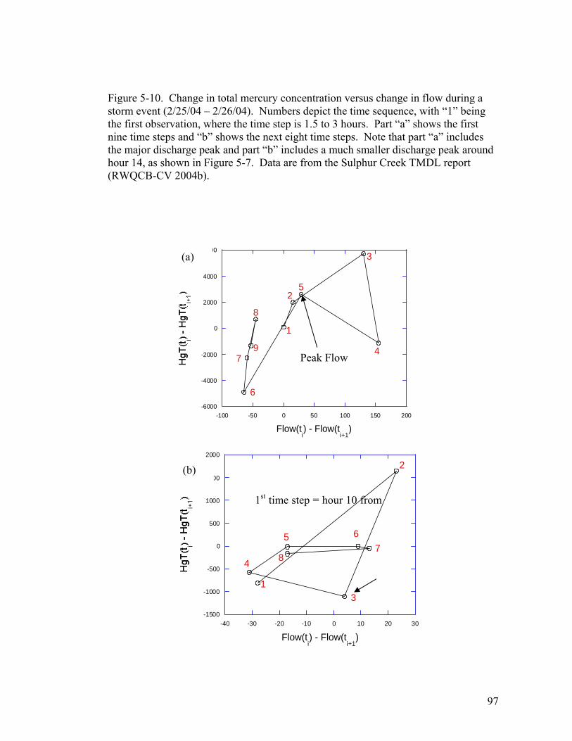
97

-6000

-4000

-2000

0

2000

4000

6000

-100 -50 0 50 100 150 200

Flow(ti) - Flow(t

i+1)

1

2

3

4

5

6

7

8

9

Figure 5-10. Change in total mercury concentration versus change in flow during a storm event (2/25/04 – 2/26/04). Numbers depict the time sequence, with “1” being the first observation, where the time step is 1.5 to 3 hours. Part “a” shows the first nine time steps and “b” shows the next eight time steps. Note that part “a” includes the major discharge peak and part “b” includes a much smaller discharge peak around hour 14, as shown in Figure 5-7. Data are from the Sulphur Creek TMDL report (RWQCB-CV 2004b).

(a)

Peak Flow

-1500

-1000

-500

0

500

1000

1500

2000

-40 -30 -20 -10 0 10 20 30

Flow(ti) - Flow(t

i+1)

1

2

3

4

5 67

8

(b)

1st time step = hour 10 from

98

Table 5-1. Mean daily HgT and daily HgT loading prediction for 2/25/04 using mean daily flow versus estimation of mean daily HgT and daily HgT loading from observed time series values. Data are from the Sulphur Creek TMDL report (RWQCB-CV 2004b).

Predicted HgT1, ng/L

(95% confidence interval)

Estimated HgT

2, ng/L

Predicted HgT Loading1, g/day (95% confidence interval)

Estimated HgT Loading2, g/day

2600 (680 – 9,900) 3000 920 (240 – 3,500) 1600

Notes: 1) Mean daily values predicted from mean daily flow using model. 2) Mean daily values estimated from summation over time step observations.

METHYLMERCURY DATA

Most of the limited methylmercury data within the Sulphur Creek watershed

were collected at the USGS gage (Figures 5-3, 2-3). Looking more closely at these

data, several things are apparent. First, the data set (including both wet and dry season

samples) appears to be approximately lognormally distributed (Figure 5-11).

Secondly, the MeHgT data show a distinct seasonality, with distinct very high values

in the hot, low flow months of July and August. Figure 5-12 shows the seasonal trend

of the MeHgT sample average. One possible explanation for this seasonality is that the

microbial activity of mercury methylating bacteria is very high in July and August due

to in part to low flow conditions and high temperatures (low dissolved oxygen).

99

Figure 5-11. a) Histogram of MeHgT data from the Sulphur Creek gage in log space (RWQCB-CV 2004b). Data frequencies are represented by bars (NOTE: bins are not evenly spaced). Model frequencies for a lognormal distribution using the sample average and standard deviation are shown by the dashed line. Twice as many data were collected in the wet season (n = 18) relative to the dry season (n = 9). b) The histogram over the data in arithmetic space is shown for comparison.

igure 5-11. a) Histogram of MeHg

T data from the Sulphur Creek gage in log space (RWQCB-CV 2004b). Data frequencies are represented by bars (NOTE: bins are not evenly spaced). Model frequencies for a lognormal distribution using the sample average and standard deviation are shown by the dashed line. Twice as many data were collected in the wet season (n = 18) relative to the dry season (n = 9). b) The histogram over the data in arithmetic space is shown for comparison.

0

0.05

0.1

0.15

0.2

0.25

0.3

0.35

-1.21

Frqu

ency

0

0.05

0.1

0.15

0.2

0.25

0.3

0.35

e

-0.71 -0.20 0.30 0.81 More

Bin Log(MeHgT)

Data Lognormal model simulation

0

0.1

0.2

0.3

0.4

0.5

0.6

0.7

0 1 2 3 4 5 6 7 8 9 10 11 12 13 14 15 16 17 18More

MeHgT (ng/L)

Freq

uenc

y

b)

a)

1

00 Figure 5-12. Seasonal Trend in Average MeHgT. The dry season data includes the three data broken out in the July/August

average. Data are from the Sulphur Creek TMDL report (RWQCB-CV 2004b).

-5

0

5

10

15

20

25

30

Wet Dry July/August

Water Season/Month

Ave

rage

MeH

gT (n

g/L)

n = 18

n = 9

n = 3

101

While there is no discernible pattern between HgT and MeHgT in Sulphur

Creek, some trends do appear at the larger scale of the Cache Creek watershed. Figure

5-13 plots the average of log(HgT) against the average of log(MeHgT) for each site

with data in the Cache Creek watershed. The Sulphur Creek and Upper & Mid-Bear

Creek data are grouped because of significant local geothermal influences not present

at the other sites. While these groupings indicate that HgT and MeHgT correlate at the

scale of the Cache Creek watershed, missing data on other important predictive

variables at this scale (sulfate concentration, dissolved organic carbon concentration,

reactive mercury concentration in sediment concentration) prevent a causal

interpretation of this relationship. The causal probabilistic model used to predict

MeHgT is discussed in Chapter 6.

R2 = 0.6323

-1.4

-1.2

-1.0

-0.8

-0.6

-0.4

-0.2

0.00 0.5 1 1.5 2 2.5 3 3.5

Average(Log(HgT))

Ave

rage

(Log

(MeH

gT))

Sulphur and Upper/Mid Bear Creeks Other Cache Creek Sites

NorthFork

SouthFork

Davis Creek

Yolo

Rumsey

Harley Gulch

SulphurCreek

Upper BearCreek

Lower Bear Creek

Mid BearCreek

1

02 Figure 5-13. A plot of the average of the log-transformed HgT data (Average Log(HgT)) versus the average of the log-transformed

MeHgT data (Average log(MeHgT)) for sites within cache creek watershed. Data are grouped for Sulphur Creek and Upper, Mid- Bear Creeks because of significant geothermal spring and ground water sources not present at the other sites. These sources provide significant loads of total mercury and methylmercury, sulfate, nutrients, and DOC (Rytuba 2005b).

103

5.2 A CONCEPTUAL MODEL OF THE SULPHUR CREEK MERCURY TMDL

AS AN INFLUENCE DIAGRAM

Figure 5-14 shows a high level conceptual model of the behavior of mercury in the

Sulphur Creek watershed, as observed at the gage, represented as an influence

diagram. At the highest level, this model shows the relationship of potential controls

(“Potential Control Decision”), the variables that could be influenced by control

projects (“Annual HgT Loading” and “HgT/TSS”), and the variables that are valued by

decision-makers in this decision (“Annual HgT Loading” and “Annual MeHgT

Loading”), as indicated by the arcs from these variables to the “Strategy Value” node.

This model includes the uncertain environmental relationships between total mercury

loading (“Annual HgT Loading”), total mercury concentration in total suspended

solids (TSS) (“HgT/TSS”), methylmercury concentration in water (“[MeHgT]w”), and

methylmercury loading (“Annual MeHgT loading”), conditioned on water year

(“Wet/Dry Year”) and/or season, as indicated by the presence of an arc (“Water

Season”: wet or dry). The environmental variables shown in Figure 5-14 reflect sets of

probability distributions over loadings and concentrations observed at the gage for a

particular water season in a wet or dry year. The posterior distribution over an

environmental variable takes into consideration wet and dry years and the wet and dry

season within a water year, so that its distribution reflects the full range of hydrologic

conditions. These variables could be defined at other spatial and temporal scales, but

the scale shown reflects the level of aggregation appropriate for this TMDL decision.

It is important to note that the appropriate time and spatial scales for variable

definitions should be determined by the decision-makers’ goals and objectives, not by

technical considerations. The basis for this statement is the use of the Bayesian

definition of probability. Of course, decision participants may choose to use scales

supported by technical considerations, but this point is noted to emphasize the

importance of the decision situation in the definition of variables.

104

Details about the construction of these probability distributions are described

in detail in Chapter 6. The models and methods used include consideration of the

partially-understood physical, chemical, and biological processes that drive the

movement and fate of mercury species in the Sulphur Creek watershed and the

available data. With too little causal detail, the probability distributions are very

difficult to interpret and to construct. Sub-models are used to represent the additional

detail needed to perform the later construction of the needed probability tables. Figure

5-15 shows the more detailed causal influence diagram used to construct these tables.

105

Figure 5-14. Conceptual model relating the highly uncertain relationship between annual total mercury (HgT) loading and annual total methylmercury (MeHgT) loading at the Sulphur Creek gage as a causal influence diagram.

1

06 Figure 5-15. More detailed Sulphur Creek mercury TMDL conceptual model, expanding the sub-models shown in the influence

diagram shown in Figure 5-14.

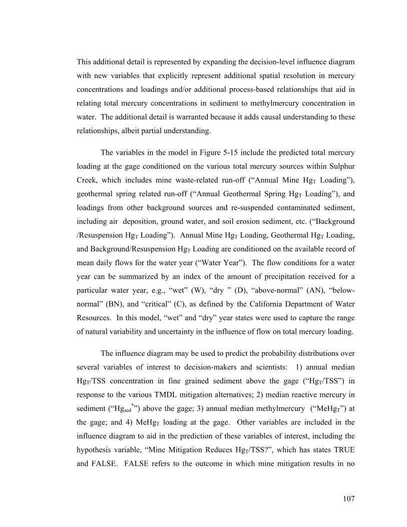
107

This additional detail is represented by expanding the decision-level influence diagram

with new variables that explicitly represent additional spatial resolution in mercury

concentrations and loadings and/or additional process-based relationships that aid in

relating total mercury concentrations in sediment to methylmercury concentration in

water. The additional detail is warranted because it adds causal understanding to these

relationships, albeit partial understanding.

The variables in the model in Figure 5-15 include the predicted total mercury

loading at the gage conditioned on the various total mercury sources within Sulphur

Creek, which includes mine waste-related run-off (“Annual Mine HgT Loading”),

geothermal spring related run-off (“Annual Geothermal Spring HgT Loading”), and

loadings from other background sources and re-suspended contaminated sediment,

including air deposition, ground water, and soil erosion sediment, etc. (“Background

/Resuspension HgT Loading”). Annual Mine HgT Loading, Geothermal HgT Loading,

and Background/Resuspension HgT Loading are conditioned on the available record of

mean daily flows for the water year (“Water Year”). The flow conditions for a water

year can be summarized by an index of the amount of precipitation received for a

particular water year, e.g., “wet” (W), “dry ” (D), “above-normal” (AN), “below-

normal” (BN), and “critical” (C), as defined by the California Department of Water

Resources. In this model, “wet” and “dry” year states were used to capture the range

of natural variability and uncertainty in the influence of flow on total mercury loading.

The influence diagram may be used to predict the probability distributions over

several variables of interest to decision-makers and scientists: 1) annual median

HgT/TSS concentration in fine grained sediment above the gage (“HgT/TSS”) in

response to the various TMDL mitigation alternatives; 2) median reactive mercury in

sediment (“Hgsed*”) above the gage; 3) annual median methylmercury (“MeHgT”) at

the gage; and 4) MeHgT loading at the gage. Other variables are included in the

influence diagram to aid in the prediction of these variables of interest, including the

hypothesis variable, “Mine Mitigation Reduces HgT/TSS?”, which has states TRUE

and FALSE. FALSE refers to the outcome in which mine mitigation results in no

108

discernable change in annual median HgT/TSS because of the high background

mercury sources. TRUE refers to the outcome in which mine mitigation reduces

HgT/TSS during wet season flows to the regional background level of 1 - 10 ppm.

“Percent Reactive HgT” refers to the fraction of HgT/TSS that contributes to the pool

of reactive mercury in sediment.

The structure of the model reflects the fact that mercury methylation is

believed to be controlled by the concentration of reactive mercury in sediment

(Hgsed*) and the “level of microbial activity” of bacterial species that methylate

reactive mercury in-situ. There is no direct information on the concentrations of

reactive mercury in sediment in Sulphur Creek. However, some relevant information

is available from mercury methylation potential studies in the Cache Creek watershed

(Bloom 2001; Domagalski et al. 2003; Suchanek et al. 2004) and studies from other

watersheds (Benoit et al. 2003; Marvin-DiPasquale 2005). In this model, Hgsed* is

conditioned by Annual Average Hg/TSS at Gage and Percent Reactive Hg in

HgT/TSS. While the uncertainty in Hgsed* is very large, this structure suggests that

observed Hg/TSS provides relevant information about concentration and that the

source of the mercury (mines/geothermal/soils) provides some limited information

about speciation.

The use of hypothesis variables to describe the effectiveness of mine

mitigation in reducing annual average HgT/TSS (Mine Reduction Reduces HgT/TSS?,

“HgT/TSS reduction hypothesis”) and the percentage of reactive mercury in sediment

(Percent Reactive Hg in Sediment?, “percent reactive mercury hypothesis”) is a

reflection of the fact that both variables will remain unobserved before the decision is

made. While research could do much to inform the HgT/TSS reduction hypothesis,

that variable can not be completely resolved until mine mitigation has been performed

and the remaining contaminated sediment has been partially flushed from the creek.

The percent reactive mercury hypothesis variable could be observed before the

decision is made, but this was determined to be too expensive by decision-makers.

The use of hypothesis variables allows decision-makers to consider the decision to

109

collect more information about these hypotheses in terms of TMDL decision value, the

current state of information, and a consideration of which other variables could also be

observed in the future. This allows much more robust information collection decisions

to be made, formalizing many of the intuitive approaches currently used (Howard

1970).

The state of the “microbial activity” variable can also be thought of as a

hypothesis variable, since it cannot be directly observed. Instead, it should be thought

of as a useful construct that describes the aggregate effect of the many factors that we

partially understand as influencing the efficiency of the microbial methylation of

mercury (Marvin-DiPasquale 2005). For example, it could be modeled as being

conditionally dependent on seasonal sulfate and sulfide concentrations, temperature,

flow conditions (redox conditions), etc. Also, the state of microbial activity can be

updated based on a test set of current or future observations of methylmercury data. It

is in this sense that “microbial activity” can be thought of as a hypothesis variable in a

Bayesian network.

This model represents the current understanding of the available experts and

decision-makers of the relationships between potential mercury TMDL mitigation

strategies and the environmental targets of interest, total mercury and methylmercury

loads exported from the Sulphur Creek watershed. Contrary to typical water quality

model development practice, the purpose of this model is not to replace less realistic

models, but rather to provide an alternative model framework specifically for decision

support. In addition to probabilistic causal representation of a complex environmental

system, modeling for decision support should provide decision-makers with an

understanding of the meaning of predictive uncertainty in the context of the decisions

being made and in terms meaningful to decision-makers. This obviously goes beyond

the purposes and methods of traditional water quality modeling and potentially enters

into the many sub-fields that make use of results from the decision sciences, including

“decision support”, decision analysis, multi-criteria decision-making, the analytic

hierarchy process, and others.

110

This chapter concludes with a precise definition of the states for each of the

variables shown in Figure 5-15. Table 5-2 lists each variable and its type (chance,

hypothesis, deterministic, or decision) and defines the states for each. The generation

of the probability distributions over the states of the variables shown in Table 5-2 and

the decision analytical use of the fully-specified influence diagram model will be

shown in subsequent chapters.

Variable Name Variable Type States Definition

Model/ Expertise/ Data

Source

TMDL Strategy Decision Decision

Mine Mitigation, Geothermal & Mine Mitigation, and Status Quo

Mine mitigation is the alternative in which HgT loadings from mines are reduced according to the load allocation scheme explained in Chapter 2. Geothermal & mine mitigation includes the mine reductions from the Mine Mitigation alternative, but also includes HgT load reductions from geothermal springs. The Status Quo alternative refers to the conclusion from a use attainability analysis that the current beneficial uses are inappropriate given background loadings and includes a public information campaign. See Chapter 2 for more details.

Not applicable

Water Year Chance Wet, Dry

CA Dept of Water Resources (DWR) Index for the Sacramento River . A wet year (W) is defined by a combined discharge ≥ 9 maf. A dry year (D) is defined by a combined discharge > 5.4 maf but ≤ 6.5 maf. See the footnote to Figure 5-1 for more information.

Definition from CA DWR

Water Season Chance Wet, Dry Dry = March 31 to September 30; Wet = Rest of year Definition from RWQCB-CV (2005b)

Annual Mine HgT Loading Chance Low, High Low = 1 kg/year, High = 20 kg/year

Expert judgment informed by limited data

Background/Resuspension HgT Loading Chance Low, High Low = 1 kg/year,

High = 20 kg/year


Annual Geothermal Spring HgT Loading Chance Low, High Low = 0.1 kg/year,

High = 4 kg/year


Annual HgT Loading at Gage Deterministic LLL, LLH, LHL,

LHH, etc. Functionally determined sum of parents Simulation

111

Table 5-2. Definitions of variables used in the influence diagram shown in Figure 5-15.

Variable Name Variable Type States Definition Model/ Expertise/ Data Source

Annual Average HgT/TSS at Gage Chance Low, Nominal, High Low = 1 ppm, Nominal = 10 ppm,

High = 100 ppm Expert judgment informed by limited data

Mine Mitigation Reduces HgT/TSS? Hypothesis True, False True = HgT/TSS reduced to regional

background levels, False = No change Expert judgment informed by other studies

Reactive Mercury in Sediment Chance Low, High Low = 0.0001 ppm, High = 5 ppm Expert judgment informed by limited data

Percent Reactive Mercury HgT/TSS? Hypothesis Low, High Low = 0.01%, High = 5% Expert judgment informed by

other studies

Microbial Activity Hypothesis Low, HighHigh = 5 times more efficient methylation for a given Hgxed

* concentration relative to Low.

Expert judgment informed by other studies

Annual Median [MeHgT]w Chance Low, Nominal, High Low = 0.05 ng/L, Nominal = 1 ng/L, High = 5 ng/L Simulation

Annual MeHgT Loading at Gage Chance Low, Nominal, High Low = 0.25 g/year, Nominal = 5 g/year,

High = 100 g/year Simulation

Table 5-2. (Continued)

1

12

113

5.3 REFERENCES

Benoit, J. M., Gilmour, C., Mason, R., and Heyes, A. (1999). "Sulfide Controls on Mercury Speciation and Bioavailability to Methylating Bacteria in Sediment Pore Waters." Environmental Science & Technology, 33(6), 951- 957.

Benoit, J. M., Gilmour, C. C., Heyes, A., Mason, R. P., Miller, C. L., and Aiken, G. R. (2003). "Geochemical and Biological Controls over Methylmercury Production and Degradation in Aquatic Systems

Constants for Mercury Binding by Dissolved Organic Matter Isolates from the Florida Everglades." Biogeochemistry of Environmentally Important Trace Metals, 65(24), 4445-4451.

Bloom, N. (2001). "Solid Phase Mercury Speciation and Incubation Studies in or Related to Mine-site Run-off in the Cache Creek Watershed (CA)." CALFED.

Chatterjee, S., Hadi, A. S., and Price, B. (2000). Regression analysis by example, Wiley, New York.


Domagalski, L., J., Alpers, N., C., Slotton, G., D., Suchanek, H., T., and Ayers, S. M. (2004). "Mercury and Methylmercury Concentrations and Loads in the Cache Creek Basin, California, January 2000 through May 2001." U.S. Geological Survey.

Domagalski, J. L., Slotton, D. G., Alpers, C. N., Suchanek, T. H., Churchill, R., Bloom, N., Ayers, S. M., and Clinkenbeard, J. (2003). "Summary and Synthesis of Mercury Studies in the Cache Creek Watershed, California, 2000-01." CALFED.

Dunne, T., and Leopold, L. B. (1978). Water in Environmental Planning, W.H. Freeman and Company, New York.

Goff, F., Bergfeld, D., and al, e. (2001). "Geochemical Data on Waters, Gases, Rocks, and Sediments from the Geyser-Clear Lake Region, California (1991-2000)." Los Alamos National Laboratory.

Howard, R. A. (1970). "Decision Analysis: Perspectives on Inference, Decision and Experimentation." IEEE Special Issue, Detection Theory and Applications, 632-643.

Kim, C. S., Rytuba, J. J., and Brown, G. E., Jr. (2004). "Geological and Anthropogenic Factors Influencing Mercury Speciation in Mine Wastes: An EXAFS Spectroscopy Study." Applied Geochemistry, 19(3), 379-393.

Lowry, G. V., Shaw, S., Kim, C. S., Rytuba, J. J., and Brown, G. E., Jr. (2004). "Macroscopic and Microscopic Observations of Particle-Facilitated Mercury Transport from New Idria and Sulphur Bank Mercury Mine Tailings." Environmental Science & Technology, 38(19), 5101-5111.

114

Marvin-DiPasquale, M. (2005). "Mercury methylation potential and percent reactive mercury ranges for various environments." Menlo Park, CA, Personal Communication to William Labiosa.



Rytuba, J. J. (2003). "Mercury From Mineral Deposits and Potential Environmental Impact." Environmental Geology, 43, 326-338.

Rytuba, J. J. (2005a). "Background total mercury and methylmercury loadings in Sulphur and Bear Creeks, unpublished data." Personal Communication to William Labiosa.

Rytuba, J. J. (2005b). "Mercury Speciation in Sulphur Creek." Menlo Park, CA, Personal Communication to William Labiosa.

Slotton, D. G., Ayers, S. M., Suchanek, T. H., Weyand, R. D., and Liston, A. M. (2004). "Mercury Bioaccumulation and Trophic Transfer in the Cache Creek Watershed of California, in Relation to Diverse Aqueous Mercury Exposure Conditions." CALFED.

Slowey, A. (2005). "Speciation of reactive mercury in sediment." Stanford, CA. Suchanek, T., Slotton, D., Nelson, D., Ayers, S., Asher, C., Weyand, R., Liston, A.,

and Eagles-Smith, C. (2004). "Mercury Loading and Source Bioavailability from the Upper Cache Creek Mining Districts." CALFED, 72.

115

CHAPTER 6: SULPHUR CREEK MERCURY TMDL SOURCE AND

LINKAGE ANALYSIS USING A BAYESIAN NETWORK APPROACH

This chapter briefly reviews current practice in TMDL source analysis and

linkage analysis, as relevant to the mercury TMDL case study used in this work. It

also presents a probabilistic mercury source analysis and linkage analysis for the

Sulphur Creek mercury TMDL that organizes the results as probability tables. These

probabilistic data are then integrated into a Bayesian network model (influence

diagram) that serves as the basis for TMDL decision analysis and decision support, the

subject of Chapter 8.

6.1 CURRENT PRACTICE IN MERCURY-MINE IMPACTED WATERSHED

SOURCE AND LINKAGE ANALYSIS

DETERMINISTIC TOTAL MERCURY SOURCE ANALYSIS

The TMDL reports for the Sulphur Creek and Cache Creek, Bear Creek, and Harley

Gulch mercury TMDLs present typical deterministic approaches for estimating annual

budgets for water, total mercury, methylmercury, and sediment. The available data for

these TMDLs consist of mean daily flows measured at the gage stations shown in

Figures 2-2 and 2-3 for 1995 – present (some missing data) and the available relevant

water quality data for selected dates: instantaneous total mercury, methylmercury, and

total suspended solids concentrations (HgT, MeHgT, and TSS, respectively). TSS is

used as a surrogate for suspended sediment concentration and HgT /TSS is used as a

surrogate for total mercury concentration in fine-grained sediment (RWQCB-CV

2004b). Table 6-1 summarizes the available relevant water quality data for Sulphur

Creek and Lower Bear Creek, the stream segments focused on in this paper. As an

illustration of the amount of available data, the number of HgT data for all stream

segments within the Cache Creek watershed range from 16 to 65, with a mean of 30.

The annual water budget was estimated by summing mean daily flows over a

given water year for gaged stream segments. Water budgets for ungaged segments

were estimated from a version of the rational runoff method or, in some cases, using

the assumption that the percentage discharge from a sub-basin could be directly

approximated by its areal percentage of the watershed (Dunne and Leopold 1978).

The Regional Water Quality Control Board (RWQCB) staff’s approach for estimating

annual loads (LAnn) involves multiplying the mean daily flow (mdf) by the water

quality concentration predicted for that flow (C(mdf)) to calculate the mean daily load,

then summing over the water year:

It should be kept in mind that estimates of total mercury loadings within

Sulphur Creek and the other stream segments in Cache Creek have significant

associated uncertainties. While estimating the annual water budget from gaged flows

For some stream segments (South Fork, Cache Creek at Rumsey, and Cache Creek at

Yolo), stream flow appears to be linearly correlated with HgT and TSS over the entire

observed flow range. For these segments, C(mdf) was deterministically estimated

from linear correlations of the untransformed variables. For the other stream

segments, the arithmetic averages of HgT and TSS were used to estimate C(mdf). For

MeHgT, arithmetic averages were used for all segments to estimate C(mdf). The use

of arithmetic averages and linear models with no transformation of the variables for

predicted concentrations implies that the variables/residuals are normally distributed,

an assumption that is not supported by the data in several cases. As shown in Chapter

5, hysteresis in the C(flow) relationship at the scale of individual storm events may

account for much of the scatter in the log-log linear regions of the HgT (TSS) versus

flow relationship.

∑=wateryear

Ann mdfCmdfL )(*

116

117

is operationally straightforward25, predicted total mercury concentrations are used in

the annual HgT load estimates. Since the associated prediction errors are quite large

relative to the predicted means and the concentrations appear to be lognormally

distributed in most cases, a probabilistic estimate of average annual loadings based on

log transformed concentration values is more informative than the typical

deterministic estimation approaches. It should be noted that additive errors in a

lognormal flow vs. concentration model reflect the fact that the

Table 6-1. Sulphur Creek and Lower Bear Creek Data Summary, from Cache Creek Mercury TMDL Report (RWQCB-CV 2004a) and Sulphur Creek TMDL Report (RWQCB-CV 2004b).

Stream Segment

Water Quality Parameter

Number of observations Range Mean /

Median HgT (ng/L) 34 245 – 16,410 2,890 /

1,094 MeHgT (ng/L) 27 0.1 – 21 2 / 1 TSS (mg/L) 31 4 – 1,372 214 / 56

HgT (ng/L), 2/25/04 Storm Event 19 231 – 9,510

2,540 / 1,440

Sulphur Creek

TSS (ng/L), 2/25/04 Storm Event 19 1.8 – 1,390 416 / 173

HgT (ng/L) 16 18.5 – 1,290 281 / 81.9 MeHgT (ng/L) 1 0.82 NA

Lower Bear

Creek TSS (mg/L) 15 1.7 - 670 118 / 29.3

scatter in the underlying untransformed data is proportional to flow. By log-

transforming the flow and concentration variables, the residuals in log-space obey the

assumptions behind the linear regression model for the selected flow ranges.

DETERMINISTIC MERCURY LINKAGE ANALYSIS

While inorganic mercury associated with particulates is often the dominant mercury

fraction in aquatic environments, methylmercury is the chemical species that

25 While the estimation method is straightforward, the estimate has significant uncertainty.

118

bioaccumulates and biomagnifies in aquatic food webs, potentially resulting in fish

tissue mercury levels that are toxic to humans and wildlife (Benoit et al. 2003).

Although most fish advisories apply to watersheds dominated by atmospherically

deposited mercury (Wiener et al. 2003), this research focuses on a watershed impacted

by relatively large total mercury inputs from legacy mine wastes, active geothermal

sources, and high regional background levels in soils. In the creeks in this watershed,

like most aquatic environments, in situ microbially mediated methylmercury

production from available reactive inorganic mercury at the oxic/anoxic sediment

interface is believed to be the dominant source of methylmercury. While

methylmercury formation is positively correlated with total mercury concentration in

the Cache Creek watershed and many other watersheds, environmental factors other

than total mercury loading (e.g., sulfate and sulfide sediment concentrations, dissolved

organic carbon (DOC) levels, temperature, etc.) may strongly influence

methylmercury concentrations and bioaccumulation in aquatic ecosystems (Benoit et

al. 2003; Wiener et al. 2003). In general, the range of mercury methylation rates

across aquatic ecosystems is greater than the range in total mercury loading rates

(Benoit et al. 2003). In fact, it may be the case that high methylmercury

concentrations may be more of a localized “hotspot problem” under conditions of high

microbial activity and high reactive mercury than a watershed-wide mercury

contamination problem (Calfed Bay-Delta Program 2005). However, this issue is still

an active area of research (Marvin-DiPasquale 2005).

The observed aqueous MeHg concentration at any point in time integrates the

many processes influencing MeHg production and loss (Benoit et al. 2003). Relevant

factors include total mercury loadings, reactive mercury concentrations in sediment,

low flow duration, and temperature, all of which vary spatially and temporally. Even

with ample data on the most relevant environmental factors, there is significant

uncertainty in predicting the value of MeHgT for a given set of conditions. In practice,

the data on the most relevant environmental factors (reactive mercury concentration in

sediment, acetate and lactate concentrations, sulfate and dissolved sulfide

119

concentrations in sediment, pore water temperature, etc.) are very sparse or missing

altogether for the watershed of interest.

The large uncertainties in linking total mercury concentrations and loadings to

methylmercury concentrations and loadings are widely acknowledged. At present,

trustworthy process-based models of the formation of methylmercury do not exist and

the available empirical (statistical) models based on aqueous concentrations of total

mercury (HgT) and total methylmercury (MeHgT) lack clear causal predictive power.

While semi-empirical methylmercury predictive models based on the concentration of

reactive mercury in sediment (Hgsed, rct) and microbial activity are the state of the art

(Mark Marvin-DiPasquale, personal communication), there are no data available to

describe Hgsed, rct and very little relevant data for describing microbial activity in

Sulphur Creek, other than what can be inferred from the small number of available

MeHgT, sulfate, and DOC data.

Rather than relying on a potentially non-causal empirical relationship between

HgT and MeHgT in the linkage analysis, I propose an alternative way of thinking about

the causal relationship between inorganic mercury and methylmercury, one that

focuses on the what experts know about the causal relationships between potential

controls and the environmental targets of interest, making the best use of the available

data and expertise.

6.2 CURRENT PRACTICE IN DEALING WITH SOURCE AND LINKAGE

ANALYSIS UNCERTAINTY

The consideration of uncertainty in TMDLs is constrained by the regulatory

requirements for the use of a Margin of Safety (MOS) and thus most discussions of

uncertainty in TMDL decisions take the MOS as a starting point. From this

perspective, an uncertainty analysis of the relevant (deterministic) models can be

performed (in theory) and, from this uncertainty analysis, the choice of an appropriate

MOS in the TMDL target can be made. The use of conservative modeling

120

assumptions, or even conservative mitigation goals, as “the MOS” is another strategy

in use. From a decision analytical point of view, the choice of “how conservative” the

MOS should be is itself a decision of fundamental importance. To leave this choice as

a conventional “scientific/engineering judgment” is to risk making a poor decision.

While a poor outcome may result from any decision under uncertainty, a good

decision means that, given the available information, the alternatives considered, and

the decision-makers’ preferences over the outcomes, the course of action chosen is the

rational one (see Chapter 4 for a discussion of utility maximization in decision

analysis).

6.3 SOURCE ANALYSIS UNCERTAINTIES AS RANDOM VARIABLES IN A

PROBABILISTIC (BAYESIAN) NETWORK

ESTIMATING PROBABILITY DISTRIBUTIONS OVER MERCURY LOADINGS

Depending on the types and amounts of available data, two basic approaches were

used to estimate the probability distributions over total mercury and methylmercury

loadings in the Sulphur Creek watershed. For the gage sites, the empirical log-log

linear model shown in Figure 5-5 was used to predict HgT from flow using Monte

Carlo simulation26. A random error term based on the residual error from Figure 5-5

was used in the simulation. Since MeHgT appears to be independent of flow

(RWQCB-CV 2004b) and approximately lognormally distributed (Figure 6-1),

simulated values from a lognormal model were used with flow data to estimate annual

MeHgT loads. To estimate the highly uncertain total mercury loadings from the

various mine sites, geothermal springs, erosion of undisturbed soil, and erosion of the

contaminated streambed, experts were asked to look at the available data for this

watershed and any other relevant data from elsewhere in the Cache Creek watershed

(Rytuba 2005a). Probability distributions for the various sources reflecting their

expert judgment were assessed and used to represent the current background state of

26 Convergence of the mean was used to limit the number of trials. Typically, 1000 to 5000 trials were

sufficient. The

121

),ln())(ln())(ln( ErrormdffmdfC

Mean daily loadings over the water year were predicted using mean daily flow data

and the total (HgT) and methylmercury (MeHgT) concentrations predicted for that

flow. The summation over the water year for the mean daily loadings is the best

estimate of the annual loading. Note that I assumed that HgT and MeHgT are

lognormally distributed (i.e., log(HgT) and log(MeHgT) are normally distributed).

Figure 6-1 shows that an assumption of lognormality leads to much better HgT and

MeHgT predictions from flow than the assumption of normality, based on the fit of

observed versus expected values. This means that using arithmetic averages and linear

models using untransformed concentration data will lead to biased predictions.

where the terms are defined as before. Note that the fact that error is assumed to be

additive in ln-space means that error is multiplicative in arithmetic space. In other

words, larger flows have larger errors for HgT, which is supported by the data. Since

the purpose of this simulation to estimate the uncertainty in the loading in any wet or

To simulate the uncertain concentration distribution over the flow-independent

range (e.g., MeHgT for all flows and HgT for flows < 55 cfs) for a given water year,

concentrations were simply randomly generated from a lognormal distribution. To

simulate uncertainty in the HgT predictions for flow greater than 55 cfs, I used a log-

log linear model that included an estimate of the prediction error based on cross-

validation using five data sub-sets (Hastie et al. 2001):

PROBABILITY DISTRIBUTION OVER THE ANNUAL TOTAL MERCURY (HGT) AND

METHYLMERCURY (MEHGT) AT THE SULPHUR CREEK GAGE

information. Discrete approximations for the loading distributions were created from

the simulated distributions using standard methods (Miller and Rice 1983; Poland

1996; Smith 1993).

+=

1

22

Figure 6-1. Observed Versus Expected Values For Normal And Lognormal Distributions For Total Mercury (HgT) and Methylmercury Concentrations (MeHgT) for All Available Data, Representing Dry and Wet Seasons and All Flow Ranges.

-1.5

-1

-0.5

0

0.5

1

1.5

-2 -1 0 1 2

Expected Value for Lognormally Distributed Value

Obs

erve

d V

alu

log(MeHgT)

-10

-5

0

5

10

15

20

25

-10 -5 0 5 10 15

Expected Value for Normally Distributed Variable

Obs

erve

d V

alu

MeHgT

2

2.5

3

3.5

4

4.5

3 3.5 4 4.5

Expected Value for Lognormally Distributed Value

Obs

erve

d V

alu

log(HgT)

-7500

0

7500

15000

22500

-10000 -5000 0 5000 10000 15000

Expected Value for Normally Distributed Variable

Obs

erve

d V

alu

HgT

123

dry water year and not to construct a time series prediction for a given set of flows in a

particular water year, the autocorrelation in the error term is not a concern (Chatterjee

et al. 2000). The scatter introduced by the hysteresis in the flow versus HgT

relationship (one of the sources of autocorrelation) is treated as random error in this

model.

A histogram over a water year’s or water season’s simulated mean daily

loadings approximates the desired loading probability distribution for that water year

or water season. The resulting probability distributions represent what we know from

the available flow and water quality data and what we do not know about the

complicated relationship between flow and HgT or MeHgT. The total uncertainty

considered includes our uncertainty in the data measurements themselves and in the

noisy relationships between flow and HgT and MeHgT. Future flow variability is

represented by a marginal distribution over water year with two states, “Wet Year”

and “Dry Year”. Based on the historical record (1906 – 2004) for the Sacramento

Valley, wet years and dry years were represented as equally probable.

Figure 6-2 shows the simulated cumulative distribution over the annual HgT

loading for Sulphur Creek in the 2000 water year, which includes flow variability,

measurement uncertainty, and HgT prediction uncertainty. Figure 6-2 also shows the

annual load estimate made using the deterministic methodology of the Central Valley

Regional Water Quality Control Board staff, which uses the arithmetic average of the

available HgT data to predict the concentration for any flow. This estimate results in a

value that occurs well beyond the 99th percentile, indicating strong high bias. This

bias results from the use of the arithmetic average of the HgT data as the measure of

central tendency, in part because wet season sampling was done more often than dry

season sampling, and, as shown in Figure 5-5, there is a significant log-log linear

correlation between flow and HgT for flows larger than 55 cfs. Also, the use of an

arithmetic average to predict HgT significantly overestimates the value for flows less

than 55 cfs, as can be seen from Figure 5-5. This results in significant load

overestimates for most of the water year.

1

24

Figure 6-2. Simulated Cumulative Distribution of Annual Total Mercury (HgT) Loading for Sulphur Creek, 2000 Water Year.

2 3 4 5 6 7 8 9

Using Arithemetic Average HgT

Deterministic HgT Load

HgT Loading (kg/year)

Average HgT Load

from Simulation

0%

100%

90%

80%

70%

60%

50%

40%

30%

20%

10% C

umul

ativ

e %

Fre

quen

cy

125

Figure 6-3 shows the correlation between the log of the best estimate annual

HgT loading and annual discharge at the Sulphur Creek gage for the period of record,

2000 – 2004. This information is summarized in Table 6-2, which also shows the

numerical values for the averages and standard deviations for the annual HgT loads for

the years of record. A “dry year” was defined using the data from the 2001 water

year, which had an average annual HgT load of 2.4 kg/year. Using the definition of

Figure 6-3. Relationship between Log(annual HgT Loading) and annual discharge at the Sulphur Creek gage.

R2 = 0.9789

0

0.2

0.4

0.6

0.8

1

0.4 0.5 0.6 0.7 0.8 0.9 1 1.1 1.2 1.3

annual discharge [106 acre-ft/yr]

log(

annu

al H

gTLd

) [kg

/yr]

126

Table 6-2. Statistical summary from simulation of annual total mercury load at the Sulphur Creek gage.

Water Year Annual Discharge (106 Acre-ft/yr)

Average Annual HgT Load (kg/yr)

Standard Deviation for HgT Load (kg/yr)

2000 0.83 3.6 0.7

2001 0.53 2.4 0.8

2002 1.0 6.2 3.8

2003 1.2 8.0 3.1

wet year as an annual discharge of 1.5 x 106 acre-feet/year, the average value for the

wet year annual HgT loading at the gage was estimated from this relationship as 13

kg/year. The simulated distributions for the dry and wet years were approximated as

two-point discrete probability distributions using a standard approach (Miller and Rice

1983; Poland 1996; Smith 1993) and are shown in Table 6-4.

PROBABILITY DISTRIBUTION OVER THE ANNUAL MINE HGT LOADING CONTRIBUTION

The probability distribution over the aggregate annual mine HgT loading contribution

was estimated as an uncertain percentage of the annual HgT loading observed at the

gage. Using published HgT data collected upstream and downstream of individual

mine sites in 2000 – 2004 and the flows estimated by RWQCB staff (RWQCB-CV

2004b), annual mine-related loadings were estimated to comprise around 70% of the

observed annual HgT load at the gage. However, this is an upper bound of the direct

contribution of the mine sites to the HgT loading at the gage, since it does not account

for any sediment deposition during transport from the mine sites to the gage.

Researchers estimate that run-off from the mine sites contributed approximately 20%

of the HgT loading observed at the gage during 2000 – 2002 (Churchill and

127

Clinkenbeard 2003; Suchanek et al. 2004). To simulate our uncertainty in the

percentage contribution, I used a triangular distribution with values {0.10,0.20,0.90}.

The triangular distribution is typically used when the minimum and maximum values

are the most well-understood parts of the distribution and the estimate of the modal

value is an “inspired guess”. Despite being a simplistic description of a population, it

is a very useful distribution for modeling processes where the relationship between

variables is known, but data are scarce (Johnson et al. 2002; Williams 1992).

I used Monte Carlo analysis to estimate the distribution over annual mine HgT loading

contribution from run-off using wet season flow data for a given water year:

∑==

lowsWetSeasonF

GaugeGaugeMines HgTLoadMinesfromHgTLoadHgTLoad

Year} Water Season,Wet |)Gauge{Load(flow*20,0.90)Tr(0.10,0.

)(*)(%

i

where Tr(•) represents a triangular distribution generation function,

Load(flow)Gage|Wet Season represents the HgT loading at the gage predicted for a

given wet season flow, and the summation is over the wet season flows for a given

water year.

Note that the source loading model could be much more detailed, if the

available data warranted it and if the decision were framed at the level of choosing

between individual mine site remediation projects. For example, Figure 6-4 shows a

more detailed probabilistic sub-model for the Annual Mine HgT T Loading variable

that includes the relationships between individual mine sites in the upper watershed

(Elgin and Wide Awake mines), the aggregate mine contribution from the upper

watershed, lower watershed mines (Clyde and others), and the total aggregate mine

contribution observed at the gage. Such a model could be used to evaluate specific

mine site remediation projects, partly based on the uncertainty in these relationships.

128

Figure 6-4. More Detailed Bayesian Network Sub-model for Mine HgT Loading at Gage.

However, such detail was not needed for the TMDL decisions evaluated in this

research, as framed.

PROBABILITY DISTRIBUTION OVER THE GEOTHERMAL HGT LOADING CONTRIBUTION

The uncertainty in the annual geothermal HgT inputs to Sulphur Creek is much

smaller than the uncertainty in the annual mine HgT inputs (Churchill and

Clinkenbeard 2003). The best estimate of the total annual geothermal input to Sulphur

Creek is 1.7 kg/year (RWQCB-CV 2004b). The major uncertainty involves the

unknown net deposition factor on an annual basis aggregated over the watershed.

There are some relevant observations concerning this factor. For example, some

segments of Sulphur Creek (e.g., between the Jones Fountain of Life and Wilbur Hot

Springs) were determined to have net sediment deposition of precipitates venting from

129

thermal springs during dry and wet season flows. The uncertainty in this net

deposition factor was modeled as a triangular distribution with values {0.2, 0.8,

0.95}(Rytuba 2005b). The annual HgT load contribution from geothermal springs to

the gage load is modeled as:

./5.1*)95.0,8.0,2.0()}(*

){(%

yearkgTrLoadGeothermalAnnualTotal

AnnuallyCreeksinDepositedInputsGeothermalLoadHg SpringsT

=

=

The annual variation in the spring HgT loading is negligible.

PROBABILITY DISTRIBUTION OVER THE BACKGROUND/RESUSPENSION HGT LOADING

CONTRIBUTION

The Background/Resuspension HgT Loading variable in Figure 5-15 is defined to

include mercury loading contributions from resuspended contaminated sediment along

Sulphur Creek upstream of the gage, erosion of regional soils, and atmospheric

deposition within the watershed. The triangular distribution was approximated from a

consideration of mass balance and uncertainty in the loadings terms:

MinesSpringsGaugesuspensionBackground HgTLoadHgTLoadHgTLoadHgTLoad −−=Re/

While this method is gross, it reflects the very sparse data available to support the

mercury TMDL setting decision.

ANNUAL HGT LOADING AT THE GAGE AS A DETERMINISTIC VARIABLE

The Annual HgT Loading at Gage variable was modeled as a deterministic function

(mapping) of its parent variables, Annual Mine HgT Loading (High/Low), Geothermal

HgT Loading (High/Low), and Background/Resuspension HgT Loading (High/Low).

Each of the eight possible combinations of the states of its parents was assigned its

unique numerical result. Table 6-3 shows the mapping used to predict the annual HgT

loading at the Sulphur Creek gage. The posterior distribution over this predicted

loading is shown in the next section.

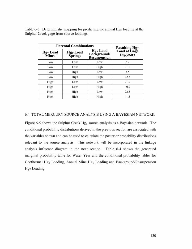
130

Table 6-3. Deterministic mapping for predicting the annual HgT loading at the Sulphur Creek gage from source loadings.

Parental Combinations

HgT Load Mines

HgT Load Springs

HgT Load Background/Resuspension

Resulting HgT Load at Gage

(kg/year)

Low Low Low 2.2 Low Low High 21.2 Low High Low 3.5 Low High High 22.5 High Low Low 21.2 High Low High 40.2 High High Low 22.5 High High High 41.5

6.4 TOTAL MERCURY SOURCE ANALYSIS USING A BAYESIAN NETWORK

Figure 6-5 shows the Sulphur Creek HgT source analysis as a Bayesian network. The

conditional probability distributions derived in the previous section are associated with

the variables shown and can be used to calculate the posterior probability distributions

relevant to the source analysis. This network will be incorporated in the linkage

analysis influence diagram in the next section. Table 6-4 shows the generated

marginal probability table for Water Year and the conditional probability tables for

Geothermal HgT Loading, Annual Mine HgT Loading and Background/Resuspension

HgT Loading.

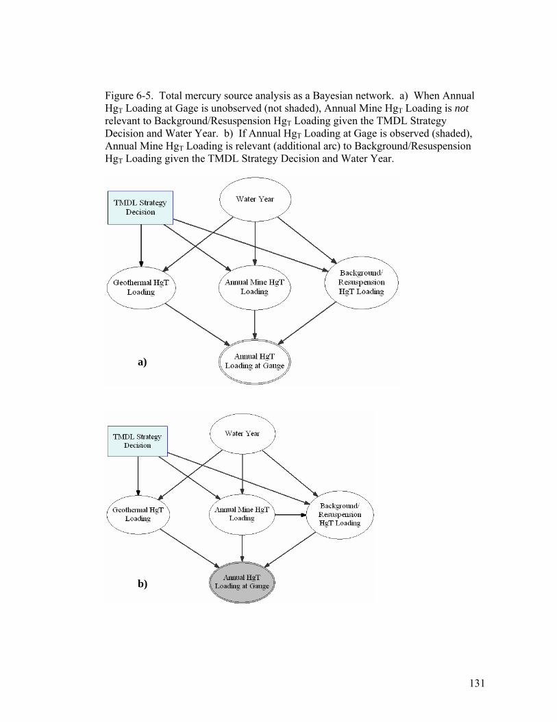
Figure 6-5. Total mercury source analysis as a Bayesian network. a) When Annual HgT Loading at Gage is unobserved (not shaded), Annual Mine HgT Loading is not relevant to Background/Resuspension HgT Loading given the TMDL Strategy Decision and Water Year. b) If Annual HgT Loading at Gage is observed (shaded), Annual Mine HgT Loading is relevant (additional arc) to Background/Resuspension HgT Loading given the TMDL Strategy Decision and Water Year.

a)

b

)

131

132

Table 6-4. Probability tables for source analysis variables.

{Water Year|&} Probability Source

Dry 51 Frequency from data1

Wet 49 Frequency from data1

Probability {Annual Mine HgT Loading|Dry Year} Status

Quo Mine

Strategy Geothermal & Mine Strategy

Source

Low 0.993 0.999 0.993 High 0.007 0.001 0.007

Simulation from published data2, expert judgment

Probability {Annual Mine HgT Loading|Wet Year} Status

Quo Mine


Source

Low 0.54 0.964 0.54 High 0.46 0.036 0.46

Simulation from published data2,3, expert judgment

Probability {Geothermal HgT Loading|Dry Year} Status

Quo Mine


Source

Low 0.81 0.81 1 High 0.19 0.19 0


Probability {Geothermal HgT Loading|Wet Year} Status

Quo Mine


Source

Low 0.51 0.51 0.962 High 0.49 0.49 0.038


Probability {Annual Background/

Resuspension HgT Loading | Dry Year }

Status Quo

Mine Strategy

Geothermal & Mine Strategy

Source

Low 0.89 0.999 0.99999 High 0.11 0.001 1e-005


Probability {Annual Background/

Resuspension HgT Loading | Wet Year }

Status Quo

Mine Strategy


Source

Low 0.21 0.8 0.9 High 0.79 0.2 0.1


Notes: 1) Based on California Department of Water Resources, 1906 – 2004 water year indices for Sacramento Valley: {indices for dry, critical years} = dry and {index for wet years} = wet. 2) Data from RWQCB-CV, 2004b 3) Wet year average load estimate from representative wet year index.

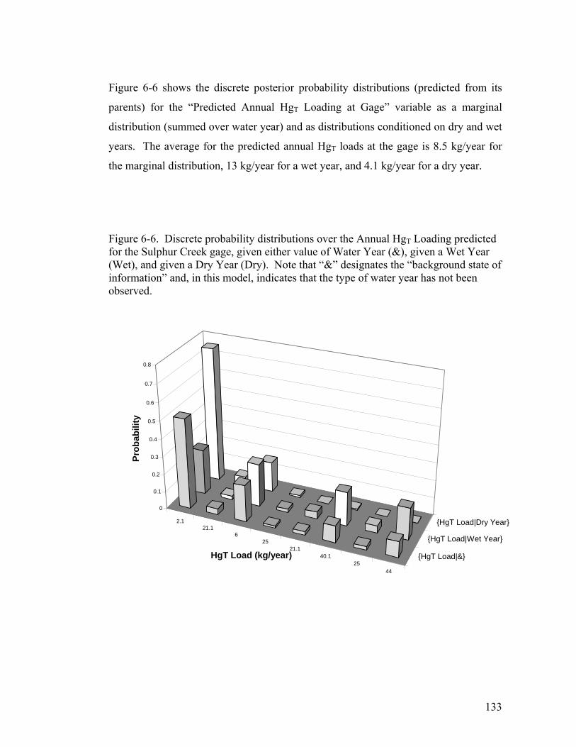
133

Figure 6-6 shows the discrete posterior probability distributions (predicted from its

parents) for the “Predicted Annual HgT Loading at Gage” variable as a marginal

distribution (summed over water year) and as distributions conditioned on dry and wet

years. The average for the predicted annual HgT loads at the gage is 8.5 kg/year for

the marginal distribution, 13 kg/year for a wet year, and 4.1 kg/year for a dry year.

Figure 6-6. Discrete probability distributions over the Annual HgT Loading predicted for the Sulphur Creek gage, given either value of Water Year (&), given a Wet Year (Wet), and given a Dry Year (Dry). Note that “&” designates the “background state of information” and, in this model, indicates that the type of water year has not been observed.

2.121.1

625

21.140.1

2544

{HgT Load|&}

{HgT Load|Wet Year}

{HgT Load|Dry Year}

0

0.1

0.2

0.3

0.4

0.5

0.6

0.7

0.8

Prob

abili

ty

HgT Load (kg/year)

134

6.5 MERCURY TMDL LINKAGE ANALYSIS AS A CAUSAL INFLUENCE

DIAGRAM

MODELING UNCERTAIN CAUSE-AND-EFFECT USING EXPERT ELICITED PROBABILITY

DISTRIBUTIONS

While the uncertainties in current total and methylmercury loading estimates for the

source analysis are significant, largely due to a lack of data, the uncertainties in the

linkage analysis are much larger, and include a lack a data as well as significant gaps

in the understanding of the causal relationships between inorganic mercury loading

and factors that promote the net formation of methylmercury (Benoit et al. 2003;

Calfed Bay-Delta Program 2005; Marvin-DiPasquale et al. 2000; Slotton et al. 2004;

Wiener et al. 2003). Current research suggests that methylmercury may be more of a

“hotspot” problem than an inorganic mercury loading problem. Hotspots are thought

to occur when relevant environmental conditions are optimized for promoting the net

formation of methylmercury. In such conditions, while reactive mercury in sediment

is a necessary factor for the formation of methylmercury, it may rarely be the limiting

factor in many watersheds (Calfed Bay-Delta Program 2005). The environmental

factors that promote the net methylation of mercury are discussed below.

One observation that supports the hotspot view is the strong relationship

between methylmercury concentration and season. In the latter hot period of the dry

season (July and August), when flows are low, temperatures are high, and oxygen

levels are low in water, methylmercury concentrations can be more than 300 times

higher than in the latter part of the wet season (RWQCB-CV 2004b). In the wet

season, observed methylmercury comprises from 0.01% to 0.16% of total mercury. In

the dry season, the range is from 0.03% to 2%. This seasonal hotspot aspect of the

linkage between inorganic mercury loading and local methylmercury concentration

has significant implications for addressing the problem of environmental

methylmercury, but at this time, the appropriate measures to address the problem are

still controversial, even at a site specific level (Calfed Bay-Delta Program 2005).

135

As discussed in more detail below, part of the difficulty in relating total

mercury loading to methylmercury formation is due to a lack of data on the

relationship between total mercury loading, the spatial distribution on the

concentration of total mercury in sediments and erodable materials throughout the

watershed, and the spatial and temporal distributions of reactive mercury in sediment

near the primary zone of mercury methylation in Sulphur Creek, the creekbed

oxic/anoxic sediment interface.

Data limitations and knowledge gaps make the predicted response of seasonal

methylmercury concentrations to changes in total mercury loadings a very difficult

and highly uncertain endeavor. When one also considers the issue of the unknown

contribution of background geothermal mercury sources to the concentration of

reactive mercury in sediment, the uncertainty in the predicted consequences of mine

mitigation efforts becomes enormous (Churchill and Clinkenbeard 2005; Rytuba

2005b). In fact, a first order analysis could be made in which one assumes that the

uncertainty in the resulting future post-mine mitigation methylmercury concentration

trend is independent of the decision to mitigate. In other words, it is arguable that an

appropriate decision model could be made in which future methylmercury

concentrations are an uncertainty that are independent of the mitigation strategy

chosen. Rather than take this approach, the proposed model includes hypotheses in

which mine mitigation may or may not have an effect on the concentrations of reactive

mercury in sediment and methylmercury in the watershed. This preserves the causal

relationship between the potential controls and the desired environmental targets,

while allowing for the very real possibility that methylmercury concentrations are

outside of the feasible control of Sulphur Creek mercury TMDL decision-makers.

While other work (nutrient loading and eutrophication-related water quality

problems) has focused on the using uncertainty analysis on calibrated semi-empirical

models to generate the needed probability distributions for modeling water quality

control decisions as a Bayesian network (Borsuk et al. 2003; Reckhow 1999; Stow et

al. 2003), this work takes a very different approach. Many aspects of the linkage

136

analysis for the nutrient loading-related problem addressed by Borsuk, Reckhow, and

Stow were supported by a relatively large data set and accepted semi-empirical

models. As discussed above, the Sulphur Creek mercury linkage analysis is

comparatively fraught with missing information. Given this situation, the integrated

use of the scant available data and scientific expertise in a probabilistic framework

was determined to be the most useful way to proceed for the mercury TMDL linkage

analysis. Because of the absence of accepted deterministic models, it was also judged

that the best way to integrate the available relevant data (both site-specific and from

other watersheds) was to have the domain experts subjectively consider the data

before expressing their uncertainty in the needed conditional probabilistic

relationships between the variables of interest. Methodologies for reducing bias,

avoiding the introduction of bias, etc., in the elicitation of probability distributions

have been reviewed extensively in the literature (Morgan and Henrion 1990; Spetzler

and von Holstein 1975; Tversky and Kahneman 1974). Experts from Stanford

University (Aaron Slowey) and the U.S. Geological Survey (James J. Rytuba and

Mark Marvin-DiPasquale) were interviewed following a description of the approach

and a review of the available information.

LINKAGE ANALYSIS

Figure 6-7 shows a Bayesian network version of a mercury linkage analysis for the

Sulphur Creek watershed. It predicts the probability distributions over several

variables of interest to decision-makers and scientists: 1) annual median HgT/TSS

concentration in fine grained sediment above the gage (“HgT/TSS”) in response to the

various TMDL mitigation alternatives; 2) median reactive mercury in sediment

(“Hgsed*”) above the gage; 3) annual median methylmercury (“MeHgT”) at the gage;

and 4) MeHgT loading at the gage. Other variables are included in the linkage analysis

to aid in the prediction of these variables of interest, including the hypothesis variable,

“Mine Mitigation Reduces HgT/TSS?”, which has states TRUE and FALSE. FALSE

refers to the outcome in which mine mitigation results in no discernable change in

annual median HgT/TSS because of the high background mercury sources. TRUE

Figure 6-7. TMDL linkage analysis as a Bayesian network relating total mercury loading to environmental targets of interest.

137

138

refers to the outcome in which mine mitigation reduces HgT/TSS during wet season

flows to the regional background level of 1 - 10 ppm. “Percent Reactive HgT” refers

to the fraction of HgT/TSS that contributes to the pool of reactive mercury in sediment.

“Water Season” has states “Wet”, which refers to the rainy season defined as October

1 to March 31, and “Dry”, which refers to the balance of the water year. “Water

year” has the same definition as in the source analysis.

The structure of the model reflects the fact that mercury methylation is

believed to be controlled by the concentration of reactive mercury in sediment

(Hgsed*), as defined in Chapter 5, and the “level of microbial activity” of bacterial

species that methylate reactive mercury in-situ. There is no direct information on the

concentrations of reactive mercury in sediment in Cache Creek. However, some

relevant information is available from mercury methylation potential studies in the

Cache Creek watershed (Bloom 2001; Domagalski et al. 2003; Suchanek et al. 2004)

and studies from other watersheds (Benoit et al. 2003; Marvin-DiPasquale 2005). In

this model, Hgsed* is conditioned by Annual Average Hg/TSS at Gage and Percent

Reactive Hg in HgT/TSS. While the uncertainty in Hgsed* is very large, this structure

suggests that observed Hg/TSS provides relevant information about concentration and

that the source of the mercury (mines/geothermal/soils) provides some limited

information about speciation.

The use of hypothesis variables to describe the effectiveness of mine

mitigation in reducing annual average HgT/TSS (Mine Reduction Reduces HgT/TSS?,

“HgT/TSS reduction hypothesis”) and the percentage of reactive mercury in sediment

(Percent Reactive Hg in Sediment?, “percent reactive mercury hypothesis”) is a

reflection of the fact that both variables will remain unobserved before the decision is

made. While research could do much to inform the HgT/TSS reduction hypothesis,

that variable can not be completely resolved until mine mitigation has been performed

and the remaining contaminated sediment has been partially flushed from the creek.

The percent reactive mercury hypothesis variable could be observed before the

decision is made, but this was determined to be too expensive by decision-makers.

139

The use of hypothesis variables allows decision-makers to consider the decision to

collect more information about these hypotheses in terms of TMDL decision value, the

current state of information, and a consideration of which other variables could also be

observed in the future. This allows much more robust information collection decisions

to be made, formalizing many of the intuitive approaches currently used (Howard

1970).

The state of the “microbial activity” variable can also be thought of as a

hypothesis variable, since it cannot be directly observed. Instead, it should be thought

of as a useful construct that describes the aggregate effect of the many factors that we

partially understand as influencing the efficiency of the microbial methylation of

mercury (Marvin-DiPasquale 2005). For example, it could be modeled as being

conditionally dependent on seasonal sulfate and sulfide concentrations, temperature,

flow conditions, redox conditions, etc. Also, the state of microbial activity can be

updated based on a test set of current or future observations of methylmercury data. It

is in this sense that “microbial activity” can be thought of as a hypothesis variable in a

Bayesian network.

PROBABILITY DISTRIBUTION OVER ANNUAL AVERAGE HGT/TSS AT GAGE

The concentration of total mercury in water (HgT, ng/L) divided by the concentration

of total suspended solids (TSS, mg/L), HgT/TSS (ppm), provides an indicator of the

average concentration of total mercury in suspended and re-suspended sediment

upstream of the point of sample collection. In the following discussion, the annual

average HgT/TSS value observed/predicted at the Sulphur Creek gage will be referred

to as “HgT/TSS”. Figure 6-8 shows the relationship between the sub-model for

HgT/TSS and the sub-model for reactive mercury in sediment.

What is known about the complex relationship between HgT/TSS, flow, and

water season is discussed in Chapter 5. That discussion suggests that the available

water quality and flow data and the available information about mercury sources and

speciation support the use of a seasonal model that uses flow ranges for the wet

140

season. In addition, the potential influence of the mine mitigation and geothermal

spring mitigation alternatives on HgT/TSS is modeled by conditioning HgT/TSS by

the mitigation decision. The large uncertainty in the effects of mine mitigation on

HgT/TSS is modeled by conditioning HgT/TSS on the hypothesis variable, “Mine

Mitigation Reduces HgT/TSS”, as discussed previously. In this hypothesis variable,

FALSE designates the result that mine mitigation does not influence HgT/TSS and

TRUE designates the result that annual average HgT/TSS is reduced towards regional

background levels of 1 – 10 ppm. This approach allows decision-makers to consider

the possibility that mine mitigation may have a negligible impact on HgT/TSS at the

gage due to large background HgT loadings and contaminated sediments (Churchill

and Clinkenbeard 2005; Rytuba 2005a). Reductions in HgT/TSS due to geothermal

spring mitigation were also modeled as resulting in the attainment of regional

background levels. While there is uncertainty that this could be achieved, the

uncertainty is small relative to the uncertainty in the effect of mine mitigation on

HgT/TSS.

For dry season flows, the probability distribution over HgT/TSS for current

conditions (“status quo alternative”) is modeled as a lognormal distribution

independent of flow (n = 8). For wet season flows, HgT/TSS is modeled as two

different lognormal distributions for flows less than (n = 16) and greater than (n = 23)

60 cfs. Table 6-5 summarizes the parameters used for modeling HgT/TSS. The

assumption of population lognormality was checked using the available data for all

season/flow data partitions using normal probability plots (Rice 1995). The

probabilities used to express the uncertainty in the relationship between mitigation and

HgT/TSS conditioned on water season and the HgT/TSS reduction hypothesis are

shown in Table 6-6.

141

Figure 6-8. Sub-model for Annual Average HgT/TSS at Gage and Reactive Mercury in Sediment

142

Table 6-5. Parameters for season/flow dependent HgT/TSS model.

Water Season Flow Range Average1

(± S.E.) Standard Deviation1 (± S.E.)

Dry All 1.4 ± 0.0009 0.25 ± 0.04 Wet Flow < 60 cfs 1.5 ± 0.001 0.43 ± 0.0009 Wet Flow > 60 cfs 0.87 ± 0.0004 0.18 ± 0.0003

Note: Estimated by bootstrapping the available data for that season/flow partition (10,000 iterations). The average and standard deviation refer to the distribution over log(HgT/TSS).

Table 6-6. Probability table for annual average HgT/TSS at gage.

Probability1{Annual Average HgT/TSS at Gage| Mine

Mitigation Reduces HgT/TSS? = False, Dry Season}

StatusQuo

Mine Strategy


Low = 1 ppm 0 0 0.95 Nominal = 10 ppm 0.93 0.93 0.05 High = 100 ppm 0.07 0.07 0

Probability1{Annual Average HgT/TSS at Gage| Mine Mitigation Reduces HgT/TSS? = False, Wet

Season} StatusQuo

Mine Strategy


Low 0 0 0.70 Nominal 0.35 0.35 0.30

High 0.65 0.65 0 Probability1{Annual Average HgT/TSS at Gage| Mine

Mitigation Reduces HgT/TSS? = True, Dry Season}

StatusQuo

Mine Strategy


Low 0 0.50 0.95 Nominal 0.93 0.50 0.05

High 0.07 0 0 Probability1{Annual Average HgT/TSS at Gage| Mine

Mitigation Reduces HgT/TSS? = True, Wet Season}

StatusQuo

Mine Strategy


Low 0 0 0.70 Nominal 0.35 0.77 0.30

High 0.65 0.23 0

Notes: 1) Simulation from published data (RWQCB-CV, 2004b), expert judgment (James J. Rytuba).

143

PROBABILITY DISTRIBUTION OVER ANNUAL MEDIAN REACTIVE MERCURY IN

SEDIMENT UPSTREAM OF GAGE

Reactive mercury in sediment (Hgsed*) is an operationally-defined fraction of total

mercury in sediment that is used as surrogate for the pool of inorganic mercury that is

available for microbial methylation. It is defined more specifically in Chapter 5. The

hypothesis is that this fraction is likely available to microbes for methylation, and thus

represents a surrogate measure of ‘microbially available’ Hg(II). Since there are no

data on Hgsed* in this watershed, a probability distribution based on the available

HgT/TSS data and observations about the fraction of HgT comprised by Hgsed* in other

watersheds was elicited from experts at the U.S. Geological Survey, Dr. James J.

Rytuba and Dr. Mark Marvin-DiPasquale. The 5th , 50th, and 95th percentile values for

the percentage of total mercury in sediment (or its surrogate, HgT/TSS) comprised by

Hgsed* for a wide variety of natural environments are 0.01%, 1%, and 5%, respectively

(Marvin-DiPasquale 2005). Based on the large uncertainties in the mercury speciation

in HgT/TSS and sediment in the Sulphur Creek and Cache Creek watersheds, a

uniform distribution from 0.01% to 5% was used (Bloom 2001; Marvin-DiPasquale

2005; Rytuba 2005c). Table 6-7 presents the probability table for annual median

Hgsed* based on the probability distribution over HgT/TSS, Percent Reactive Mercury

in HgT/TSS, and expert judgment (Rytuba 2005c; Slowey 2005).

PROBABILITY DISTRIBUTION OVER ANNUAL MEDIAN CONCENTRATION OF

METHYLMERCURY IN WATER AT THE GAGE

Table 6-8 shows the probability table for annual median concentration of

methylmercury in water at the gage, elicited from Dr. Mark Marvin-DiPasquale of the

U.S. Geological Survey. The available methylmercury data for Sulphur Creek, Bear

Creek, and Cache Creek were examined by Dr. Marvin-DiPasquale before this

elicitation.

144

Table 6-7. Probability table for annual median reactive mercury in sediment (Hgsed*).

Probability1

{Ann. Median Hgsed* | Ann. Avg HgT/TSS = Low} % Reactive Hg in

Sediment = Low

% Reactive Hg in Sediment =

High Low = 0.0001 ppm 0.999 0.99

High = 5 ppm 0.001 0.01 Probability1

{Ann. Median Hgsed* | Ann. Avg HgT/TSS =

Nominal} % Reactive Hg in Sediment = Low


High Low 0.99 0.90 High 0.01 0.10

Probability1

{Ann. Median Hgsed* | Ann. Avg HgT/TSS = High} % Reactive Hg in

Sediment = Low


High Low 0.90 0.0001 High 0.10 0.9999

Notes: 1) Simulation from published data (RWQCB-CV, 2004b), expert judgment (James J. Rytuba, Aaron Slowey).

Table 6-8. Probability table for annual median concentration of methylmercury in water at the gage (MeHgT).

Probability1

{Ann. Median MeHgT | Hgsed* = Low} Microbial Activity

= Low

Microbial Activity = High

Low = 0.06 ng/L 0.93 0.20 Nominal = 1 ng/L 0.07 0.80

High = 20 ng/L 0 0 Probability1

{Ann. Median MeHgT | Hgsed* = High} Microbial Activity

= Low

Microbial Activity = High

Low 0.05 0 Nominal 0.95 0.06

High 0 0.94 Notes: 1) Simulation from published data (RWQCB-CV, 2004b), expert judgment (Mark Marvin-DiPasquale).

145

PROBABILITY DISTRIBUTION OVER ANNUAL METHYLMERCURY LOADING AT THE GAGE

The probability distribution over methylmercury loading at the Sulphur Creek gage

(MeHgT) was simulated from the available mean daily flow data, using the median

methylmercury concentration in water as the predicted concentration (Table 6-9). As

described in Chapter 5, methylmercury was approximately lognormally distributed

over the period of record, 2000 – 2003. The median value for the period of record was

0.76 ng/L. The mean daily flow data for 2000 – 2003 was used to simulate annual

MeHgT loadings (g/year) and to explore the relationship between annual discharge and

annual MeHgT loading (g/year). Figure 6-9 shows this relationship for the current

estimate of annual median MeHgT value and for assumed values of 0.06, 1.0 and 20

ng/L. As with the annual HgT loading, the simulated MeHgT load for 2001 was used

as the typical dry year. The MeHgT load for the wet year was predicted from the linear

relationships shown in Figure 6-9 using an annual discharge of 1.5 million acre-

feet/year for each value of the annual median methylmercury concentration.

Figure 6-9. Relationship between Sulphur Creek annual discharge and the simulated annual methymercury load (kg/year) using a lognormal distribution for predicted MeHgT, current conditions (status quo strategy). In the legend, “m” refers to the hypothetical mean value of the annual MeHgT distribution.

0.1

1

10

100

0.3 0.5 0.7 0.9 1.1 1.3

Annual Discharge (106 acre-feet/year)

Ann

ual M

eHg T

Loa

d (g

/yea

r)

m = 0.06m = 1m = 20Current Conditions

146

Table 6-9. Probability table for predicted annual methylmercury loading at the gage (g/year).

Probability1

{Ann. MeHgT Load | Ann. Median MeHgT = Low} Water Year = Dry

Water Year = Wet

Low = 0.25 g/year 0.995 0.89 Nominal = 5 g/year 0.005 0.11 High = 100 g/year 0 0

Probability1{Ann. MeHgT Load | Ann. Median MeHgT =

Nominal} Water Year = Dry

Water Year = Wet

Low 0 0 Nominal 0.989 0.89

High 0.011 0.11 Probability1

{Ann. MeHgT Load | Ann. Median MeHgT = High} Water Year = Dry

Water Year = Wet

Low 0 0 Nominal 0.76 0.23

High 0.24 0.77 Notes: 1) Dry year simulation from published data (RWQCB-CV, 2004b) for 2001. Wet year loading distribution estimated from the relationship shown in Figure 6-9.

147

6.6 REFERENCES





Calfed Bay-Delta Program. (2005). "News from the Calfed Bay-Delta Science Program." Calfed.






Hastie, T., Tibshirani, R., and Friedman, J. (2001). The Elements of Statistical Learning: Data Mining, Inference, and Prediction, Springer, New York.


Johnson, D., Miller, A. C., and Rice, T. R. (2002). "Triangular Approximations for Continuous Random Variables in Risk Analysis

Discrete Approximations of Probability Distributions." Journal of the Operational Research Society, 53(4), 457-467.


Marvin-DiPasquale, M., Agee, J., McGowan, C., Oremland, R. S., Thomas, M., Krabbenhoft, D., and Gilmour, C. C. (2000). "Methyl-Mercury Degradation

148

Pathways: A Comparison among Three Mercury-Impacted Ecosystems." Environmental Science & Technology, 34(23), 4908 - 4916.

Miller, A. C., and Rice, T. R. (1983). "Discrete Approximations of Probability Distributions." Management Science, INFORMS: Institute for Operations Research, 352.


Poland, B. (1996). "Discretizing Probability Distributions to Two or Three Points by Matching Moments." 6.


Rice, J. A. (1995). Mathematical Statistics and Data Analysis, Duxbury Press, Belmont, CA.





Rytuba, J. J. (2005c). "Reactive mercury in sediment as a percentage of HgT/TSS." Menlo Park, CA, Personal Communication to William Labiosa.


Slowey, A. (2005). "Speciation of reactive mercury in sediment." Stanford, CA. Smith, J. E. (1993). "Moment Methods for Decision Analysis." Management Science,

39(3), 340-358. Spetzler, C. S., and von Holstein, S. l. (1975). "Probability Encoding in Decision

Analysis." Management Science, 22(3). Stow, C. A., Borsuk, M. E., and Reckhow, K. H. (2003). "Comparison of estuarine

water quality models for TMDL development in the Neuse River Estuary." Journal of Water Resources Planning and Management, 129, 307-314.


Tversky, A., and Kahneman, D. (1974). "Judgment Under Uncertainty: Heuristics and Biases." Science, 185, 1124-1131.

149

Wiener, J. G., Krabbenhoft, D. P., Heinz, G. H., and Scheuhammer, A. M. (2003). "Ecotoxicology of Mercury." Handbook of Ecotoxicology, B. A. R. G. A. B. J. J. C. David J. Hoffman, Jr., ed., Lewis Publishers, Boca Raton, 409-463.

Williams, T. M. (1992). "Practical Use of Distributions in Network Analysis." Journal of the Operational Research Society, 43(3), 265-270.

150

CHAPTER 7: SULPHUR CREEK MERCURY TMDL DECISION ANALYSIS

This chapter demonstrates the use of the proposed decision analytical approach for

TMDL setting. While the level of collaboration with the decision-makers for this case

study was not adequate to perform a real-world decision analysis, the intent of this

chapter is to demonstrate the proposed decision analytical approach. For the

purposes of this demonstration, we assume that our somewhat fictionalized decision

participants have fully cooperated in the creation of the conceptual decision model

presented in Chapter 5, trust the expertise encoded in the probability distributions

presented in Chapter 6, and agree that the valuation approach (presented below)

reflects their preferences. The proposed decision analytical methodology is intended

to be adaptable to a real-world TMDL decision-making situation in collaboration with

decision-makers and stakeholders, taking into consideration data limitations,

knowledge gaps, tight regulatory deadlines, and limited budgets for information

collection and modeling.

For this demonstration, I develop and describe a parametric value model that

does not require consensus on the desirability of compliance with the various TMDL

targets. The approach is designed for use in stakeholder situations in which

participants are cooperative, but do not necessarily share the same preferences. This

value model is incorporated into a decision model that builds on the mercury

mitigation Bayesian network explicated in Chapters 5 and 6.

Decision analytical results from this fully-specified decision model are

presented and interpreted. Contingent on the value of non-compliance (as defined

below), best strategies are determined, sensitivity to key assumptions and probabilities

are evaluated, and the value of clairvoyance (perfect information) for key uncertainties

are presented. The decision analytical approach and types of insights generated serve

as an example useful for transferring the approach to other TMDL situations.

151

7.1 MITIGATION COSTS AND NON-COMPLIANCE PENALTIES: A

PARAMETRIC VALUE MODEL

Figure 7-1 shows the Sulphur Creek TMDL decision as an influence diagram with a

multi-attribute value model27 defined as the sum of the expected mitigation cost and

non-compliance penalties28 for a particular strategy. Here, “non-compliance” is in

reference to two TMDL regulatory targets, the total mercury loading and total

methylmercury loading exported from Sulphur Creek to lower Bear Creek. The total

mercury load target can be thought of as a “downstream issue”, in that it potentially

affects methylmercury concentrations in water and fish downstream (e.g., in the San

Francisco Bay delta). The methylmercury load target is more of a “local issue”, in that

potentially affects methylmercury concentrations immediately downstream in Lower

Bear Creek. The variables shown in the model (Figure 7-1) are defined in Chapter 5

and their associated probability tables are presented in Chapter 6. The use of penalty

functions in optimization problems like this is standard methodology (Bertsimas and

Tsitsiklis 1997; Sundaram 1996).

27 Multi-attribute value models are defined in Chapter 4. In brief, they can be thought of as a bundle of

endpoints or targets that decision-makers are interested in for a particular decision. 28 In decision analysis, a “penalty function” is a tool that can be used to constrain targeted variables for

the purposes of exploring the trade-offs between the risk of violating targets and the costs expended in lowering this risk. In this context, a penalty does not refer to a legal fine that will be imposed upon the decision-makers by a regulatory agency, but rather reflects the social cost of violating the target.

1

52

Figure 7-1. Influence diagram for Sulphur Creek mercury TMDL.

153

The Bayesian network in Figure 7-1 calculates the posterior probabilities of non-

compliance conditioned on TMDL mitigation strategy, which is defined as the

probability of non-compliance (pNC,Ti) for target Ti given all prior data, current

scientific understanding, and available expertise about the effects of the various

mitigation strategies. The value of the penalty for non-compliance with target Ti is

calculated as theproduct of the cost associated with being in the state of non-

compliance (CNC,Ti) and the probability of non-compliance with Ti (pNC,Ti):

)17(* ,,, −= EquationCpPenalty TiNCTiNCTiNC .

In the case of a single decision-maker, the value of CNC,Ti could be elicited as a unique

value. However, in the case of a social decision, the meaning of CNC,Ti is much more

complicated, although one could interpret it as the social disbenefit of non-compliance

with regulatory target Ti. Such a social disbenefit (or cost) would have a highly

uncertain value that could be estimated through a variety of benefit estimation

methodologies (observed behavior, surveys, secondary sources, etc.) (Boardman et al.

2001; Heathcote 1998). However, in this work, the value of CNC,Ti is parameterized to

evaluate its effect on the identification of the best strategy. This method provides very

useful information to decision-makers without the requirement for consensus on

preferences. Since the identified best strategy is always contingent on CNC,Ti, the

approach adopted could be described as “decision analytical support” rather than

“decision analysis”, since an optimal strategy is not uniquely identified.

The mitigation costs for the mine strategy and the status quo are loosely based

on estimates from documents supporting the Sulphur Creek TMDL (RWQCB-CV

2004b; Tetra Tech 2003), but the geothermal & mine strategy mitigation cost is simply

assumed to be twice the mine strategy mitigation cost. Note that the purpose of the

analysis is to illustrate the Bayesian network-based decision analytical approach and

that, while the actual numbers used are reasonable, they do not reflect the beliefs of

the actual decision-makers. Table 7-1 summarizes the mitigation costs used and a

brief description for each strategy.

154

Table 7-1. Mitigation costs used in the decision analysis.

Alternative Mitigation Cost Notes1

Status quo $500,0001Educational programs to educate downstream fish consumers, other social controls

Mine strategy $3,350,0001 Targeted mine waste removal, erosion control at mine sites in watershed

Geothermal &

mine strategy $6,700,0002 High priority mine waste removal, erosion

control, and geothermal spring mitigation.

1. (Delta Tribunal Mercury Council 2005).

2. Chosen as twice the mine strategy mitigation cost.

7.2 FULLY-SPECIFIED SULPHUR CREEK TMDL INFLUENCE DIAGRAM

Appendix A shows the posterior distributions for all variables for each alternative:

status quo, mine strategy, and geothermal & mine strategy. Figure 7-2 shows the

posterior distributions for current conditions (status quo alternative) calculated by an

implementation of the model in the GeNIe 2.0 Bayesian network programming

environment (Decisions Systems Laboratory 2005). This fully specified model is used

to determine best strategies conditioned on the value of CNC,Ti (Section 7.4), to

perform sensitivity analysis on key uncertainties (Section 7.5), and to determine the

value of clairvoyance on these uncertainties (Section 7.6). But first, the total mercury

and methylmercury loadings predicted by this model are reported by strategy and

water year in Section 7.3.

155

7.3 PREDICTED TOTAL AND METHYLMERCURY LOADINGS BY

STRATEGY

The posterior probability distributions over the predicted long-term total mercury

(HgT) loading (Figure 7-3) and the methylmercury loading (Figure 7-4) for each

strategy were calculated using the Bayesian network from Figure 7-1. The predicted

long-term total HgT and MeHgT loadings for each TMDL strategy, given dry, wet, and

any water year are tabulated (Table 7-2). In the case of post-mitigation predictions,

“long- term” refers to the new steady state loadings that are predicted to result on the

time-scale of years to decades after mitigation. In the case of the status quo, there is

no prediction time lag. Table 7-2 also shows the credibility of compliance (COC) with

the HgT loading and MeHgT loading targets for each strategy. In this model, the

COCHgT is defined as the posterior probability that the annual HgT loading at the gage

is in state “LLL”, which refers to the situation where the annual mine HgT loading,

annual geothermal HgT loading, and annual background/resuspension HgT loading are

all in the state “Low”. COCMeHgT similarly refers to the posterior probability that the

annual MeHgT loading at the gage is in the state “Low”. Other definitions of the

credibility of compliance are possible. For example, treating the loadings as

continuous variables, COCHgT could be defined as the cumulative distribution for

{HgT Load ≤ Target}. However, for simplicity of presentation and given the very

large uncertainties in the predicted loadings, a discrete representation with targets

defined explicitly as states is adequate.

1

56

Figure 7-2. Posterior distributions over all variables given no mitigation (status quo strategy).

Probabilties

Key

States

Name

Figure 7-3. Posterior distribution over predicted long-term annual HgT loading at gage by strategy.

2.1 21.1 6 25 21.1 40.1 25 44

Mine strategy

Geothermal & mine Strategy

Status quo00.10.20.3

0.4

0.5

0.6

0.7

0.8

Prob

abili

ty

HgT Load (kg/year)

Mine strategy Geothermal & mine Strategy Status quo

157

1

58

Figure 7-4. Posterior distribution over predicted long-term annual MeHgT loading at gage by strategy.

0.25 5 100

Mine strategy

Geothermal & mine strategy

Status quo

0

0.1

0.2

0.3

0.4

0.5

0.6

0.7

Prob

abili

ty

MeHgT Load (g/year)

Mine strategy Geothermal & mine strategy Status quo

159

Table 7-2. Predicted annual HgT and MeHgT loadings at the Sulphur Creek gage and the associated credibility of compiance (COC), by strategy and water year.

Mine Strategy Geothermal & Mine Strategy Status Quo

Annual Loading | &1

Average HgT Loading

(kg/year), COC2 4.8, COC = 0.64 11, COC = 0.71 12, COC =

0.52

Average MeHgT Loading

(g/year), COC 11, COC = 0.33 6.3, COC = 0.43

11, COC =

0.31

Annual Loading | Dry Year

HgT Loading (kg/year),

COC2 3.7, COC = 0.79 3.5, COC = 0.93 4.2, COC =

0.77

MeHgT Loading (g/year),

COC 5.8, COC = 0.34 3.5, COC = 0.46

6.1, COC =

0.33

Annual Loading | Wet Year

HgT Loading (kg/year),

COC2 5.9, COC = 0.49 19, COC = 0.48 21, COC =

0.27

MeHgT Loading (g/year),

COC 16, COC = 0.31 9.2, COC = 0.41

17, COC =

0.29

Notes: 1) “&” designates the “background state of information”. In this case, this means that the loading prediction includes the uncertainty about the future state of the water year.

2) Credibility of compliance, defined as the posterior probability that the compliance target is met.

7.4 DETERMINING THE BEST STRATEGY

Using the model shown in Figure 7-2, a best strategy can be determined for the

background state of information contingent on the non-compliance costs, CNC,HgT and

160

CNC,MeHgT. When the non-compliance costs are assigned values, a best strategy is

determined from the expectation of the value model, E[Mitigation Cost + Penalty].

There are several exact and approximate algorithms used for solving influence

diagrams (Jensen 2001; Pearl 1988; Shachter 1986). The computational requirements

for solving a particular probabilistic problem using a given algorithm can be estimated

beforehand. When exact algorithms are predicted to consume an unreasonable amount

of computational resources (storage and/or time), approximation algorithms (e.g.,

stochastic simulation) can be used. For this work, the clustering algorithm29 was used

in the GeNIe 2.0 environment, which provides an exact solution for belief updating

and is feasible for relatively small models (Decisions Systems Laboratory 2005). The

“policy evaluation” mode was used to solve influence diagrams, which is an

implementation of the algorithm proposed by Cooper (Cooper 1988). The policy

evaluation algorithm solves the influence diagram by transforming it into a Bayesian

network and then determining the expected utility for each of strategy. The algorithm

can be computationally intensive for large influence diagrams, but is very fast for the

model shown in Figure 7-2. See Shachter (1986), Jensen (2001), and Pearl (1988) for

further discussion on the details and trade-offs among the various Bayesian network

and influence diagram solution algorithms.

29 The clustering algorithm often uses a two phase process. First, the directed acyclic graph (DAG) is

compiled into a junction tree. Then, probability updating is performed in the junction tree representation. However, the compilation phase is not necessary for many models. The clustering algorithm in GeNIe 2.0 does not use a compilation phase. For more information on the details of the clustering algorithm and other exact algorithms, see Jensen (2001) and Pearl (1988).

161

Figure 7-5 shows the best strategy regions given the values of the non-

compliance social cost parameters (CNC,HgT and CNC,MeHgT), ranging from $ 0 to $

50,000,000. This figure can also be thought of as an analysis of the decision

sensitivity to the non-compliance social cost parameters, in the sense that any

particular combination of CNC,HgT and CNC,MeHgT values uniquely determines an

optimal decision, given those values. Performing a standard decision sensitivity

analysis on CNC,HgT and CNC,MeHgT is then equivalent to treating CNC,HgT and CNC,MeHgT

as unknown parameters. Note from Figure 7-5 that there are regions in which each of

the three alternatives is the best strategy. This suggests that decision-makers should

carefully evaluate where they think they are in terms of this “non-compliance cost

map”. As will be seen, the cost of non-compliance is one of the most important

factors for decision-makers to consider in making this decision. In the actual Sulphur

Creek TMDL decision situation, this factor is only implicitly considered (RWQCB-

CV 2004b). The fact that the real world decision-makers will probably choose either

the mine strategy or geothermal & mine strategy reveals that their cost of non-

compliance values are in either area “1” or “2” of Figure 7-5.

1

62

1

2

3

CN

C,M

eHgT

CNC,HgTx 107 $

x 107 $

Figure 7-5 . Best strategy contigent on CNC,HgT and CNC,MeHgT. Labeled areas denote the best strategy for regions of CNC,HgT , CNC,MeHgT

163

7.5 SENSITIVITY ANALYSIS

The influence diagram implementation can be used to perform sensitivity analysis in a

simple manner by adding a “sensitivity variable” to the model from Figure 7-2. Figure

7-6 demonstrates this method for performing sensitivity analysis using the variable

“Percent Reactive Hg in HgT/TSS” (PRHg). A conditioning arc is added from the

sensitivity variable to the variable of interest and an informational arc is added from

the sensitivity variable (PRHg) to the decision variable (TMDL Strategy Decision).

The sensitivity variable has states “Low”, “Nominal”, and “High”, assumed to have a

uniform marginal distribution. The PRHg is no longer marginal and is now described

by the probability table (Table 7-3):

Table 7-3. Probability table over the sensitivity variable.

Sensitivity States → Percent Reactive Hg

in HgT/TSS

States ↓

Low Case Nominal

Case High Case

Low 0.1 0.5 0.9

High 0.9 0.5 0.1

The nominal case (Sensitivity state = Nominal) is the uniform distribution over the

PRHg variable. The low case has a probability of 0.1 for the PRHg variable having a

state of Low (PRHg = Low) and the high case has a probability of 0.9 for PRHg =

Low. This reduces the sensitivity analysis to solving the influence diagram for the

expected value for the TMDL Strategy Decision variable now that it is conditioned by

the sensitivity variable. Table 7-4 shows that results of the sensitivity analysis for the

1

64

Figure 7-6. Sensitivity to the probability distribution over percent reactive Hg in HgT/TSS.

165

Table 7-4. Sensitivity analytical results for the Percent Reactive Hg in HgT/TSS (PRHg) variable. The value for the best strategy is shown in bold for each state of the sensitivity variable. The values shown are the expected costs (mitigation cost + penalties) for each strategy, given the effect of sweeping through the probability distribution for the PRHg variable on the credibility of compliance, calculated using the Bayesian network model. The mitigation costs used are from Table 7-1 and the assumed values for the social costs of non-compliance for the HgT and MeHgT load targets (CNC,HgT , CNC,MeHgT) are each $30,000,000.

PRHg variable assuming that CNC,HgT = CNC,MeHgT = $30,000,000. The fact that the

best strategy is “Spring Mitigation” for the low and nominal states and the “Mine

strategy” for the high state indicates potential value to gathering information on this

variable, given the assumed values of CNC,HgT and CNC,MeHgT. By varying CNC,HgT and

CNC,MeHgT and repeating this procedure, sensitivity to probability for the PRHg

variable can be explored without assuming particular non-compliance costs.

Figure 7-7 shows a model for performing sensitivity analysis on the Microbial

Activity variable from the model shown in Figure 7-2. Using the procedure just

described and again assuming that CNC,HgT = CNC,MeHgT = $30,000,000, it turns out that

the best strategy is “geothermal & mine strategy” for all states of the sensitivity

variable. For the assumed non-compliance costs, this implies that there is no value to

gathering more information on this variable. This procedure demonstrates the use of

sensitivity analysis as a tool for exploring which uncertainties are most important for

supporting the TMDL decision. Determining which uncertainties have the potential to

Sensitivity States → Low Nominal High

Expected Value of the Decision ↓ ↓ ↓ Mine strategy -$35,464,000 -$33,637,000 -$31,809,000

Geothermal & mine strategy -$32,500,000 -$32,359,000 -$32,218,000

Status quo -$38,011,000 -$35,478,000 -$32,945,000

1

66

Figure 7-7. Sensitivity to the probability of Microbial Activity = Low.

167

change the best strategy to prioritize future information collection activities is a

potentially important application for the proposed decision analytical approach.

While this procedure could again be repeated for a range of non-compliance costs to

map out regions in which the best strategy changes, there are easier methods for

exploring the value of perfect information using influence diagrams, as described in

the next section.

7.6 VALUE OF CLAIRVOYANCE (PERFECT INFORMATION)

The influence diagram implementation of the model shown in Figure 7-2 can be

directly used to calculate the value of clairvoyance (VOC) for the variables in the

model. The value of clairvoyance is based on the abstraction of the “clairvoyant”,

which is a convenient fictional character that omnisciently knows the future outcome

of any decision, but cannot change that future. For the clairvoyant to be able to

answer a query about a future outcome, the possible decision outcomes be clearly

defined in terms of unambiguous events30. The clairvoyant cannot tell you, even in

theory, anything about your preferences, but could tell you exactly how a particular

uncertainty will be resolved in the post-decision future. For outcomes that can be

valued in terms of money, this useful abstraction allows us to formulate the idea of

the value of clairvoyance (perfect information), which serves as the upper limit to the

value of any information gathering activity (Clemen et al. 1996; Howard 1996;

Howard et al. 1972).

Clairvoyance (knowing the future state of an uncertain variable before the

decision is made) can be expressed using the notation of influence diagrams. In this

notation, clairvoyance on an uncertainty is equivalent to the presence of an

informational arc from that uncertainty to the decision variable, which denotes that

its state is known before the decision is made. This is semantically equivalent to

flipping the decision tree described by an influence diagram such that the uncertainty

in question precedes the decision variable in the tree. Since we do not know what the

30 In other words, the events must be mutually exclusive and collectively exhaustive.

168

hypothetical clairvoyant would reveal beforehand, the probability distribution over

the Clairvoyant’s response is the same as the marginal distribution over the

uncertainty. In essence, this allows us to explore whether or not perfect information

would change the best strategy and, for monetized outcomes, allows us to calculate

what that perfect information would be worth to us before the decision is made.

Assuming that the decision-maker is risk neutral, the value of clairvoyance is simply

the difference of the value of the decision31 with clairvoyance and without

clairvoyance (Clemen et al. 1996; Howard 1996). This work assumes risk neutrality

over monetized outcomes, which is appropriate for many public decisions

(Merkhofer 1987). A detailed introduction to the value of clairvoyance can be found

in an introductory decision analysis text, e.g., Clemen (1996) or Howard (1996).

The GeNIe Bayesian network programming environment allows the value of

clairvoyance to be easily calculated for an influence diagram for a risk neutral

decision-maker, automating the steps of comparing the decision value with and

without clairvoyance. Figure 7-8 shows the joint value of clairvoyance on Percent

Reactive Hg in HgT/TSS (PRHg) and Microbial Activity (MA) for several

combinations of CNC,HgT = CNC,MeHgT. These two variables were not picked

haphazardly. They are the only uncertainties with significant VOC over the range of

non-compliance costs. This means that collecting information on these uncertainties

could potentially change the choice of strategy, while collecting information on the

31 In this case study, the “value of the decision” is the expected value of the best strategy. This

corresponds to the strategy with the minimum cost function (mitigation cost + penalties). For at least one of the clairvoyant’s responses, the best strategy changes from the best strategy without clairvoyance. This potential change generates value for the decision with clairvoyance.

Figure 7-8 . Joint value of clairvoyance (VOC) on microbial activity and percent reactive mercury in HgT/TSS as a function of the cost of non-compliance with the HgT load (CNC,HgT) and the MeHgT load (CNC,MeHgT).

Joint VOC, x 103 $

CNC, HgT

CN

C,M

eHgT

7 $

169

x 10

x 107 $

170

other uncertainties will not change the best strategy for a given set of non-compliance

costs.

Joint VOC refers to perfect information on more than one uncertainty

simultaneously and is calculated as the difference between the decision value with

perfect information on the set of uncertainties and without this information. Note that

the joint VOC on two or more variables does not have to be the sum of the VOC on

the individual uncertainties. In fact, two variables with zero VOC can jointly have a

significant VOC, indicating that the clairvoyance on both variables may change the

best strategy while clairvoyance on each individual variable never changes the best

strategy. For example, when CNC,HgT = CNC,MeHgT = $10,000,000, the individual VOCs

on the PRHg and MA variables are zero, but the joint VOC is $176,000. Figure 7-8

also shows that the joint VOC varies considerably depending on the particular values

of CNC,HgT /CNC,MeHgT. This suggests that exploring the magnitude of non-compliance

costs would be also be useful to decision-makers for its implications regarding the

value of clairvoyance on Percent Reactive Hg in HgT/TSS and Microbial Activity.

7.7 SUMMARY

This chapter presents the decision analytical results for the Sulphur Creek mercury

TMDL strategy decision using the Bayesian network (influence diagram) model

created in Chapters 5 and 6. It presents a parametric value model based on the

unknown social costs of non-compliance with two TMDL targets. The model was

designed such that it does not require consensus among decision-makers and

stakeholders. This approach allows decision-makers to separate the importance of

scientific uncertainties from the importance of preferences over possible decision

outcomes. Best strategies are shown as a function of the social costs of non-

compliance with the total mercury (HgT) and methylmercury (MeHgT) load targets

through the use of “decision maps”. Sensitivity analysis is used to demonstrate which

uncertainties are most important for TMDL decision support. For choosing between a

“mine mitigation strategy” and a “geothermal and mine mitigation strategy”, only

171

studies concerning the percent reactive mercury in HgT/TSS from mine run-off versus

geothermal springs and the ability to model microbial activity (related to mercury

methylation efficiency) should be conducted. Value of perfect information analysis is

used to determine the upper limit on money spent for future decision support

information collection activities. A value of perfect information map is also provided

as a function of the social costs of non-compliance with the HgT and MeHgT load

targets. This demonstration is meant to show the capabilities of a decision analytical

approach for identifying and exploring important scientific uncertainties in a complex

TMDL decision problem, to separate informational concerns from value judgments,

and to prioritize information collection activies to support the TMDL decision-making

process.

172

7.8 REFERENCES

Bertsimas, D., and Tsitsiklis, J. N. (1997). Introduction to Linear Optimization, Athena Scientific, Blemont, MA.

Boardman, A. E., Greenberg, D. H., Vining, A. R., and Weimer, D. L. (2001). "Cost-Benefit Analysis: Concepts and Practice." Prentice Hall, Inc., Upper Saddle River, NJ, 526.

Clemen, R. T., DeMonsabert, Sharon, Snyder, Frank, and Shultzaberger, L. (1996). "Making Hard Decisions, An Introduction to Decision Analysis

Comparative Evaluation of Analytical and Intuitive Decision-making." Journal of Management in Engineering, 19(2), 664.

Cooper, G. F. "A Method for Using Belief Networks as Influence Diagrams." Minneapolis, Minnesota, 55-63.

Decisions Systems Laboratory. (2005). "GeNIe (Graphical Network Interface) Software Package." University of Pittsburgh, Department of Information Science and Telecommunications, Pittsburgh, PA.

Delta Tribunal Mercury Council. (2005). "May 5, 2005 Meeting Summary." Woodland, CA.

Heathcote, I. W. (1998). Integrated Watershed Management : Principles and Practice, Wiley, New York.

Howard, R. A. (1996). "Foundations of Decision Analysis." Unpublished Course Reader, Stanford, CA.

Howard, R. A., Matheson, J. E., and North, D. W. (1972). "The Decision to Seed Hurricanes." Science, 176(4040), 1191-1201.

Jensen, F. V. (2001). Bayesian Networks and Decision Graphs, Springer-Verlag, New York.

Merkhofer, M. W. (1987). Decision Science and Social Risk Management, D. Reidel Publishing Co., Boston.

Ortolano, L. (1997). "Environmental Regulation and Impact Assessment." John Wiley & Sons, Inc., New York, 604.


RWQCB-CV. (2004). "Sulphur Creek TMDL for Mercury Draft Staff Report." California Regional Water Quality Control Board, Central Valley Region, 76.

Shachter, R. D. (1986). "Evaluating Influence Diagrams." Operations Research, 34(6), 871-882.

Sundaram, R. K. (1996). A First Course in Optimization Theory, Cambridge University Press, New York.

Tetra Tech. (2003). "Final Engineering Evaluation and Cost Analysis for the Sulphur Creek Mining District, Colusa and Lake Counties, California." CALFED, 393.

173

CHAPTER 8: CONCLUSIONS AND SUGGESTIONS FOR FUTURE RESEARCH

8.1 SUMMARY

The typical current approach to the complexities and uncertainties surrounding TMDL

decision-making is to build deterministic predictive models that characterize the

situation as well as possible and then depend heavily on these models to help make

and support decisions. Uncertainty is currently handled through the use of ad hoc

methods for “doing away” with uncertainty by adopting conservative TMDL targets

(margins of safety) and/or employing conservative modeling choices. The recognition

that TMDL uncertainties are much larger than deterministic thinking warrants is

reflected in the wide adoption of adaptive management as the planning framework.

Answering the question of “how conservative should we be” should be approached by

thinking carefully and strategically about the uncertainties involved and the values at

stake.

To address this problem, this research has a re-framed a real-world mercury

TMDL decision problem from a decision analytical perspective. This paradigm shift

introduces concepts and modes of thinking not currently used in TMDL decision-

making, including outcome-based strategy evaluation, value of clairvoyance (perfect

information), and the explicit separation of scientific uncertainty from decision-maker

preferences. It also provides a formal context for considering the importance of

uncertainty in TMDL decisions, for prioritizing information collecting activities, and

for considering and representing hypotheses within a TMDL decision-modeling

framework. Very importantly, the Bayesian perspective of decision analysis allows

decision participants to interpret new information (monitoring and knowledge) in light

of previous information and knowledge. The proposed decision model frames the

TMDL setting process as a set of related regulatory (scientific, engineering, and

economic) decisions that may involve large uncertainties (limited data bases and

incomplete knowledge) subject to tight regulatory deadlines and small decision

174

process budgets. Poor TMDL decisions avoid the hard work of considering trade-offs

between scientific uncertainties and decision-maker values, which may result in a

higher risk of a bad future outcome. An example of a poor TMDL decision would be

the choice of a strategy that has both high expected compliance costs and a low

probability of achieving compliance within the desired time-frame. Current TMDL

decision-making only considers such possible outcomes implicitly using deterministic

models and margins of safety to “ensure compliance”. In many TMDL situations,

including the mercury TMDL case study used in this research, compliance is not a

certainty for feasible mitigation strategies. Good TMDL decision-making explicitly

considers the important (and often large) uncertainties that may be the difference

between “success” and “failure” for a strategy, recognizes differing decision

participant preferences over possible outcomes, and considers the trade-offs between

the uncertainty of meeting targets and the costs associated with compliance for a

strategy. Ultimately, a good TMDL decision should result in a better chance of

achieving the successful restoration of a water body’s beneficial use at a socially

acceptable cost. From the decision analytical perspective, a good outcome happens to

the lucky decision-maker. A good decision is the result of the quality of the processes

used by decision participants to define and analyze the decision problem.

This research has resulted in a decision model that represents the current

understanding of the uncertain relationships between potential mercury TMDL

mitigation strategies and the environmental targets of interest, total mercury and

methylmercury loads exported from a small mine-impacted Northern California

watershed (Chapter 2). These complex relationships are broken down into

probabilistic causal relationships between variables, in which each variable has an

associated conditional probability table that describes the probability distribution over

its value conditioned on the values of its parent32 variables (Chapters 3 and 5). The

32 As described in Chapter 3, causally related variables can be thought of in terms of structural

equations, in which a child variable (C) is predicted from the states of its various parent variables (Pa(C)). The exact states of the parent variables may themselves be uncertain and the value of the child variable given the exact states of its parents may also be uncertain (random error, ε). This can be represented by: C = F(Pa(C), ε), where F is a function that predicts C from the states of its

175

purpose of the model is to generate posterior probabilities that the targets of interest

will be met in the future, given a particular mitigation strategy (Chapters 5, 6, and 7).

The value of the strategy is modeled as a simple net benefits model (Chapter 7):

where the penalty33 for violating a particular target is modeled as the product of the

posterior probability that the target “i” will be violated (pNC,Ti) and the social cost of

non-compliance with target “i” (CNC,Ti). To avoid the need for decision participant

consensus on the value of the social cost of non-compliance, CNC,Ti is treated as a

parameter. This approach allows the decision participants to explore pair-wise value

trade-offs between targets, to explore the sensitivity of the best strategy to important

informational uncertainties, and to estimate the upper-limit of the value of collecting

new information before the decision is made (Chapters 4 and 7).

Contrary to typical water quality model development practice, the purpose of

the water quality sub-model is not to replace less realistic models, but rather to

provide an alternative causal modeling framework specifically designed for decision

support. In addition to providing a causal understanding of a complex environmental

system, modeling for decision support should provide decision-makers with an

understanding of the meaning of predictive uncertainty in the context of the decisions

being made and in terms useful to decision-makers (Chapters 1, 4, and 7). This

obviously goes beyond the purposes and methods of traditional water quality modeling

and potentially enters into the many sub-fields that make use of results from the

decision sciences, including “decision support”, decision analysis, multi-criteria

decision-making, multi-attribute utility analysis, etc. In short, the burden becomes

),18( −+= EquationPenaltiesCostStrategyValueStrategy

parents, Pa(C). The uncertainty in this functional relationship is represented by the random error term, ε. See Pearl (2000) for a detailed explication of causal networks and structural equation models.

33 In decision analysis, a “penalty function” is a tool that can be used to constrain targeted variables for the purposes of exploring the trade-offs between violating targets and expending resources to meet them. In this context, a penalty does not refer to a legal fine that will be imposed upon the decision-makers by a regulatory agency, but rather reflects the “cost” of violating the target to the decision-participants.

176

scientific modeling for decision support in the face of both significant informational

uncertainty and disputes over preferences and values.

This dissertation proposes an approach for meeting the needs of decision-

makers, while faithfully representing what is currently known about the behavior of a

complex environmental system subject to possible interventions, given the available

data, models, and expert judgment. The approach is based on the use of influence

diagrams, since this tool allows probabilistic modeling of complicated knowledge

systems in the context of decision-making and can be used to perform the full range of

decision analysis. The approach also addresses the complex institutional aspect of

group decision-making by using a parametric penalty value model to model decision-

maker preferences, without requiring consensus. This results in a methodology that

could be described as “decision analytical support” rather than decision analysis, since

best strategies are contingent on the penalty parameter and hence are not uniquely

identified. In essence, this maps out the “decision space” along the dimensions of

social costs on targets of interest to decision-makers.

This research presents a decision analytical approach for handling uncertainty

and balancing trade-offs in a mercury TMDL decision situation. Current decision-

making based on the highly uncertain results from deterministic models of complex

systems makes use of potentially flawed heuristics, subject to many potential errors.

By using a conservative deterministic approach, decision-makers cannot determine

whether they are being overly conservative or not conservative enough. Just as

importantly, by not explicitly separating values and preferences from information

about scientific uncertainty, a conservative deterministic approach avoids the

important question, “conservative for whom?”. The trade-off framework presented in

Chapter 7 explicitly separates these dimensions and allows decision-makers to

consider the importance of scientific uncertainty separately from the importance of

differing stakeholder preferences.

177

8.2 CONCLUSIONS AND MAJOR FINDINGS FOR MERCURY TMDL CASE

STUDY

• The Regional Water Quality Control Board staff should focus their future

Suphur Creek mercury TMDL data collection efforts on identifying and

modeling zones of high microbial activity for mercury methylation and on

characterizing the reactive34 fractions of mercury inputs from mine-related run-

off and geothermal springs (Chapter 7, Section 6). Figure 7-8 could be used by

decision-makers to estimate the upper limit on collecting data on these two

uncertainties. It is important to note that this upper limit depends on the social

costs of non-compliance for the total mercury and methylmercury TMDL

targets.

• The consideration of decision participant preferences strongly influences the

best strategy. Depending on the exact values of the social costs of non-

compliance for the total mercury load target and methylmercury load target,

any of the three alternatives considered (status quo, mine strategy, geothermal

& mine strategy) could be the best strategy, given current scientific

understanding (see Table 7.1 for descriptions of the strategies).

• The choice of mine strategy versus the geothermal & mine strategy depends

strongly on whether the “local mercury problem” (methylmercury load

exported to Lower Bear Creek) is more important than the “downstream

mercury problem” (total mercury exported further downstream). If the local

problem is more important, the geothermal & mine strategy is superior to the

mine strategy. Only if the downstream mercury problem is more important

could the mine mitigation strategy be superior. However, depending on the

exact social costs of non-compliance and the results of new data collections on

reactive mercury and high microbial activity locations, the combined

34 Reactive mercury in sediment (Hgsed

*) is an operationally-defined fraction of total mercury in sediment that is used as surrogate for the pool of inorganic mercury that is available for microbial methylation.

178

mine/geothermal mitigation strategy could still be superior. This means that,

in this case, further decision-modeling could be in order (Chapter 7, Sections 4

– 6).

8.3 FUTURE RESEARCH

I have developed a simple decision model for a very complicated water quality

problem for a small watershed. There are, of course, many other possible approaches.

Carefully exploring and comparing the applicability, strengths, and weaknesses of the

possible approaches could be the subject of much useful future research. This

decision model could be extended in a number of ways, including expanding the

decision frame to include the TMDL decisions for Cache Creek, Bear Creek, and

Harley Gulch. This would allow these TMDLs to be considered simultaneously, to

consider the uncertain relationships between upstream and downstream mercury

loadings and to think about integrated mitigation strategies. The relationship between

mercury in water and mercury in biota could be modeled at various points in the

watershed, and a penalty for a fish tissue target could be incorporated.

The model could also be extended to explicitly consider information gathering

decisions for various uncertainties, incorporating expert judgment over the likelihoods

of experimental results given the possible states of the uncertainty. For example, an

information gathering strategy for reducing uncertainty in the percentage of reactive

mercury in various erodible materials from mines and geothermal springs could be

devised by considering which materials and sites to sample and how many samples to

analyze. This decision could be modeled as an influence diagram treating the choice

of information collection strategy as a decision.

This approach could also be tested in a real TMDL decision-making situation

and/or in a decision laboratory situation, in which the decision situation is simulated

under controlled conditions. This research could explore and compare the usefulness

of various methods for presenting decision insights, for talking about the uncertain

179

causal linkages, and, in exploring the usefulness of modeling preferences using a

parametric penalty function. Simple formulations of this and related approaches could

prove useful to decision-makers in real water quality management decisions, allowing

decision-makers to consider the meaning of uncertainty in terms of possible preference

structures.

180

BIBLIOGRPAHY Ames, D. P. (2002). "Bayesian Decision Networks for Watershed Management,"

Dissertation, Utah State University, Logan, Utah. Benoit, J. M., Gilmour, C., Mason, R., and Heyes, A. (1999). "Sulfide Controls on

Mercury Speciation and Bioavailability to Methylating Bacteria in Sediment Pore Waters." Environmental Science & Technology, 33(6), 951- 957.



Bertsimas, D., and Tsitsiklis, J. N. (1997). Introduction to Linear Optimization, Athena Scientific, Blemont, MA.


Boardman, A. E., Greenberg, D. H., Vining, A. R., and Weimer, D. L. (2001). "Cost-Benefit Analysis: Concepts and Practice." Prentice Hall, Inc., Upper Saddle River, NJ, 526.

Borsuk, M. E., Clemen, R. T., Maguire, L. A., Reckhow, K. H., and Stow, C. A. (2001). "Stakeholder values and scientific modeling in the Neuse River watershed

A Bayesian network of eutrophication models for synthesis, prediction, and uncertainty analysis." Group Decision and Negotiation, 10, 355-373.


Boyd, J. (2000). " The New Face of the Clean Water Act: A Critical Review of the EPA's New TMDL Rules." Duke Environmental Law & Policy Forum, 11(39), 39-87.

Burn, D. H., and Lence, B. J. (1992). "Comparison of Optimization Formulations for Waste-Load Allocations." Journal of Environmental Engineering, 118(4), 597-612.

Calfed Bay-Delta Program. (2005). "News from the Calfed Bay-Delta Science Program." Calfed.




181

Churchman, C. W. (1968). The Systems Approach, Dell, New York. Clemen, R. T., DeMonsabert, Sharon, Snyder, Frank, and Shultzaberger, L. (1996).

"Making Hard Decisions, An Introduction to Decision Analysis Comparative Evaluation of Analytical and Intuitive Decision Making." Journal of

Management in Engineering, 19(2), 664. Cook, W. M., Casagrande, D. G., Hope, D., Groffman, P. M., and Collins, S. L.

(2004). "Learning to Roll with the Punches: Adaptive Experimentation in Human-Dominated Systems." Frontiers in Ecology and the Environment, 2(9).

Cooper, G. F. "A Method for Using Belief Networks as Influence Diagrams." Minneapolis, Minnesota, 55-63.

Decisions Systems Laboratory. (2005). "GeNIe (Graphical Network Interface) Software Package." University of Pittsburgh, Department of Information Science and Telecommunications, Pittsburgh, PA.

Delta Tribunal Mercury Council. (2005). "May 5, 2005 Meeting Summary." Woodland, CA.

Domagalski, L., J., Alpers, N., C., Slotton, G., D., Suchanek, H., T., and Ayers, S. M. (2004). "Mercury and Methylmercury Concentrations and Loads in the Cache Creek Basin, California, January 2000 through May 2001." U.S. Geological Survey.



Ellis, G. F. R. (2005). "Physics, complexity and causality." Nature, 435(7043), 743-743.

Galavotti, M. C., Suppes, P., and Costantini, D. (2001). Stochastic causality, CSLI, Stanford, Calif.

GAO. (2000). "Water Quality - Key EPA and State Decisions Limited by Inconsistent and Incomplete Data." General Accounting Office, Washington, DC.

Gelman, A., Carlin, J. B., Stern, H. S., and Rubin, D. B. (1995). Bayesian Data Analysis, Chapman & Hall/CRC, New York.

Goff, F., Bergfeld, D., and al, e. (2001). "Geochemical Data on Waters, Gases, Rocks, and Sediments from the Geyser-Clear Lake Region, California (1991-2000)." Los Alamos National Laboratory.

Haith, D. A. (2003). "Systems analysis, TMDLs, and watershed approach." Journal of Water Resources Planning & Management, 129(4), 257-260.

Hastie, T., Tibshirani, R., and Friedman, J. (2001). The Elements of Statistical Learning: Data Mining, Inference, and Prediction, Springer, New York.

Heathcote, I. W. (1998). Integrated Watershed Management : Principles and Practice, Wiley, New York.


182

Houck, O. A. (1999). "TMDLs IV: The Final Frontier." Environmental Law Reporter, 29, 10469.

Houck, O. A. (2002). The Clean Water Act TMDL program : law, policy, and implementation, Environmental Law Institute, Washington, D.C.


Howard, R. A. (1984). "The Evolution of Decision Analysis." Readings on the Principles and Applications of Decision Analysis, Strategic Decisions Group, Menlo Park, California, 7-16.

Howard, R. A. (1990). "From Influence to Relevance to Knowledge." Influence Diagrams, Belief Nets, and Decision Analysis, R. M. Oliver and J. Q. Smith, eds., Wiley, Chichester, 3-23.

Howard, R. A. (1996). "Foundations of Decision Analysis." Unpublished Course Reader, Stanford, CA.


Howard, R. A., Matheson, J. E., and North, D. W. (1972). "The Decision to Seed Hurricanes." Science, 176(4040), 1191-1201.

Jensen, F. V. (1996). An Introduction to Bayesian Networks, UCL Press, London. Jensen, F. V. (2001). Bayesian Networks and Decision Graphs, Springer-Verlag, New

York. Johnson, D., Miller, A. C., and Rice, T. R. (2002). "Triangular Approximations for

Continuous Random Variables in Risk Analysis Discrete Approximations of Probability Distributions." Journal of the Operational

Research Society, 53(4), 457-467. Kim, C. S., Rytuba, J. J., and Brown, G. E., Jr. (2004). "Geological and Anthropogenic

Factors Influencing Mercury Speciation in Mine Wastes: An EXAFS Spectroscopy Study." Applied Geochemistry, 19(3), 379-393.

Lowry, G. V., Shaw, S., Kim, C. S., Rytuba, J. J., and Brown, G. E., Jr. (2004). "Macroscopic and Microscopic Observations of Particle-Facilitated Mercury Transport from New Idria and Sulphur Bank Mercury Mine Tailings." Environmental Science & Technology, 38(19), 5101-5111.

Luce, R. D., and Raiffa, H. (1989). Games and decisions : introduction and critical survey, Dover Publications, New York.


Marvin-DiPasquale, M., Agee, J., McGowan, C., Oremland, R. S., Thomas, M., Krabbenhoft, D., and Gilmour, C. C. (2000). "Methyl-Mercury Degradation Pathways: A Comparison among Three Mercury-Impacted Ecosystems." Environmental Science & Technology, 34(23), 4908 - 4916.

Merkhofer, M. W. (1987). Decision Science and Social Risk Management, D. Reidel Publishing Co., Boston.

183

Miller, A. C., and Rice, T. R. (1983). "Discrete Approximations of Probability Distributions." Management Science, INFORMS: Institute for Operations Research, 352.


NRC. (2001). Assessing the TMDL Approach to Water Quality Management, National Academy Press, Washington, DC.

Ortolano, L. (1997a). Environmental Regulation and Impact Assessment, John Wiley & Sons, Inc., New York.

Ortolano, L. (1997b). "Environmental Regulation and Impact Assessment." John Wiley & Sons, Inc., New York, 604.


Pearl, J. (2000). Causality: Models, Reasoning, and Inference, Cambridge University Press, Cambridge.

Percival, R. V., Miller, A. S., Schroeder, C. H., and Leape, J. P. (2000). "Water Pollution Control." Environmental Regulation: Law, Science, and Policy, Aspen Publishers, Inc., Gaithersburg, NY, 623 - 758.

Poland, B. (1996). "Discretizing Probability Distributions to Two or Three Points by Matching Moments." 6.


Rice, J. A. (1995). Mathematical Statistics and Data Analysis, Duxbury Press, Belmont, CA.

Ruffolo, J. (1999). "TMDLs: The Revolution in Water Quality Regulation." California Research Bureau, California State Library, Sacramento, CA.



Rytuba, J. J. (2003). "Mercury From Mineral Deposits and Potential Environmental Impact." Environmental Geology, 43, 326-338.



Rytuba, J. J. (2005c). "Reactive mercury in sediment as a percentage of HgT/TSS." Menlo Park, CA, Personal Communication to William Labiosa.

Shachter, R. D. (1986). "Evaluating Influence Diagrams." Operations Research, 34(6), 871-882.

Shachter, R. D. (1988). "Probabilistic Inference and Influence Diagrams." Operations Research, 36(4), 589-604.

184

Shachter, R. D. "Bayes-Ball: The Rational Pastime (for Determining Irrelevance and Requisite Information in Belief Networks and Influence Diagrams)." San Francisco, 480-487.


Slowey, A. (2005). "Speciation of reactive mercury in sediment." Stanford, CA, Personal Communication to William Labiosa.

Smith, J. E. (1993). "Moment Methods for Decision Analysis." Management Science, 39(3), 340-358.

Sowa, J. F. (2000). Knowledge representation : logical, philosophical, and computational foundations, Brooks/Cole, Pacific Grove.

Spetzler, C. S., and von Holstein, S. l. (1975). "Probability Encoding in Decision Analysis." Management Science, 22(3).

Spirtes, P., Glymour, C. N., and Scheines, R. (2000). Causation, prediction, and search, MIT Press, Cambridge, Mass.

Stow, C. A., and Borsuk, M. E. (2003). "Enhancing Causal Assessment of Estuarine Fishkills Using Graphical Models." Ecosystems, 6, 11-19.

Stow, C. A., Borsuk, M. E., and Reckhow, K. H. (2003). "Comparison of estuarine water quality models for TMDL development in the Neuse River Estuary." Journal of Water Resources Planning and Management, 129, 307-314.


Sundaram, R. K. (1996). A First Course in Optimization Theory, Cambridge University Press, New York.

Tetra Tech. (2003). "Final Engineering Evaluation and Cost Analysis for the Sulphur Creek Mining District, Colusa and Lake Counties, California." CALFED, 393.

Thomann, R. V. (1974). Systems Analysis and Water Quality Management, McGraw-Hill, New York.

Tversky, A., and Kahneman, D. (1974). "Judgment Under Uncertainty: Heuristics and Biases." Science, 185, 1124-1131.

USEPA. (1999). "Draft Guidance for Water Quality-based Decisions: The TMDL Process (Second Edition). EPA 841-D-99-001."

USEPA. (2005). "Introduction to TMDLs. Available on the World Wide Web: (http://www.epa.gov/owow/tmdl/intro.html)."

Varis, O. (1995). "Belief Networks for Modelling and Assessment of Environmental Change." Environmetrics, 6, 439-444.

Wiener, J. G., Krabbenhoft, D. P., Heinz, G. H., and Scheuhammer, A. M. (2003). "Ecotoxicology of Mercury." Handbook of Ecotoxicology, B. A. R. G. A. B. J. J. C. David J. Hoffman, Jr., ed., Lewis Publishers, Boca Raton, 409-463.

Williams, T. M. (1992). "Practical Use of Distributions in Network Analysis." Journal of the Operational Research Society, 43(3), 265-270.

185

Williamson, J. (2001). "Foundations for Bayesian Networks." Foundations of Bayesianism, D. Corfield and J. Williamson, eds., Kluwer Academic Publishers, Dordrecht.

186

APPENDIX A - ADDITIONAL BACKGROUND ON THE FEDERAL WATER

QUALITY PROTECTION AND THE TMDL REGULATORY PROGRAM

Since the 1972 Clean Water Act, water quality protection has been driven by

the control of point source pollution through the promulgation of effluent-based water

quality standards (NRC 2001). These regulations require that point dischargers

comply with effluent-based standards for criteria pollutants through a permitting

system, the National Pollutant Discharge Elimination System (NPDES). State

agencies issue these permits to individual dischargers subject to the oversight of the

U.S. Environmental Protection Agency (USEPA), as authorized by the Clean Water

Act. The NRC (2001) points out that the NPDES program has been successful in

reducing point source pollution, but has not resulted in the achievement of the nation’s

water quality goals of “fishable and swimmable waters” in large part because of

pollutant contributions from nonpoint sources, like runoff from agriculture, mining

operations, and urban environments.

These on-going water quality challenges have resulted in a shift in focus from

effluent standards to ambient water quality standards and the Total Maximum Daily

Load (TMDL) program. The goals of the TMDL program are to attain ambient water

quality standards through controls of both point and nonpoint sources of pollution,

channel modification, and other potential controls. Although the legislative authority

for the TMDL program dates back to the 1972 Clean Water Act, it was underutilized

until citizen lawsuits in the 1980’s prompted the USEPA to focus on the TMDL

approach to managing ambient water quality (Houck 2002; NRC 2001).

187

SEVERITY OF THE PROBLEM FACING STATES

At present, over 40% of assessed waterbodies do not meet ambient water

quality standards for their designated beneficial uses. Impaired waterbodies comprise

over 20,000 individual river segments, lakes, and estuaries, affecting approximately

300,000 miles of rivers and shorelines and approximately 5 million acres of lakes.

The most common contaminants are excess sediments, nutrients, and pathogens. A

majority of the population of the United States (ca. 220 million, or 78%) live within 10

miles of an impaired waterbody (USEPA 2005). Since a waterbody may be impaired

by more than one contaminant, there are actually more than 40,000 TMDLs that need

to be set in the near future (NRC, 2001).

TMDL regulations promulgated by USEPA in 1992, and in specific cases

terms of lawsuit settlements, require States to meet deadlines of 8 to 13 years for

completion of TMDLs. Many TMDLs are imminently due and many TMDL

workgroups are in the process of performing information collection activities and

making TMDL setting decisions. The Government Accounting Office reports that

there is a pervasive lack of data (especially for nonpoint sources) at the State and

watershed level for supporting water quality determinations and TMDL development

(GAO 2000). NRC (2001) reports claims by Federal, State, and local government

officials, representatives of regulated and potentially regulated parties, and concerned

citizens that untested analytical and decision-making procedures will be required to

meet the “unrealistic” deadlines and resource limitations.

The original focus on point source controls through the NPDES program in the

1972 Clean Water Act was largely in response to concerns about the infeasibility of

188

determining causes of impairment and assigning responsibility to the various sources

(Houck 1999; Houck 2002; Ortolano 1997a). The return to a focus on ambient water

quality standards presents and will continue to present significant challenges to States

as they attempt to implement the TMDL requirements under Section 303(d) of the

Clean Water Act.

As I hope to demonstrate with this research, the use of Bayesian network water

quality modeling and TMDL decision influence diagrams addresses these needs, at

least in part. Specifically, the approach presents a feasible and useful decision

analytical framework that makes the best use of available information (scientific,

economic, and social), allows for comprehensive planning of information gathering

activities, allows for rigorous updating of existing models when new evidence is

presented, and can be designed in terms of adaptive management approaches that

balance information needs with water quality goals.

189

APPENDIX B – LOGNORMAL PROBABILITY PLOTS FOR TOTAL MERCURY

CONCENTRATION IN FINE SEDIMENT DATA

This appendix shows the normal probability plots (in log space) for the available

HgT/TSS data for Sulphur Creek, by water season and flow regime.

1

90

Figure B.1. Normal probability plot, Log(HgT/TSS), dry season, all data.

0.5

0.7

0.9

1.1

1.3

1.5

1.7

1.9

-1.5 -1 -0.5 0 0.5 1 1.5

Normal Quantiles

Ord

ered

Obs

erva

tions

Figure B.2. Normal probability plot, Log(HgT/TSS), wet season, flow < 55 cfs.

0.5

0.7

0.9

1.1

1.3

1.5

1.7

1.9

2.1

2.3

2.5

-2 -1.5 -1 -0.5 0 0.5 1 1.5 2

Normal Quantiles

Ode

red

Obs

erva

tions

191

1

92

Figure B.3. Normal probability plot, Log(HgT/TSS), wet season, flow > 55 cfs.

0.5

0.6

0.7

0.8

0.9

1

1.1

1.2

1.3

1.4

-2 -1.5 -1 -0.5 0 0.5 1 1.5 2

Normal Quantiles

Ode

red

Obs

erva

tions

a probabilistic decision analytical approach for...

Documents