A Probabilistic Model for Estimating the PowerConsumption of Processors and Network Interface

CardsWaltenegus Dargie and Jianjun Wen

Chair for Computer NetworksFaculty of Computer Science

Technical University of Dresden01062 Dresden, Germany

Email:waltenegus.dargie@tu-dresden.de, jianjun.wen@mailbox.tu-dresden.de

Abstract—Many of the proposed mechanisms aiming to achieveenergy-aware adaptations in server environments rely on the exis-tence of models that estimate the power consumption of the serveras well as its individual components. Most existing or proposedmodels employ performance (hardware) monitoring counters andthe CPU utilization to estimate power consumption, but they donot take into account the statistics of the workload the serverprocesses. In this paper we propose a lightweight probabilisticmodel that can be used to estimate the power consumption ofthe CPU, the network interface card (NIC), and the server asa whole. We tested the model’s accuracy by executing custom-made benchmarks as well as standard benchmarks on twoheterogeneous server platforms. The estimation error associatedwith our model is less than 1% for the custom-made benchmarkwhereas it is less than 12% for the standard benchmark.

Index Terms—Power consumption model, stochastic model,server power consumption, processor power consumption, NICpower consumption, probability distribution function, randomvariable

I. INTRODUCTION

Studying the power consumption of large scale serversand data centers as a means to achieve energy-proportionalcomputing is an active research area [3], [1], [17], [15].Broadly speaking, the studies focus on one of the followingaspects, namely, (1) on investigating the power consumptioncharacteristics of a server as a whole or (2) on investigatingthe relationship between the power consumption and theworkload of a server. The first study is useful for planningthe power budget of a data center [31] and to design energy-efficient cooling systems [32]. Likewise, the second studyis useful for various purposes such as achieving energy-aware workload placement [33], designing dynamic powermanagement policies [34] and energy-aware task schedulingalgorithms [22], and undertaking energy-aware service andworkload consolidation [28], [27], [9], [29].

The models targeting the first aspect often aim to estimatethe power consumption of an entire server or even an entiredata center whereas those targeting the second aspect take amore fine-grained approach to estimate the power consumptionof some of the individual subsystems of a server, such asa processor or a memory subsystem. Therefore, the formermodels aim to capture long term trends while the latter aimmainly to capture short term trends.

Among the models targeting the second aspect, many ofthem focus on the power consumption of the processor, sincethe processor is responsible for producing (when busy) thelargest portion of the overall power consumption of a server

[31]. Moreover, most of these models employ hardware perfor-mance counters (or performance monitoring counters) whichprovide a useful information about the activities of micro-architectural components inside the processor. The numberand the types of performance monitoring counters each modelselects depend on such factors as the architecture of theprocessor and the types of workloads the processor is expectedto deal with. We will give a more detailed explanation on thissubject in Section II.

In this paper, we propose a probabilistic model for es-timating the power consumption of the processor and thenetwork interface card of a server. We use one and the sameapproach for both subsystems and, complementary to hard-ware performance counters, employ the utilization statisticsof the subsystem under consideration. Our approach can alsoestimate the power consumption of the entire server, but wedo not consider it in this paper for lack of space.

The remaining part of this paper is organized as follows:In Section II, we review some of the proposed power esti-mation approaches. In Section III, we introduce our modeland discuss its essential features in detail. In Section IV, wediscuss the essential features of a memoryless system with astochastic inputs – a prerequisite feature to apply our model.In Section V, we outline in detail our experiment setting andthe methodology we adopt to measure the power consumptionof the processor and the network interface card. In Section VI,we employ the power estimation model to estimate the powerconsumption of a processor for different types of workloads.Likewise, in Section VII, we apply the proposed model toestimate the power consumption of a network interface card.Finally, we give concluding remarks and outline future workin Section VIII.

II. RELATED WORK

The power consumption of a server depends on both staticand dynamic factors. Among the static factors are the typeof hardware subsystems that make up the server and theefficiency of the software that manages these subsystems. Thepredominant dynamic factor is the workload of the serverwhich is then reflected by the utilization level of the sub-systems such as the CPU utilization, the memory utilization,the network bandwidth utilization, etc. Our focus is on thedynamic component of the power consumption and we usethe term workload to refer to a utilization level.

Broadly speaking, the approaches pertaining to power con-sumption estimation can be classified into four differentgroups.

The first group attempts to establish the relationship be-tween a known workload (for example, in terms of the numberof requests per second, number of transactions per second,number of operations per second, etc.) and the overall powerconsumption of the entire system [23], [2], [29]. This approachsimplifies the task because it is relatively easy to measure theAC power consumption. But it also includes the inefficiencyof the power supply unit and the various voltage regulatorsinto the estimation model. Moreover, it does not target thepower consumption of the individual subsystems to understandthe characteristic of the workload, which may be helpful forpower-aware schedulers.

The second approach attempts to directly measure andrelate the DC power consumption of the different subsystems(particularly, the processor, the memory, the network interfacecard, and the external storage devices) to their utilizationlevel [21], [26], [7]. This approach, if successful, has twoadvantages. Firstly, it enables to apply separate dynamic powermanagement policies to the individual subsystems. Secondly,it enables a power-aware scheduler to determine where toplace a workload [30]. The two advantages are related to eachother, but the second advantage is achieved by managing theworkload (or the service) instead of the server. The difficultywith the second approach is that it is difficult to estimate thepower consumption of the individual subsystems. As a result,it is inevitably made under several critical assumptions or bymodifying the structure of the server to insert power meters.Our own approaches partially belongs to this group.

The third approach employs software simulation environ-ments to estimate the power consumption of the individualhardware subsystems [14], [19], [24], [11]. Often the simu-lation environments take the peak power consumption of thevarious subsystems as a reference to establish the power modelof a system. The difficultly with this approach is finding amechanism to validate the accuracy of the estimation, sincemost hardware devices do not actually consume the powerprescribed by the specification. It is also difficult to accom-modate the power loss due to wear-and-tear and hardwareinefficiencies.

The fourth approach, which is perhaps the most frequentlyused approach, employs hardware performance counters, as-suming that the CPU is the predominant consumer of thedynamic component of the power consumption of a server[10], [25], [18], [6], [5]. A contemporary CPU provides oneor more model-specific registers (MSR) that can be usedto count certain micro-architectural events (or performancemonitor events). The types of events that should be capturedby a PMC is specified by a performance event selector (PES),which is also a MSR. The amount of countable events hasbeen increasing with every generation, family, and model ofprocessors. At present, a processor can provide more than200 events. The motivation for using PMC is that accountingfor certain events may offer detailed insight into the reasonwhy the processor consumes power the way it does [4], [22].PMC do not require the modification of or intrusion intothe hardware structure. Moreover, the events they capture canaccurately reflect the activity levels of the processor.

There are some challenges with employing hardware per-formance counters: Firstly, one is required to have knowledge

of the low-level counters in order to be able to meaningfullycorrelate hardware events with the power consumption. Sec-ondly, the identification of the relevant counters is stronglydependent on the nature of the benchmark and the serverarchitecture. Thirdly, in most server architectures, one maybe able to read not more than a few counters at the sametime. This in turn may affect the analysis of the existenceof correlation between the hardware events and the powerconsumption. We propose a light-weight stochastic model toestimate the probability distribution function of the powerconsumed by a hardware system as long as this system canbe modeled as a memoryless system with a stochastic input.This assumption can be satisfied if the power consumptionand the utilization of the hardware system are sampled at anappropriate granularity (in the range of seconds). The onlyinput our model requires is the statistics of the utilization.We will demonstrate the scope and usefulness of our modelby estimating the power consumption of a processor and anetwork interface card of two different servers.

III. STOCHASTIC MODEL

Before we begin with the introduction of our model, we ex-plain how we represent variables. A boldface lower case letter(w) refers to a random variable. A normal lower case letter (w)refers to a real number associated with the random variable w.An upper case F refers to the cumulative distribution function1

(CDF) while a lower case f refers to the probability densityfunction2.

A. Known RelationshipSuppose we wish to reason about the relationship between

the utilization of a system (for example, the utilization of aprocessor) w and its power consumption p. Modeling thesetwo quantities as random variables or random processes isreasonable because they cannot be known in advance exceptin a probabilistic sense. Consequently, one way to reasonabout their relation is to observe and examine their statistics.We assert that if the subsystem can be considered as amemoryless system and if the relationship between w and pcan be represented by a one-to-one function, then examiningthe cumulative distribution functions of the two quantities canbe sufficient to establish a quantitative relationship betweenthem.

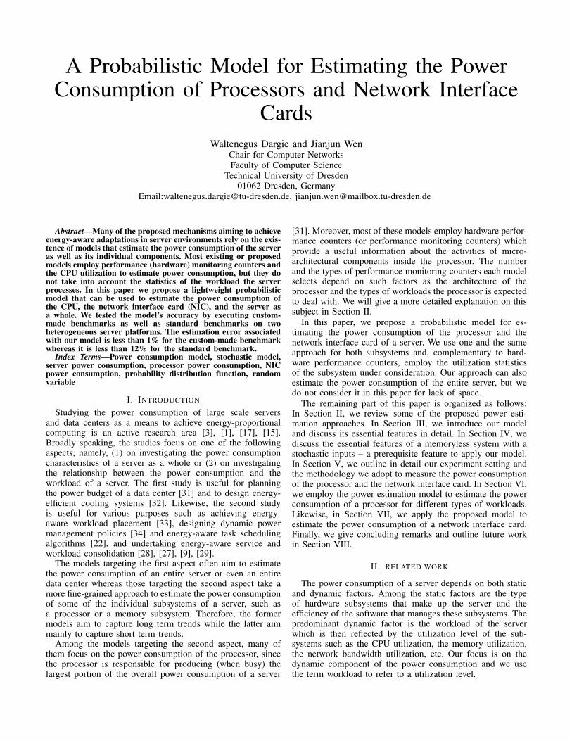
To highlight our point, we shall begin by assuming that therelationship is already known. Hence, we wish to determinethe CDF of one of the random variables (the one whosestatistics we do not know) in terms of the the other (whosestatistics we do know). For example, if the power consumptionof a processor is expressed as:

p = aw + b a, b > 0. (1)

Then, Fp(p) = P{p ≤ p} = P{aw + b ≤ p} =

P{

w ≤[p−ba

]}= Fw

([p−ba

]), where Fw(p) refers to

the distribution of w expressed in terms of p. Likewise,the probability density function of p can be expressed as

1The distribution function Fw(w) of the random variable w is defined asFw(w) = P {w ≤ w}, for −∞ ≤ w ≤ ∞. The distribution function isa non-decreasing, right continuous function, i.e., if w1 and w2 are two realnumbers and w2 > w1, then Fw(w2) ≥ Fw(w1), ∀w2, w1.

2The probability density function of w is the derivation with respect to w

of Fw(w), f(w) =dF (w)dw

.

sumption of a server [10], [25], [18], [6], [5]. A contem-porary CPU provides one or more model-specific reg-isters (MSR) that can be used to count certain micro-architectural events (or performance monitor events).The types of events that should be captured by a PMCis specified by a performance event selector (PES), whichis also a MSR. The amount of countable events has beenincreasing with every generation, family, and model ofprocessors. At present, a processor can provide morethan 200 events. The motivation for using PMC is thataccounting for certain events may offer detailed insightinto the reason why the processor consumes power theway it does [4], [22]. PMC do not require the mod-ification of or intrusion into the hardware structure.Moreover, the events they capture can accurately reflectthe activity levels of the processor. There are, how-ever, some challenges with employing hardware perfor-mance counters: Firstly, one is required to have knowl-edge of the low-level counters in order to be able tomeaningfully correlate hardware events with the powerconsumption. Secondly, the identification of the rele-vant counters is strongly dependent on the nature ofthe benchmark and the server architecture. Thirdly,in most server architectures, one may be able to readnot more than a few counters at the same time. Thisin turn may affect the analysis of the existence of cor-relation between the hardware events and the powerconsumption.We propose a light-weight stochastic model to esti-

mate the probability distribution function of the powerconsumed by a hardware system as long as this systemcan be modelled as a memoryless system with a stochas-tic input. This assumption can be satisfied if the powerconsumption and the utilisation of the hardware sys-tem are sampled at an appropriate granularity (in therange of seconds). The only input our model requiresis the statistics of the utilisation. We will demonstratethe scope and usefulness of our model by estimatingthe power consumption of a processor and a networkinterface card of two different servers.

3. A RANDOM VARIABLEA random variable is a variable whose values are

governed by an underlying probabilistic condition. Inother words, the domain of the random variable is as-sociated with a probability of occurrence. The distri-bution function F (w) of the random variable w1 is afunction that specifies the probability that the value ofw is less than or equal to the real number w. Hence,F (w) = P{w ≤ w}, −∞ ≤ w ≤ ∞. For example,F (30) = 0.7 means the probability that the value ofw being 30 or less is 0.7. F (w) is a non-decreasing,

1We represent a random variable with a boldface small letterwhile the particular instance (value) of the random variableis represented by a plain letter.

p

ww2w1

p2

p1

Figure 1: A one-to-one relationship between pand w results in F (pi) being equal to F (wi).

right continuous function, i.e., if w1 and w2 are two realnumbers and w2 > w1, then F (w2) ≥ F (w1), ∀w2, w1.The probability density function (pdf) of w is the

derivative with respect to w of F (w), i.e., f(w) = dF (w)dw .

The distribution function of w can be obtained by inte-grating the pdf of w: F (w) =

∫ w

−∞ f(τ)dτ . If f(w) = 0

for w < 0, then F (0) = 0 and F (w) =∫ w

0 f(τ)dτ .If two random variables are related with each other,

it is possible to express the distribution and the den-sity function of one of the random variables (whosestochastic properties are not known) in terms of theother (whose stochastic properties may be known). Forexample, if the random variables w and p are relatedas: p = aw + b, a > 0, then, F (p) = P{p ≤ p} =P{aw + b ≤ p} = P{w ≤ p−b

a }, which is the distribu-

tion of w expressed in terms of(

p−ba

). To denote that

the distribution of p can be expressed in terms of thedistribution of w, we use the following notation: Fw(p).If the two random variables have a one-to-one rela-

tionship, then expressing F (p) in terms of F (w) andvice versa becomes interesting. For example, the re-lationship p = aw + b is a one-to-one relationship,since the expression has only one solution ∀w. Likewise,p = aw2 + b has a single solution for w > 0. As can beseen in Figure 1, because of the one-to-one relationshipbetween p and w, P{p ≤ p1} if and only if P{w ≤ w1};likewise, P{p ≤ p2} if and only if P{w ≤ w2}. Fromthis we can conclude that

F (pi) = F (wi), ∀i ∈ R (1)

The significance of this observation becomes clear inSection 4.

4. POWER MODELSuppose we observed in the time interval [t1, t2] the

utilisation pattern (w) and the power consumption (p)of the processor (see Figure 2) and determined that their

3

Fig. 1. Exploiting the one-to-one relationship between p and w andthe monotonic nature of distribution functions to determine a quantitativerelationship between w and p.

ddp (Fp(p)) =

1afw

([p−ba

]), where fw(p) refers to the density

of w expressed in terms of p. If, for instance, the densityof w is exponential: f(w) = λe−λw, λ > 0, where λis the inverse of the mean of the random variable, then,fp(p) =

λa e

−λ([ p−ba ]).

B. Unknown RelationshipIf, however, the relationship between w and p is not known

(which is why we need to develop a model), then the task canbe considered as the inverse process of Section III-A. Hence,given two distribution functions Fw(w) and Fp(p) which weknow are related to each other, our task is to determine theexact nature of the relationship. In other words, we providethe system a workload of known statistics and observe thestatistics of the power consumption of the system. Then weshould find a function g(w) such that the distribution of p =g(w) equals Fp(p).

If the relationship between p and w can be estimated asa one-to-one function, i.e., every element of the range of pcorresponds to exactly one element of the domain of w3,then P {p ≤ pi} equals to P {w ≤ wi} because p ≤ piif and only if w ≤ wi. This can be better visualized inFigure 1 which displays a one-to-one function. From thefigure it is apparent that the value p2 corresponds to w2.Therefore, P {p ≤ p2} corresponds to P {w ≤ w2}. Similarly,P {p ≤ p1} corresponds to P {w ≤ w1}. From this, we canconclude that for a one-to-one function:

Fp(pi) = P {p ≤ pi} = P {w ≤ wi} = Fw(wi) (2)

Subsequently, using Equation 2, we can express p in termsof Fw(p) and Fw(w) as follows:

pi = F−1P (Fw(wi)) (3)

where F−1p refers to the inverse of Fp(p) [35]. For example,

if we observe a uniformly distributed power consumption inthe rage of (10, 50) W for an exponentially distributed work-load, Fw(w) = 1 − e−λw, λ > 0, then, using Equation 2 wehave:

(1− e−λw

)= 1

40p, from which, p = 40(1 − e−λw) =40Fw(w).

3For example, the function p = aw + b is a one-to-one function, since phas exactly one solution ∀w. Likewise, p = aw2 + b has a single solutionfor w > 0.

IV. MEMORYLESS PROPERTY

Equation 3 is a useful expression, but its usefulness is boundto two conditions, namely, (1) the system is memoryless and(2) the workloads should be statistically stationary. Fulfillingthe second condition is possible, since the stochastic propertyof the workload can be controlled during the experiment. Ful-filling the second condition requires choosing the appropriatemeasurement granularity – if the sampling interval is finegrained, the system may not be considered as a memorylesssystem, because there can be a strong dependency betweenthe samples of the measurement. This is particularly trueof processors. If, on the other hand, there is a sufficientdistance between the samples of the power consumption andthe utilization (for the processors we considered, a samplinginterval in the range of hundred milliseconds was sufficient),then the dependency between the samples becomes weak andthe system can be regarded as memoryless.

The autocorrelation function, Rww(t2, t1) = E[w(t2)w(t1)][35], is the best tool to measure the degree of dependencybetween the samples of a stationary random process, w(t). Thedifference between t2 and t1 refers to the time lag between thesamples. For a memoryless system, Rpp(t2, t1) ≈ 0 for t2 6= t1if Rww(t2, t1) ≈ 0 for t2 6= t1. Rpp(t2, t1) and Rww(t2, t1)are the autocorrelation functions of p and w, respectively.

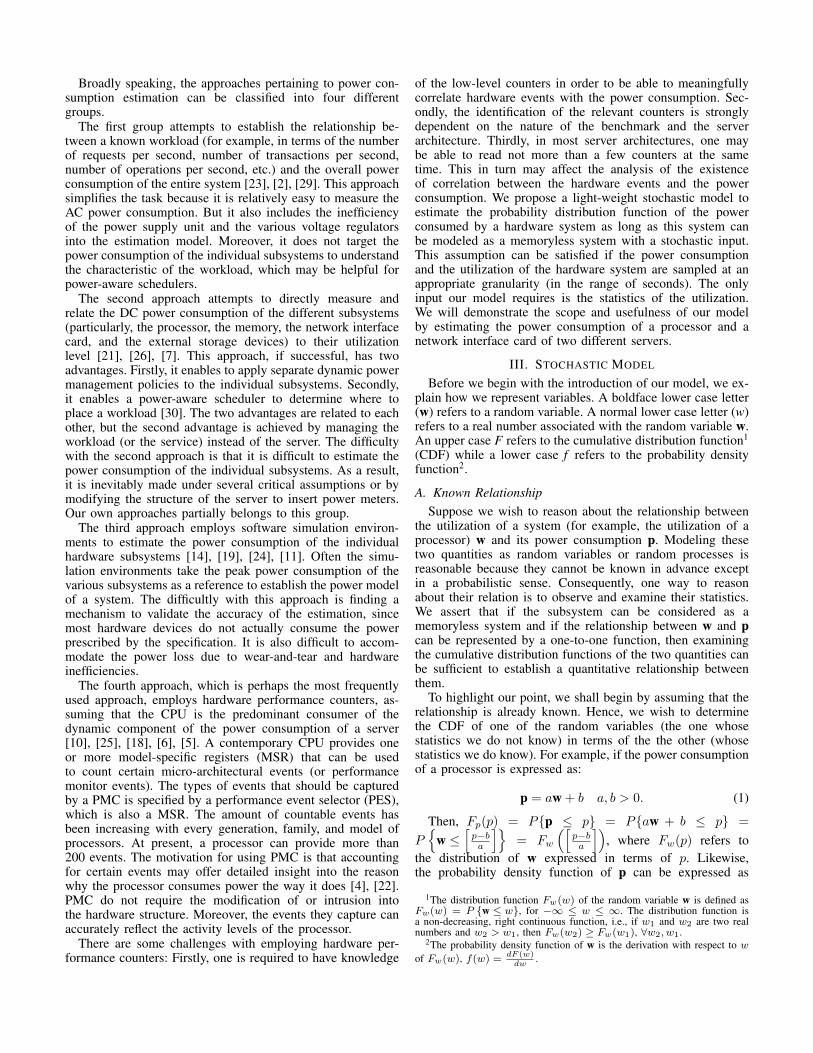
Figure 2 displays the autocorrelation functions of uniformlydistributed CPU and NIC workloads (utilization). For bothdevices the utilization was sampled every second. The auto-correlation of the CPU utilization displays the existence of anapparent correlation for a time lag less than eight seconds,because we deliberately introduced dependency between thesamples of the eight consecutive seconds (we refer the readerto Section 5 to learn how the CPU workload was generated).For a time lag of greater than eight seconds, however, theautocorrelation drops nearly to zero. Likewise, the autocorre-lation of the NIC workload drops sharply for t = t2− t1 > 0.These observation confirm that for a sampling interval of onesecond or even a few hundred milliseconds, our assumptionthat the two systems can be modeled as memoryless systemswith stochastic inputs is plausible.

Figure 3 shows the autocorrelation functions of the corre-sponding power consumptions of the CPU and the NIC. Unlikethe workloads which were sampled every second, we sampledthe power consumption every 250 ms on average becauseof the relatively high resolution of the devices we used tomeasure power (Yokogawa WT210 digital power analyzers).Therefore the time lag 240 in Figure 3 corresponds to the60 s time lag in Figure 2. With this adjustment and takinginto account how we generated the workload of the CPU,it is clear that the correlation between the samples becomesweak for a time lag greater than 32 (corresponding to 8 s),confirming our assumption that the processor can indeed beregarded as a memoryless system. The autocorrelation of thepower consumption of the NIC dropped to zero for t2−t1 > 0,since all the samples of the workload were independent.

V. EXPERIMENT SETTING

In this section, we explain how we applied the conceptswe developed in the previous sections to estimate the powerconsumption of a processor and a network interface card (NIC)based on their utilization statistics.

We performed our experiment on two heterogeneous serverplatforms. The first one was built on a D2581 Siemens-Fujitsu

w

100= 1− e−λp (14)

Therefore,

p = − 1

λln(1− w

100

)(15)

Equation 15 complies with the expression given inEquation 13.

5. MEMORYLESS SYSTEMSEquation 13 is a useful expression, but its usefulness

is bound by two elementary conditions, namely, (1) thesystem is a memoryless system and (2) the workloadsshould be stochastically stationary. Fulfilling the sec-ond condition is feasible, since the stochastic propertyof the workload can be controlled during the experi-ment. Fulfilling the second condition requires choos-ing the appropriate measurement granularity – if thesampling interval is fine grained, the processor may notbe considered memoryless. Fortunately, a service con-solidation process involves a service migration as wellas switching off and/or switching on physical servers.These tasks usually take a few seconds or even a fewhundred seconds. In this regard, it is sufficient to sam-ple the power consumption and the resource utilisationof the server every few milliseconds or every second. Weshall experimentally demonstrate that at this samplinggranularity, we can consider the processor as a memo-ryless system.The autocorrelation function, Rww(τ) = E [w(t)w(t+ τ)],

is the best tool to measure the degree of dependencybetween the samples of the stationary random process,w(t). τ refers to the time lag between the samples. Forthe memoryless system depicted in Figure 2, Rpp(τ) ≈ 0for τ = 0 if Rww(τ) ≈ 0 for τ = 0, where Rpp(τ) andRww(τ) are the autocorrelation functions of p and w,respectively.Figure 3 displays the autocorrelation functions of uni-

formly distributed CPU and NIC workloads. In all thecases, the workloads were sampled every second. Theautocorrelation of the CPU workload displays the ex-istence of an apparent correlation for a time lag lessthan eight seconds, because we deliberately introduceddependency between the samples of the eight consecu-tive seconds (refer to Section 6 to understand how theCPU workload was generated). For a time lag of greaterthan eight seconds, however, the autocorrelation dropsnearly to zero. Likewise, the autocorrelation of the NICworkload drops drastically for t = 0. This observation isimportant due to our assumption that the two systemscan be modelled as memoryless systems with stochasticinputs.Figure 4 shows the autocorrelation function of the

corresponding power consumption of the CPU and the

0 10 20 30 40 50 60

0.0

0.2

0.4

0.6

0.8

1.0

t(s)

Rw

w(t)

: CP

U

0 10 20 30 40 50 60

0.0

0.2

0.4

0.6

0.8

1.0

t(s)

Rw

w(t)

: NIC

:

Figure 3: The autocorrelation function of uni-formly distributed CPU (top) and NIC (bottom)workloads. Maximum time lag = 60 seconds.

NIC. Unlike the workloads which were sampled everysecond, we sampled the power consumption every 250ms on average because of the relatively high resolutionof the device we used – we employed Yokogawa WT210digital power analysers to measure the power consump-tion. Therefore the time lag 240 in Figure 4 correspondsto the 60 s time lag in Figure 3. With this adjustmentand taking into account how we generated the workloadof the CPU, it is clear that the correlation between thesamples becomes weak for a time lag greater than 32(corresponding to 8 s), confirming our assumption thatthe processor can indeed be modelled as a memorylesssystem. The autocorrelation of the power consumptionof the NIC plunged to zero for τ = 0, since all thesamples of the workload were deliberately made inde-pendent.

6. METHODOLOGYIn this section, we will show how we applied the con-

cepts we have developed in the previous section to esti-mate the power consumption of a processor and a net-work interface card (NIC) as a function of the proces-sor and the network bandwidth utilisation (workload)statistics.We carried out our experiment on two heterogeneous

server platforms. The first one was built on a D2581

5

w

100= 1− e−λp (14)

Therefore,

p = − 1

λln(1− w

100

)(15)

Equation 15 complies with the expression given inEquation 13.

5. MEMORYLESS SYSTEMSEquation 13 is a useful expression, but its usefulness

is bound by two elementary conditions, namely, (1) thesystem is a memoryless system and (2) the workloadsshould be stochastically stationary. Fulfilling the sec-ond condition is feasible, since the stochastic propertyof the workload can be controlled during the experi-ment. Fulfilling the second condition requires choos-ing the appropriate measurement granularity – if thesampling interval is fine grained, the processor may notbe considered memoryless. Fortunately, a service con-solidation process involves a service migration as wellas switching off and/or switching on physical servers.These tasks usually take a few seconds or even a fewhundred seconds. In this regard, it is sufficient to sam-ple the power consumption and the resource utilisationof the server every few milliseconds or every second. Weshall experimentally demonstrate that at this samplinggranularity, we can consider the processor as a memo-ryless system.The autocorrelation function, Rww(τ) = E [w(t)w(t+ τ)],

is the best tool to measure the degree of dependencybetween the samples of the stationary random process,w(t). τ refers to the time lag between the samples. Forthe memoryless system depicted in Figure 2, Rpp(τ) ≈ 0for τ = 0 if Rww(τ) ≈ 0 for τ = 0, where Rpp(τ) andRww(τ) are the autocorrelation functions of p and w,respectively.Figure 3 displays the autocorrelation functions of uni-

formly distributed CPU and NIC workloads. In all thecases, the workloads were sampled every second. Theautocorrelation of the CPU workload displays the ex-istence of an apparent correlation for a time lag lessthan eight seconds, because we deliberately introduceddependency between the samples of the eight consecu-tive seconds (refer to Section 6 to understand how theCPU workload was generated). For a time lag of greaterthan eight seconds, however, the autocorrelation dropsnearly to zero. Likewise, the autocorrelation of the NICworkload drops drastically for t = 0. This observation isimportant due to our assumption that the two systemscan be modelled as memoryless systems with stochasticinputs.Figure 4 shows the autocorrelation function of the

corresponding power consumption of the CPU and the

0 10 20 30 40 50 60

0.0

0.2

0.4

0.6

0.8

1.0

t(s)

Rw

w(t)

: CP

U

0 10 20 30 40 50 60

0.0

0.2

0.4

0.6

0.8

1.0

t(s)

Rw

w(t)

: NIC

:

Figure 3: The autocorrelation function of uni-formly distributed CPU (top) and NIC (bottom)workloads. Maximum time lag = 60 seconds.

NIC. Unlike the workloads which were sampled everysecond, we sampled the power consumption every 250ms on average because of the relatively high resolutionof the device we used – we employed Yokogawa WT210digital power analysers to measure the power consump-tion. Therefore the time lag 240 in Figure 4 correspondsto the 60 s time lag in Figure 3. With this adjustmentand taking into account how we generated the workloadof the CPU, it is clear that the correlation between thesamples becomes weak for a time lag greater than 32(corresponding to 8 s), confirming our assumption thatthe processor can indeed be modelled as a memorylesssystem. The autocorrelation of the power consumptionof the NIC plunged to zero for τ = 0, since all thesamples of the workload were deliberately made inde-pendent.

6. METHODOLOGYIn this section, we will show how we applied the con-

cepts we have developed in the previous section to esti-mate the power consumption of a processor and a net-work interface card (NIC) as a function of the proces-sor and the network bandwidth utilisation (workload)statistics.We carried out our experiment on two heterogeneous

server platforms. The first one was built on a D2581

5

Fig. 2. The autocorrelation function of uniformly distributed CPU (top) and NIC (bottom) utilization. Maximum time lag t = (t2 − t1) = 60 seconds.

0 50 100 150 200

0.0

0.2

0.4

0.6

0.8

1.0

t (s/4)

Rpp

(t): C

PU

0 50 100 150 200

0.0

0.2

0.4

0.6

0.8

1.0

t (s/4)

Rpp

(t): N

IC

Figure 4: The autocorrelation function of the power consumption of the CPU (left) and the NIC(right) for uniformly distributed workloads. Maximum time lag = 60 seconds.

Siemens-Fujitsu motherboard integrating a 3.16 GHzIntel E8500 dual core processor and 4 GB DDR2 SDRAMmemory chips. The second server was built on a DB65AlIntel motherboard integrating a 2.5 GHz Intel i5-2400Sdual core processor, 8 GB DDR3 SDRAMmemory chips,and 1GBit Intel network interface card. For testing theprocessor power model we used the E8500 server andfor testing the NIC model, we used the i5-2400S server.The motherboards of both servers provide two DC

power connectors to supply the various subsystems withpower. One of them is a 12 V, 4-pole connector whereasthe other is a 24-pole connector with 12 V, 5 V and 3.3 Vrails (among others). The 12 V rail of the 4-pole connec-tor is exclusively used by the voltage regulators of theprocessor in both motherboards to generate the core-voltages. The voltage regulators draw some amount ofpower from the 5V rail of the 24-pole connector – mainlyused by the Pulse Width Modulator controllers – andit is comparatively very small.The 3.3 V of the 24-pole connector is predominantly

used by the Low Pin Count (LPC) IO controllers. De-vices connected to the PCI and PCI Express cards, suchas the network interface card, exclusively draw powerthrough the 3.3 V rail.For establishing the relationship between the power

consumption and the utilisation of the processor andthe NIC, we generated CPU-bound and IO-bound work-loads having different resource utilisation characteris-tics and run them on the two servers. The CPU-boundworkload was a an infinite loop operation in which in-teger, float point, and shift operation were carried out.While the loop operation executed, it utilised 100% ofthe CPU, but when the loop operation was not exe-cuted, the CPU was idle. In order to generate thedesired workload distribution, we divided time into asequence of one-second none overlapping windows. Wethen generated a set of random numbers in the interval[0, 100] using the runif function of the R statistical toolto make sure that the distribution of the random num-

bers is uniform. In each time window, we picked oneof these random numbers to determine the portion oftime the CPU was fully utilised by the loop operation(between 0 and 100% of the time window). In orderto avoid instability in computation, the proportion ofCPU utilisation for the subsequent eight windows wasmade the same. This means that there was an appar-ent correlation between the eight consecutive windows;otherwise, the random numbers we picked were indepen-dent. The program run for one hour. For testing pur-pose, we executed the loop operation with an exponen-tial distribution and used the SPECPower 2008 bench-mark provided by the Standard Performance Evalua-tion Corporation2. When tested our model while theserver run under three different dynamic frequency andvoltage scaling policies.To establish the relationship between w and p of the

NIC, we followed the same approach, but this time, in-stead of a loop operation, we used an application thatuploads data on the server at different transmissionrates thus varying the amount of network bandwidthutilised per second (MBps) according to a predefinedprobability distribution function, namely, uniform, ex-ponential, and normal distributions. The applicationrun for 15 minutes for each configuration.To measure the power consumption of the NIC, we

connected it with a raiser card which is in turn con-nected to the PCI Express bus. We intercepted the 3.3V rail of the raiser board to directly measure the powerdrawn by the NIC. Figure 5 shows this configuration.

7. PROCESSOR POWER MODELIn this section we will explain how we employed the

expression we obtained in Equations 13 and 1 to es-timate the probability distribution and density func-tions of the power consumption of a processor usingutilisation statistics. In the first step we supplied the

2http://www.spec.org/power ssj2008/.

6

0 50 100 150 200

0.0

0.2

0.4

0.6

0.8

1.0

t (s/4)

Rpp

(t): C

PU

0 50 100 150 200

0.0

0.2

0.4

0.6

0.8

1.0

t (s/4)

Rpp

(t): N

IC

Figure 4: The autocorrelation function of the power consumption of the CPU (left) and the NIC(right) for uniformly distributed workloads. Maximum time lag = 60 seconds.

Siemens-Fujitsu motherboard integrating a 3.16 GHzIntel E8500 dual core processor and 4 GB DDR2 SDRAMmemory chips. The second server was built on a DB65AlIntel motherboard integrating a 2.5 GHz Intel i5-2400Sdual core processor, 8 GB DDR3 SDRAMmemory chips,and 1GBit Intel network interface card. For testing theprocessor power model we used the E8500 server andfor testing the NIC model, we used the i5-2400S server.The motherboards of both servers provide two DC

power connectors to supply the various subsystems withpower. One of them is a 12 V, 4-pole connector whereasthe other is a 24-pole connector with 12 V, 5 V and 3.3 Vrails (among others). The 12 V rail of the 4-pole connec-tor is exclusively used by the voltage regulators of theprocessor in both motherboards to generate the core-voltages. The voltage regulators draw some amount ofpower from the 5V rail of the 24-pole connector – mainlyused by the Pulse Width Modulator controllers – andit is comparatively very small.The 3.3 V of the 24-pole connector is predominantly

used by the Low Pin Count (LPC) IO controllers. De-vices connected to the PCI and PCI Express cards, suchas the network interface card, exclusively draw powerthrough the 3.3 V rail.For establishing the relationship between the power

consumption and the utilisation of the processor andthe NIC, we generated CPU-bound and IO-bound work-loads having different resource utilisation characteris-tics and run them on the two servers. The CPU-boundworkload was a an infinite loop operation in which in-teger, float point, and shift operation were carried out.While the loop operation executed, it utilised 100% ofthe CPU, but when the loop operation was not exe-cuted, the CPU was idle. In order to generate thedesired workload distribution, we divided time into asequence of one-second none overlapping windows. Wethen generated a set of random numbers in the interval[0, 100] using the runif function of the R statistical toolto make sure that the distribution of the random num-

bers is uniform. In each time window, we picked oneof these random numbers to determine the portion oftime the CPU was fully utilised by the loop operation(between 0 and 100% of the time window). In orderto avoid instability in computation, the proportion ofCPU utilisation for the subsequent eight windows wasmade the same. This means that there was an appar-ent correlation between the eight consecutive windows;otherwise, the random numbers we picked were indepen-dent. The program run for one hour. For testing pur-pose, we executed the loop operation with an exponen-tial distribution and used the SPECPower 2008 bench-mark provided by the Standard Performance Evalua-tion Corporation2. When tested our model while theserver run under three different dynamic frequency andvoltage scaling policies.To establish the relationship between w and p of the

NIC, we followed the same approach, but this time, in-stead of a loop operation, we used an application thatuploads data on the server at different transmissionrates thus varying the amount of network bandwidthutilised per second (MBps) according to a predefinedprobability distribution function, namely, uniform, ex-ponential, and normal distributions. The applicationrun for 15 minutes for each configuration.To measure the power consumption of the NIC, we

connected it with a raiser card which is in turn con-nected to the PCI Express bus. We intercepted the 3.3V rail of the raiser board to directly measure the powerdrawn by the NIC. Figure 5 shows this configuration.

7. PROCESSOR POWER MODELIn this section we will explain how we employed the

expression we obtained in Equations 13 and 1 to es-timate the probability distribution and density func-tions of the power consumption of a processor usingutilisation statistics. In the first step we supplied the

2http://www.spec.org/power ssj2008/.

6

Fig. 3. The autocorrelation function of the power consumption of the CPU (left) and the NIC (right) for uniformly distributed workloads. Maximum timelag t = (t2 − t1) = 60 seconds.

motherboard integrating a 3.16 GHz Intel E8500 dual coreprocessor. The second server was built on a DB65Al Intelmotherboard integrating a 2.5 GHz Intel i5-2400S dual coreprocessor and a 1 GBit Intel network interface card. For testingthe processor power model we used the E8500 server and fortesting the NIC model, we used the i5-2400S server.

The motherboards of both servers provide two DC powerconnectors to supply the various subsystems with power. Oneof them is a 12 V, 4-pole connector whereas the other is a 24-pole connector with 12 V, 5 V and 3.3 V rails (among others).The 12 V rail of the 4-pole connector is exclusively used bythe voltage regulators of the processor in both motherboards togenerate the core voltages. The voltage regulators draw someamount of power from the 5V rail of the 24-pole connectormainly used by the Pulse Width Modulator controllers andit is comparatively very small. The 3.3 V of the 24-poleconnector is predominantly used by the Low Pin Count (LPC)IO controllers. Devices connected to the PCI and PCI Expresscards, such as the network interface card, exclusively drawpower through the 3.3 V rail.

For establishing the relationship between the power con-sumption and the utilization of the processor and the NIC,we generated CPU-bound and IO-bound workloads havingdifferent resource utilization characteristics and executed them

on the two servers. The CPU-bound workload was a con-volution operation in which integer, float point, and shiftoperations were performed. While the convolution operationwas executed, it utilised 100% of the CPU, but when the loopoperation was not executed, the CPU was idle. In order togenerate the desired workload distribution, we divided timeinto a sequence of one-second none overlapping windows. Wethen generated a set of random numbers in the interval [0, 100]using the runif function of the R statistical tool to make surethat the distribution of the random numbers is uniform. In eachtime window, we picked out one of these random numbers todetermine the portion of time the CPU was fully utilized bythe convolution operation (between 0 and 100% of the timewindow).

In order to avoid instability in computation, the proportionof the CPU utilization for the subsequent eight windowswas made the same. This means that there was an apparentcorrelation between the eight consecutive windows; otherwise,the random numbers we picked out were independent. Theprogram run for one hour. For testing the model, we generatedan exponentially distributed convolution operation in additionto the SPEC Power 2008 standard benchmark provided by

Fig. 4. Using a raiser board to intercept the power rails of the PCI Expressto measure the power consumption of the NIC.

the Standard Performance Evaluation Corporation4. We testedour model while the server run under three different dynamicfrequency and voltage scaling policies.

To establish the relationship between w and p of the NIC,we followed the same approach, but this time, instead of theconvolution operation, we used an application that uploadsdata on the i5-2400S server at different transmission rates thusvarying the amount of network bandwidth utilized per second(MBps) according to a predefined probability distributionfunction, namely, uniform and exponential distributions. Theapplication run for 15 minutes for each configuration. Tomeasure the power consumption of the NIC, we connectedit with a raiser card which is in turn connected to the PCIExpress bus. We intercepted the 3.3 V rail of the raiser boardto directly measure the power drawn by the NIC. Figure 4displays the NIC instrumentation.

VI. PROCESSOR POWER CONSUMPTION MODEL

To determine the relationship between the utilization statis-tics of the E8500 Intel processor and its power consumption,we first disabled one of the cores5. Then, we generated a onehour uniformly distributed workload in the interval (0,100) bythe convolution operation. We choose a uniformly distributedworkload because it simplifies the evaluation of Equation 3.During the execution of the convolution operation, we mea-sured the power consumption of the processor and plotted itsFp(p). Then, using R’s nls curve fitting toolbox, we approx-imated Fp(p) which can be best approximated by a quadraticfunction, Fp(p) = a1p

2 + a2p+ a3, 9.45 ≤ p ≤ 32.15, wherea1 = −0.001026, a2 = 0.07765, and a3 = −0.6136 arethe coefficients of the quadratic function. Figure 5 displaysthe experimental and the approximated Fp(p). Hence, for thequadratic functions, we have:

Fp(p) = a1p2 + a2p+ a3 9.54 ≤ p ≤ 32.15 (4)

Fw(w) =w

100, 0 ≤ w ≤ 100 (5)

4www.spec.org/power ssj2008/5The relationship between the workload and the power consumption of

the dual-core processor is linear: p = K4w + K5 where K4 = 3.5 andK5 = 10.5, 0 ≤ w ≤ 100. The derivation of this relationship is beyond thescope of this paper.

Figure 5: Intercepting the 3.3 V rail of the raisercard to measure the power consumption of theNIC.

processor a uniformly distributed workload to establishthe relationship between w and p and then, we usingcustom made and standard benchmarks, we tested theestimation capacity of the relationship.

7.1 Model ParametersFigure 6 displays the distribution function of the ac-

tual power consumption of the E8500 processor in asingle-core setting3 when the processor’s utilisation wasuniformly distributed, i.e., w: U(0, 100%). We approx-imated the distribution with a quadratic function usingMatlab’s curve fitting tool (with coefficient of determi-nation, R2 = 0.957 and a root mean square deviation(RMSD) of 0.0523) as shown by the dashed coral linein the same figure. The estimated quadratic functionFest(p) as a function of the real power consumption ofthe processor is expressed as:

Fest(p) = p1p2 + p2p+ p3, 9.45 ≤ p ≤ 32.15 (16)

where p1 = −0.001026, p2 = 0.07765, p3 = −0.6136and p is the power consumption of the processor definedas a random variable.The distribution of w in the interval [0, 100] is ex-

pressed as: F (w) = w100 . Hence, we have both Fest(p)

and F (w) to make use of Equation 13 and to express pin terms of w:

p =−p2 +

√p22 − 4p1 × (p3 − (w− a) / (b− a))

2× p1(17)

Equation 17 can be expressed as:

p = K1 + (K2w+K3)12 (18)

3The relationship between the workload and the power con-sumption of a dual-core processor is best approximated by alinear relationship. For the E8500 processor: p = K4w+K5

where K4 = 3.5 and K5 = 10.5, 0 ≤ w ≤ 100. The deriva-tion of this relationship is beyond the scope of this paper.

10 15 20 25 30 35

0.0

0.2

0.4

0.6

0.8

1.0

p (W)

Fp(p

)

ActualEstimated

Figure 6: The actual (dark solid line) and ap-proximated (dashed coral) CDF of the powerconsumption of the CPU for a uniformly dis-tributed utilisation.

where K1 = − p2

2p1, K2 = 1

p1(b−a) , and K3 =p22

4p12 −

ap1(b−a) −

p3

p1.

Equation 18 is the desired relationship we wished toestablish between the CPU utilisation and the CPUpower consumption. Using this relationship, it is nowpossible to determine the distribution and density of pin terms of the distribution and density of w for anyarbitrary w.Earlier, we showed that F (p) can be expressed as

P{p ≤ p} = P{g(w) ≤ p}. Hence,

F (p) = P{(

K1 + (K2w+K3)12

)≤ p}, 0 ≤ w ≤ 100

(19)Expressing Equation 19 in terms of F (w) yields:

Fw(p) = P

{w ≤ (p−K1)

2 −K3

K2

}, 0 ≤ w ≤ 100

(20)

which is the same as Fw

((p−K1)

2−K3

K2

). Likewise, the

density of p can be expressed as:

f(p) =

∣∣∣∣2

K2(p−K1)

∣∣∣∣ fw((p−K1)

2 −K3

K2

)(21)

7.2 Model ValidationTo validate the relationship we established in Equa-

tions 17 and 18, we used both a custom made anda standard benchmark. The custom made benchmarkwas the one we used to establish the model parameters,but this time it had an exponential distribution insteadof a uniform distribution. Moreover, the exponentialdistribution workload had different means (μ = 5 andμ = 15) as well as execution durations (10, 20, and 30minutes). The standard benchmark is the SPECPower2008 benchmark, specially developed to test the power

7

Fig. 5. The actual (measured) and estimated values of Fp(p) of the uniformlydistributed utilization U(10, 90) for the Intel E8500 dual core processor.

By inserting Equation 4 and 5 into Equation 3, we obtain:

p =−a2 +

√a22 − 4a1 ×

(a3 − w

100

)2× a1

(6)

Equation 6 can be expressed as:

p = K1 + (K2w +K3)12 (7)

where K1 = − a22a1

, K2 = 1a1(100)

, and

K3 =a224a1− b

a1(100)− a3

a1.

Equation 7 is the desired relationship we wished to establishbetween the CPU workload and the power consumption.Using this relationship, it is now possible to estimate theruntime power consumption of the processor as long as wecan predict its utilization. Moreover, using Equation 7, wecan determine the distribution and density of p for a workloadof arbitrary distribution and density.

Earlier, we showed that Fp(p) can be expressed as P{p ≤p} = P{g(w) ≤ p}. Hence,

Fp(p) = P{(K1 + (K2w +K3)

12

)≤ p}

0 ≤ w ≤ 100

(8)Expressing Equation 8 in terms of Fw(w) yields:

Fw(p) = P

{w ≤ (p−K1)

2 −K3

K2

}b ≤ w ≤ c (9)

which is the same as Fw

((p−K1)

2−K3

K2

). Likewise, the

density of p can be expressed as:

fp(p) =

∣∣∣∣2

K2(p−K1)

∣∣∣∣ fw((p−K1)

2 −K3

K2

)(10)

A. Theoretical Fp(p) and fp(p)Using the relationship expressed in Equation 7, it is possible

to compute the distribution and density functions of p for aworkload of arbitrary probability density function. We shalldemonstrate this by computing the theoretical density anddistribution functions of p for an exponentially distributedworkload. In the subsection that will follow we shall compare

10 15 20 25 300

0.2

0.4

0.6

0.8

1

p(W)

Fp

(p)

A:E(5),d=10mA:E(5),d=20mA:E(5),d=30mE:E(5)A:E(15),d=10mA:E(15),d=20mA:E(15),d=30mE:E(15)

Figure 7: The probability distribution functionof the power consumed by the processor when its10, 20, and 30 minute utilisation was exponen-tially distributed. The solid lines indicate theactual power consumption whereas the dashedlines indicate the estimated distribution usingthe inverse relation in Equation 13.“A” refers tothe actual power consumption and “E” to theestimated.

consumption of Internet based servers. To test thestrength of our model, we run the server under differentdynamic frequency and voltage scaling policies whileexecuting the SPECPower 2008 benchmark – namely,performance, conservative, and on-demand policies. Forthe detail of these policies, we refer our reader to ourprevious work [13, 8].Figure 7 displays the distribution function of the ac-

tual and estimated power consumption of the processorfor the exponentially distributed utilisation. All solidlines indicate actual power consumptions while the twodashed lines are the estimated distributions for μ = 5and μ = 15. Understandably, there is a little deviationin the estimated power consumptions of the processorfor the different execution durations. It is to be notedthat we generated random numbers to determine theportion of a time slot the CPU should be 100% busy.Each time we generated these numbers we got differentresults. Moreover, the number of samples we obtainedfor the different execution durations (10, 20, and 30minutes) was different. This resulted in a reasonablysmall deviation in the power consumptions estimated.Otherwise, Equation 17 was able to estimate the distri-bution of the power consumption with an average stan-dard error of 0.009559.Figure 8 displays the probability density functions of

the actual and estimated power consumed by the E8500processor when executing the SPECPower 2008 bench-mark. Unlike the exponentially distributed workload,the SPECPower benchmark occupies the entire utilisa-tion spectrum which in turn resulted is a wider powerconsumption spectrum, which is difficult to estimate.Moreover, we obtained the model parameters of Equa-tion 18 when the server was running under the per-formance policy in which the processor frequency was

set to the maximum during the entire operation. How-ever, when we tested the model, the processor operationvoltages and frequencies were varied based on the an-ticipated workload. Even so, our model was able toestimate the power consumption of the processor in allpower management settings. The combined average es-timation error was 7.3%. The error is a small amoutcompared to the simplicity of our model, which usesa single input, unlike most existing or proposed powerestimation models (see Related Work), which have mul-tiple parameters that are difficult to obtain or may nottransfer well from one processor architecture to another.

8. NIC POWER MODELSimilar to Section 7, we will employ Equations 13

and 1 to estimate the probability distribution and den-sity functions of the power consumption of a networkinterface card. Hence, we will first show how the rela-tionship betweenw an p was determined for a uniformlydistribution bandwidth utilisation and then, how, usingthe relationship, we estimated the power consumptionstatistic of the NIC for a utilisation of arbitrary statis-tics.

8.1 Model ParametersFigure 9 – the solid black line – shows the power

consumption of the network interface card when its 15minute bandwidth utilisation was uniformly distributedbetween 0 and 125 MBps. We approximated this distri-bution using curve fitting by the following expression:

Fest(p) = 1− 6e−p2

(22)

Since the network bandwidth utilisation varied uni-formly, we have F (w) = w

125 for 0 ≤ w ≤ 125 MBps.Thus using the inverse relation we obtained in Equa-tion 13, the power consumption of the network interfacecard can be expressed as follows:

p =

√−ln

[125−w

750

](23)

And the probability distribution function of p in termsof the distribution function of w is expressed as:

F (p) = Fw

(1− 6e−p2

)(24)

And the density of p is expressed as:

f(p) = 12pe−p2

fw

([125− 600e−p2

])(25)

8.2 Model ValidationFigure 9 (bottom) displays the power consumption

of the NIC when its bandwidth utilisation was expo-nentially distributed. We have considered three cases:

8

Fig. 6. The actual (A) and estimated (E) F (p) of the Intel E8500 processorwhen executing exponentially distributed workloads.

the theoretical result with the one we obtained from anexperiment.

1) Exponentially distributed workload: When w is expo-nentially distributed (f(w) = λe−λw;µ = 1

λ ), its distributionfunction equals:

Fp(w) = 1− e−wµ b ≤ w ≤ c (11)

And the probability density function of p can be expressedas follows:

fp(p) =

∣∣∣∣2

K2(p−K1)

∣∣∣∣ e−(((p−K1)

2−K3)/K2)/µ (12)

The distribution function of p is expressed as:

Fp(p) = Fw(p) = 1− e−(((p−K1)2−K3)/K2)/µ (13)

where p is in the interval [9.45, 32.15] and Fw(p) refers tothe probability distribution function of w expressed in termsof p.

B. Experimental F (p)After having established the relationship between p and w,

we tested the validity of our model by generating custom-madeexponentially distributed workloads and the SPEC Powerbenchmark. The workloads with the exponential distributionhad the following average utilization: µ = 5%, 10%, 15%and 20%. To ensure that our model was time invariant, wegenerated the workloads for the duration of 10, 20, and 30minutes (i.e., the sample size of the workload for each test casewas different). Figure 6 displays the theoretically estimated(the dashed lines) and the experimentally obtained (solid lines)Fp(p) for the exponentially distributed workloads of the E8500processor. As can be seen from the figure, when the testworkload was similar in type with the training workload (inboth cases we used the convolution operation), its powerconsumption could be accurately predicted (with an averageerror < 1%) even though the statistics of the workloads weredissimilar and the durations of the workloads were differentfor the test cases.

Similarly, we tested our model with theSPECpower ssj2008 (SPEC Power) benchmark. TheSPEC Power “is the first industry-standard SPEC benchmarkthat evaluates the power and performance characteristics of

20 40 60 80

0.00

00.

005

0.01

00.

015

w(%)

f(w

)

Fig. 7. The actual workload distribution of the SPEC power benchmark.

volume server class and multi-node class computers”6. Thefull SPEC power benchmark runs for 70 minutes. We testedthe model while the server operated under different dynamicvoltage and frequency scaling policies, to examine how itsestimation accuracy was affected by frequency and voltagevariations (real-world servers often employ dynamic voltageand frequency scaling for energy-efficient operation). Thepolicies we examined were the performance, conservative,and on-demand policies. For the detail of these policies, werefer our reader to our previous work [13, 8]. The conservativeand on-demand policies vary the frequency and core voltageof the processor depending on its anticipated future workloadusing exponential moving average filters to predict the futureworkload of the processor. Figure 8 displays the probabilitydensity functions of the actual and estimated power consumedby the E8500 processor when executing the SPEC Powerbenchmark. Unlike the exponentially distributed workload,the SPEC Power benchmark occupies the entire utilizationdomain (see Figure 7) which in turn resulted in a widerpower consumption range.

It must be noted that the model parameters of Equation 7were obtained when the server was operating at maximum corevoltage and maximum operation frequency whereas when wetested the model, the processor operation voltages and fre-quencies were dynamically varied by the power managementpolicies. Even so, our model was able to estimate the powerconsumption of the processor in all the power managementsettings with comparable accuracy. The average estimationerror was 11.3%.

VII. NIC POWER MODEL

Similar to Section VI, we employed Equations 2 and 3 toestimate the power consumption of the network interface cardof the i5-2400S server. We shall show how the relationshipbetween w and p was determined for a uniformly distributedbandwidth utilization and how, using the relationship, weestimated the power consumption statistic of the NIC for autilization of arbitrary statistics.

6http://www.spec.org/power ssj2008/

5 10 15 20 25 30 35

0.00

0.02

0.04

0.06

0.08

0.10

p(W)

fp(p

)

ActualEstimated

5 10 15 20 25 30 35

0.00

0.02

0.04

0.06

0.08

0.10

p(W)

fp(p

)

ActualEstimated

5 10 15 20 25 30 35

0.00

0.02

0.04

0.06

0.08

0.10

p(W)

fp(p

)

ActualEstimated

Figure 8: The probability density function of the actual and estimated power consumption of theprocessor for the SPECPower benchmark. The processor was running under the performance (left),conservative (middle), and on-demand (right) dynamic voltage and frequency scaling policies.

1.3 1.4 1.5 1.6 1.7 1.8 1.9

0.0

0.2

0.4

0.6

0.8

1.0

p (W)

Fp(p

)

●●●●●●●●●●●●●●●●●●●●●●●●●●●●●●●●●●●●●●●●●●●●●●●●●●●●●●●●●●●●●●●●●●●●●●●●●●●●●●●●●●●●●●●●●●●●●●●●●●●●●●●●●●●●●●●●●●●●●●●●●●●●●●●●●●●●●●●●●●●●●●●●●●●●●●●●●●●●●●●●●●●●●●●●●●●●●●●●●●●●●●●●●●●●●●●●●●●●●●●●●●●●●●●●●●●●●●●●●●●●●●●●●●●●●●●●●●●●●

●●●●●●●●●●●●●●●●●●●●●●●●●●●●●●●●●●●●●●

●●●●●●●●●●●●●●●●●●●●●●●●●●●●●●●●●●●●●●●●●●●●●●●●●

●●●●●●●●●●●●●●●●●●●●●●●●●●●●●●●●●●●●●●●●●●●●●●●●●●●●●●●●●●●●

●●●●●●●●●●●●●●●●●●●●●●●●●●●●●●●●●●●●●●●●●●●●●●●●●●●●●●●●●●●●●●●

●●●●●●●●●●●●●●●●●●●●●●●●●●●●●●●●●●●●●●●●●●●●●●●●●●

●●●●●●●●●

ActualEstimated

E: E(10)A: E(10)E: E(20)A: E(20)A: E(50)E: E(50)

Figure 9: Top: The probability distributionfunction of the actual and estimated powerconsumption of the NIC during the trainingphase ( 15 minutes uniformly distributed band-width utilisation). Bottom: The distributionof the power consumption of the NIC duringthe testing phase (for 15 minutes exponentiallydistributed bandwidth utilisation of differentmeans) – “A” stands for Actual and “E” for Es-timated.

μ = 10, 20, 50. Except for the case μ = 50, the relation-ship in Equation 24 was able to accurately estimate thepower consumption of the NIC based on knowledge ofthe stochastic of the bandwidth utilisation (with a stan-dard error that equals 0.00955). The estimation errorwas larger for μ = 50 (a standard error of 0.0146). Thejustification for this is similar to the one we gave to theSPECPower benchmark. As the utilisation spectrumincreases, the accumulated estimation error increases aswell. Even so, the estimation error can be considerednegligible.

9. CONCLUSIONWe proposed a stochastic model to estimate the power

consumption of the different subsystems of a server in adata centre. Our model uses two variables only, namely,the stochastic of the utilisation level (w) and the ac-tual power consumption (p), both obtainable in anyserver platform. In this model the probability distri-bution function played a vital role in establishing therelationship between w and p.We demonstrated the scope and usefulness of our ap-

proach by estimating the power consumption of the pro-cessor and the network interface card of two heteroge-neous servers for a variety of workload statistics. Alto-gether we ran 16 test cases and observed that the modelwas indeed accurate.This said, the model is useful for memoryless sys-

tems, which means, the sampling interval should be bigenough to ensure that the samples of the power con-sumption can be considered statistically independent.But in a typical service consolidation scenario this is ac-tually the case. Our model performed relatively poorlyfor the SPECPower benchmark. This is because, the es-timation region occupies the entire utilisation spectrumof the processor thereby accumulating the estimationerror. A typical Internet server may not have such a

9

Fig. 8. The probability density function of the actual and estimated power consumption of the processor for the SPEC Power benchmark. The processorwas running under the performance (left), conservative (middle), and on-demand (right) dynamic voltage and frequency scaling policies.

5 10 15 20 25 30 35

0.00

0.02

0.04

0.06

0.08

0.10

p(W)

fp(p

)

ActualEstimated

5 10 15 20 25 30 35

0.00

0.02

0.04

0.06

0.08

0.10

p(W)

fp(p

)

ActualEstimated

5 10 15 20 25 30 35

0.00

0.02

0.04

0.06

0.08

0.10

p(W)

fp(p

)

ActualEstimated

Figure 8: The probability density function of the actual and estimated power consumption of theprocessor for the SPECPower benchmark. The processor was running under the performance (left),conservative (middle), and on-demand (right) dynamic voltage and frequency scaling policies.

1.3 1.4 1.5 1.6 1.7 1.8 1.9

0.0

0.2

0.4

0.6

0.8

1.0

p (W)

Fp(p

)

●●●●●●●●●●●●●●●●●●●●●●●●●●●●●●●●●●●●●●●●●●●●●●●●●●●●●●●●●●●●●●●●●●●●●●●●●●●●●●●●●●●●●●●●●●●●●●●●●●●●●●●●●●●●●●●●●●●●●●●●●●●●●●●●●●●●●●●●●●●●●●●●●●●●●●●●●●●●●●●●●●●●●●●●●●●●●●●●●●●●●●●●●●●●●●●●●●●●●●●●●●●●●●●●●●●●●●●●●●●●●●●●●●●●●●●●●●●●●

●●●●●●●●●●●●●●●●●●●●●●●●●●●●●●●●●●●●●●

●●●●●●●●●●●●●●●●●●●●●●●●●●●●●●●●●●●●●●●●●●●●●●●●●

●●●●●●●●●●●●●●●●●●●●●●●●●●●●●●●●●●●●●●●●●●●●●●●●●●●●●●●●●●●●

●●●●●●●●●●●●●●●●●●●●●●●●●●●●●●●●●●●●●●●●●●●●●●●●●●●●●●●●●●●●●●●

●●●●●●●●●●●●●●●●●●●●●●●●●●●●●●●●●●●●●●●●●●●●●●●●●●

●●●●●●●●●

ActualEstimated

E: E(10)A: E(10)E: E(20)A: E(20)A: E(50)E: E(50)

Figure 9: Top: The probability distributionfunction of the actual and estimated powerconsumption of the NIC during the trainingphase ( 15 minutes uniformly distributed band-width utilisation). Bottom: The distributionof the power consumption of the NIC duringthe testing phase (for 15 minutes exponentiallydistributed bandwidth utilisation of differentmeans) – “A” stands for Actual and “E” for Es-timated.

μ = 10, 20, 50. Except for the case μ = 50, the relation-ship in Equation 24 was able to accurately estimate thepower consumption of the NIC based on knowledge ofthe stochastic of the bandwidth utilisation (with a stan-dard error that equals 0.00955). The estimation errorwas larger for μ = 50 (a standard error of 0.0146). Thejustification for this is similar to the one we gave to theSPECPower benchmark. As the utilisation spectrumincreases, the accumulated estimation error increases aswell. Even so, the estimation error can be considerednegligible.

9. CONCLUSIONWe proposed a stochastic model to estimate the power

consumption of the different subsystems of a server in adata centre. Our model uses two variables only, namely,the stochastic of the utilisation level (w) and the ac-tual power consumption (p), both obtainable in anyserver platform. In this model the probability distri-bution function played a vital role in establishing therelationship between w and p.We demonstrated the scope and usefulness of our ap-

proach by estimating the power consumption of the pro-cessor and the network interface card of two heteroge-neous servers for a variety of workload statistics. Alto-gether we ran 16 test cases and observed that the modelwas indeed accurate.This said, the model is useful for memoryless sys-

tems, which means, the sampling interval should be bigenough to ensure that the samples of the power con-sumption can be considered statistically independent.But in a typical service consolidation scenario this is ac-tually the case. Our model performed relatively poorlyfor the SPECPower benchmark. This is because, the es-timation region occupies the entire utilisation spectrumof the processor thereby accumulating the estimationerror. A typical Internet server may not have such a

9

Fig. 9. The actual (measured) and estimated values of Fp(p) of the uniformlydistributed bandwidth utilization for the i5-2400S server.

A. Model Parameters

Figure 9 (the black solid line) displays the distribution ofthe actual power consumption of the NIC when its 15 minutebandwidth utilization was uniformly distributed in the interval[0, 125] MBps. We approximated this distribution using acurve fitting by the following expression (the coral solid linein Figure 9):

Fp(p) = 1− 6e−p2

(14)

Since the network bandwidth utilization varied uniformly,we have Fw(w) = w

125 for 0 ≤ w ≤ 125 MBps. Thus usingthe inverse relation we obtained in Equation 3, the powerconsumption of the network interface card can be expressedas follows:

p =

√−ln

[125− w750

](15)

And the probability distribution function of p in terms ofthe distribution function of w is expressed as:

Fp(p) = Fw

(1− 6e−p

2)

(16)

Finally, the density of p is expressed as:

1.3 1.4 1.5 1.6 1.7 1.8 1.90.

00.

20.

40.

60.

81.

0

p (W)

Fp(

p)●●●●●●●●●●●●●●●●●●●●

●●●●●●●●●●●●●●●●●●●●●●●●●●●●●●●●●●●●●●●●●●●●●●●●●●●●●●●●●●●●●●●●●●●●●●●●●●●●●●●●●●●●●●●●●●●●●●●●●●●●●●●●●●●●●●●●●●●●●●●●●●●●●●●●●●●●●●●●●●●●●●●●●●●●●●●●●●●●●●●●●●●●●●●●●●●●●●

●●●●●●●●●●●●●●●●●●●●●●●●●●●●●●

●●●●●●●●●●●●●●●●●●●●●●●●●●●●●●●●●●●●●●

●●●●●●●●●●●●●●●●●●●●●●●●●●●●●●●●●●●●●●

●●●●●●●●●●●●●●●●●●●●●●●●●●●●●●●●●●●●●●●●●●●●●●●●

●●●●●●●●●●●●●●●●●●●●●●●●●●●●●●●●●●●●●●●●●●●●●●●●●●●●●●●●●●●●

●●●●●●●●●●●●●●●●●●●●●●●●●●●●●●●●●●●●●●●●●●●●●●●●●●●●●●●●●●●●●●●●●●●●●

●●●●●●●●●●●●●●

●●●●●●●●●●●●●●●●●●

●●●●●●●●●●●●●●●●●●●●●●●●●●●●●●●●●●●●●●●●●●●●●●●●●●●●●●●●●●●●●●●●●●●●●●●●●●●●●●●●●●●●●●●●●●●●●●●●●●●●●●●●●●●●●●●●●●●●●●●●●●●●●●●●●●●●●●●●●●●●●●●●●●●●●●

●●●●●●●●●●●●●●●●●●●●●●●●●●●●●●●●●

●●●●●●●●●●●●●●●●●●●●●●●●●●●●●●●●●●●●●●●●●●●●●●●●●●●●●●●●

●●●●●●●●●●●●●●●●●●●●●●●●●●●●●●●●●●●●●●●●●●●●●●●●●●●●●●●●●●●●●●●●●●●●●●●●●●●●●●●●●●●●●

●●●●●●●●●●●●●●●●●●●●●●●●●●●●●●●●●●●●●●●●●●●●●●●●●●●●●●●●●●●●●●●●●●●●●●●●●●●●●●●●●●●●●●●●●●●●●●

●●●●●●●●●●●●●●●●●●●

●●●●●●●●●●●●●●●●●●●●●●●●●●●●●●●●●●●●●●●●●●●●●●●●●●●●●●●●●●●●●●●●●●●●●●●●●●●●●●●●●●●●●●●●●●●●●●●●●●●●●●●●●●●●●●●●●●

●●●●●●●●●●●●●●●●●●●●●●●●●●●●●●●●●●●●●●●●●●●●●●●●●●●●●●

●●●●●●●●●●●●●●●●●●●●●●●●●●●●●●●●●●●●●●●● ●●●●●●●●●● ●● ●● ●●●●●●●

E: 10A: 10E: 20A: 20A: 50E:50

Fig. 10. The actual (measured) and estimated values of Fp(p) of theexponentially distributed bandwidth utilization for the i5-2400S server.

f(p) = 12pe−p2

fw

(125− 600e−p

2)

(17)

B. Model Validation

Figure 10 displays the power consumption of the NIC whenits bandwidth utilization was exponentially distributed. Wehave considered three cases: µ = 10, 20, 50. Except for thecase µ = 50, the relationship in Equation 15 was able toaccurately estimate the power consumption of the NIC basedon knowledge of the statistics of the bandwidth utilization(with a standard error that equals 0.00955). The estimationerror was larger for µ = 50 (a standard error of 0.0146).The justification for this is similar to the one we gave to theSPEC Power benchmark – as the span of the utilization domainincreased, the accumulated estimation error increased as well.Even so, the average estimation error, similar to the estimationerror of the processor for the exponential workload, was < 1%.

VIII. CONCLUSION

We proposed a probabilistic model to estimate the powerconsumption of the different subsystems of a server. Ourmodel uses two variables only, namely, the system’s utilizationstatistics (w) and the statistics of the actual power consumption(p), both are easily obtainable in many server platforms. In ourmodel the cumulative distribution function played a vital role.

We demonstrated the scope and usefulness of our approachby estimating the power consumption of the processor andthe network interface card of two heterogeneous servers for avariety of workload statistics. Altogether we executed 16 testcases. This said, the model is useful for memoryless systems,which means, the sampling interval should be long enoughto ensure that the samples of the workload and the powerconsumption should be statistically independent.

Our model performed relatively poorly for the SPECPowerbenchmark. This is because, the estimation region occupies theentire utilization domain of the processor thereby increasingthe accumulated estimation error. A typical Internet server maynot have such a wide utilization domain. One of the problemswe faced during the testing of our model was the difficulty ofusing curve fitting. Without this step, it was not possible toestablish a relationship between w and p. For a curve fitting toproduce an accurate approximation, the expressions should becomplex. Simple expressions come up with large errors. Butobtaining the inverse of complex expressions is difficult.

In this paper we have not included the memory subsystem,without which it is difficult to estimate the overall DC powerconsumption of a server. Our aim in future is to include it andto compute the contribution of individual components to theoverall power consumption of a server.

REFERENCES

[1] D. Abts, M. R. Marty, P. M. Wells, P. Klausler, and H. Liu. Energyproportional datacenter networks. SIGARCH Comput. Archit. News,38(3):338347, June 2010.

[2] F. Ahmad and T. N. Vijaykumar. Joint optimization of idle and coolingpower in data centers while maintaining response time. In Proceedings ofthe fifteenth edition of ASPLOS on Architectural support for program-ming languages and operating systems, ASPLOS 10, pages 243256, NewYork, NY, USA, 2010. ACM.

[3] L. A. Barroso and U. Holzle. The case for energy-proportional comput-ing. Computer, 40(12):3337, Dec. 2007.

[4] F. Bellosa. The benefits of event. In Proceedings of the 9th workshopon ACM SIGOPS European workshop beyond the PC: new challengesfor the operating system - EW 9, page 37, New York, New York, USA,2000. ACM Press.

[5] R. Bertran, M. Gonzalez, X. Martorell, N. Navarro, and E. Ayguade.Decomposable and responsive power models for multicore processorsusing performance counters. In Proceedings of the 24th ACM Interna-tional Conference on Supercomputing - ICS 10, page 147, New York,New York, USA, 2010. ACM Press.

[6] W. L. Bircher and L. K. John. Complete System Power EstimationUsing Processor Performance Events. IEEE Transactions on Computers,61(4):563577, Apr. 2012.

[7] P. Bohrer, E. N. Elnozahy, T. Keller, M. Kistler, C. Lefurgy, C.McDowell, and R. Rajamony. The case for power management in webservers, pages 261289. Kluwer Academic Publishers, Norwell, MA,USA, 2002.

[8] A. Brihi and W. Dargie. Dynamic voltage and frequency scaling in multi-media servers. In The 27th IEEE International Conference on AdvancedInformation Networking and Applications (AINA-2013), 2013.

[9] G. Chen,W. He, J. Liu, S. Nath, L. Rigas, L. Xiao, and F. Zhao. Energy-aware server provisioning and load dispatching for connection-intensiveinternet services. In Proceedings of the 5th USENIX Symposium on Net-worked Systems Design and Implementation, NSDI08, pages 337350,Berkeley, CA, USA, 2008. USENIX Association.

[10] X. Chen, C. Xu, R. P. Dick, and Z. M. Mao. Performance andpower modeling in a multi-programmed multi-core environment. InProceedings of the 47th Design Automation Conference, DAC 10, pages813818, New York, NY, USA, 2010. ACM.

[11] Y. Chen, A. Das, W. Qin, A. Sivasubramaniam, Q. Wang, and N.Gautam. Managing server energy and operational costs in hostingcenters. SIGMETRICS Perform. Eval. Rev., 33:303314, June 2005.

[12] C. Clark, K. Fraser, S. Hand, J. G. Hansen, E. Jul, C. Limpach, I. Pratt,and A. Warfield. Live migration of virtual machines. In Proceedingsof the 2nd conference on Symposium on Networked Systems Design& Implementation - Volume 2, NSDI05, pages 273286, Berkeley, CA,USA, 2005. USENIX Association.

[13] W. Dargie. Analysis of the power consumption of a multimedia serverunder different DVFS policies. In IEEE CLOUD, 2012.

[14] D. Economou, S. Rivoire, and C. Kozyrakis. Full-system power analysisand modeling for server environments. In The 2nd Workshop onModeling, Benchmarking, and Simulation (MoBS), pages 7077, 2006.

[15] E. N. Elnozahy, M. Kistler, and R. Rajamony. Energy-efficient serverclusters. In Proceedings of the 2nd international conference on Power-aware computer systems, PACS02, pages 179197, Berlin, Heidelberg,2003. Springer-Verlag.

[16] D. Gmach, J. Rolia, L. Cherkasova, and A. Kemper. Resource poolmanagement: Reactive versus proactive or lets be friends. Comput.Netw., 53:29052922, December 2009.

[17] S. Huang and W. Feng. Energy-efficient cluster computing via accurateworkload characterization. In Proceedings of the 2009 9th IEEE/ACMInternational Symposium on Cluster Computing and the Grid, CCGRID09, pages 6875, Washington, DC, USA, 2009. IEEE Computer Society.

[18] A. Lewis, S. Ghosh, and N.-F. Tzeng. Run-time energy consumptionestimation based on workload in server systems. In Proceedings of the2008 conference on Power aware computing and systems, HotPower08,pages 44, Berkeley, CA, USA, 2008. USENIX Association.

[19] C.-H. Lien, Y.-W. Bai, and M.-B. Lin. Estimation by software for thepower consumption of streaming-media servers. IEEE T. Instrumentationand Measurement, 56(5):18591870, 2007.

[20] M. Lin, A. Wierman, L. L. H. Andrew, and E. Thereska. Dynamicright-sizing for power-proportional data centers. In INFOCOM, pages10981106, 2011.

[21] A. Mahesri and V. Vardhan. Power consumption breakdown on a modernlaptop. In (PACS04), pages 165180, 2004.

[22] A. Merkel and F. Bellosa. Balancing power consumption in multipro-cessor systems. ACM SIGOPS Operating Systems Review, 40(4):403,Oct. 2006.

[23] R. Nathuji and K. Schwan. Virtualpower: Coordinated power manage-ment in virtualized enterprise systems. In 21st ACM Symposium onOperating Systems Principles (SOSPS07), 2007.

[24] M. Poess and R. O. Nambiar. Energy cost, the key challenge of todaysdata centers: a power consumption analysis of tpc-c results. Proc. VLDBEndow., 1:12291240, August 2008.

[25] K. Singh, M. Bhadauria, and S. A. McKee. Real time power estimationand thread scheduling via performance counters. SIGARCH Comput.Archit. News, 37(2):4655, July 2009.

[26] D. C. Snowdon, S. M. Petters, and G. Heiser. Accurate on-line pre-diction of processor and memory energy usage under voltage scaling.In Proceedings of the 7th ACM & IEEE international conference onEmbedded software, EMSOFT 07, pages 8493, New York, NY, USA,2007. ACM.

[27] S. Srikantaiah, A. Kansal, and F. Zhao. Energy aware consolidation forcloud computing. In Proceedings of the 2008 conference on Power awarecomputing and systems, HotPower08, pages 1010, Berkeley, CA, USA,2008. USENIX Association.

[28] A. Verma, G. Dasgupta, T. K. Nayak, P. De, and R. Kothari. Serverworkload analysis for power minimization using consolidation. In Pro-ceedings of the 2009 conference on USENIX Annual technical con-ference, USENIX09, pages 2828, Berkeley, CA, USA, 2009. USENIXAssociation.

[29] Q. Zhu, J. Zhu, and G. Agrawal. Power-aware consolidation of scientificworkflows in virtualized environments. In Proceedings of the 2010ACM/IEEE International Conference for High Performance Computing,Networking, Storage and Analysis, SC 10, pages 112, Washington, DC,USA, 2010. IEEE Computer Society.

[30] J. Zhuo and C. Chakrabarti. Energy-efficient dynamic task schedulingalgorithms for DVFS systems. ACM Trans. Embed. Comput. Syst.,7(2):17:117:25, Jan. 2008.

[31] X. Fan, W.-D. Weber, and L.A. Barroso. Power provisioning for awarehouse-sized computer. SIGARCH Comput. Archit. News 35, 2(June 2007), 13-23.

[32] A. Beloglazov and R. Buyya. Energy efficient resource management invirtualized cloud datacenters. Presented at 2010 10th IEEE/ACM Inter-national Conference on Cluster, Cloud and Grid Computing (CCGrid).2010.

[33] J. Moore, J. Chase, P. Ranganathan, and R. Sharma. Making schedul-ing ”cool”: temperature-aware workload placement in data centers. InProceedings of the annual conference on USENIX Annual TechnicalConference (ATEC ’05). USENIX Association, Berkeley, CA, USA, 5-5.

[34] C. Isci, A. Buyuktosunoglu, C.-Y. Cher, P. Bose, and M. Martonosi.An analysis of efficient multi-core global power management policies:Maximizing performance for a given power budget. In Proceedings ofthe 39th Annual IEEE/ACM International Symposium on Microarchi-tecture, MICRO 39, pages 347358, Washington, DC, USA, 2006. IEEEComputer Society.

[35] A. Papoulis and S. U. Pillai. Probability, random variables, and stochasticprocesses. McGraw Hill, 4th edition, 2002.