a probe into understanding gan and vae models

A Probe into Understanding GAN and VAE models

Jingzhao Zhang * 1 Lu Mi * 1 Macheng Shen * 1

1 Massachusetts Institute of Technology, Cambridge, USA∗ These authors equally contributed to this work

Abstract

Both generative adversarial networkmodels and variational autoencodershave been widely used to approximateprobability distributions of datasets.Although they both use parametrizeddistributions to approximate the un-derlying data distribution, whose exactinference is intractable, their behaviorsare very different. In this report, wesummarize our experiment results thatcompare these two categories of modelsin terms of fidelity and mode collapse.We provide a hypothesis to explain theirdifferent behaviors and propose a newmodel based on this hypothesis. Wefurther tested our proposed model onMNIST dataset and CelebA dataset.

1. IntroductionOne way to interpret the goal of unsupervisedlearning algorithms (Blei et al., 2003; Wainwrightet al., 2008; Andrieu et al., 2003) is that they tryto describe the distribution of the true data usingsamples from the dataset. These algorithms allmodel the dataset with some probability distribu-tion, and learn an approximate distribution fromthe data samples. However, without further con-straints, solving such problems in high dimensionis intractable, which requires exponentially grow-ing number of samples. As a result, practical al-gorithms balance the model complexity and sam-ple complexity to trade off model accuracy for effi-ciency.

More formally, assuming that random samplesfrom a data set are drawn from an underlying truedistribution X ∼ p(x), our goal is to design an al-gorithm that produces a distribution q(x) based oni.i.d samples x1, x2, ..., xn from the true distribu-tion. Mathematically, the algorithm aims to mini-mize the divergence

Dφ(p|q) = Ep[φ(q(x)

p(x))],

where the function φ is determined by the actualapplication.

For most function φ (e.g. φ = log in KL-divergence), the divergence is minimized whenq(x) = p(x) almost everywhere. However, find-ing such a distribution q(x) exactly requires infi-nite number of samples. Therefore, many algo-rithms parametrize the approximate distribution byq(x; θ), such that it only searches within a proba-bility family Q = q(x; θ)|θ ∈ Θ of nice propertiesthat make solving the problem more tractable. Thelatent Dirichlet analysis, for example, uses conju-gate prior distributions in graphical models to allowderiving analytic expression of maximum likeli-hood estimators. In addition, parameterizing buildsprior information into the model as a regularizationand leads to better generalization results.

However, the problem of finding a good distributionfamily Q itself may be hard. When Q is too gen-eral, the algorithm may consume too many samplesor require too much computing power. When Q isnot expressive enough, the result may have a largebias. In order to solve this problem, some works(Rezende & Mohamed, 2015; Ranganath et al.,2016; Loaiza-Ganem et al., 2017) proposed to useneural networks to parametrize probability distri-bution. The high representation ability of neuralnetworks along with backpropagation algorithmsmake these algorithms very generalizable and ef-ficient.

In addition to these results, another line of works(Goodfellow et al., 2014; Kingma & Welling, 2013;Arjovsky et al., 2017; Larsen et al., 2015; Mirza &Osindero, 2014; Radford et al., 2015) is more ded-icated to approximating data distribution in imagedatasets. These models generate high quality natu-ral images and hence have attracted much attentionin recent years. However, it is also widely knownthat GAN style models are very sensitive to trainingparameter tuning and suffers from unstable conver-gence and mode collapse. In our project, we firstprovide a brief overview of these models in sec-tion 2. We then reproduce the experiments of fourdifferent generative models and compare their per-formance in terms of image diversity (measured by

arX

iv:1

812.

0567

6v1

[cs

.LG

] 1

3 D

ec 2

018


entropy) and image fidelity in section 3. Based onthese results, we propose a hypothesis that explainsthe difference between GAN and VAE in section 4.We further propose a new model and test on MNISTand CelebA datasets. The experiment results arealso included in this project.

2. Deep generative modelsGenerative adversarial network (GAN) and Varia-tional autoencoder (VAE) are two commonly useddeep generative models that can generate compli-cated synthetic images. In this section, we willintroduce four variations of GAN and VAE: (1)Vanilla GAN (Goodfellow et al., 2014), (2) Wasser-stein GAN (WGAN) (Arjovsky et al., 2017), (3)Vanilla VAE (Kingma & Welling, 2013), (4) VAE-GAN (Larsen et al., 2015). We will focus on theintuition, mathematical formulation and the issueswith each of the models.

2.1. Generative adversarial network

GAN (Goodfellow et al., 2014) uses two deep neu-ral networks (namely, a generator and a discrimi-nator) to train a generator of images. The gener-ator is typically a de-convolutional neural network(DCN), and the discriminator is typically a convo-lutional neural network (CNN). During training, thegenerator takes in fixed dimensional noise vectors,which are called the latent variable, and outputs im-ages. The generated synthetic images are blendedwith the true images from a dataset and fed intothe discriminator. The classification accuracy ofthe discriminator is then fed back to the generator.Therefore, the training objective of the generator isto increase the classification error of the discrimina-tor and that of the discriminator is to decrease theclassification error. This training objective can besummarized as the following minimax problem:

minG

maxD

V (D,G) =Ex∼pdata(x)[logD(x)]

+ Ez∼pz(z)[1− logD(G(z))],(1)

where G is the mapping from the latent space tothe data space, and D is the discriminator lossmeasuring how well the discriminator classifies theblended data.The optimization problem defined by Eq. 1 can beviewed as a zero-sum game, which is shown to havea unique equilibrium point. This equilibrium pointcorresponds to the optimal distribution of the gen-erated image, induced by the generative network,that solves the optimization problem. This providesa general framework for training of deep generativemodels. Nonetheless, it turns out that the trainingof this model is difficult when the discriminator istrained too well. That is, if the discriminator is toopowerful, then the training gradient for the genera-

tor will vanish. Therefore, the authors of the GANpaper proposed another loss function:

minG

maxD

V (D,G) =Ex∼pdata(x)[logD(x)]

− Ez∼pz(z)[logD(G(z))].(2)

The problem with this optimization is that the re-sulted optimal distribution suffers from mode col-lapse. That is, the optimal distribution can only rep-resent a sub-class of instances appearing in the datadistribution. It turns out that both of the trainingdifficulty and the mode collapse problem are due tothe inappropriate functional form of the loss func-tion. This is modified in WGAN such that thesetwo problems are avoided.

2.2. Wasserstein GAN

It has been shown in (Arjovsky et al., 2017) that thefirst optimization, Eq. 1, is essentially equivalent tominimizing the following objective, when the dis-criminator is fixed and optimal:

2JS(Pdata||PG)− 2log2, (3)

where JS is the Jensen–Shannon divergence.When Pdata and PG are quite different from eachother, JS(Pdata||PG) becomes a constant. There-fore, the gradient vanishes, which is problematic fortraining with gradient descent.Likewise, the second optimization, Eq. 2, is essen-tially equivalent to minimizing the following objec-tive, when the discriminator is fixed and optimal:

KL(PG||Pdata)− 2JS(Pdata||PG), (4)

where PG is the distribution of the generator, Pdatais the data distribution,KL is the Kullback–Leiblerdivergence. This is undesirable, as it wants to min-imize the KL divergence while maximize the JSdivergence simultaneously, which does not makesense.Moreover, this objective function assigns differentpenalty to two different types of error that the gen-erator makes. Suppose PG(x)→ 0, Pdata(x)→ 1,which means the generator does not generatea realistic image, the corresponding penaltyKL(PG||Pdata) → 0. However, supposePG(x) → 1, Pdata(x) → 0, which means thegenerator generates images that do not looklike those in the data, the corresponding penaltyKL(PG||Pdata) → +∞. Therefore, this lossencourages generating replicated images that havelow penalty rather than generating diverse data thatcould result in a high penalty, thus causing modecollapse.WGAN solves the training difficulty and the modecollapse problem by using a modified loss functionshown in Eq. 5, which essentially corresponds tominimizing the Wasserstein distance between the


generative distribution and the data distribution.The W-distance has nice property that even twodistributions have little overlap, the W-distancestill varies smoothly.

minG

maxD

V (D,G) =Ex∼pdata(x)[D(x)]

+ Ez∼pz(z)[1−D(G(z))],(5)

Although WGAN avoids mode collapse, we foundthat the generated images still do not look very re-alistic, as there is no term in the objective functionthat encourages the synthetic data to look like thetraining data. This is encouraged implicitly in an-other type of deep generative model, VAE.

2.3. Variational autoencoder

The idea behind VAE is to use a generative neuralnetwork and a recognition neural network to solvethe variational inference problem that maximizesthe marginalized data likelihood. The generativenetwork obtained at the end of this process can gen-erate synthetic data that looks similar to the trainingdata. Nonetheless, the exact data likelihood is noteasily obtainable, thus VAE approximately maxi-mizes the evidence lower bound (ELBO) by gradi-ent ascent on the following objective function:

L(θ, φ;x) =

N∑i=1

−KL(qφ(z|x(i))||pθ(z))

Eqφ(z|x(i))[log pθ(x(i)|z)],

(6)

where θ is the parameter of the generative net-work, and φ is the parameter of the recognition net-work. pθ(z) is the distribution of the latent variablez, which is represented by a Gaussian distributionwhose mean and covariance is obtained by pass-ing a noise parameter ε through the generative net-work. qφ(z|x(i)) is the approximate posterior dis-tribution of the latent variable conditioned on thedata instance, which is approximated as a Gaussianwhose mean and covariance are obtained by pass-ing the data instances through the recognition net-work. By minimizing the KL divergence betweenthese two distributions, the model encourages thegenerated data to look similar to the training data.On the other hand, the second term in the objec-tive function encourages the generative distributionpθ(x

(i)|z) to be as diffusive as possible. Therefore,the resulted synthetic image is blurred, which is notdesirable.

2.4. VAE-GAN

One advantage of VAE models over GAN models isthat it could map an input in the original dataset tolatent factors and further to an image in the gener-ator’s approximation. However, the sample images

Figure 1. The architecture of the VAE-GAN model.

generated by VAE are usually blurry and of lowerquality compared to those from GAN models. Toget the benefits of both, the work (Larsen et al.,2015) proposed an architecture shown in fig.1, ontop of the original VAE models. The VAE-GANmodel adds a discriminator on top of the generatedimage. The loss function for the discriminator isthe same as the one in GAN. The loss for the de-coder and the encoder have two components. Thefirst component is the same as Eq.6 from VAE. Thesecond component is

LGAN = −Ez∼pz(z)[logD(G(z))]. (7)

This component is minimized when the generatorsuccessfully fools the discriminator. With this ar-chitecture, the VAE-GAN successfully generatesGAN-style images while preserving the function-ality to map a sample image back to its latent vari-ables.

3. Experiments3.1. Settings

In this section, we experiment with GAN, WGAN,VAE and VAE-GAN to quantitatively analyze theperformance of mitigating mode collapse based onMNIST dataset.

Firstly, we implemented all the generative adver-sarial models discussed so far with Tensorflow us-ing the same fully connected neural networks forboth the generator and the discriminator. In eachmodel, the discriminative network is composed offive layers, where the size of input layer is 784, cor-responding to the size of each 28×28 handwrittenimage, and the size of output layer is 10×10. Thesize of the layers between the output and the in-put are 392, 196, 98; the activation function in eachlayer between is ReLu function, and we use sig-moid function for the output layer. The generativenetwork has exactly the same structure with the dis-criminative network, with the layers in the reverseorder. The VAE model has analogous encoder net-


Figure 2. Generated images by GAN and WGAN models trained on MNIST after 1,100k,500k,1000k iterations.

Figure 3. (a) The variation of entropy vs iterations in training process of GAN. (b) The variation of entropy vs iterationsin training process of WGAN.

work and decoder network structure as the discrim-inative and generative network mentioned above.For VAE-GAN, in addition to the same encoder anddecoder network as in VAE model, an additionaldiscriminative network are added to the end of de-coder and another input layer of MNIST dataset.Differences between each model are mainly thedefinitions of loss functions and methods to real-ize gradient descent and decrease loss. The trainingprocess of GAN is to decrease loss from discrim-inator and generator defined as Eq.2. The processof WGAN is to minimize the loss shown in Eq.5,which is implicitly minimizing the Wasserstein dis-tance between the generative distribution and thedata distribution. For VAE, the training process isto reduce the mean squared error between itself andthe target and the KL divergence between the en-coded latent variable and standard normal distribu-tion, as defined in Eq.6. For VAE-GAN, the final

loss function combined two parts, the loss gener-ated in VAE part as Eq.6 and loss generated in GANpart as Eq.7, are finally used to generate the syn-thetic images.

3.2. Entropy

In order to provide a quantitative analysis, we usedentropy of the synthetic data distribution to measurethe severity of mode collapse. A classifier com-posed of 2-layer neural networks is firstly trainedon the full MNIST dataset, which achieved 95.4%accuracy on the test dataset. Then we used the clas-sifier to recognize the handwritten digits generatedfrom GAN and WGAN and calculated the entropyof the generative distribution for each training iter-ation. Let pi represent the probability of each digiti sampled from the generative network at each iter-


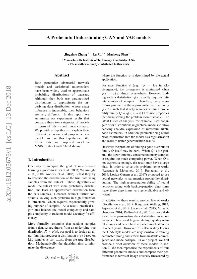
Figure 4. 10 handwritten images sampled from model (a)GAN (b)WGAN (c)VAE (d)VAE-GAN, the labels under eachrow of images are predicted by a well-trained two-layer fully-connected neural network classifier.

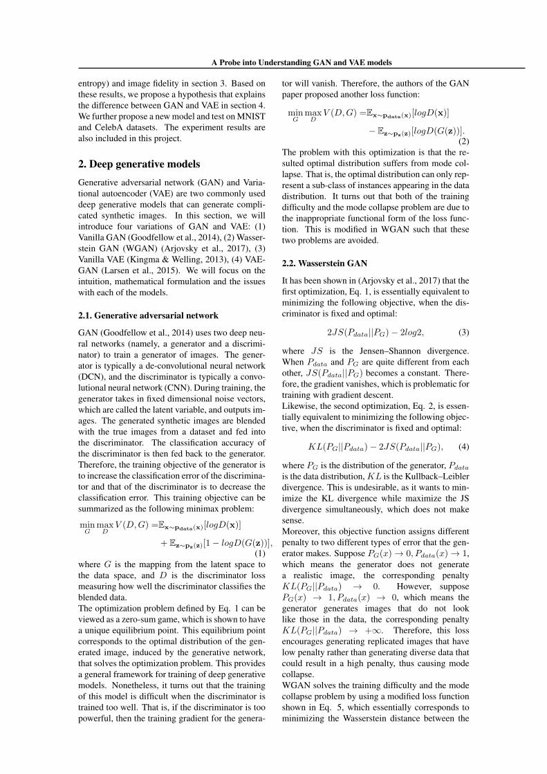
Figure 5. The single image entropy of each handwrittenimage in Fig.4 computed from the prediction probabilityof a pre-trained classifier. A low entropy means that theimage quality is high as it suggests that the classifier rec-ognizes the image easily. The x axis label represents theindex of each image generated from different models.

ation. We use the empirical estimator

pi =number images classified as digit i

number of images generated in total

Then the entropy of the generator can be estimatedas

Entropy = −10∑i

pi × log(pi)

When mode collapse happens, the entropy willkeep decreasing. For example, we show the training

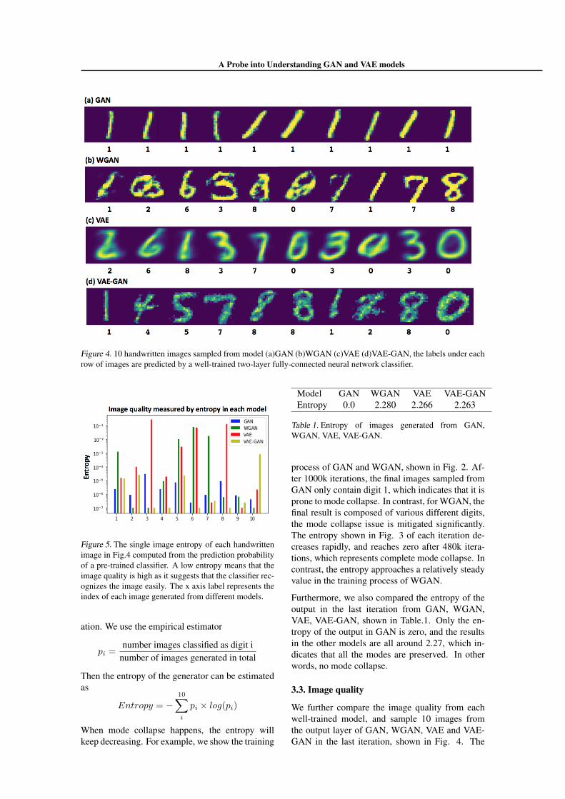
Model GAN WGAN VAE VAE-GANEntropy 0.0 2.280 2.266 2.263

Table 1. Entropy of images generated from GAN,WGAN, VAE, VAE-GAN.

process of GAN and WGAN, shown in Fig. 2. Af-ter 1000k iterations, the final images sampled fromGAN only contain digit 1, which indicates that it isprone to mode collapse. In contrast, for WGAN, thefinal result is composed of various different digits,the mode collapse issue is mitigated significantly.The entropy shown in Fig. 3 of each iteration de-creases rapidly, and reaches zero after 480k itera-tions, which represents complete mode collapse. Incontrast, the entropy approaches a relatively steadyvalue in the training process of WGAN.

Furthermore, we also compared the entropy of theoutput in the last iteration from GAN, WGAN,VAE, VAE-GAN, shown in Table.1. Only the en-tropy of the output in GAN is zero, and the resultsin the other models are all around 2.27, which in-dicates that all the modes are preserved. In otherwords, no mode collapse.

3.3. Image quality

We further compare the image quality from eachwell-trained model, and sample 10 images fromthe output layer of GAN, WGAN, VAE and VAE-GAN in the last iteration, shown in Fig. 4. The


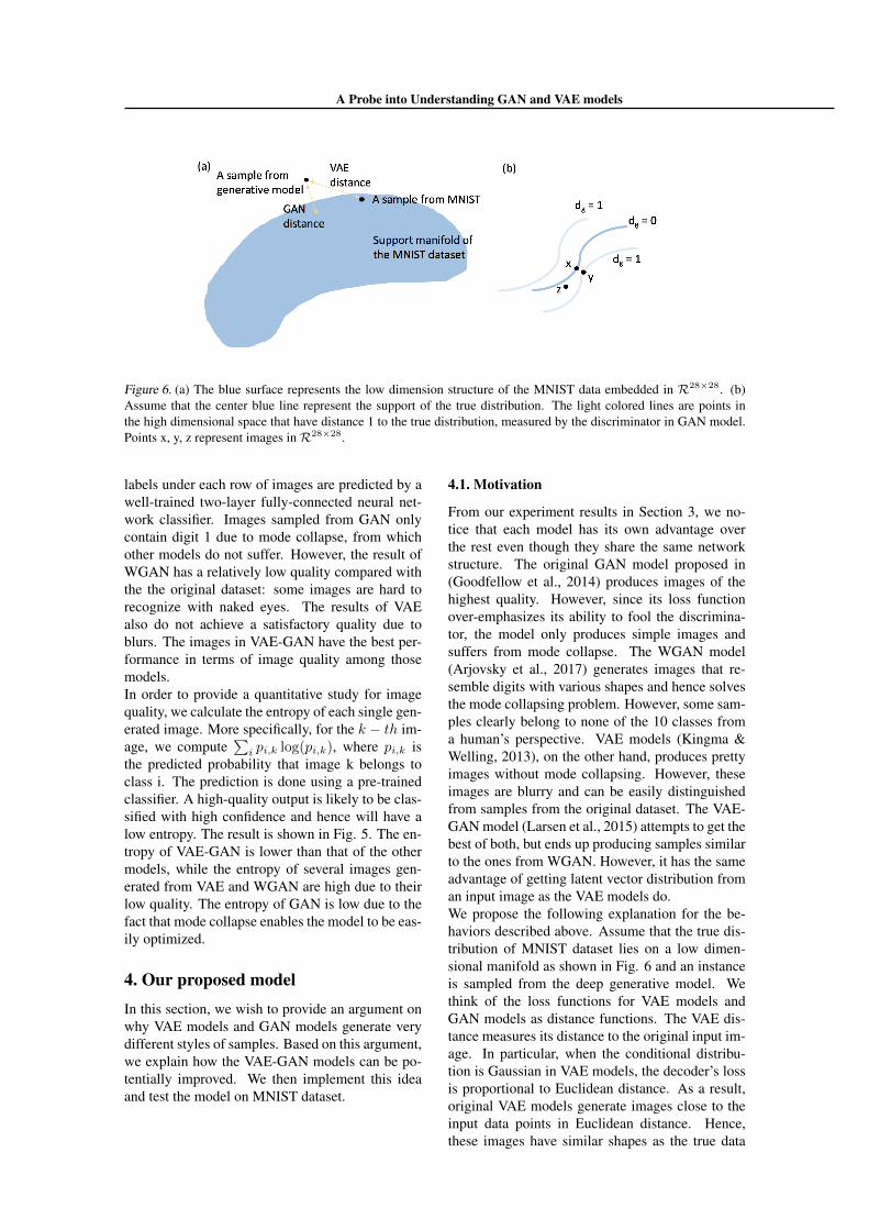
Figure 6. (a) The blue surface represents the low dimension structure of the MNIST data embedded in R28×28. (b)Assume that the center blue line represent the support of the true distribution. The light colored lines are points inthe high dimensional space that have distance 1 to the true distribution, measured by the discriminator in GAN model.Points x, y, z represent images inR28×28.

labels under each row of images are predicted by awell-trained two-layer fully-connected neural net-work classifier. Images sampled from GAN onlycontain digit 1 due to mode collapse, from whichother models do not suffer. However, the result ofWGAN has a relatively low quality compared withthe the original dataset: some images are hard torecognize with naked eyes. The results of VAEalso do not achieve a satisfactory quality due toblurs. The images in VAE-GAN have the best per-formance in terms of image quality among thosemodels.In order to provide a quantitative study for imagequality, we calculate the entropy of each single gen-erated image. More specifically, for the k − th im-age, we compute

∑i pi,k log(pi,k), where pi,k is

the predicted probability that image k belongs toclass i. The prediction is done using a pre-trainedclassifier. A high-quality output is likely to be clas-sified with high confidence and hence will have alow entropy. The result is shown in Fig. 5. The en-tropy of VAE-GAN is lower than that of the othermodels, while the entropy of several images gen-erated from VAE and WGAN are high due to theirlow quality. The entropy of GAN is low due to thefact that mode collapse enables the model to be eas-ily optimized.

4. Our proposed modelIn this section, we wish to provide an argument onwhy VAE models and GAN models generate verydifferent styles of samples. Based on this argument,we explain how the VAE-GAN models can be po-tentially improved. We then implement this ideaand test the model on MNIST dataset.

4.1. Motivation

From our experiment results in Section 3, we no-tice that each model has its own advantage overthe rest even though they share the same networkstructure. The original GAN model proposed in(Goodfellow et al., 2014) produces images of thehighest quality. However, since its loss functionover-emphasizes its ability to fool the discrimina-tor, the model only produces simple images andsuffers from mode collapse. The WGAN model(Arjovsky et al., 2017) generates images that re-semble digits with various shapes and hence solvesthe mode collapsing problem. However, some sam-ples clearly belong to none of the 10 classes froma human’s perspective. VAE models (Kingma &Welling, 2013), on the other hand, produces prettyimages without mode collapsing. However, theseimages are blurry and can be easily distinguishedfrom samples from the original dataset. The VAE-GAN model (Larsen et al., 2015) attempts to get thebest of both, but ends up producing samples similarto the ones from WGAN. However, it has the sameadvantage of getting latent vector distribution froman input image as the VAE models do.We propose the following explanation for the be-haviors described above. Assume that the true dis-tribution of MNIST dataset lies on a low dimen-sional manifold as shown in Fig. 6 and an instanceis sampled from the deep generative model. Wethink of the loss functions for VAE models andGAN models as distance functions. The VAE dis-tance measures its distance to the original input im-age. In particular, when the conditional distribu-tion is Gaussian in VAE models, the decoder’s lossis proportional to Euclidean distance. As a result,original VAE models generate images close to theinput data points in Euclidean distance. Hence,these images have similar shapes as the true data


Figure 7. (a) Images sampled from VAE-GAN after training on the MNIST dataset. (b) Images sampled from ourproposed model after training on the MNIST dataset. (c) Generated images from VAE-GAN after training 25 epochson the CelebA dataset. (d) Generated images from constrained VAE-GAN after training 25 epochs on the CelebAdataset.

but admit small deviations in pixel values and areblurry. On the other hand, GAN distance mea-sures the fake point’s distance to the manifold, andequals zero as long as the point is on the mani-fold. Therefore, the GAN models produce pointsthat are very close to the true distribution’s support.However, without regularization based on the truedata points, these generated images may not spanthe entire manifold. Furthermore, the discriminatorlearned may not properly compute the distance dueto the difficulty of non-convex optimization.As explained in section 2.4, the VAE-GAN modeltries to optimize both loss functions at the sametime. The loss for the decoder and encoder can bewritten into two components as follows,

Lvae−gan(x) = Lgan(x) + Lvae

Yet, the result suggests that the GAN loss mightdominate the other since it strengthens over itera-tions. We wish to design a model that allows VAEloss to take effect. Hence, we propose a constrainedloss

minxLvae(x), s.t. Lgan(x) ≤ d

The justification for this model is illustrated in Fig.6. If point x is the input image. Then point z hasa lower loss in the original VAE-GAN model dueto its low GAN loss, but y would have a lower lossin our constrained model, since it is in the feasibleregion and has a lower VAE loss. Solving this con-strained problem allows the model to focus on imi-tating the shape of the original data samples as long

as the image quality can almost fool the discrimina-tor. In order to solve this constrained problem, werewrite it in its Lagrangian form

L(λ, x) = Lvae(x) + λ(Lgan(x)− d) s.t. λ ≥ 0

By KKT conditions, we can find local optima bysolving L(λ∗, x), where λ∗ that maximize L(λ, x).It is straightforward to check that λ∗ = 0 whenLgan(x) ≤ d, and λ∗ =∞ when Lgan(x) > d. Asan approximation, we solve the following problemfor a fixed λ > 0,

minx

[Lvae(x) + λmax{Lgan(x)− d, 0}]

The sub-gradient for this loss function can be easilycomputed and we can train the neural network withback-propagation as usual.

4.2. Experiment

The only difference between our model and theVAE-GAN model is that it uses a nonlinear combi-nation of the loss from the VAE model and the lossfrom the discriminator. Hence, to control all otherfactors, we only changed the loss function in ouroriginal code for training VAE-GAN models, andran stochastic gradient descent algorithm for thesame number of iterations.

First, we run both models on MNIST dataset. Bothmodels use the same 5-layer fully connected neuralnetworks as introduced in Section 3. The sampledrandom images are shown in fig. 7(a)(b). Neither of


Figure 8. We sample 10k images from both constrainedvaegan and vaegan models. We then use a pretrainedclassifier to classify each single image. For every image,we can compute its own entropy using predicted proba-bility for each class. A high quality image can be recog-nized easily and hence should have low entropy.

the two models has a dominating performance, butour proposed one seems to have more stable imagequality. This is verified in fig. 8. The entropy hereis defined the same way as the entropy in fig. 5.Low entropy is associated with high image quality.We notice that our proposed algorithm has higherconcentration of low entropy images compared tothe original VAEGAN model.Then we tested both models on the CelebA datasetwith convolutional neural networks. Our networkarchitecture has three convolution layers and is thesame as the original paper in (Larsen et al., 2015).The original code runs the training process forabout 50 epochs, but due to our limited computationresource, we have to terminate the process at epoch25 after training for an entire week. Some prelim-inary results are shown in fig. 7(c)(d). We are notable to draw any interesting conclusion since thenetwork has not converged.

5. DiscussionThere are a few problems unsolved due to our lim-ited time and computation resource. First, MNISTis a dataset with a simple structure. Therefore, theconclusions we draw based on MNIST experimentsmay not generalize to more complicated data. Eventhough we attempt to train some convolutional neu-ral networks(CNN) on the CelebA data set, the lackof GPU access forces us to terminate the experi-ment before it finishes training. Therefore, it wouldbe interesting to check if our proposed model canhave greater improvement when the manifold inhigh dimensional space is more complicated. Sec-ond, the quality of the images generated in our ex-periments are relatively low compared to results inmore recent literatures. This results from the dis-advantage of fully connected neural network com-

pared with CNN in learning image structures. Wesuspect that our WGAN model generates low qual-ity images because the network is not powerfulenough. Again, we do not have enough resources toconduct experiments that require convolution oper-ations.In the results shown, we tried to make fair compari-son by using the same network architecture in all ofour models. We trained VAE-GAN and constrainedVAE-GAN with the same parameters for the samenumber of iterations. Other models are trained un-til the image quality stabilizes. From these re-sults, we may conclude that our explanation in insection 4 aligns with the experiments in Section3. However, the experiment comparing VAE-GANand constrained VAE-GAN shows little difference,and more efforts are needed before we could getstronger evidence to support our claim.

ReferencesAndrieu, Christophe, De Freitas, Nando, Doucet,

Arnaud, and Jordan, Michael I. An introductionto mcmc for machine learning. Machine learn-ing, 50(1-2):5–43, 2003.

Arjovsky, Martin, Chintala, Soumith, and Bot-tou, Léon. Wasserstein gan. arXiv preprintarXiv:1701.07875, 2017.

Blei, David M, Ng, Andrew Y, and Jordan,Michael I. Latent dirichlet allocation. Journalof machine Learning research, 3(Jan):993–1022,2003.

Goodfellow, Ian, Pouget-Abadie, Jean, Mirza,Mehdi, Xu, Bing, Warde-Farley, David, Ozair,Sherjil, Courville, Aaron, and Bengio, Yoshua.Generative adversarial nets. In Advances in neu-ral information processing systems, pp. 2672–2680, 2014.

Kingma, Diederik P and Welling, Max. Auto-encoding variational bayes. arXiv preprintarXiv:1312.6114, 2013.

Larsen, Anders Boesen Lindbo, Sønderby,Søren Kaae, Larochelle, Hugo, and Winther,Ole. Autoencoding beyond pixels using alearned similarity metric. arXiv preprintarXiv:1512.09300, 2015.

Loaiza-Ganem, Gabriel, Gao, Yuanjun, and Cun-ningham, John P. Maximum entropy flow net-works. arXiv preprint arXiv:1701.03504, 2017.

Mirza, Mehdi and Osindero, Simon. Condi-tional generative adversarial nets. arXiv preprintarXiv:1411.1784, 2014.

Radford, Alec, Metz, Luke, and Chintala, Soumith.Unsupervised representation learning with deep


convolutional generative adversarial networks.arXiv preprint arXiv:1511.06434, 2015.

Ranganath, Rajesh, Tran, Dustin, and Blei, David.Hierarchical variational models. In InternationalConference on Machine Learning, pp. 324–333,2016.

Rezende, Danilo Jimenez and Mohamed, Shakir.Variational inference with normalizing flows.arXiv preprint arXiv:1505.05770, 2015.

Wainwright, Martin J, Jordan, Michael I, et al.Graphical models, exponential families, andvariational inference. Foundations and Trends R©in Machine Learning, 1(1–2):1–305, 2008.

a probe into understanding gan and vae models

Documents