a procedure for estimating the unconditional … · appl statist. (1994) 43, no. 4, pp. 599-624 a...

Appl Statist. (1994) 43, No. 4, pp. 599-624

A Procedure for Estimating the Unconditional Cumulative Incidence Curve and Its Variability for the Human Immunodeficiency Virus By JOEL W. HAY

University of Southern California, Los Angeles, USA

and FRANK A. WOLAKt

Stanford University, USA

[Received December 1991. Revised October 1993]

SUMMARY A backcalculation procedure is presented for estimating both the cumulative incidence of the human immunodeficiency virus (HIV)-the total number of seropositive individuals as a function of calendar time-and the unconditional sampling distribution of this estimate. This estimation framework explicitly accounts for corrections for reporting lags in the most recent AIDS diagnosis data and imposes no functional form restrictions, besides a roughness penalty, on the resulting estimate of the cumulative incidence function. The construction of the sampling distribution for this estimate 'integrates out' the variation due to the use of estimated reporting lag and incubation distributions to obtain the unconditional distribution. The estimation procedure amounts to solving an inequality-restricted generalized least squares estimation problem subject to smoothness priors on the regression coefficients. We find that both the point estimate of the cumulative incidence curve for HIV and its associated upper and lower confidence bound paths remain stable over a wide range of estimation scenarios. In addition, not accounting for the use of estimated incubation and reporting lag distributions in the procedure for estimating the cumulative incidence curve can lead to a substantial underestimation of its sampling variability.

Keywords: Confidence intervals for cumulative human immunodeficiency virus incidence curve; Human immunodeficiency virus incidence; Inequality-restricted regression; Multistage bootstrap sampling distribution; Smoothness priors

1. Introduction

This paper presents a backcalculation procedure, similar to those described in Becker et al. (1991), Brookmeyer (1991), Brookmeyer and Gail (1988), Rosenberg and Gail (1990, 1991) and Harris (1990), for estimating the cumulative incidence curve for human immunodeficiency virus (HIV, or HIV type 1). Our procedure yields a point estimate of the incidence curve for HIV-the total number of seropositive individuals as a function of calendar time-which takes into account

tAddress for correspondence: Department of Economics, Stanford University, Stanford, CA 94305, USA. E-mail: [email protected]

? 1994 Royal Statistical Society 0035-9254/94/43599

600 HAY AND WOLAK

uncertainties in the reporting lag and incubation distribution and imposes no functional form restrictions, besides a roughness penalty. The primary goal of the paper is to provide an estimate of the unconditional sampling distribution of this point estimate which is consistent with our estimation procedure so that confidence bound paths for our cumulative incidence curve estimate can be computed.

HIV and the acquired immune deficiency syndrome (AIDS) have had a substantial effect on providing and financing health care over the past decade. Up to December 1992, the Centers for Disease Control (CDC) has reported 249199 cases of AIDS in the USA and 169623 AIDS-related deaths (Centers for Disease Control, 1993). Also, new forms of therapy are substantially increasing the average cost of medical care per patient lifetime (Hay et al., 1991). To make informed policy decisions about future AIDS costs and resource utilization, both a point estimate for the cumulative HIV incidence curve and its associated unconditional sampling distribution are necessary to derive base-line, best case and worst case policy scenarios for the time path of future AIDS diagnoses in the USA.

Following the presentation of our estimation procedure, we discuss how to use our cumulative incidence curve and its sampling distribution to compute a point estimate and associated confidence intervals for future AIDS diagnoses. Medley et al. (1991) and Brookmeyer (1991) also presented methodologies for constructing point estimates and confidence intervals for the future time path of AIDS diagnoses. Knowledge of these upper and lower confidence bounds will allow health policy makers to build into the health care delivery process the flexibility necessary to deal with the contingencies contained within these bounds.

To clarify our estimation procedure, we first describe the three sources of error in the observed diagnosis data. The first source is due to the delay between the time that an AIDS case is diagnosed and when it is reported to the CDC. Consequently, the more recently reported AIDS diagnosis totals must be inflated to reflect this reporting lag. This inflation process introduces measurement error which we control for in our backcalculation procedure. In addition, we must use an estimate of the reporting lag distribution to construct these inflation factors. We allow for this increased variability in the calculation of the confidence interval paths for our cumulative incidence curve estimate.

All backcalculation estimation procedures rely on an estimate of the AIDS incubation distribution, i.e. the time from HIV seroconversion to diagnosis of AIDS. Incubation distribution estimates are usually obtained from prospective studies of specific samples of high risk populations. In the construction of our confidence bound paths, we control for the additional source of variability introduced by using an estimated incubation distribution rather than the true incubation distribution.

The third source of error is uncertainty in the incubation time. Even if we assume that the incubation distribution is known, for any individual the time between seroconversion and diagnosis of AIDS is a random variable with this known distribution. Ignoring, for the moment, the first two sources of error, there is still residual uncertainty concerning the exact number of seropositive people in the population because of the uncertainty about the time between infection and diagnosis. Our estimation procedure takes into account all three sources of uncertainty in estimating the cumulative HIV incidence curve and its confidence bound paths.

ESTIMATING CUMULATIVE INCIDENCE CURVE 601

One outcome of our empirical results is a demonstration that failing to account for the use of estimated reporting lag and incubation distributions can substantially understate the variability in a cumulative HIV incidence estimate.

Our procedure has several attractive features which we summarize here. First, the procedure does not require a specific distributional or functional form assumption for the reporting lag distribution estimation and correction procedure. Many of the available reporting lag correction procedures can be built into this estimation framework. For example, the procedures suggested by Harris (1990), Brook- meyer and Damiano (1989), Brookmeyer and Liao (1990), Zeger et al. (1989) and Rosenberg (1990) can, with varying computational effort, be integrated into this backcalculation procedure. The estimation procedure is also flexible to the form of the assumed incubation distribution; no functional form or distributional restriction is required. As long as an estimate of the sampling distribution of this incubation distribution estimate is available, our procedure will utilize this information to control for both the form and the variability in the assumed incubation distribution. Other than smoothness restrictions, our procedure imposes no functional form restrictions on the cumulative incidence curve. Finally, our procedure explicitly accounts for the discrete nature of the CDC data. For each observation in the CDC public information data set (Centers for Disease Control, 1991), only the month and year of the report date and diagnosis date are given. This estimation procedure allows the researcher to use precisely this level of time aggregation in computing an estimate of the cumulative HIV incidence curve.

We consider various estimation scenarios to assess the effect of several of our modelling assumptions. First are the assumptions made about the AIDS incubation distribution during the first two years since seroconversion. As is well documented, an HIV-infected individual rarely progresses to AIDS in the first 24 months following infection (Bacchetti, 1990; Bacchetti and Moss, 1989; Brookmeyer and Goedert, 1989; Hessol et al., 1989; Mufioz et al., 1989). Our modelling strategy deals with this very low probability of early progression to AIDS in various ways.

Another distinction between our scenarios is the time period of analysis. We perform our estimation over two different sample periods:

(a) a long sample - from 1979 to the middle of 1990- and (b) a short sample - from 1979 to the third quarter of 1987.

The short sample ends before therapy, particularly the use of zidovudine and aerosol pentamidine, became indicated for AIDS treatment and thus potentially altered the HIV incubation distribution. A comparison of seroconversion totals estimated up to 1987 for both samples provides some insight into the debate between therapy versus slowing down in the number of infections as the cause of the recent levelling off of the monthly total AIDS case diagnoses (Gail et al., 1990).

The point estimates of the cumulative incidence curve for both the long and the short samples are quite stable across the many estimation scenarios that we consider. For the long sample, we find that up to mid-1990 the cumulative number of seropositive cases is approximately 670000, with a 95%o confidence interval from approximately 500000 to 850000. For the short sample, we find a total up to the third quarter of 1987 of 980000 with a 95%o confidence interval of approximately 600000-1300000. More diffuse smoothness priors only slightly increase the size of the confidence interval estimates; tighter priors decrease the size of the confidence

602 HAY AND WOLAK

intervals. These confidence intervals are for values of the smoothness prior which impose what we believe to be a small amount of smoothing on the estimated cumulative incubation function.

The remainder of the paper is devoted to explaining our backcalculation and unconditional confidence path estimation procedure. We then summarize the results of our experience with the many different modelling scenarios used to assess the durability of our estimation results. The next section discusses the procedures that we use to adjust the recent AIDS diagnosis data totals for reporting lags. Section 3 presents the statistical model used to estimate the cumulative HIV incidence curve under the assumption that the diagnosis totals for all time periods in the sample are measured without error. Section 4 details the adjustments to our statistical model and estimation procedure that are necessary to take into account errors introduced by the reporting lag correction procedure. Section 5 discusses the form of the smoothness priors imposed on the estimated cumulative incidence curve and the corrections made to the incubation distribution hazard rate for the first 24 months after infection. Section 6 outlines our procedure for computing an estimate of the unconditional sampling distribution of the cumulative HIV incidence curve and describes several procedures for constructing its associated confidence bounds. Section 7 summarizes the results of the estimation scenarios and presents what we believe is the most plausible cumulative incidence function estimates for our data set. In this section we quantify the additional variability in the cumulative incidence estimates which is caused by the use of estimated reporting lag and incubation distributions. Section 8 outlines how this cumulative incidence estimate and associated sampling distribution can be used to predict future diagnoses of AIDS. The final section discusses directions for future research.

2. Reporting Delay Adjustment Procedure for Acquired Immune Deficiency Syndrome Cases

There are two determinants of AIDS case underreporting. First, diagnosed AIDS cases are reported to the CDC with a stochastic lag. Second, some portion of AIDS cases are never reported to the CDC. The CDC estimates that 150o of all AIDS cases are permanently unreported (Centers for Disease Control, 1990). A recent study by Rosenblum et al. (1992) found less underreporting: between 100o and 5/o. Rather than to attempt to account for this second source of underreporting in our sample, we instead present our results assuming the existence of only the first source of underreporting error. Even if the fraction of unreported cases is assumed fixed for all time periods in our sample, correcting for this second source of underreporting will have a non-linear, rather than simply a proportional, effect on the estimated time path of HIV incidence. Because of the uncertainty associated with the true proportion of unreported cases for each month in our sample, we instead focus on estimating the cumulative incidence curve only for those infections that will be reported when diagnosed.

The first step in Rosenberg's (1990) procedure is to construct the analogue to Table 1 given in his paper. Our data set is diagnoses of AIDS in all adults and adolescents for the USA up to the second quarter of 1990. Table 1 contains our version of Rosenberg's Table 1. Our table differs from Rosenberg's in two respects. First we assume that no reporting lag is longer than 4 years, rather than the 3

TABLE 1 Calendar period of diagnosis versus reporting delay in months for US AIDS cases reported to the CDCt

Diagnoses No. of cases for the following reporting delays in months: Total Imputed period 0 1-3 4-6 7-9 10-12 13-15 16-18 19-21 22-24 25-27 28-30 31-33 34-36 37-39 40-42 43-45 46+ total

Year Quarter

1982 1 31 49 32 10 5 10 5 2 4 0 2 0 0 0 0 0 35 185 185 1982 2 40 67 11 5 10 9 7 3 0 2 1 3 1 0 1 0 41 201 201 1982 3 78 73 32 21 12 11 1 3 1 2 2 1 1 1 2 2 50 293 293 1982 4 96 129 30 33 17 5 2 3 1 0 2 3 1 0 0 1 58 381 381 1983 1 134 177 68 34 14 12 4 7 4 3 4 2 1 2 0 67 536 53681 1983 2 57 378 85 43 20 18 12 9 5 6 5 0 5 5 2 3 52 705 705 > 1983 3 69 420 113 34 19 12 10 10 4 4 3 4 3 3 7 4 50 769 769 1983 4 26 513 109 55 25 17 7 8 4 3 7 9 8 7 5 0 48 851 851 z 1984 1 55 675 151 59 32 26 18 8 9 7 7 4 9 7 5 6 70 1148 1148 1984 2 82 790 164 85 57 36 16 4 11 9 6 12 9 11 5 11 65 1373 1373 1984 3 108 845 241 112 47 40 18 16 15 9 8 8 5 13 11 7 70 1573 1573 1984 4 118 960 247 112 65 30 27 15 11 1985 1 146 1191 252 129 83 67 34 20 18 22 15 18 22 27 29 21 68 2157 2157 4 1985 2 160 1454 292 143 93 58 48 35 24 20 29 46 33 31 23 27 62 2578 2578 1985 3 152 1620 400 225 101 71 53 39 20 56 55 44 29 -35 22 21 54 3997 2997 1985 4 97 1739 422 164 120 58 52 52 57 65 83 41 37 27 29 17 47 3107 3107 1986 1 148 2046 406 218 107 118 56 107 135 102 813 9 3 40 26 30 53 3775 31077 1986 2 362 2039 555 200 143 91 152 160 133 94 77 66 41 31 27 38 54 4263 4263 z 1986 3 232 2444 532 275 148 196 229 165 123 80 62 58 36 42 39 31 11t 4692 4862 1986 4 181 2441 763 290 240 282 183 143 101 82 67 35 38 50 39 8t 0 4935 5152 1987 1 224 2981 673 408 370 353 224 185 99 126 85 85 78 56 20 0 0 5947 6256 Z 1987 2 129 3260 897 592 426 272 193 125 133 121 91 96 74 9t 0 0 0 6409 6806 1987 3 96 3567 1207 569 374 227 156 138 102 118 117 85 19t 0 0 0 0 6756 7249 1987 4 135 3847 1218 444 315 247 195 128 149 140 102 21t 0 0 0 0 0 6920 7519 1988 1 163 4401 1096 462 354 334 196 186 203 140 102 01 0 0 0 0 0 7690 7519 1988 2 307 4608 968 500 372 284 225 231 182 516 0 0 0 0 0 0 0 7677 8628 1988 3 332 4521 1186 569 334 317 222 193 63t 0 0 0 0 0 0 0 0 7674 8808 t 1988 4 256 4525 1327 487 375 387 268 88t 0 0 0 0 0 0 0 0 0 7625 8975 1989 1 311 5016 1248 569 527 438 82t 0 0 0 0 0 0 0 0 0 0 8109 9843 1989 2 342 5186 1370 814 512 146t 0 0 0 0 0 0 0 0 0 0 0 8224 10443 1989 3 349 5124 1515 830 188t 0 0 0 0 0 0 0 0 0 0 0 0 7818 10511 1989 4 192 4998 1745 272t 0 0 0 0 0 0 0 0 0 0 0 0 0 6935 10206 1990 1 276 5646 706t 0 0 0 0 0 0 0 0 0 0 0 0 0 0 5922 10898 1990 2 329 2092t 0 0 0 0 0 0 0 0 0 0 0 0 0 0 0 329 9187

Total June 1986-June 1990 132170 162321 133683

tAdapted from Rosenberg (1990). 8 tCells with incomplete data because of reporting delays. w

604 HAY AND WOLAK

years that he assumes. (Although some AIDS cases have reporting lags of 5 years or longer from the time of diagnosis, they are quite uncommon. Some experimentation with allowing longer maximum reporting lags led to barely noticeable changes in our results.) In addition, we use only data after the first quarter of 1982 to estimate the reporting lag distribution. Following Rosenberg, let Rl9, . . ., R34 denote the row sums of Table 1 corresponding to the third quarter of 1986 until the second quarter of 1990 and Yl9, . . ., Y34 denote the unobserved actual number of cases diagnosed in these periods. The Ri and Yi are related by the reporting lag distribution pj (j=O, 1, . . ., 16), where pj denotes the probability that a case diagnosed in quarter t is reported in quarter t+j, and E> tp1= 1, because of our assumption that no reporting lag is longer than 4 years.

Rosenberg's estimation procedure produces maximum likelihood (ML) estimates of the parameters f0, P1, . . *, P under the modelling assumptions given in Brookmeyer and Damiano (1989) which assume a stationary reporting lag distribution. (Work by Harris (1990) and Brookmeyer and Liao (1990) provides evidence against this assumption.) The Yi are estimated by multiplying the observed R, (i=19, 20, .. ., 34) by the inflation factor (PO+P1+ +P34-i)-1 The last column of Table 1 contains our actual totals for the period between the first quarter of 1982 and the second quarter of 1986 and the imputed totals from the third quarter of 1986 until the second quarter of 1990. This column of estimated AIDS diagnoses and the quarterly diagnoses totals from the first quarter of 1979 to the last quarter of 1981 are used to compute our point estimate of the cumulative HIV incidence curve.

3. Statistical Model of Acquired Immune Deficiency Syndrome Infection Distribution

Our statistical procedure approximates the cumulative HIV incidence curve by a step function which has as many steps as there are time periods for observed AIDS diagnosis data and in this sense imposes no functional form restrictions. We impose our a priori restrictions in the form of smoothness priors on the parameters deter- mining the step function. We discuss these smoothness priors after the descrip- tion of the estimation procedure for the case of reporting lag-correction-induced measurement error.

For estimation purposes our time period of observation is a quarter of a year; however, the model allows the selection of any discrete time period as the unit of observation. Because the CDC data have been reported monthly, for all practical purposes the minimum unit of observation is 1 month. Preliminary experimentation indicated very little difference in the results across monthly and quarterly levels of aggregation. To reduce computational time substantially we use quarters as the time period of analysis.

First we define the following notation. Let Yt denote the number of AIDS cases diagnosed in quarter t. Let xti denote the probability that an individual who sero- converts in quarter i is diagnosed with AIDS in quarter t. Both i and t are indices running from 1 to T, the total number of quarters in our sample, with T denoting the most recent quarter (the second quarter of 1990) and t = 1 the most distant quarter (the first quarter of 1979). These xti are derived from an estimated AIDS incubation distribution. (This procedure does not require the incubation distribution


to be stationary (independent of calendar time), because xti is explicitly indexed by both the time of infection and the time of diagnosis, not by the difference between the two as is required for stationarity. Although the incubation distribution used in our empirical analysis assumes stationarity, the AIDS incubation distribution may have changed (Taylor et al., 1991; Gail et al., 1990) because of the recent wide- spread use of therapy. This form of non-stationarity could be accounted for by computing different xj for different infection times.) Let 1i denote the number of individuals seroconverting in quarter i (i = 1, . . ., T).

According to our model, the observed pattern of AIDS case diagnoses arises in the following way. Let zti denote the number of individuals who seroconvert in quarter i who then are diagnosed with AIDS in quarter t. Let Zi = (zTij Z(T- 1)ij ... IzZ1)'. (We follow the standard convention that all vectors are column vectors.) Using this notation define Z4* = (Z(t T)i, Zi')', where Z(t> T)i denotes the sum of all individuals who seroconvert in period i and are diagnosed with AIDS in all periods t > T. Under the assumptions of our model, we have the following result: Z4* has a multinomial distribution with parameters (1 - IT=1Xti XTi, X(T- 1)i

.. ., xii) and fi. Consequently, our model of the AIDS infection process assumes that Oi individuals seroconvert each quarter during our sample and then progress to AIDS in the current and succeeding quarters according to a multinomial distribution derived from the AIDS incubation distribution relevant for seroconversions occurring in the ith quarter (i = 1, . . ., T). Because the probability of progression to AIDS for an individual seroconverting in quarter i is independent of that same probability for an individual seroconverting in any other quarter, the Z4* are independent draws from known multinomial distributions conditional on the xi (i=l, . ., T) (t=1, . . ., T) and 1i (i=l, . . ., T).

Define the following vectors: Xi= (xTi, XTi, . .. ., xli)', Y= (YT, YT-1, I Yi)' and 3 = (fT, T-1, .. ., fI1)'. Let X= (XT, XT-1, .. ., X) denote the Tx T matrix of elements xti. (This construction of the X-matrix and Y-vector differs from the standard approach of putting the most distant observations in the first row and the most recent in the last row. However, our desire to retain chronological order in our time index t necessitated this counter-intuitive construction of the X-matrix and Y-vector.) In terms of this notation we have the result E,T=I Zi = Y. Consequently, Y, the realized value of the AIDS case diagnoses vector, is the sum of T independent multinomial random vectors. This implies the result

T T E(Y) = ZE(Zi) = ZXii = Xf. (1)

i=l ~~i=l

For the covariance matrix of Y (var(Y)), we have T T

var(Y) = E= E var(Zi) = j {diag(xT,xT i, i. .., xli) - XAX1'}fl, (2) i=l i=l

where diag(xTi, XTli . ., xh) is a Tx T diagonal matrix with X(T+ 1 -k)i as the diagonal element in the kth row and column. We have now characterized the first two moments of the AIDS diagnosis vector in terms of our statistical model. Note that, because a person cannot be diagnosed with AIDS before seroconverting, xti =0 for all i > t.

Our model can be written in the familiar linear regression form as

606 HAY AND WOLAK

Y = X: + e (3)

where e = (et, . . *, rT)' satisfies the following moment restrictions: E(e) = 0 and E(EE') = E. Conditional on the value of X, what we call the progression matrix, we can apply ordinary least squares (OLS) to obtain unbiased estimates of the elements of f. However, because of its interpretation as the number of new seroconversions in a given time period, a negative point estimate of fi makes no sense. To make our estimated statistical model biologically meaningful, we impose the restriction that all the elements of : are non-negative, so that 0 is the lower bound on the estimated number of seroconversions for each time period. In this way, our estimation procedure imposes the logical constraint that the step function approximating the cumulative HIV incidence curve can only remain the same or increase as time progresses.

Because the covariance matrix of the disturbance vector e is non-scalar, OLS will not yield the most efficient estimates. This form of our model should be estimated by a multistep generalized least squares (GLS) approach subject to inequality restrictions on all the elements of f. The first step estimates e by inequality-restricted least squares, to obtain &. (Liew (1976) discussed inequality-restricted least squares estimation. Bazaraa and Shetty (1979) discussed the computational aspects of constructing this estimator, which involves solving a quadratic program.) Using f0, EO, an estimate of E, is constructed by replacing : with 0 in equation (2). Using O, OG, the inequality-restricted GLS estimate of 3, is computed.

These two estimates of f are the solutions to the following two quadratic programming problems:

sup1{(Y-X13)'(Y-X3)} (4)

and

sup{i(Y - XO) E0 ( Y - X:)}. (5)

We then perform one further GLS iteration updating E using OG, which entails inequality-restricted GLS with ?G. Carroll et al. (1987) stated that there is little justification (in terms of efficiency gains) for updating beyond this estimate of E.

As discussed in Section 2, we do not observe the true Yt for the most recent 16 quarters. The use of reporting lag-corrected diagnosis data will induce measurement error into these Yt which will change the covariance matrix of the disturbance vector in the linear model used to estimate f. We now describe the properties of the measurement error induced by the data imputation techniques discussed in Section 2 and our procedure for correcting for its presence.

4. Estimation Technique with Reporting Lag Measurement Error

To assess the effect of the measurement error in Yt which results from using the reporting-lag-corrected diagnosis totals in the analysis, we must rewrite our regression model in the notation

Yt = X;:l + t (t=1, . . ., T) (6)


where X;' is the (T+ 1 - t)th row of the X-matrix defined earlier. Recall that the index t is defined as follows: t = 1 is the first quarter of 1979; t =2 is the second quarter of 1979; . . ., t = 46 = T is the second quarter of 1990. Recall from Section 2 that Pi is the estimated probability of a reporting lag of exactly i quarters and that pi is the true value of this probability. Define A, =E= Pr, so that A5 is the probability of a reporting lag of less than or equal to s quarters. Define ei such that eO = R34, el =R33, . . ., el5= R19, where Ri is as defined in Section 2. In terms of this notation, conditional on Yt (t = T, T- 1, . . ., T- 15), eT-t has a binomial distribution with parameters AT_t and Yt. Conditional on Yt the expectation of eT-t

iS AT- tYt and var(eT- t) =AT- t ( - AT- t)yt. Define ~true 7 yt = eTtAT-t (7)

If AT-t were measured without error, equation (7) would give the value of Yt used in our analysis. Because we estimate the reporting lag distribution, we must replace AT-t with our point estimate of ATt, which we denote AT-t, to compute

9t = eT-tIAT-t (t = T, T- 1, ... ., T- 15) . (8)

These are the estimated values of Yt used in our analysis. Replacing AT-t with AT-t to compute the estimated number of AIDS case

diagnoses for quarter t implies that any estimate of a obtained will be conditional on the value of AT-t used. Because of our desire to obtain the unconditional sampling distribution of the cumulative HIV incidence curve, we must control for the use of AT-t instead of AT-t in computing this unconditional sampling distribution.

Even if AT-t were known, the use of 9t rather than Yt to estimate the cumulative incidence curve introduces a measurement error in Yt for all observations which are corrected for the reporting lag. The logic for this claim is as follows. Treating AT_t as if it were ATt, .9t and Yt satisfy the equation 9t =Yt + nt, where E(qt IYt) = 0 and

E(72 Iyt) = 1 AT-t Yt. AT- t

These facts imply that the conditional expectation of qt given Xt is 0 and the conditional variance E(7 IX;) is {(1 - ATt)/AT_t}XX'. Let -q denote the T- dimensional vector whose first 16 elements are rt as defined above and the remaining elements are 0. Let D denote the Tx T diagonal matrix with E(t 2I Xt) (t = T, T- 1, ., T- 15) as the first 16 diagonal elements and zeros for the remaining diagonal elements. In this notation, our model which accounts for the measurement error in the most recent Yt takes the form

Y= X: + ?* (9)

where q* = tq + E, for e as defined in Section 3. In this notation Y is identical with Y except that its first 16 elements are 9t rather than Yt. For this model, the error term q* satisfies the following two conditional moment restrictions:

(a) E(-q* IX) = 0; (b) var(,q* IX) = Q = E + D.

608 HAY AND WOLAK

TABLE 2 Point estimate of reporting delay densityt

Reporting delay Probability Reporting delay Probability (quarter) (quarter)

0 0.0358 9 0.0168 1 0.5076 10 0.0138 2 0.1361 11 0.0116 3 0.0643 12 0.0096 4 0.0438 13 0.0090 5 0.0362 14 0.0074 6 0.0258 15 0.0070 7 0.0216 16 0.0351 8 0.0185

tRosenberg's (1990) estimation procedure for the data from the first quarter of 1982 to the second quarter of 1990.

Given an estimate of 1, we can compute an estimate of D in the same manner as used to construct an estimate of E. Consequently the inequality-restricted OLS followed by two rounds of inequality-restricted GLS estimation is identical with that described above with E replaced by D.

Before concluding this section, we should comment on the intuition embodied in our modified estimation procedure which takes into account the measurement error induced by the reporting lag correction. This correction introduces an additional independent heteroscedastic error into the more recent AIDS diagnosis observations. By inspection of var(f7, 1 Xt), the smaller A, is, the larger the variance of var(,qtjXt[). Table 2 presents the point estimates of the reporting lag probabilities. These imply a value of Ao = 0.0358. Inserting this value of Ao into the expres- sion for (1 - AO)/AO yields 29.39. In addition, Xt'f for t = T should be quite large. Therefore, the conditional variance of 71T will be a very large number, which indicates that YT will (as intuition requires) receive a very small weight in the GLS estimation of 1. By this same logic, the residuals from the more recent observations will be downweighted relative to those further in the past in the estimation of 3. This correction to the estimation procedure provides a model-based statistical rationale for data-dependent downweighting of more recently diagnosed AIDS cases due to the reporting lag correction procedure.

5. Additional Information Used in Estimation

In this section we discuss various sets of restrictions placed on the form of the cumulative incidence curve. All these restrictions take the form of smoothness priors on the shape of the curve. We impose these priors for the following reasons. Incubation distribution estimation techniques exist which yield 0 or values very close to 0 as the point estimate of the hazard rate for the AIDS incubation distribution during the first several months following seroconversion (e.g. Bacchetti (1990)). (These low hazard rate estimates are consistent with the well-known low probability of progression to AIDS within the first 24 months following seroconversion.) Consequently, the most recent O's cannot be identified, or identified with


any precision, without further assumptions. By imposing smoothness priors on the relationship between the elements of : over the entire sample we can overcome this problem.

Selecting the degree of smoothness for the cumulative incidence curve is an extremely difficult task. Here the researcher's prior beliefs explicitly enter the analysis. We now try to motivate our specific selections for the smoothness prior. In Section 7, we examine the sensitivity of the results to our choices. We consider two types of smoothness prior. Both can be written in the generic form

0 = Rf + v, (10)

where v is a Tx T random variable with mean 0 and diagonal covariance matrix kIT (IT is a Tx T identity matrix and k is a positive scalar) and R is a square matrix which depends on the type of smoothness restrictions imposed. The two sets of restrictions that we consider are first-difference and second-difference restrictions. By first-difference restrictions we mean that the successive differences between fl and fl -l have mean 0 and variance k. In this case R has a 1 in the (i, i) position and -1 in the (i, i + 1) position for i = 1, 2, ..., T. The remaining elements of R are 0.

The second-difference constraint imposes prior information on the successive differences of the first differences:

t - t-1 - (t-1 - Ot-2)* (11) In this case the R-matrix has 1 in the (i, i) element -2 in the (i, i + 1) element and 1 in the (i, i+ 2) element, i = 1, 2, . . ., T. The remaining elements of R are set to 0.

The tightness of the prior is determined by the value of k in the covariance matrix of v. If we are willing to assume that v is close to a Gaussian distribution, we can make informal probabilistic statements about the degree of confidence that we have in our prior. For example, by the properties of the normal distribution there is a 95 %o probability that v lies in the interval [ - 1.96k112, 1.96k112]. Once we have selected a form for R, using this 95'0o probability interval for each element of v, and our beliefs about the likely variability in the magnitudes of the first differences and second differences in the ft, we can select an appropriate value for k.

Once k and R have been selected we repeat our inequality-restricted combination OLS and GLS procedure to compute estimates of from the Theil and Goldberger (1961) stacked mixed regression model

(0) (R + ( v ) (12)

in the same manner as described earlier. The first step computes the least squares estimates of : imposing the smoothness prior and the second stage computes an estimate of Q based on the OLS estimate of : and utilizes this covariance matrix estimate to apply GLS with the smoothness prior. The final iteration computes an estimate of Q from the GLS estimate of : and then re-estimates f by GLS imposing the smoothness prior. Experimentation with further iterations of Q0 and :- yielded very little change in either the point estimates of : or the estimate of its sampling distribution.

The OLS and GLS procedures involve the solution of the following two quadratic programming problems:

610 HAY AND WOLAK

sup {-2 Y'Xo + a3'(X'X + k 1R'R)j } (13)

and sup { -2Y' -X3 + fl'(X''X - 1X + k - 1R'RR)} (14)

where Q is the estimate of Q that is appropriate for that round of the estimation. Because of the Os in the estimated hazard rate, the estimated Q will, in general, be positive semidefinite. In these instances we can use the generalized inverse of Q in the GLS estimation.

An alternative procedure which imposes additional prior information to solve the problem of singular X'X and Q matrices involves assuming a minimum base-line hazard for progression to AIDS in the first 2 years since seroconversion. Rather than allowing this hazard to equal exactly 0, we account for the very rare possibility that a progression to AIDS can occur and assign a value of 10-6 as the minimum hazard rate for the progression to AIDS in any given quarter. In our empirical analysis, we use the AIDS incubation distribution estimated in Bacchetti (1990) to compute the progression matrix X for time intervals of a quarter. The lower bound on the quarterly hazard rate is only binding in the first three quarters following infection for Bacchetti's point estimate for the AIDS incubation distribution hazard function. This number implies a minimum 1 in 1 million probability of progression to AIDS in a given quarter conditional on not having progressed to AIDS at the beginning of that quarter. This assumption guarantees that the X-matrix is of full rank and that the estimated Q-matrix is always positive definite. We call this X- matrix the adjusted hazard rate progression matrix.

6. Unconditional Sampling Distribution of Cumulative Incidence Curve In this section we describe the procedure that we use to compute an estimate

of the unconditional distribution of the cumulative HIV incidence curve. This approach relies very heavily on the bootstrap resampling procedure introduced by Efron (1979, 1981, 1982). In the present case, the computational complexities are such that an analytical solution for the sampling distribution of our cumulative incidence curve estimate is impossible to compute; a computer-intensive technique such as the bootstrap is ideal for circumventing these analytical difficulties.

We begin by defining the notation necessary to describe our procedure. Let t t

G(t) = E fk and G(t) = Z fk (15) k=l k=1

be the true cumulative incidence curve and its estimate respectively. Recall that we use the following convention for t: t = 0 corresponds to immediately before the first quarter of 1979, t = 1 to the first quarter of 1979, and so on until t = T, which corresponds to the second quarter of 1990. Let X denote the true value of X, our estimate of the progression matrix for the AIDS incubation distribution. Let A = (A,O A2, . . ., A16)' represent the vector of true values of the reporting lag correction factors and A = (A0, A2, . . ., A16)' denote the vector of estimated correction factors. Our estimated cumulative incidence curve is dependent on the point estimates of A and X. Conditional on the point estimates A and X, we obtain an


estimate of : from our estimation procedure. We can apply the bootstrap to obtain an estimate of the empirical distribution of G conditional on A and X. Write this conditional distribution asf( IX, A) and its estimate (constructed via the bootstrap) as f( IX, A).

To compute confidence intervals for G(t), we need an estimate of

f(1:) = |j f(IX, A)g(X)h(A)dAdX (16)

where g(X) and h(A) are the sampling distributions of X and A, and e and A are the support sets over which X and A range respectively. We compute this estimate of f(A) using estimates g(X) and A'(A) of the two marginal distributions and the bootstrap estimate of f( X, A).

The estimated marginal distributions are constructed as follows. Because the progression matrix X is constructed from differences in values of the incubation distribution, we can compute the sampling distribution of X from the sampling distribution of the incubation distribution estimate. Bacchetti's (1990) procedure nonparametrically estimates the discrete monthly hazard rate for each month of the AIDS incubation distribution by using a penalized likelihood estimation procedure to impose smoothness restrictions on the form of the estimated hazard function. We have a bootstrap estimate of the empirical distribution of this hazard function estimate, namely the 1000 bootstrap resamples used to compute Fig. 6 of Bacchetti (1990). Each of these 1000 resamples of the hazard rate can be transformed into a progression matrix, so that in this way we can compute g(X), a bootstrap estimate of g(X).

We construct a bootstrap estimate of h(A) as described in Rosenberg (1990). Rosenberg's procedure entails first computing N, the sum of all the elements of the matrix given in Table 1, and then computing pi = X,j/N, where Xij is the (i, j) element of the reporting lag matrix. Treating the matrix given in Table 1 as a draw from a multinomial distribution with parameters pii, i = 1, . . ., 34 and j =0, 1, .. ., 16, and N, we resample this matrix and recompute A based on this draw of the reporting lag matrix. Repeating this procedure 1000 times yields /(A), an estimate of h(A).

We now describe our bootstrap procedure for computing an estimate of f(X, A), the conditional distribution for : given X and A, the point estimates of X and A. To begin, suppose that we have computed the second-round estimate of 3, fG, conditional on X and A for a given value of the smoothing parameter. For each element of G, OG,, draw a value of the (T+ 1) x 1 random vector zc from a multinomial distribution with parameters (1 -=1 xj, Xi') and int(OG), where int( ) denotes the integer part of a real number. Construct yb as

T

ybZ= E Zib. (17) k=1

The vector yb is a resampled value of the true AIDS diagnosis data vector. However, to resample the reporting-lag-corrected AIDS diagnosis data, we must add measurement error to the first 16 elements of yb. To do this, we proceed as follows. For each of the first 16 elements of yb, draw ET-t from a binomial distribution with parameters (AT-t, int(yt)), where AT_t is the point estimate of the

612 HAY AND WOLAK

reporting lag correction factor AT-t and y' is the tth element of yb. Define ?t = [ET-t AT {int(yt A)}]/T-t and Xb = (N, N 7T-1, .. * T-15S 0, . . ., 0)'. In this notation, define fb = yb + 7b. The vector yb is a resampled value of the reporting-lag-corrected vector of AIDS case diagnoses. Note that 9tb = ETt/ATt for t = T, T- 1, . . ., T- 15, and 9b - yb for the remaining values of t. Given this value of 2", and an estimated progression matrix X, we can follow our two-round estimation process to obtain b. Repeating this resampling and estimation procedure M times yields f( O1x, A), a bootstrap approximation to the distribution of OG conditional on X and A.

We now have estimates for all the ingredients necessary to compute an estimate of the unconditional distribution of fG. To compute the integrals in equation (16) which are necessary to calculate the unconditional distribution of OG, we use a variant of the bootstrap procedure. The algorithm proceeds by first choosing a value of Xb from the empirical distribution of X and a value Ad from the empirical distribution of A to construct reporting-lag-corrected estimates of the vector of AIDS diagnoses. Estimate OG conditional on these values of Xb and Ad. Call this estimate 3G(Xb, Ad). Given fG(Xb, Ad), compute the bootstrap approximation to the distribution of G(Xb, Ad) as described above. Let Im(Xb, Ad), m = 1, . . .,M denote the M resamples of G(Xb, Ad). Repeat this procedure B times for each of the values of Xb and D times for each of the values of Ad from the bootstrap distributions of X and A respectively. The values of Im(Xb, Ad), m = 1, . . .,M b= 1,..., B and d= 1 ... ., D, give the bootstrap approximation to the unconditional distribution of fiG which does not depend on X, the point estimate of the incubation distribution, or A the point estimate of the reporting lag corrections. We use this unconditional distribution of fG to construct confidence bounds on G(t). From this bootstrap estimate of F(G), the distribution of G, we can compute a bootstrap estimate of the distribution of the estimated cumulative incidence curve for HIV.

Recall that G(t) is a function on the compact set [0, T], so that we are computing a distribution function for a random function. As opposed to the usual goal of computing confidence intervals for a single point estimate, we are interested in computing confidence bounds on sample paths of a stochastic process, i.e. we wish to construct upper and lower sample paths U(t) and L(t) defined on [0, T] such that

pr{U(t) > G(t) > L(t), V t E [0, T]} = 1 - a, (18)

where 1 -a is the size of the confidence bound paths. There are many ways to compute upper and lower confidence sample paths for the point estimate of our cumulative incidence curve, depending on the metric that we use to measure distances between functions. We now describe two ways to construct confidence bounds for the cumulative incidence curve estimate.

The first procedure is perhaps the most conservative because it focuses on the values of the estimated cumulative incidence curve at the end of the sample period. The first step of this procedure involves computing the upper and lower 1 a- quantiles of the distribution of G(T) and which we call Ue(T) and Le(T). By definition, (1 - u)Oo of the resampled values of G(T) lie within this confidence interval. To construct the upper and lower sample paths, first remove from con- sideration all sample paths with values of G(T) larger than Ue(T) or smaller than


Le(T). At each value of t < T, define Ue(t) as the supremum and Le(t) as the infimum over all the remaining resampled cumulative incidence curve estimates. Proceeding in this manner for all t yields upper and lower sample paths which contain (1 - oa)o of all sample paths. Because they are based on values of G(T), we refer to these confidence sample paths as the end point sample path confidence bounds.

Our second methodology for computing sample paths follows in the spirit of the Bickel and Freedman (1981) approach to bootstrapping the empirical process. Let G(t) denote the point estimate of G(t) obtained from the point estimates of X and A and fG. Let G'(t) denote one of the BDM bootstrap estimates of G(t) which comprise the bootstrap approximation to the distribution of G(t). For each 1= 1, 2, ..., BDM, compute

sup I G'(t) - G(t) I = (19)

so that DI is the distance between G'(t) and G(t) in the supremum norm. The next step in the procedure entails computing the (1 - a)-quantile of DI. Call this magnitude D(a). Consequently, the upper and lower sample path bounds on G(t) are given by G(t) ? D(a). Once again, by construction, the sample path bounds contain (1 - a)%/o of the resampled sample paths G'(t). We call these the empirical process confidence bound paths.

A common procedure for computing confidence bounds entails computing pointwise upper and lower 1}a confidence bounds for each value of G(t), and then connecting the pointwise bounds to construct upper and lower sample path bounds. However, these confidence bounds will lead to excessively tight bounds on the estimated sample path for all except the last period.

7. Estimation Results Initially, we considered many short sample and long sample scenarios for various

values of B, D and M. We found that both the point estimates and the confidence intervals obtained by using the corrected hazard rate progression matrix were virtually identical with those obtained by using the uncorrected hazard rate progression matrix for the same value of k. Consequently, we set any estimated zero hazard rate to our minimum hazard rate for all the scenarios because imposing this minimum hazard rate bound simplified the computations involved in the construction of the confidence bound paths. For each scenario we computed our two upper and lower sample path confidence bounds. For the same value of the smoothing parameter, we found no perceptible change in these confidence intervals for wide ranges of values of B and D beyond 25 and values of M beyond 5.

We now discuss the selection of our smoothness prior. The advantage of our formulation is that it gives an explicit interpretation to the magnitude of the smoothing parameter k as the variance on each element of the vector Rf + v. Because we impose non-negativity restrictions on the elements of fG, it is not necessary to impose a smoothness prior on our estimation technique to obtain a biologically meaningful cumulative incidence curve estimate. However, the very small probability of progression to AIDS in the first 2 years following seroconversion causes these estimates to be extremely volatile. We found the major cause of

614 HAY AND WOLAK

this volatility to be the unbalanced nature of the progression matrix rather than the variability in either X or A. For example, for XC, the minimum hazard-corrected (minimum quarterly hazard 10-6) point estimate of the true progression matrix X, the ratio of the largest to the smallest diagonal element of the X-matrix is of the order of 1010. Without further restrictions on the estimation problem, this large condition number for the X-matrix will lead to very unstable estimates of the individual elements of ,B. In addition, without a smoothness prior, the step function estimate of G(t) can have very few active steps. This introduces substantial bias into the point estimates of intermediate values of G(t) (0 < t < T). This observation leads to our first criterion for selecting a smoothness prior: most of the elements of G should be larger than 0. Our procedure for selecting k entails estimating G for decreasing values of k until G(t) just begins to smooth out. To assess the effect of further smoothing on the estimate of G(t), we continued to reduce k until excessive smoothing set in. As should be clear from the above discussion, this process is not precise. Nevertheless, intuition suggests that the true cumulative incidence curve is smooth; the question is how smooth?

The degree of smoothness in the adjusted AIDS case reporting series given in the last column of Table 1 provides some information about the degree of smoothness to impose on the estimated cumulative incidence curve. We should caution that a smooth cumulative diagnosis function could mask a less smooth incidence function because diagnosis dates are stochastic translations in time (because of uncertainty in incubation and reporting lag) of AIDS infection dates. Table 3 contains the sample mean and sample standard error for Ayt =Yt -Yt- 1 for the second quarter of 1982 until the second quarter of 1990 and for the second quarter of 1982 until the first quarter of 1990. The second column contains the same figures for A2yt = Ayt - Ayt- for the third quarter of 1982 until the second quarter of 1990 and for the third quarter of 1982 until the first quarter of 1990. We exclude the most recent value of yt (t corresponding to the second quarter of 1990) from one set of each of the calculations because of the tremendous amount of uncertainty (due to the small value of AO) associated with it. Applying a rough multiple of 5:1 for the ratio of the number of seropositives to the number of reported AIDS cases gives a range of standard errors for AI3t (values of k112) of approximately 1500-2500. (This 5:1 multiple is computed by dividing the point estimate of the total number of seropositives up to the second quarter of 1990 by the total number of estimated AIDS case diagnoses up to the second quarter of 1990. Admittedly, this is an extremely ad hoc procedure, but we feel that it is useful for providing a very

TABLE 3 AIDS diagnosis data summary statistics

Variable Results for the following sampling periods: Ay,, second quarter A2y1, third quarter Ay,, second quarter A2yt, third quarter 1982-second quarter 1982-second quarter 1982-first quarter 1982-first quarter

1990 1990 1990 1990

Mean 270.2 - 57.5 334.8 15.8 Standard deviation 451.5 557.9 292.9 371.8


rough estimate of the degree of smoothness that should be imposed on the cumulative incidence curve.) Applying this same multiple for A2'3t yields a range of standard errors (values of kl2) from 2000 to 3000. Values for khigh up to k112= 25000 for the first difference of St smoothness priors result in very little change in the point estimates of G(t) or the confidence bound paths but add several flat portions to the estimated function. These appear to be artefacts of insufficient smoothing rather than an indication of an actual decline in the rate of infection. Values of k below klw led to little change in the point estimates, but some tighten- ing in the confidence intervals.

For brevity, we present one point estimate and set confidence paths for each type of smoothness prior. Fig. 1 presents our short and long sample results for k112 = 10000 with the first-difference form of R for the end point confidence bound paths. The confidence bound paths have 1 - a = 0.95 coverage probability. Fig. 1 illustrates several points which are consistent across all values of k and types of R-matrix. The major uncertainty concerning the value of G(t) occurs for the more recent quarters (t close to T corresponding to the second quarter of 1990). Part of the fanning out of the long sample results relative to the short sample results for the end point confidence bound paths can be attributed to the uncertainty about the most recent

CUMULATIVE INFECTIONS

1200000

1100000 /

1000000/

900000

800000/

700000/

600000,

500000.

400000

300000

200000

100000 , /

79 80 81 82 83 84 85 86 87 88 89 90 91 PERIOD

Fig. 1. First-difference restrictions, 95% confidence paths constructed using the end point region, k = 1.0 x 108: --------, short sample; , complete sample

616 HAY AND WOLAK

Yt due to the use of reporting-lag-corrected data and the explicit account of this fact in the estimation procedure. In contrast, for the short sample results, the reporting lag correction has a very minor effect on the last few Yt used in the estimation. Fig. 1 also shows two features of the short and long sample results which hold across all of our modelling scenarios. First, the short sample results up to the third quarter of 1987 yield a much larger number of seropositives, usually of the order of 300000, than do the long sample results over the same time period. Second, both sets of results place the same number of infections in the time period beginning in 1979 to the middle of 1985, but the long sample results suggest a substantial levelling off in the rate of infection, whereas the short sample results imply almost the same rate of infection after 1985 as in the 1983-85 time period.

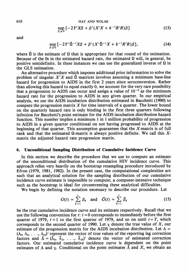
Fig. 2 presents the results for k112 = 3000 and the second-difference restrictions on our cumulative incidence curve estimates for the short and long samples using the empirical process confidence bound paths. The second-difference restrictions allow substantially more curvature (some of which may be excessive) in the estimate of G(t). This is reflected in the slightly larger confidence bound paths and the greater number of elements of f, which are near 0 relative to Fig. 1. The end point confidence bound paths for these second-difference results are similar in shape,


1400000

1300000,

1200000

1100000

1000000,

900000,

800000,

700000/

600000 X

500000

400000 ' -

300000/

200000/

79 80 81 82 83 84 85 86 87 88 89 90 91

PERIOD

Fig. 2. Second-difference restrictions, 95%/ confidence paths constructed using empirical process bounds, k = 9.0 x 106: ?-------, short sample; , complete sample


but slightly wider at t = T corresponding to the second quarter of 1990, relative to those given in Fig. 1. Fig. 3 presents a comparison of the pointwise confidence bound paths and the end point confidence bound paths for the long sample results and smoothness prior and value of k used to construct Fig. 2. Fig. 3 illustrates the excessive optimism implied by constructing confidence paths in this manner, even for the case of tighter 900o confidence interval paths.

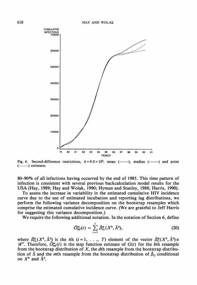
The sampling distributions for the long sample (from the first quarter of 1979 to the second quarter of 1990) cumulative incidence curve estimation results for the USA given in Figs 1 and 2 each yield mean cumulative HIV infections through mid-1990 of approximately 670000. The differences between the mean, median and point estimates of G(t) are very small for all except the last few years, and even then the divergence is not excessive. Fig. 4 presents these three sample paths for second-difference smoothness priors and k112 = 3000. Similar results hold for first- difference smoothness priors. These results imply that, according to the bootstrap unconditional sampling distribution of G(t), our estimation procedure yields very close to an unbiased estimate of G(t) for a wide range of values for k.

The long sample backcalculation estimation paths imply a median infection time for the USA (the time until 50% of all infections occurred) of mid-1983, with


1000000-

900000

800000/

700000-

600000-

500000-

400000-

300000

200000

100000 We2 ....

8. ...

.4. ................

79 80 81 82 83 84 85 86 87 88 89 90 91 PERIOD

Fig. 3. Second-difference restrictions, 900/ confidence paths constructed pointwise and using the end point region, k= 9.0 x 106: ---------, pointwise path; , end point path

618 HAY AND WOLAK


700000-

600000 - -

500000

400000/

300000-

200000 /z

100000

0 ........ ....

79 80 8 1 82 83 84 85 86 87 88 89 90 9 PERIOD

Fig. 4. Second-difference restrictions, k= 9.0 x 106: mean (- ), median (--------) and point ( ) estimates

80-90Wo of all infections having occurred by the end of 1985. This time pattern of infection is consistent with several previous backcalculation model results for the USA (Hay, 1989; Hay and Wolak, 1990; Hyman and Stanley, 1988; Harris, 1990).

To assess the increase in variability in the estimated cumulative HIV incidence curve due to the use of estimated incubation and reporting lag distributions, we perform the following variance decomposition on the bootstrap resamples which comprise the estimated cumulative incidence curve. (We are grateful to Jeff Harris for suggesting this variance decomposition.)

We require the following additional notation. In the notation of Section 6, define

Gmd(t) = E -m (Xb, Ad), (20) i=l

where j(Xb, Ad) is the ith (i = 1, . . ., T) element of the vector m(Xb, Ad)e pT. Therefore, Gbd(t) is the step function estimate of G(t) for the bth resample

from the bootstrap distribution of X, the dth resample from the bootstrap distribution of A and the mth resample from the bootstrap distribution of PG conditional on Xb and Ad.


Following the two-way analysis-of-variance (ANOVA) framework, define the total sum of squared deviations of G61(t) around the mean

B D M

G(t) G

BDMZ Z Z G bd(t) as b=1 d=1 m=1

as B D M

SST(t) = >E E E {Gbmd(t) - G(t)}2. (21) b=1 d-I m=1

Define the 'between' Xb resamples sum of squared residuals as B

SSX(t) = DMZ {Gb(t) - G(t)}2, (22) b-I

where D M

G() D d=I m = tl d=1 m=1

The between Ad resamples sum of squared residuals is defined as D

SSA(t) = BM>j {Gd(t) - G(t)}2, (23) d=1

where B M

&t)MB Yi = i bd m = b=1 m=1

The 'within' Xb and Ab resamples sum of squared residuals is B D M

SS, (t) = j E E {GIbd(t) - Gb (t) - Gd (t) + G(t)}2* (24) b=1 d=1 m=1

Recall that SST(t) = SS,(t) + SSX(t) + SSA(t) for t =1, 2, .. ., T. The quantity SSx(t) measures the amount of SST(t) that is due to variability in X, SSA(t) the amount due to A and SS, (t) is the amount due to variability in the estimate of G(t) conditional on X and A.

In Table 4 we present the values of SST(t), SSx(t)/SST(t), SSA(t)/SST(t) and SSO (t)/SST(t) for four points along the cumulative incidence curve (t = 12, 23, 35, 46) and for two values of k for each type of smoothness prior for the long sample estimation results. Table 5 presents the same two quantities for t = 12, 23, 35 and both smoothness priors for the same values of k for the short sample results. For both sets of results SST(t) is normalized by 1012. All results in Tables 4 and 5 are for B=50, D=50 and M= 10.

Several conclusions emerge from Tables 4 and 5. First the uncertainty in X and A explains most of the variability in G-M (t) for all except the most recent time periods. The ratio SSx(t)/SST(t) far exceeds 0.5 for small values of t and grows larger for intermediate values of t. After values of t near the midpoint of the sample period this ratio slowly begins to decline until it falls very rapidly at the end of

620 HAY AND WOLAK

TABLE 4 Two-way ANOVA for the estimated cumulative incidence curve (complete sample estimates)

Time (t) Smoothness (k) Difference SST(t)t SSx(t)/SST(t) SSA(t)/SST(t) SS(t)/SST(t)

12 1.0 x 108 First 2.8029 0.7955 0.0004 0.2041 23 1.0 x 108 First 1.8038 0.9389 0.0012 0.0600 35 1.0 x 108 First 28.0644 0.8978 0.0038 0.0983 46 1.0 x 108 First 162.0879 0.2804 0.0093 0.7103 12 1.0x 107 First 2.1791 0.9376 0.0002 0.0622 23 1.0 x 107 First 15.3328 0.9806 0.0007 0.0187 35 1.0x 107 First 32.1788 0.9336 0.0033 0.0631 46 1.0 x 107 First 73.8765 0.6568 0.0064 0.3368 12 9.0x 106 Second 1.5702 0.8283 0.0004 0.1713 23 9.0x 106 Second 17.4118 0.9612 0.0009 0.0379 35 9.0 x 106 Second 27.5889 0.9281 0.0033 0.0686 46 9.0x 106 Second 333.0727 0.1037 0.0057 0.8906 12 3.0 x 106 Second 1.7493 0.9182 0.0003 0.0815 23 3.0 x 106 Second 17.3052 0.9759 0.0008 0.0233 35 3.0 x 106 Second 28.5841 0.9368 0.0030 0.0602 46 3.0 x 106 Second 61.4252 0.3946 0.0034 0.6020

tAll numbers in this column have been divided by 1012.

TABLE 5 Two-way ANOVA for the estimated cumulative incidence curve (short sample estimates)

Time (t) Smoothness (k) Difference SST(t)t SSx(t)/SST(t) SSA(t)/SST(t) SS(t)/SST(t)

12 1.0 x 108 First 3.2992 0.8264 0.0002 0.1734 23 1.0 x 108 First 19.5738 0.9128 0.0007 0.0864 35 1.0 x 108 First 239.8909 0.3238 0.0027 0.6735 12 1.0x 107 First 2.3125 0.9386 0.0001 0.0613 23 1.0 x 107 First 18.7249 0.9762 0.0006 0.0232 35 1.0 x 107 First 85.2177 0.6557 0.0026 0.3417 12 9.0x 106 Second 1.9609 0.8540 0.0003 0.1457 23 9.0 x 106 Second 19.4410 0.9062 0.0006 0.0932 35 9.0x 106 Second 812.5445 0.1536 0.0029 0.8435 12 3.0 x 106 Second 1.9027 0.9109 0.0002 0.0889 23 3.0 x 106 Second 21.5210 0.9570 0.0005 0.0425 35 3.0 x 106 Second 432.2561 0.2090 0.0032 0.7878

tAll numbers in this column have been divided by 1012.

the sample period. The ratio SSA(t)/SST(t), as intuition suggests, increases mono- tonically in t for fixed k. Second, the total variability in Gm (t) for t =35 in the short sample results is substantially larger than the corresponding magnitude for t = 46 for the long sample results for all values of k and types of smoothness prior. Third, for all except the case k = 9.0 x 106 and second-difference smoothness priors for both the short and the long sample results, variability in X and A accounts for at least 20Wo of the total variability in Gbd(t) for all t. Even for this selection of smoothing priors and smoothing parameter, for all except the most recent values of t, the fraction of SST(t) accounted for by SSx(t) is above 90Wo, implying that failing to account for the use of both estimated incubation and reporting lag


distributions in the cumulative incidence curve estimation process can substantially underestimate its variability.

A final initially surprising aspect of Tables 4 and 5 is the relatively small amount of the total variability in G-1 (t) which is accounted for by variability in Ad. There are three reasons for this. First, on the basis of the bootstrap approximation to its sampling distribution, A is very precisely estimated. Second, with the exception of A0, the estimated Ai are above 0.5, which does not imply very large inflation factors for the most recent incomplete AIDS diagnosis data, which in turn does not imply the introduction of very substantial errors into the reporting lag correction process. Finally, because our estimation procedure explicitly accounts for the use of reporting-lag-corrected diagnosis data, the effects of the more recent diagnosis totals on the estimate of f3 will be appropriately downweighted.

8. Using Estimation Results to Project Future Cases of Acquired Immune Deficiency Syndrome

Given our estimated cumulative incidence curve and an estimate of the incubation distribution we can project future AIDS cases by running our backcalculation model forwards in time. Because we have the sampling distribution for both the cumulative incidence curve and the AIDS incubation distribution we can apply a bootstrap technique to compute confidence intervals for these point estimates.

Our point estimate of the total number of new diagnoses for period T+ J is

YT+J = XT+JBT+J (25) where XT+J and BT+J are (T+ J)-dimensional vectors defined as follows:

XT+J = (X(T+J)(T+J), X(T+J)(T+J-1), X(T+J)2, X(T+J)1) (26)

BT+J = (1T+J, . . . lT+1, 3Y). (27) The progression probabilities xi are computed from the AIDS incubation distribution as described in Section 2. The parameters (13T+J, . . . 13T+ 1) are the assumed number of new seroconversions for quarters T+ 1 to T+ J. If we wish to incorporate our uncertainty about the values of these elements of BT+J, then we can assume that these parameters are drawn from a known multivariate distribution with this mean vector. For our sample, the parameter vector f E _WT gives our estimate of the total number of new seroconversions for each quarter from the first quarter of 1979 to the second quarter of 1990, for a total of T= 46 quarters.

To compute an estimate of the sampling distribution for our point estimate of AIDS diagnoses for period T+ J, we apply a bootstrap procedure to our equation for YT+J. For each resample m, we draw an XT+j(m) from the bootstrap distribution of XT+J, a O3m from the bootstrap distribution of jl and, if desired, a (fMT+J, . .*m+)' from the assumed prior distribution for the vector of future quarterly

seroconversion totals. Using these three resampled values we compute

Y +J = XT+J(m)'BT+J (28) Repeating this procedure M times yields a bootstrap estimate of the sampling distribution of YT+J from which we can compute confidence intervals. To compute estimates of future AIDS diagnosis totals for all values between T+ J and T+ 1,

622 HAY AND WOLAK

we construct a matrix version of equation (25) which involves BT+J. Computing the sampling distribution of this vector of future diagnosis totals proceeds in the same way. We can then apply the procedures discussed in Section 6 to compute confidence interval paths for this time series of future diagnosis totals.

9. Conclusions and Directions for Future Research We now review several caveats to our results discussed throughout the paper and

then discuss some possible directions for future research. First, as mentioned in Section 2, there is some unknown fraction of AIDS

diagnoses that are never reported. It is unclear how to adjust our totals and associated confidence bound paths for these permanently unreported AIDS cases. Further research is needed to understand the magnitude and variability of this source of underreporting.

A second caveat is our use of a smoothing prior, or roughness penalty, on the estimated cumulative incidence curve for HIV. As mentioned in the discussion of our results, the point estimates of G(t) for both the short sample and the long sample are unaffected by changes in k, for a very wide range of values. However, the 95% confidence paths did vary with k. For the most recent quarters, because of the form of the AIDS incubation distribution, the only hope for obtaining a useful confidence bound on G(t) is to impose a priori restrictions on the form of G(t). One choice is to impose a specific functional form for G(t); our choice was simply to require the function to conform to our intuition that it be smooth. As we have demonstrated, imposing what appears to be a mild roughness penalty on G(t) yields fairly tight confidence bounds. The larger the roughness penalty we are willing to impose the tighter these bounds can become. Nevertheless, to make useful confidence interval statements for the most recent quarters, some smoothness priors or functional form restrictions must be imposed. If we are not willing to make these kinds of assumption very little can be said about the variability in the cumulative incidence curve for HIV for the recent past.

Our procedure can be extended in several directions. The major cost of this undertaking is computational expense. Because of the linear model formulation, the backcalculation procedure that we have presented can be reformulated to take into account covariates in both the incubation distribution and the reporting lag distribution, as long as the covariates are discrete and take on a finite number of values. In this case, a separate model of the form given in equation (3) is estimated for each of the values of the covariate vector. The resulting 13-vectors for each possible value of the covariate vector can then be aggregated to create an estimated population cumulative incidence curve. We hope to undertake this analysis, as more research is produced incorporating covariates into both the incubation distribution and the estimation process for the reporting lag distribution.

Acknowledgements This research was supported, in part, by National Center for Health Services

Research grant HS-06092 to the Hoover Institution. It was begun while Hay was a Senior Research Fellow and Wolak a National Fellow of the Hoover Institution. We are grateful to Peter Bacchetti for providing an estimate of the AIDS incubation


distribution necessary for our empirical analysis. We acknowledge the helpful comments on a previous version provided by Fred Hellinger, Meade Morgan and Dennis Osmond. Jeff Harris deserves special mention for his many useful suggestions. Miriam Culjak, Dana Goldman and Paul Liu provided outstanding research assistance. Two referees provided thoughtful suggestions for a revision of a previous draft.

References Bacchetti, P. (1990) Estimating the incubation period of AIDS by comparing population infection and

diagnosis patterns. J. Am. Statist. Ass., 85, 1002-1008. Bacchetti, P. and Moss, A. (1989) Incubation period of AIDS in San Francisco. Nature, 338, 251-253. Bazaraa, M. S. and Shetty, C. M. (1979) Nonlinear Programming: Theory and Algorithms. New York:

Wiley. Becker, N. G., Watson, L. F. and Carlin, J. B. (1991) A method of nonparametric back-projection

and its application to AIDS data. Statist. Med., 10, 1527-1542. Bickel, P. J. and Freedman, D. A. (1981) Some asymptotic theory for the bootstrap. Ann. Statist.,

9, 1196-1217. Brookmeyer, R. (1991) Reconstruction and future trends in the AIDS epidemic in the U.S. Science,

253, 37-42. Brookmeyer, R. and Damiano, A. (1989) Statistical methods for short-term projections of AIDS

incidence. Statist. Med., 8, 23-34. Brookmeyer, R. and Gail, M. H. (1988) A method for obtaining short-term projections and lower

bounds on the size of the AIDS epidemic. J. Am. Statist. Ass., 83, 301-308. Brookmeyer, R. and Goedert, J. (1989) Censoring in an epidemic with an application to hemophilia-

associated AIDS. Biometrics, 45, 325-335. Brookmeyer, R. and Liao, J. (1990) The analysis of delays in disease reporting: methods and results

for the acquired immunodeficiency syndrome. Am. J. Epidem., 3, 296-306. Carroll, R. J., Wu, C. J. and Ruppert, D. (1988) The effect of estimating weights in weighted least

squares. J. Am. Statist. Ass., 83, 1045-1054. Centers for Disease Control (1990) HIV prevalence estimates and AIDS case projections for the United

States: report based on a workshop. Morb. Mort. Wkly Rep., 39, no. RR-16. (1991) HIV/AIDS Public Information Data Set. Atlanta: Centers for Disease Control. (1993) HIV/AIDS Surveillance Report, pp. 1-23. Atlanta: Centers for Disease Control.

Efron, B. (1979) Bootstrap methods: another look at the jackknife. Ann. Statist., 7, 1-26. (1981) Nonparametric standard errors and confidence intervals (with discussion). Can. J.

Statist., 9, 139-172. (1982) The Jackknife, the Bootstrap, and Other Resampling Plans. Philadelphia: Society for

Industrial and Applied Mathematics. Gail, M. H., Rosenberg, P. S. and Goedert, J. J. (1990) Therapy may explain recent deficits in AIDS

incidence. J. AIDS, 3, 296-306. Harris, J. E. (1990) Reporting delays and the incidence of AIDS. J. Am. Statist. Ass., 85, 915-924. Hay, J. (1989) Projecting the medical costs of HIV/AIDS. In New Perspectives on HIV-related Illness:

Progress in Health Services Research (ed. W. Levee), pp. 84-97. Rockville: National Center for Health Services Research.

Hay, J., Osmond, D. H. and Wolak, F. A. (1991) Projecting the costs of AIDS and ARC in the United States. Final Report to Agency for Health Care Policy and Research, Grant HS-06092. US Depart- ment of Health and Human Services, Public Health Service, Rockville.

Hay, J. and Wolak, F. A. (1990) Bootstrapping HIV/AIDS projection models: backcalculation with linear inequality-constrained regression. Hoover Institution Domestic Studies Working Paper. Hoover Institution, Stanford.

Hessol, N., Lifson, A., O'Malley, P., Doll, L. S., Jaffe, H. W. and Rutherford, G. W. (1989) Prevalence, incidence and progression of Human Immunodeficiency Virus infection in homosexual and bisexual men in Hepatitis Vaccine Trials, 1978-1988. Am. J. Epidem., 130, 1167-1175.

Hyman, J. M. and Stanley, E. A. (1988) Using mathematical models to understand the AIDS epidemic. Math. Biosci., 90, 415-473.

624 HAY AND WOLAK

Liew, C. K. (1976) Inequality-constrained least-squares estimation. J. Am. Statist. Ass., 71, 746-751. Medley, G. F., Zunzunegui, V., Bueno, R. and Lopez Gai, D. (1991) The use of AIDS surveillance

data for short-term prediction of AIDS cases in Madrid, Spain. Eur. J. Epidem., 7, 349-357. Munioz, A., Wang, M.-C., Bass, S., Taylor, J. M. G., Kingsley, L. A., Chmiel, J. S. and Polk, F.

(1989) Acquired Immunodeficiency Syndrome (AIDS)-free time after Human Immunodeficiency Virus Type 1 (HIV-1) seroconversion in homosexual men. Am. J. Epidem., 130, 530-539.

Rosenberg, P. S. (1990) A simple correction of AIDS surveillance data for reporting delays. J. Acq. Immune Def. Synd., 3, 49-54.

Rosenberg, P. S. and Gail, M. H. (1990) Uncertainty in estimates of HIV prevalence derived by backcalculation. Ann. Epidem., 1, 105-115.

(1991) Backcalculation of flexible linear models of the human immunodeficiency virus infection curve. Appl. Statist., 40, 269-282.

Rosenblum, L., Buehler, J. W., Morgan, M. W., Costa, S., Hidalgo, J., Holmes, R., Lieb, L., Shields, A. and Whyte, B. M. (1992) The completeness of AIDS case reporting 1988: a multivariate collaborative surveillance project. Am. J. Publ. Hlth, 82, 1495-1499.

Taylor, J. M. G., Kuo, J.-M. and Detels, R. (1991) Is the incubation period of AIDS lengthening? J. Acq. Immune Def. Synd., 4, 69-75.

Theil, H. and Goldberger, A. S. (1961) On pure and mixed statistical estimation in economics. Int. Econ. Rev., 2, 65-78.

Zeger, S. L., See, L.-C. and Diggle, P. J. (1989) Statistical methods for monitoring the AIDS epidemic. Statist. Med., 8, 3-21.

a procedure for estimating the unconditional … · appl statist. (1994) 43, no. 4, pp. 599-624 a...

Documents