a programmers guide to zpl - university of...
TRANSCRIPT

ZPL Programming Guide
i
A Programmers Guideto ZPL
Lawrence SnyderDepartment of Computer Science and Engineering
University of WashingtonSeattle WA 98195
Version 6.3January 6, 1999
© 1994, 1995, 1996, 1997, 1998 Lawrence Snyder. All rights reserved.

ZPL Programming Guide
ii
ZPL Home Page
Check the ZPL home pagehttp://www.cs.washington.edu/research/zpl/
for access to a compiler, libraries andcomplete information about ZPL

ZPL Programming Guide
iii
Preface
This guide seeks to be a complete introduction to the ZPL programminglanguage and the programming style that it introduces. The presentationassumes the reader is experienced with some imperative programminglanguage such as C, Fortran, Pascal, Ada or the like. Though precise and inmost instances thorough, the guide does not attempt to be a reference manualfor ZPL. Rather, it illustrates typical ZPL usage and explains in an intuitiveway how the constructs work. Emphasis is placed on teaching the reader to bea ZPL programmer. Scientific computations are used as examplesthroughout.

ZPL Programming Guide
i v
Acknowledgments
ZPL is the product of many people's ideas and hard work. It is a pleasure tothank Calvin Lin with whom the initial structure of the language wasdesigned. Calvin has led a committed and enthusiastic team ofimplementors of the prototype ZPL system: Brad Chamberlain, Sung-EunChoi, E Chris Lewis, Jason Secosky and Derrick Weathersby, withcontributions at the early stages from Ruth Anderson, George Forman andKurt Partridge. These dedicated computer scientists have devoted theirminds and hearts to the realization of ZPL's goals. It is a pleasure toacknowledge their creativity: they have given life to ZPL. Others have offeredthoughtful input and comment on the language, including A. J. Bernheim,Jan Cuny, Marios Dikaiakos, John G. Lewis, Ton Ngo, and Peter Van Vleet.
This document has undergone numerous revisions, and many people havecontributed suggestions for its improvement. Thanks are due to GeorgeTurkiyahh for his input on the N-body computation, Sung-Eun Choi for hercomments on median finding and her contributions with Melanie Fulghamto random numbers, Victor Moore for suggesting vector quantization, MartinTompa for assisting with global alignment, and Brad Chamberlain for hisinput on the presentation of advanced topics. E Lewis and Sung-Eun Choipointed out numerous improvements to the programs and text.
The ZPL research has been supported in part by Office of Naval Researchgrant N00014-89-J-1368, the Defense Advanced Research Projects Agencyunder grants N00014-92-J-1824 and E30602-97-1-0152, and the National ScienceFoundation grant CCR 97-10284. Assistance with computer equipment hasbeen received from the National Science Foundation grant CDA-9123308 andDigital Equipment Corporation.

ZPL Programming Guide
v
Dedicated to the memory ofA. Nico Habermann
and the many delightful hours spentdiscussing programming language design
and compiler construction.

ZPL Programming Guide
v i
Contents
Preface............................................................................................................................. iii
Acknowledgments....................................................................................................... i v
Contents......................................................................................................................... v i
Chapter 1Introduction.................................................................................................................. 1
What is ZPL ?.................................................................................................... 1Preliminary ZPL Concepts ............................................................................. 3A Quick Tour of the Jacobi Program............................................................ 5Learning ZPL from this Guide...................................................................... 8Acquiring ZPL Programming Technique.................................................. 9
Chapter 2Standard Constructs .................................................................................................... 12
Data Types.......................................................................................................... 12Operators............................................................................................................ 13ANSI C Object Code......................................................................................... 15Identifiers........................................................................................................... 15Assignment....................................................................................................... 16Control-flow Statements................................................................................ 16
Chapter 3Basic ZPL Array Concepts........................................................................................... 19
Regions............................................................................................................... 19Region Declarations ............................................................................ 21Array Declarations............................................................................... 21Region Specifiers.................................................................................. 22
Directions........................................................................................................... 24Direction Declarations ........................................................................ 24Using Directions with "of" ................................................................ 25Using Directions with "@" ................................................................ 26Comparison of "of" vs "@" ............................................................... 28Borders ................................................................................................... 28Array and Cartesian Coordinates for Directions........................... 29
Promotion ......................................................................................................... 30Index1, Index2, ... .............................................................................................. 31Reduce and Scan .............................................................................................. 34
Chapter 4Program Structure and Examples............................................................................. 37

ZPL Programming Guide
vii
ZPL Programs.................................................................................................... 37Basic I/O............................................................................................................. 39
Text I/O .................................................................................................. 39Binary I/O.............................................................................................. 41
Example Computations.................................................................................. 42Sample Statistics................................................................................... 42Correlation Coefficient ....................................................................... 43Histogram.............................................................................................. 45Uniform Convolution........................................................................ 48
Shift-and-Add Solution.......................................................... 48Scan Solution............................................................................ 49
Counting Connected Components .................................................. 51
Chapter 5Generalizing ZPL ......................................................................................................... 55
Additional Region Specifications................................................................. 55Degenerate Ranges............................................................................... 55@ Compositions................................................................................... 56"At" in Region Specifiers................................................................... 56"Of" Compositions .............................................................................. 56"In" Regions.......................................................................................... 57Combination Specification ................................................................ 57
Dynamic Regions............................................................................................. 58Simplified Region Specification................................................................... 60
Inheritance ............................................................................................ 60Ditto ........................................................................................................ 60
Indexed Arrays.................................................................................................. 61Type Declarations............................................................................................. 63Flooding............................................................................................................. 65Reduction/Scan Revisited............................................................................. 67Region Conformance...................................................................................... 69Procedures ......................................................................................................... 70
Procedure Declarations....................................................................... 70Procedure Prototypes........................................................................... 73Procedure Call....................................................................................... 74Promotion ............................................................................................. 74Recursion............................................................................................... 75
Shattered Control-flow................................................................................... 75Masks.................................................................................................................. 77
Chapter 6Programming Techniques ......................................................................................... 80
Matrix Multiplication ..................................................................................... 80Sparse Matrix Product..................................................................................... 87Ranking.............................................................................................................. 90Histogramming, Revisited ............................................................................ 91

ZPL Programming Guide
viii
Vector Quantization Data Compression..................................................... 93Odd/Even Transposition Sort....................................................................... 95
Chapter 7Advanced ZPL Concepts............................................................................................. 98
Strided Regions and Arrays........................................................................... 98Multidirections................................................................................................. 102Multiregions and Arrays................................................................................ 104Permutations, Gather and Scatter ................................................................ 107
Chapter 8WYSIWYG Parallel Execution.................................................................................. 111
Parallel Machine Model ................................................................................. 111Parallel Execution of ZPL ............................................................................... 113
Memory Allocation............................................................................. 113Processor Code...................................................................................... 114
Estimating Program Performance................................................................ 115"@" References..................................................................................... 116Strided Regions .................................................................................... 116Reductions/Scans ................................................................................ 117Flooding................................................................................................. 117Scalar computations............................................................................ 118Permutations ........................................................................................ 118I/O ........................................................................................................... 119Summary on Estimation.................................................................... 119
Closing Remarks on Performance ............................................................... 119
Chapter 9Computational Techniques....................................................................................... 121
Sequential Computation................................................................................ 121Inconsequential Code Fragments..................................................... 122Sequential Routines for Promotion ................................................ 124
N-Body Computations.................................................................................... 128Single Particle Pushing....................................................................... 130Batched Pushing Solution ................................................................. 132
Thinking Globally -- Median Finding......................................................... 134Random Number Generation ...................................................................... 136
Chapter 10ZPL and Future Parallel Programming................................................................... 140
ZPL Reference............................................................................................................... 141
AppendixFundamental Constants, Standard Functions and Timers ................................ 142
Fundamental Constants................................................................................. 142

ZPL Programming Guide
ix
Scientific Functions......................................................................................... 142Timers ................................................................................................................ 143
Index ............................................................................................................................... 145

ZPL Programming Guide
x

ZPL Programming Guide
1
-- Chapter 1 --
Introduction
ZPL is a new programming language that is especially effective for scientificand engineering computations. It is intended to replace languages such asFortran and C for technical computing. The programming advantages of ZPLwill become evident as its features are explained in subsequent chapters. Inthis chapter ZPL is illustrated to give the curious a quick overview, and toprepare the student for the more thorough presentation to follow.
What is ZPL ?
ZPL* is a programming language suitable for scientific and engineeringcomputations. It can be described in other ways as well:
• ZPL is an array language. Expressions such as X + Y have been generalizedto apply to whole arrays as well as simple scalars, depending on how X andY are declared. The language has standard programming constructs, such asif statements and procedures. These concepts have their normal meaning,though there is often an array generalization. Expressions involving arraysare convenient and natural to write, especially for scientists and engineers.Not only does an array language save the programmer from writing manytedious loops and specifying error prone index calculations, it enables thecompiler to identify parallelism that will speed the computation.
• ZPL is a machine independent programming language, meaning that ZPLprograms run well on both sequential and parallel computers.Programmers need not concern themselves with machine specifics.Machine independence is an essential requirement for programs that willbe shared among many researchers with different computers. It is probablymost important for programs used over a long period of time, since theyare simply recompiled when an old machine is replaced by a new one.Details of ZPL's most important machine independence feature, the what-you-see-is-what-you-get (WYSIWYG) performance capability, are presentedin Chapter 8.
• ZPL is an implicitly parallel programming language. That is, although ZPLwas designed to simplify programming parallel computers, programmers
* ZPL is mnemonic for the phrase "Z-level Programming Language," a reference to a componentof the programming model that it implements [Alverson et al., 98].

ZPL Programming Guide
2
do not specify how the computation is performed concurrently. Nor dothey insert interprocessor communication. The ZPL compiler isresponsible for producing parallel object code from the source program, andfor taking care of all details necessary to exploit the target parallel computer.There are times when the programmer will want to consider how thecomputation is performed in parallel, e. g. when deciding amongalternative ways of implementing a computation. But generally,programmers are only concerned with expressing the computation toproduce the right result.
Perhaps the most important property of ZPL for scientific programmers is thatit can be compiled to run fast on parallel computers. For example, the Jacobiiteration, which will be used as an example throughout the remainder of thischapter, has been reported to have the performance approximating C, asillustrated in Figure 1.1 [Lin & Snyder 94]. In the experiment the program(illustrated in Figure 1.2) was compiled, and then run on the Kendall SquareResearch KSR-2, a "shared memory" parallel computer, and the IntelCorporation Paragon, a distributed memory or "message passing" parallelcomputer. The two machines are representative of the principal classes ofcommercially available parallel computers. The program was executed untilconvergence (929 iterations). Its performance was compared with a Cprogram handcoded for each machine.
4
8
12
16
4 8 12 16
spee
dup
processors
Jacobi Speedup on the Intel Paragon
linearhand coded
zpl
4
8
12
16
4 8 12 16processors
Jacobi Speedup on the KSR-2
linearzpl
hand coded
Figure 1.1. Speedup with respect to the handcoded C programfor the Jacobi program executed on the Intel Paragon and theKSR-2.

ZPL Programming Guide
3
The Jacobi computation is a simple program, and good performance is to beexpected. Comparable results for other, more substantial computations havealso been reported [Lin et al. 95, Ngo et al. 97].
Preliminary ZPL Concepts
Most ZPL concepts are intuitive and easy to understand by scientists andengineers familiar with other programming languages, e.g. Fortran or C. Tointroduce these concepts, consider the Jacobi iteration as an example thatillustrates representative usage.
Jacobi: Given an array A, iteratively replace its elements with the averageof their four nearest neighbors, until the largest change between twoconsecutive iterations is less than delta .
For the example, the array A will be an n × n two dimensional array initializedto zero, except for the southern boundary, which is set to the constant 1.0 in
1 program Jacobi; 2 /* Jacobi Iteration 3 Written by L. Snyder, May 1994 */ 4 config var n : integer = 512; -- Declarations 5 delta : float = 0.000001; 6 7 region R = [1..n, 1..n]; 8 var A, Temp: [R] float; 9 err : float;1011 direction north = [-1, 0];12 east = [ 0, 1];13 west = [ 0,-1];14 south = [ 1, 0];1516 procedure Jacobi();17 begin18 [R] A := 0.0; -- Initialization19 [north of R] A := 0.0;20 [east of R] A := 0.0;21 [west of R] A := 0.0;22 [south of R] A := 1.0;2324 [R] repeat -- Body25 Temp := (A@north + A@east26 + A@west + A@south)/4.0;27 err := max<< abs(A - Temp);28 A := Temp;29 until err < delta;30 end;
Figure 1.2. ZPL program for the Jacobi computation.

ZPL Programming Guide
4
each position. The tolerance delta will be 0.000001 . The ZPL Jacobiprogram is shown in Figure 1.2.
Several features of the language are evident, even without any explanation ofhow the program works.
Like most languages, ZPL programs begin with declaration statements. Allvariables in ZPL programs must be declared. The computational part of theprogram has been further subdivided by the programmer into "initialization"and "body" sections. Though this division of activities is not required by thelanguage, it is generally good practice to concentrate initialization into a blockat the start of the program.
There are punctuation characteristics of ZPL that are also evident from theJacobi program.
The assignment symbol in ZPL is := with no space between the twocharacters. Assignment has the same meaning as in other programminglanguages that simply use an equal sign, e.g. Fortran and C. Thus, the valuecomputed on the right-hand side becomes the value of the name indicated onthe left-hand side. The equal sign is also used in ZPL, but it serves two otherroles. First, the = symbol is used to give values to names in cases where thevalues cannot be changed in the program. The declaration section illustratesmultiple uses of = in this form (Lines 7, 11-14). Second, the equal sign is usedwhen testing for equality, as might be required in an if -statement. As asimple intuitive rule, := is used for changing values of variables, while = isused in cases where equality is the intended meaning.
Unlike Fortran, but like C, every statement in ZPL is terminated with asemicolon. This is true even if it appears that some other word orpunctuation character might also serve to indicate statement termination.Since the end-of-line is not a statement terminator, long statements can easilybe written across multiple lines without any continuation symbols, as in thetwo-line assignment to Temp (Lines 25-26).
The one role reserved for end-of-line in ZPL is as a comment terminator.ZPL has two kinds of comments:
Any text between -- and the end of the line is a comment.Any text between /* and the first following */ is a comment.
Thus, the -- symbol is typically used for short comments (Line 18), while a/* */ pair is used for multiline commentary (Lines 2-3).

ZPL Programming Guide
5
A Quick Tour of the Jacobi Program
Though all of the programming constructs will be explained later, a brief"walk through" of the Jacobi program of Figure 1.2 can serve as anintroduction to ZPL and its approach to computation.
A fundamental concept in ZPL is the notion of a region. A region is simply aset of indices. For example, (Line 7),
region R = [1..n, 1..n];
specifies the standard indices of an n × n array, i.e. the set of ordered pairs{(1,1), (1,2), . . ., (n,n)} . Regions can be used to declare arrays of asize corresponding to the index set. Thus, (Line 8),
var A, Temp: [R] float;
declares two n × n array variables, A and Temp, composed of floating pointnumbers with indices given by region R. The final variable declaration, (Line9),
err: float;
does not mention a region, and so err is declared to be a simple scalarfloating point variable.
The program next declares a set of four directions. Directions are used totransform regions. They are vectors with as many elements as the region hasdimensions. The four 2-dimensional direction declarations, (Lines 11-14),
direction north = [-1, 0];east = [ 0, 1];west = [ 0,-1];south = [ 1, 0];
point unit distance in the four cardinal compass directions. For example,north of any index position will be found by subtracting one from the firstelement of the index pair. Examples of transforming regions with directionsinclude expressions with "of" and "@", illustrated momentarily.
Regions also allow ZPL computations to be extended to operate on entirearrays without explicit looping. By prefixing a statement with a regionspecifier, which is simply the region name in brackets, the operations of thestatement are applied to all elements in the array. Thus, (Line 18),
[R] A := 0.0;

ZPL Programming Guide
6
assigns 0.0 to all n2 elements of array A.
Since many scientific problems have boundary conditions, it is oftennecessary to provide borders to array data structures. In Fortran or C this isaccomplished by increasing the size of an array from, say, n × n to n+2 ×n+2 , but doing so misaligns the indices. In ZPL the region specifier can beused to augment arrays with borders. Extending the array A with borders andinitializing their values is the role of the next four lines, (Lines 19-22),
[north of R] A := 0.0;[east of R] A := 0.0;[west of R] A := 0.0;[south of R] A := 1.0;
The region specifier [ d of R] is an expression that defines a region adjacentto R in the d direction, i.e. above R for the case where d=north . The statementis then applied to the elements of the region. Thus, [north of R] definesthe index set which is a 0th row for A. Since A does not have these indices,the ZPL compiler extends A to have a 0th row. The assignment A := 0.0initializes these elements with 0.0 . The successive effects of the fourinitialization statements are illustrated in Figure 1.3. (The programmercould include the "missing" corner elements simply by using a directionpointing towards the corner, e.g. [northeast of R] .)
A [north of R] A:=0; [east of R] A:=0;
[west of R] A:=0; [south of R] A:=1;
0's
1's
Figure 1.3. Schematic of the creation and initialization of borders of A.
With the declarations and initialization completed, programming thecomputation is simple. The repeat -loop, which iterates until the conditionbecomes true, has three statements:
• Compute a new approximation by averaging all elements (Lines 25-26).

ZPL Programming Guide
7
• Determine the largest amount of change between this and the newiteration (Line 27).
• Update A with the new iteration (Line 28).
Since the repeat statement is prefixed by the [R] region specifier, allstatements in the loop are executed in the context of the R region, i.e. over theindices of R. The statements operate as follows.
The averaging illustrates how explicit array indexing is avoided in ZPL byreferring to adjacent array elements using the @ operator with a direction.The statement, (Lines 25-26),
Temp := (A@north + A@east + A@west + A@south) / 4.0;
finds for each element in A the average of its four nearest neighbors andassigns the result to Temp. An expression A@d, executed in the context of aregion R, results in an array of the same size and shape as R offset in thedirection d, and composed of elements of A. As illustrated in Figure 1.4, A@dcan be thought of as adding d to each index, or equivalently in this case,shifting A.
A A@north A@east A@west A@south
••
••
Figure 1.4. Referencing A modified by @ in the context of a region specifiercovering all of A; the dots shown in A correspond
to element (1,1) in the shifted arrays.
Since the region specifier on the repeat -loop provides the context for allstatements in the loop body, the operations of this statement are applied to allelements of the arrays. The four arrays are combined elementwise, yieldingthe effect of computing for element (i,j) the sum of its four nearest neighbors.This can be seen by the following identities:
(i,j)@north ≡ (i, j) + north ≡ (i, j) + (-1, 0) ≡ (i-1, j)(i,j)@east ≡ (i, j) + east ≡ (i, j) + ( 0, 1) ≡ (i, j+1)(i,j)@west ≡ (i, j) + west ≡ (i, j) + ( 0,-1) ≡ (i, j-1)(i,j)@south ≡ (i, j) + south ≡ (i, j) + ( 1, 0) ≡ (i+1, j)
Each of the n2 sums is then divided by 4.0 and the result is stored into Temp.

ZPL Programming Guide
8
To compute the largest change of any element between the current and thenext iteration, (Line 27), more elementwise array operations are performed.The underlined subexpression,
err := max<< abs(A - Temp) ;
causes the elements of Temp to be subtracted from the corresponding elementsof A, and then the (floating point) absolute value of each element is foundyielding an intermediate array with values abs(A 1,1-Temp 1,1), abs(A 1,2-Temp1,2),..., abs(A n,n-Tempn,n) . This computes the magnitude of changeof all the elements. To find the largest among these, a maximum reduction(max<<) is performed. This operation "reduces" the entire array to its largestelement. The maximum is then assigned to err , a scalar variable, thatcontrols the loop.
The final statement of the loop, (Line 28),
A := Temp;
installs Temp as the updated value of A.
The termination test for the iteration, err < delta , is simply thecomparison of two scalar values, since both are declared as scalars. The deltavariable is a configuration parameter, meaning that it is given a default valuein the declaration at the top of the program. Optionally, the value can bechanged on the command line when the program is executed. Thus, both thesize of the problem (n) and the tolerance, can be changed on successive runswithout recompiling the program.
Learning ZPL from this Guide
It takes some time to learn any programming language. But programmersreport that ZPL is very intuitive and has few idiosyncrasies, so it is regarded aseasy to learn. This guide has been organized to aid in acquiring basicproficiency quickly:
• Chapter 2 describes those ZPL features found in other programminglanguages; most readers with programming experience should be able toread this chapter quickly.
• Chapter 3 explains the most fundamental concepts new to ZPL; nearly all ofthem have been introduced in this chapter.
• Chapter 4 illustrates these concepts with small programming examples.
At the completion of Chapter 4, it should be possible to write and run simpleZPL programs. Although the computations may be trivial, it is advantageous

ZPL Programming Guide
9
to run a program just to become familiar with the mechanics of programcompilation and execution.
• Chapter 5 introduces more powerful concepts, including global operations.• Chapter 6 presents another batch of examples illustrating the new concepts.• Chapter 7 completes the language introduction by presenting advanced
concepts.
At the completion of Chapter 5 more interesting programs can be written andrun, and after Chapter 7, essentially the full power of the language isavailable.
• Chapter 8 explains information programmers will want to know if theyplan to run ZPL programs on parallel computers.
• Chapter 9 describes programming techniques with further examples.
Though these last chapters are optional in terms of getting started with thelanguage, they may be the most important for programmers who want toproduce high quality machine independent programs.
Acquiring ZPL Programming Technique
Like all programming languages, there is a certain technique to writing inZPL. "Technique" refers to the basic programming idioms, the "standard"ways to encode data and operate on it, tricks and other experiential knowledgeprogrammers use when they program. For example, Fortran programmers"know" to traverse an array down the columns, while C programmers"know" to traverse it across the rows, because the arrays are stored in thatorder, respectively, and so locality, and hence performance, are enhanced.Though this knowledge is part of the programming technique for theselanguages, it is not ZPL technique, since traversing an array is rare. In ZPLmanipulating whole arrays is basic, and the compiler performs the traversing.This motivates developing a new programming technique.
When first writing ZPL code, a common pitfall is to rely too literally onknown techniques. Programmers learning ZPL often think of computationsin terms of the primitive scalar operations required in other programminglanguages, rather than the whole array manipulations those primitiveoperations implement. Consequently, when thinking about how to write aZPL program, a common mistake of first-time programmers is to attempt toexpress these primitive scalar operations directly in ZPL. Though it ispossible, it's the compiler's task to produce the primitive scalar code. Theprogrammer's task is to express the high level array manipulations thatdefine the computation.

ZPL Programming Guide
10
For example, many of us know the dense matrix-matrix multiplicationcomputation as a triply nested loop that is frequently shown in Fortran or Cprogramming manuals,
FORTRAN MM C MM
DO 10 J = 1,N for (i=0;i<n;i++){ DO 10 I = 1,N for (j=0;j<n;j++){ DO 10 K = 1,N for (k=0;k<n;k++){
10 C(I,J)=C(I,J)+A(I,K)*B(K,J) c[i][j]=c[i][j] +a[i][k]*b[k][j];
} }}
This code describes one way to compute matrix product using element-at-a-time scalar operations, but it is not the definition of the computation taughtin linear algebra class. There, students are told that Cij is the dot-product ofrow i of A and column j of B. This definition, if interpreted literally, does notlead to a very efficient computation, and so may be considered to be tooabstract. The ZPL solution is intermediate, less abstract than linear algebra,but more abstract than an element-at-a-time approach.
As explained in Chapter 6, the "obvious" ZPL program for matrixmultiplication is
[1..n,1..n] for k := 1 to n do C += (>>[,k] A) * (>>[k,] B);
end;
which replicates the k th column of A and the k th row of B to compute the k th
term of all of the dot-products for C at once. (The necessary concepts areexplained in Chapter 5.) This approach may not be the first matrixmultiplication solution to come to mind, but as ZPL technique is acquired, itis more likely to become natural. The statement has all the characteristics ofgood ZPL technique: It computes over arrays rather than scalars, in this caserows and columns; it uses the powerful flood operator (>>) to be spaceefficient; it is very efficient on parallel computers [van de Geijn & Watts 97];and at three lines is about the shortest solution possible.
The conclusion is that programming in an array language requires a differenttechnique than programming in a scalar language. This book givesnumerous examples and illustrations to help the reader acquire good ZPLtechnique. Perhaps, at the start an array solution will take more thinking, butthe thinking will involve high-level concepts, not the nitty-gritty details ofsubscript expressions. Once one acquires the technique, programming inZPL is natural, and the solutions are likely to be shorter, easier to write,simpler to debug and elegant. An array language is just more convenient.

ZPL Programming Guide
11
References
G. A. Alverson, W. G. Griswold, C. Lin and L. Snyder, 1998, "Abstractions forPortable, Scalable Parallel Programming," IEEE Transactions on Paralleland Distributed Systems, Vol 9, No. 1 (to appear)
Calvin Lin & Lawrence Snyder, 1994, "SIMPLE Performance Results in ZPL,"In K. Pingali, U. Banerjee, D. Gelernter, A. Nicolau and D. Padua (Ed.s),Languages and Compilers for Parallel Computing, Springer-Verlag, pp.361-375.
C. Lin, L. Snyder, R. E. Anderson, B. Chamberlain, S. Choi, G. H. Forman, E. C.Lewis, W. D. Weathersby, 1995, "ZPL vs HPF: A Comparison ofPerformance and Programming Style," Technical Report 95-11-05,University of Washington.
Ton A. Ngo, Lawrence Snyder, Bradford Chamberlain, 1997, "Portableperformance of data parallel languages," Proceedings of SC97: HighPerformance Networking and Computing.
Robert van de Geijn and JerrellWatts, 1997, "SUMMA: Scalable universalmatrix multiplication algorithm," Concurrency Practice andExperience, 9(4):255-274

ZPL Programming Guide
12
-- Chapter 2 --
Standard Constructs
ZPL has many features found in other programming languages. In thischapter those ZPL facilities that are similar to structures in other languagesare briefly described, since they are likely to be familiar to experiencedprogrammers.
Data Types
Variables in ZPL can be declared to be any of the following primitive datatypes. The data sizes are machine dependent, though typical sizes are given.
Value TypesSigned Unsigned
boolean logical data, stored as a bytechar printable character, byte size
sbyte ubyte byte datashortint ushortint half size integerinteger uinteger standard size integer (32 bits)longint ulongint double size integerfloat single precision floating pointdouble double precision f.p. (64 bits)quad quadruple precision* f.p. (128 bits)complex single precision complex numberdcomplex double precision complex numberqcomplex quadruple precision* complex number
The unsigned types corresponding to signed types have one more bit ofprecision, but no negative representation. The complex types are pairs offloating point numbers of the indicated precision representing the real andimaginary parts of a complex number. Two other types, file and string , areprovided, but have applications limited chiefly to I/O. (Chapter 4 treats basicI/O.)
Derived Typesarray d-dimensional array of elements of like typeindexed array d-dimensional array of elements of like typerecord user defined type composed of fields
* Not available on some computers, where it defaults to double .
ZPL Programming Guide
13
"Arrays" are called "parallel arrays" when it is necessary to distinguish themfrom "indexed arrays." The semantic distinction is explained in Chapter 5.
Region Typesregion index set, defining iteration and value spacesdirection tuple of signed integers for defining array offsets
Variations on the region types allow for both multiregions andmultidirections. Unlike other types, the region types are "not first class,"meaning that they cannot be assigned or passed to or from a procedure.
Operators
ZPL has a standard set of operators that partition into the usual groups.
Arithmetic Operators+ addition- subtraction* multiplication/ division^ exponentiation+ plus (unary), i.e. no-op- negation (unary)% modulus, i.e. a%b = a mod b
Relational Operators= equality!= inequality< less than> greater than<= less than or equal to>= greater than or equal to
Logical Operators! logical negation (unary)& logical and| logical or
Additionally, bitwise operations on integers and shifting the bits of an integerare supported through the use of value returning built-in functions,
Bitwise Built-in Functionsbnot(a) bitwise negation of the bits of integer aband(a,b) bitwise and of corresponding bits of integers a, bbor(a,b) bitwise or of corresponding bits of integers a, bbxor(a,b) bitwise exclusive or of corresponding bits of

ZPL Programming Guide
14
integers a, bbsl(s,a) shift bits of integer s left a places, filling with 0'sbsr(s,a) shift bits of integer s right a places, filling with 0's
For the purposes of the logical operators, any zero operand value is taken tobe logical false, and any nonzero operand value is taken to be logical true.Further, in the results of logical expressions, false and true are represented as0 and 1, and have type boolean.
Exponentiation is compiled in a special way. When the exponent is a smallinteger constant, i.e. 2, 3 or 4, the ZPL compiler produces efficient customizedcode based on multiplication. In all other cases, i.e. larger integer constants,floats, etc., the built-in function pow() is invoked. When the exponent is 0.5,it is more efficient to use the built-in function sqrt() .In general the operators have the precedence given in Table 2.1.
+ - ! (unary) Highest precedence, binds most tightly<< || >> ## (reduce, scan, flood, permute)^* / %+ - (binary)< > <= >= = !=& | Lowest precedence, weakest binding
Table 2.1. Precedence of ZPL operators. Notice that reduce, etc.bind more tightly than all binary arithmetic operators.
When a sequence of binary operators of equal precedence is used withoutparentheses, left associativity is assumed, i.e.
a - b - c - d ≡ ((a - b) - c) - d
Operators can generally be used with operands of any type according to thefollowing convention: Given the ordering on base types,
boolean Lowestsbyteubyte, charshortintushortintintegeruintegerlongintulongintfloat complexdouble dcomplexquad qcomplex Highest
ZPL Programming Guide
15
any expression combining two base types produces a result of the higher type,which will be a complex type if either operand is complex.
Conversion to a specific type can be achieved by a function of the form
to_ type()
where the nonitalic characters must be given literally, and type is chosenfrom the numeric types. Thus, to_float(i) converts variable i to itsfloating point equivalent. All conversions follow the rules of C, soconversion of numbers from higher to lower types can have unpredictableresults.
ANSI C Object Code
The ZPL compiler converts ZPL source text to ANSI C object code. Theresulting C program is then compiled for the target computer using thenative C compiler for that computer together with machine specific libraries.These two steps are combined in the invocation of zc under UNIX.Generally, the base data types and operators presented in the last two sectionswill have their semantics determined by the characteristics of C and theimplementing hardware.
Consequences of this process include:
• The size of certain base data types (shortint , ushortint , etc.) isinherited from the native C compiler; quad is available only if supportedby the target C compiler.
• All properties of floating point arithmetic are inherited from the nativeC and hardware implementation, and may not conform to the IEEEstandard.
• The standard scientific functions are derived from the C library math.h .• Scalar C procedures can be used in a ZPL program if prototyped in ZPL
(see Chapter 5) and incorporated into the compilation.
Consult the installation notes for your version of the compiler for furtherinformation.
Identifiers
Identifiers are used to name variables and other constituents of ZPLprograms. In general, an identifier is any combination of lower anduppercase letters including underscore (_) and numerals that does not startwith a numeral. ZPL is case sensitive, meaning that
aaa, aaA, aAa, aAA, Aaa, AaA, AAa, AAA

ZPL Programming Guide
16
are all distinct identifiers. The keywords of the language, e.g. if , for ,integer , etc. are prohibited as identifiers.
As a convention ZPL programmers capitalize the first letter of array variablesand regions as an aid to reading the program. Since most features of thelanguage apply equally to arrays as well as to simple scalar values, signifyingthe arrays with capitals calls attention to them. Since they have characteristicsin the language that scalars do not possess -- they are a source of parallelism,require regions specifiers, etc. -- it is helpful to distinguish them at a glancefrom scalars. This book follows the capitals-for-arrays policy.
Assignment
As described in the introduction, the basic assignment operator is :=, but ZPLhas extended assignment operators in the style of C.
Assignments:= assignment+= plus-equal a += b ≡ a:= a+b
-= minus-equal a -= b ≡ a:= a-b
*= times-equal a *= b ≡ a:= a*b
/= divide-equal a /= b ≡ a:= a/b
%= mod-equal a %= b ≡ a:= a%b
&= and-equal a &= b ≡ a:= a&b
|= or-equal a |= b ≡ a:= a|b
Notice that all assignments are statements, i.e. ZPL has no expressionassignments.
Control-flow Statements
The control-flow of a language describes the order of execution of theprogram's statements. Though ZPL is efficiently executed in parallel, itderives its concurrency by applying operations to arrays, not by theprogrammer specifying statement sequences to execute simultaneously.Thus, except for "shattered control flow" discussed in Chapter 5, ZPLstatements are executed one-at-a-time.
ZPL uses familiar control structures found in sequential languages.

ZPL Programming Guide
17
Control-flow Statementsif lexpression then statements
{else statements} end;
if lexpression then statements {{elsif lexpression then statements}}
{else statements} end;
for var := low to high {by step} do statements end;
for var := high downto low {by step} do statements end;
while lexpression do statements end;
repeat statements until lexpression;
return { expression}; -- from a procedureexit; -- from the innermost loopcontinue; -- to the next loop iterationhalt; -- terminate executionbegin statements end; -- compound statement
The non-italicized text must be given literally. Items in braces {} are optional;items in double braces {{}} may be repeated zero or more times. Italicizeditems must be replaced by program text of the proper type: var is a variable;lexpression is a logical expression; low, high and step are numericalexpressions; statements is any statement sequence where each statement isterminated by a semicolon.
The control-flow statements, though generally self-evident, exhibit somecharacteristics worth noticing. The terminator for statements list is:
Statement list following Terminated bythen else, elsif or end;else end;do end;repeat untilbegin end;
The for -loop iteration variable is increased by step or 1 (if step is not given)when the separator between low and high is to ; it is decreased by step or 1when the separator is downto . Thus, there is no need for negative stepvalues. There is no goto statement in ZPL. Rather, it is possible toselectively execute statements (if ), to iterate (for, while, repeat ), topreempt iteration (exit ), to skip to the next loop iteration (continue ) and toterminate execution (halt ). Statements can be grouped into a compoundstatement using a begin end pair. These control structures are sufficient torealize any sequence of statement executions, and are thought to lead to more

ZPL Programming Guide
18
easily understood and debugged programs compared with programs that relyheavily on goto 's for their control flow.
The principal difference between using else if and using elsif can be seenby noticing the number of end 's required to terminate a cascade of tests:
if ... if ... then ... then ... else if ... elsif ...
then ... then ... else if ... elsif ...
then ... then ... else ... else ...
end; end; end;
end;
That is, each use of if starts a new (nested) statement that must eventually beterminated by an end , while elsif "continues" the if in which it appears.
Finally, since leading blanks and tabs are ignored, indenting is available toimprove the readability of a program. Indenting, commenting and inclusionof white-space is recommended, as it is thought to promote readability.
ZPL Programming Guide
19
-- Chapter 3 --
ZPL Array Concepts
In this chapter basic array constructs of ZPL are explained. Each topic istreated in a separate section. The goal is to provide a sufficiently completeunderstanding of the basic concepts to write simple ZPL programs. (SeeChapter 4.) More advanced concepts are treated in subsequent chapters. Thetopics are:
RegionsRegion DeclarationsArray DeclarationsRegion Specifiers
DirectionsDirection DeclarationsUsing Directions with "of"Using Directions with "@"Comparison of "of" vs "@"BordersArray and Cartesian Coordinates for Directions
PromotionIndex1, Index2, . . .Reduce and Scan
Familiarity with the overall concepts of ZPL, as introduced in the Jacobiprogram walk-through of Chapter 1, is assumed.
Regions
ZPL programmers write few loops in their programs and perform aminimum of index manipulation. This makes ZPL programs shorter,presumably easier to write and read, and with a lowered chance of notationalerrors. More importantly, the compiler is able to produce highly optimizedcode that runs well on sequential as well as parallel computers. The"region" concept is critical to making these advantages possible.
A region is a set of indices of a fixed rank. That is, a rank r region is theCartesian product of r dense integer sequences, the lower and upper limits ofwhich are programmer specified. The lower and upper limits are separated by

ZPL Programming Guide
20
"double dots", these pairs are separated by commas, and the wholespecification is enclosed in brackets. Thus, an example 2×2 region is
[1..2, 1..2] = {(1,1), (1,2), (2,1), (2,2) }
where the pairs in parentheses are the rank 2 indices of the region. Rank rindices have r positions in the index tuples, called dimensions.
The limits are programmer-specified, so they can be 0-origin, as in the 2×2region,
[0..1, 0..1] = {(0,0), (0,1), (1,0), (1,1) }
or they can start and end at any other integral value, including negativevalues. Thus,
[-1..1,-1..1,-1..1] = {(-1,-1,-1), (-1,-1, 0), (-1,-1, 1), (-1, 0,-1), (-1, 0, 0), (-1, 0, 1), (-1, 1,-1), (-1, 1, 0), (-1, 1, 1), ( 0,-1,-1), ( 0,-1, 0), ( 0,-1, 1), ( 0, 0,-1), ( 0, 0, 0), ( 0, 0, 1), ( 0, 1,-1), ( 0, 1, 0), ( 0, 1, 1), ( 1,-1,-1), ( 1,-1, 0), ( 1,-1, 1), ( 1, 0,-1), ( 1, 0, 0), ( 1, 0, 1), ( 1, 1,-1), ( 1, 1, 0), ( 1, 1, 1)}
is a region of the 27 lattice points adjacent to the origin in three space,including the origin, and
[-10..10] = {(-10), (-9), (-8), (-7), (-6), ( -5), (-4), (-3), (-2), (-1), ( 0), ( 1), ( 2), ( 3), ( 4), ( 5), ( 6), ( 7), ( 8), ( 9), (10)}
is a one dimensional array with indices spanning the interval from -10 to 10 .
The general form of a region specification in ZPL is
[ l1..u1, l2..u2, . . ., lr..ur]
wherel1, u1, l2, u2,..., lr, ur are required to be integers, possibly signed, given asexplicit constants, declared constants or configuration variables (see below),such that li ≤ ui. The terminology is:
li is called the lower limit of dimension i.ui is called the upper limit of dimension i.r is called the rank of the region.(ui - li+1) is called the size of the ith dimension.

ZPL Programming Guide
21
Notice the ordering of the dimensions is from left to right, i.e. l1..u1 is theindex range of the first dimension.
The region is the Cartesian product of the integer intervals
[ l1..u1, l2..u2, . . ., lr..ur]= { l1, l1+1, ...,u1 } × { l2, l2+1, ...,u2 } × . . . × { lr, lr+1, ...,ur }
It must be emphasized that a region is simply an index set. It is not an array.
Region DeclarationsSince scientific and engineering computations often perform operationsrepeatedly over a set of indices, it is convenient to give regions names tosimplify their frequent use. The region declaration assigns a name to aregion. For example,
region W = [1..10, 1..n]; -- Declaration of a 10 x n region
defines a two dimensional region W with indices ranging from 1 through 10 inthe first dimension and from 1 through n in the second dimension.
The general form of a region declaration is
region RName = [ l1..u1, l2..u2, . . ., lr..ur];
where RName is a user selected identifier that names the region. See Table3.1 This association remains fixed. As with all identifiers, it is thought to begood style to select meaningful names for regions, though because of theirusage patterns programmers tend to prefer short names. Regions are "notfirst class", and so they cannot be assigned, or passed to or returned fromprocedures. See also dynamic regions in Chapter 5.
Array DeclarationsAs noted above regions are simply sets of indices; they are not arrays.Separate declarations are required to define array variables, with regionsgiving the indices. Specifically, arrays are declared like other variables, exceptthey have a region specified in brackets following the colon. (This is a regionspecifier, as explain next.) For example,
var A, B, C : [R] double;
declares three arrays with the same rank and index set, which is given by R.Though it is typical to declare arrays over regions that have been givennames, it is not necessary. So
var U, V, W : [1..n] ubyte;

ZPL Programming Guide
22
is a legal declaration for three vectors of unsigned bytes, using an explicitregion specification. It is somewhat better style to use named regions todeclare arrays, since presumably the region has a meaning in the problemsolution, e.g. "interior" of problem domain, "odd elements", etc., andassociating the variables with this meaning is generally clarifying. But the
Region Declaration Exampleslower upperlimit, limit, size,
Example rank dim 1 dim 1 dim 1region V=[-10..10]; 1 -10 10 21region Board=[1..8,1..8]; 2 1 8 8region Rubix=[1..4,1..4,1..4]; 3 1 4 4region Symmetric=[-10..10,-n..n]; 2 -10 10 21
Table 3.1. Examples of region declarations
main advantage to using named regions in array declarations is that thearrays can have borders "automatically allocated" as described below.
Region SpecifiersRegion specifiers are region names or region expressions in square brackets,e.g. [V] . Though region specifiers are used for declaring arrays as justexplained, their most common use is as prefixes to statements. Whenprefixing a statement, a region specifier of rank r asserts that all operations onrank r arrays in the statement are to be performed for the indices specified bythe region. For example, assuming X, Y and Z are arrays with the same rankas the region V, the statement
[V] X := Y + Z;
specifies that the elements of Y having indices in V are to be added to thecorresponding elements in Z, i.e. those with the same indices, and the resultsof these sums are to be stored in the corresponding elements of X. X, Y and Zmust be declared to have at least the indices of V, though they can have otherindices as well. Any elements of X with indices not in V are unchanged bythe assignment.
For example, the declarations
region V = [1..5];Vpre = [1..3];
var X, Y, Z : [V] integer;
define two regions and establish X, Y and Z as five element arrays withindices given by V. Assuming initial values
ZPL Programming Guide
23
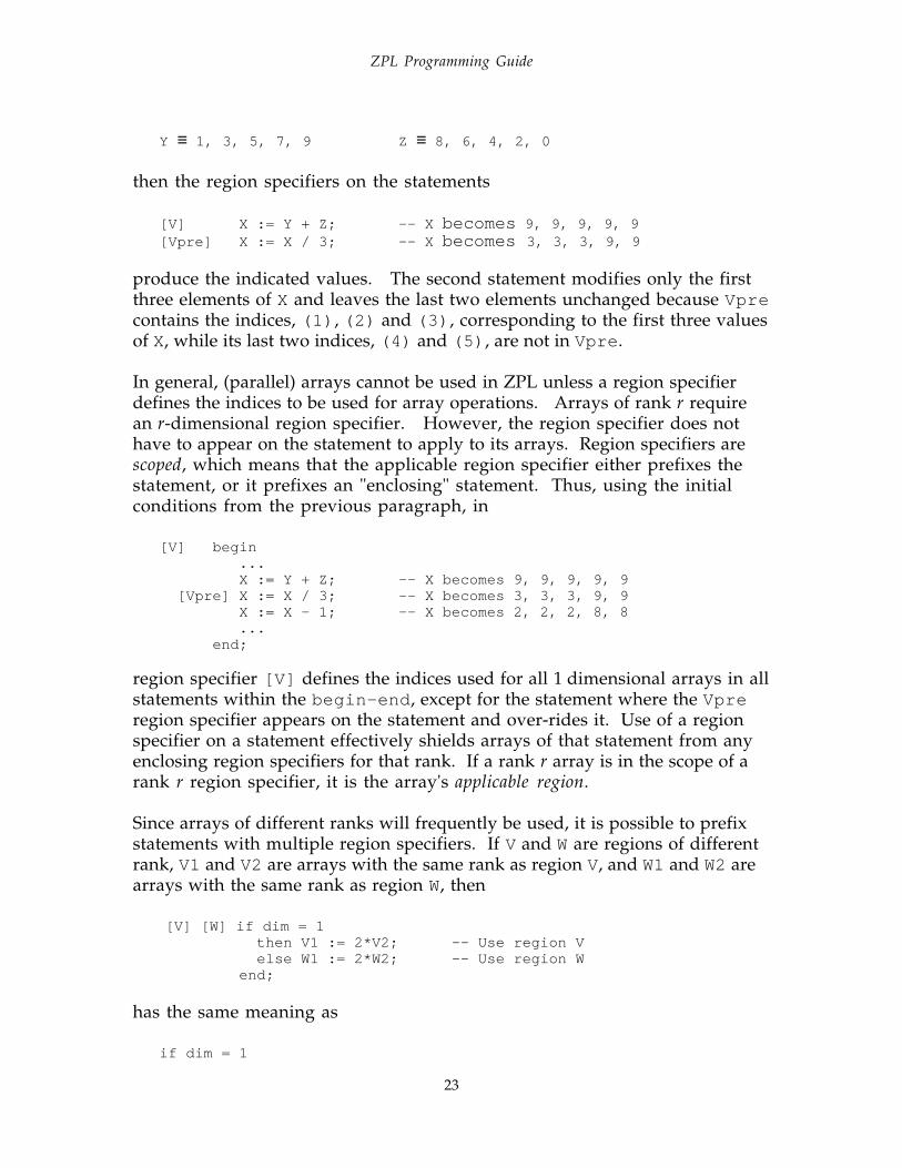
Y ≡ 1, 3, 5, 7, 9 Z ≡ 8, 6, 4, 2, 0
then the region specifiers on the statements
[V] X := Y + Z; -- X becomes 9, 9, 9, 9, 9[Vpre] X := X / 3; -- X becomes 3, 3, 3, 9, 9
produce the indicated values. The second statement modifies only the firstthree elements of X and leaves the last two elements unchanged because Vprecontains the indices, (1) , (2) and (3) , corresponding to the first three valuesof X, while its last two indices, (4) and (5) , are not in Vpre .
In general, (parallel) arrays cannot be used in ZPL unless a region specifierdefines the indices to be used for array operations. Arrays of rank r requirean r-dimensional region specifier. However, the region specifier does nothave to appear on the statement to apply to its arrays. Region specifiers arescoped, which means that the applicable region specifier either prefixes thestatement, or it prefixes an "enclosing" statement. Thus, using the initialconditions from the previous paragraph, in
[V] begin...X := Y + Z; -- X becomes 9, 9, 9, 9, 9
[Vpre] X := X / 3; -- X becomes 3, 3, 3, 9, 9X := X - 1; -- X becomes 2, 2, 2, 8, 8...
end;
region specifier [V] defines the indices used for all 1 dimensional arrays in allstatements within the begin-end , except for the statement where the Vpreregion specifier appears on the statement and over-rides it. Use of a regionspecifier on a statement effectively shields arrays of that statement from anyenclosing region specifiers for that rank. If a rank r array is in the scope of arank r region specifier, it is the array's applicable region.
Since arrays of different ranks will frequently be used, it is possible to prefixstatements with multiple region specifiers. If V and W are regions of differentrank, V1 and V2 are arrays with the same rank as region V, and W1 and W2 arearrays with the same rank as region W, then
[V] [W] if dim = 1 then V1 := 2*V2; -- Use region V else W1 := 2*W2; -- Use region Wend;
has the same meaning as
if dim = 1
ZPL Programming Guide
24
then [V] V1 := 2*V2; else [W] W1 := 2*W2;
end;
assuming that the dim variable is a scalar. That is, the statement in the then -clause will use the [V] region specifier since in either case -- whetherprefixing the statement or prefixing an enclosing statement -- thecomputation involving V1 and V2 is in its scope.
Finally, the region specifiers of statements can take a variety of forms,including dynamic regions, as described in Chapter 5.
Directions
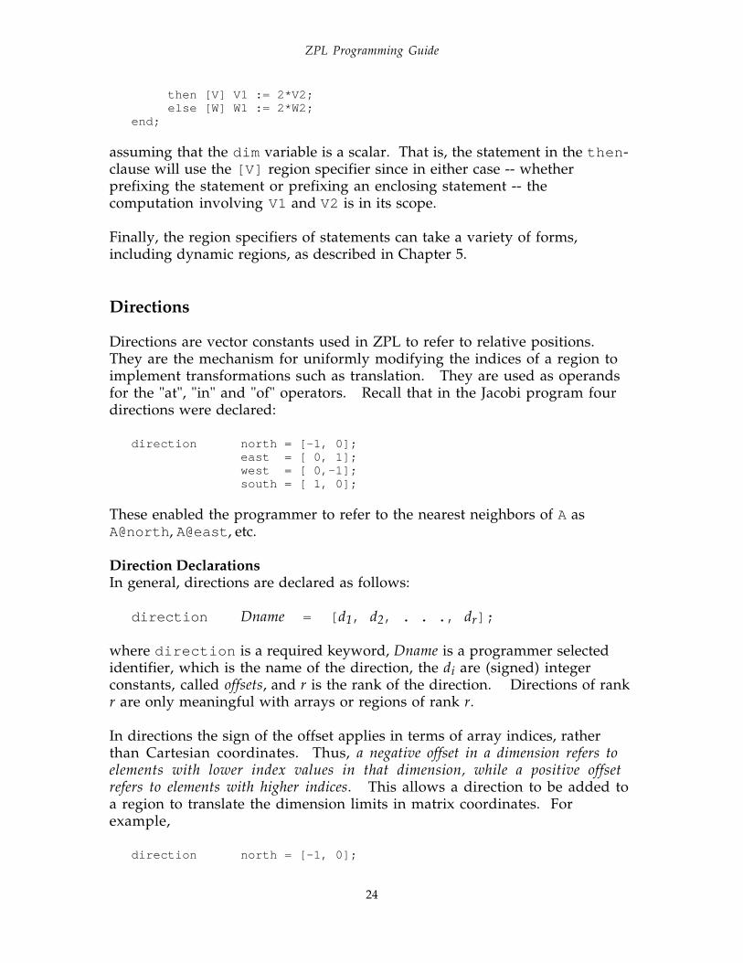
Directions are vector constants used in ZPL to refer to relative positions.They are the mechanism for uniformly modifying the indices of a region toimplement transformations such as translation. They are used as operandsfor the "at", "in" and "of" operators. Recall that in the Jacobi program fourdirections were declared:
direction north = [-1, 0];east = [ 0, 1];west = [ 0,-1];south = [ 1, 0];
These enabled the programmer to refer to the nearest neighbors of A asA@north , A@east, etc.
Direction DeclarationsIn general, directions are declared as follows:
direction Dname = [ d1, d2, . . ., dr];
where direction is a required keyword, Dname is a programmer selectedidentifier, which is the name of the direction, the di are (signed) integerconstants, called offsets, and r is the rank of the direction. Directions of rankr are only meaningful with arrays or regions of rank r.
In directions the sign of the offset applies in terms of array indices, ratherthan Cartesian coordinates. Thus, a negative offset in a dimension refers toelements with lower index values in that dimension, while a positive offsetrefers to elements with higher indices. This allows a direction to be added toa region to translate the dimension limits in matrix coordinates. Forexample,
direction north = [-1, 0];

ZPL Programming Guide
25
refers to the position "above" in relative orientation in a two dimensionalarray. As explained below, terms like "above" will be relative to arraycoordinates, but this does not preclude a Cartesian interpretation.
Directions are "not first class" so, once declared, they cannot be changed,assigned to variables, or passed to or from procedures.
Using Directions with "of"It is often convenient to define one region from another. The most commonexample is when a border is being defined for an array. The "of" operatoruses a direction and a region to define a new region adjacent to a previouslydefined region. The general form is
[ d of R]
where d is a direction and R is a region, called the base region. The semanticsare to define a new set of indices relative to R. Let
R = [l1..u1, l2..u2, . . ., lr..ur]
and
d = [d1, d2, . . ., dr]
then the region defined by [d of R] has indices such that the ith coordinateranges over the interval [l..u] , where
[u i +1..u i +di ] if d i > 0[l..u] = [l i ..u i ] if d i = 0 (*)
[l i +di ..l i -1] if d i < 0
Thus, the sign of the direction determines whether the dimension isextended at the lower (negative) or the upper (positive) end of the baseregion's index range, and the magnitude indicates by how much; a zero valuein a direction indicates that the whole interval for that dimension isinherited from the base region. Figure 3.1 shows examples.
Although the regions defined by the "of" operation are simply index sets, e.g.the regions of Figure 3.1 define the following index sets,
[SW2 of R] ≡ [ 9..10, -1..0][E2 of R] ≡ [ 1.. 8, 9..10][Top of C] ≡ [ 1.. 4, 0..0, 1..5][Edge of C] ≡ [ 1.. 4, 6..6, 6..6]

ZPL Programming Guide
26
they differ in an important way from the equivalent regions declared directly.Specifically, because "of" regions specify the region relative to a base region,they can be used to give arrays borders. That is, when an array is declaredover the base region and is then used in the context of an "of" region definedrelative to that base region, the referenced elements are treated as part of thearray. For example, using the definitions from Figure 3.1, and assuming A andB are declared over the base region R,
[E2 of R] A := 0.1; -- Initialize border columns to east[E2 of R] B := c*A; -- Set B's border to A's scaled by c
reference the 9th and 10th columns of A and B. Though A and B were notoriginally declared to have these two columns, the use of the array names inthe context of an "of" region augments the arrays with the region [E2 of R] .Thus, when a problem has "boundary conditions," the "of" region canestablish bordering regions to hold the boundary values. It is not necessary(or advisable) to declare arrays "larger" to accommodate boundary values as isnecessary in Fortran or C.
R
[SW2 of R] [E2 o f R]
[Top of C]
C
[Edge of C ]
SW2 = [ 2 ,-2]E2 = [ 0 , 2]Top = [ 0 ,-1, 0]Edge = [ 0 , 1, 1]
Figure 3.1: Examples of applying "of" to regionsR=[1..8,1..8] and C=[1..4,1..5,1..5]
Summarizing, "of" defines a new region from a base region and a direction.The region is adjacent to and disjoint from the base in the given direction. Ifan "of" defines "new" indices for the variable on the left-hand side of theassignment on which it appears, storage is declared for those new borderindices automatically, provided the region of the "of" expression is the samesymbolic region name as was used to declare the array.
Using Directions with "@"The "@" operator is used to implement the concept of "offset-referencing" ortranslation of arrays. Thus, in the Jacobi program, references to the nearestneighbors of A's elements were expressed as A@north , A@east, A@west andA@south.
In general, the "@" operator performs a uniform translation of a region'sindices and then references those elements of the array. Thus, in theconstruction

ZPL Programming Guide
27
[R] . . . A@d . . .
the referenced elements of A (and possibly its borders) are those found byadding the direction d to each index tuple in R. The result of the expressionis an array of the rank, size and index set of R. Thus, assumingR=[1..5,1..8] , A is defined over R and has a one column eastern boundarydefined, and the value in each i,j position is j, then
[R] . . . A@E . . .
refers to the shaded items, given E = [0,1]
1 2 3 4 5 6 7 8 91 2 3 4 5 6 7 8 91 2 3 4 5 6 7 8 91 2 3 4 5 6 7 8 91 2 3 4 5 6 7 8 9
A =
It must be emphasized that the rank, size and index set of the result ofapplying the "@" operator are determined by the region specifier, not thearray. The array (and possibly its borders) simply supply the values to bereferenced. Thus, certain uses of "@" will not result in an "array shift" or aspill to a border. To illustrate, consider the declarations,
region R = [1..3, 1..n]; --A 3 x n region Mid = [2..2, 1..n]; --A 1 x n region
var A3, B3: [R] integer; --3 x n arrays
direction above = [-1, 0]; --Offset first index upbelow = [ 1, 0]; --Offset first index down
which in the following statement
[Mid] A3@above := B3@below;
assigns the third row of B3 to the first row of A3. The region Mid , which is aset of indices for the second row of the R region, is translated to indices for thefirst row by above and to indices for the last row by below . The elementstransferred have the rank, size and index set of Mid .
In most programming languages, such a translation would be realized byiteratively referencing each element of the array using one or more nestedloops, and for each tuple of indices, (i,j, ..., k), a constant offset would be addedwhen subscripting the array. ZPL's ability to operate on arrays in theirentirety saves the tedious looping, and the use of symbolically nameddirections, e.g. northeast , avoids common errors in computing offsets in thesubscripts, e.g. [i-1, j+1].
ZPL Programming Guide
28
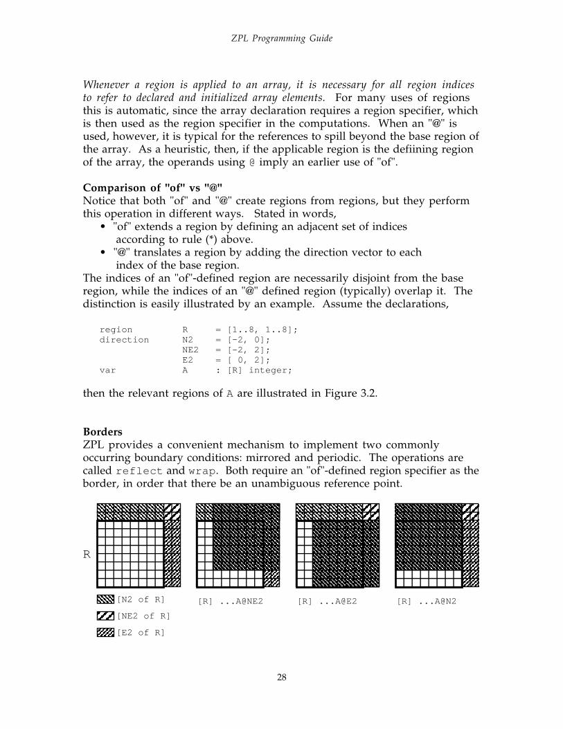
Whenever a region is applied to an array, it is necessary for all region indicesto refer to declared and initialized array elements. For many uses of regionsthis is automatic, since the array declaration requires a region specifier, whichis then used as the region specifier in the computations. When an "@" isused, however, it is typical for the references to spill beyond the base region ofthe array. As a heuristic, then, if the applicable region is the defiining regionof the array, the operands using @ imply an earlier use of "of".
Comparison of "of" vs "@"Notice that both "of" and "@" create regions from regions, but they performthis operation in different ways. Stated in words,
• "of" extends a region by defining an adjacent set of indicesaccording to rule (*) above.
• "@" translates a region by adding the direction vector to eachindex of the base region.
The indices of an "of"-defined region are necessarily disjoint from the baseregion, while the indices of an "@" defined region (typically) overlap it. Thedistinction is easily illustrated by an example. Assume the declarations,
region R = [1..8, 1..8];direction N2 = [-2, 0];
NE2 = [-2, 2]; E2 = [ 0, 2];
var A : [R] integer;
then the relevant regions of A are illustrated in Figure 3.2.
BordersZPL provides a convenient mechanism to implement two commonlyoccurring boundary conditions: mirrored and periodic. The operations arecalled reflect and wrap . Both require an "of"-defined region specifier as theborder, in order that there be an unambiguous reference point.
[N2 of R]
R
[NE2 of R]
[E2 of R]
[R] ...A@NE2 [R] ...A@E2 [R] ...A@N2

ZPL Programming Guide
29
Figure 3.2. Comparison of regions specified using "of" and "@"
The wrap operator has the general form
[ d of R] wrap vars;
where vars is a list of array identifiers, separated by commas. The effect ofapplying wrap to the d border of an array A is to set the border elements to bethe values from the "opposite" side of the array, that is, as if they "wraparound." See Figure 3.3. The general form of the reflect operation is
[ d of R] reflect vars;
where vars is a list of array identifiers, separated by commas. The effect ofapplying reflect to the d border of an array A is to set the elements of theboundary to be "mirrored around" the array's edge. See Figure 3.3.
A [E of R] wrap A; [E of R] reflect A;
Figure 3.3. Examples of wrap and reflect for a 2D array Aand direction E = [0,1] .
The operators are sufficiently intuitive that their rather complicated formaldefinitions will be omitted. Notice that in the figure, the "hatching" ismeaningful. That is, in wrap the data is translated, preserving order, whereasin reflect the data is mirrored, reversing the order.
Array and Cartesian Coordinates for DirectionsZPL's interpretation of directions in terms of array coordinates rather thanCartesian coordinates leads to the simple, uniform rule for describing thesemantics of region expressions: A negative offset in a dimension refers toelements with lower index values in that dimension, while a positive offsetrefers to elements with higher indices. This interpretation, however, troublessome first-time ZPL programmers, who prefer to think in Cartesiancoordinates. But, this is not a problem because ZPL programmers define theirown directions, and can therefore give them any meaning they wishprovided they are consistent. (This is why ZPL does not come with built-indirections.) For example, the declarations
region FQ = [0..n, 0..n]; -- An n+1 x n+1 regionvar Cart : [FQ] double; -- A variable declaration

ZPL Programming Guide
30
direction plusx = [ 1, 0]; -- Cartesian rightplusy = [ 0, 1]; -- Cartesian upminusx = [-1, 0]; -- Cartesian leftminusy = [ 0,-1]; -- Cartesian down
used consistently, allow the Cart array to be thought of as though it wereindexed like the first quadrant of the plane, i.e. the (0,0) element isconceptually in the lower left corner. So, for example,
[FQ] ... Cart@plusy ...
can be thought of as the array of values translated one unit in the upward(positive y) direction of the plane, because when thinking of FQ as the latticepoints in the first quadrant, [0,1] translates the points upwards. The factthat the ZPL compiler writers and possibly even the compiler itself interpretthis differently is irrelevant. The association of the letter sequence "plusy "or "east " to [0,1] is completely arbitrary; it could be "moonward " or"bzz333 ". If the Cartesian interpretation is used consistently, nocomputational problems should arise.* Accordingly, programmers areencouraged to adopt whatever interpretation makes sense to them, and toinclude a comment to assist anyone who reads the program.
Promotion
Scalars can be used throughout ZPL as if they were arrays of the rank, size andindex set of the region specifier for the operand with which they arecomposed. Scalars used in this role are said to be promoted to arrays. Thus,in the expression from the Jacobi program,
[R] Temp := (A@north+A@east+A@west+A@south)/4.0;
the scalar constant 4.0 is promoted to an array, implementing elementwiseaveraging, i.e. it becomes an array of 4.0 's of the rank, size and shape of R.Scalar promotion applies to each occurrence, taking the form required by thesituation in which it is used. Thus, if c is a scalar variable in
if dim = 1 then [V] V1 := c*V2; else [W] W1 := c*W2;end;
* Probably the only way a consistent use of alternate directions can be "exposed" is with the useof I/O, which is transmitted with the right-most-dimensions-varying-fastest rule applied tothe least index of the region. Thus, in this example, the (0,0) element of Cart would beprinted first. Users adopting an alternative set of directions may wish to preserve the illusionby restructuring their arrays before printing, postprocessing the output off-line or simplyassuring that the visualization software accepts the ZPL output as given.

ZPL Programming Guide
31
the promotion is to an array of rank, size and index set of V in the then -clauseand to W in the else -clause. Scalar promotion does not apply to a scalar onthe left-hand side of an assignment statement. Thus
[R] c := A; -- ILLEGAL, scalar promotion not allowed on lhs
is not legal. (See the reduce operator below.)
Promotion also applies to sequential functions. Examples of sequentialfunctions are the built-in numerical functions such as sin() , or user definedfunctions not employing array concepts in their definitions, e.g. conceptsdefined in this chapter. For example, in the statement
err := max<< abs(A - Temp);
from the Jacobi program, the (floating point) absolute value function, abs , ispromoted to accept an array, the result of A-Temp, as its actual parameter. Aswith variable promotion, function promotion applies to each occurrence, asthe situation requires. The meaning is to apply the scalar function to theoperand(s) for each index value of the region, i.e. elementwise.
Index1, Index2, ...
In ZPL (parallel) arrays cannot be explicitly indexed. This provides asignificant amount of "under constrained" computation for which a compilercan plan efficient execution. This is one of the properties of ZPL that allows itto execute fast on parallel computers. However, it is often useful to use theindex value in a computation. For this reason there are compiler-providedconstant arrays, known as Index d, that contain in each indexed position avalue of that index. (There are also "indexed" arrays," discussed in Chapter5.)
For example, assuming V is a one dimensional region, V = [1..n] , and V1 isa one dimensional variable defined over V, then the occurrence of Index1 inthe statement
[V] . . . V1 + Index1 . . .
is an n element vector containing in the ith position the value i, i.e.
Index1 ≡ 1 2 3 . . . n
In this case the Index d arrays are constant, they cannot be modified. Thus,constructions like
Index1 := . . .; -- ILLEGAL, cannot modify Indexd

ZPL Programming Guide
32
are prohibited.
In general, the Index d constant arrays are used by replacing d with anumerical value, say 2, specifying a dimension. The options are, therefore,
Index1 dimension 1 indicesIndex2 dimension 2 indicesIndex3 dimension 3 indices
. . .Indexd dimension d indices
. . .Indexr dimension r indices
where r is the highest dimension of any declared region of the program.Clearly, the r limit can be different for different programs.
The value of Index d is an array of the indices of the d dimension asdetermined by context. Thus, the shape and size of the array are the shapeand size of the operand region applicable to the operand with which it isbeing combined. For example, if R = [1..3, 1..4] is a rank 2 region andAny is a two dimensional array over these indices, then
[R] ... Any + Index1 ...
adds the row index to each element of Any , i.e. in this instance Index1 has thevalue
1 1 1 12 2 2 23 3 3 3
Contrast this with the occurrence of Index1 applied to a rank 1 array above.In each case, the shape and size of the Index d constant array are given by theshape and size of R, the applicable region for the variable with which it iscomposed.
Continuing the example,
[R] ... Any + Index2 ...
adds the column index to each element of Any , i.e. in this instance Index2has the value
1 2 3 41 2 3 41 2 3 4

ZPL Programming Guide
33
So, Index d extracts the dth items from the index tuple.
In general, if Index d is combined with an operand of rank r, the applicableregion specifier that determines Index d's size and shape is the rank r regionspecifier. (It is an error if d > r.) As a further example, if V = [1..n] is aregion, and V1 and V2 are rank 1 arrays, and W = [-5..5, 1..5] is a regionand W1 and W2 are rank 2 arrays, then the statement
[V][W] if dim = 1then V1 := Index1*V2; -- Ref 1D indiceselse W1 := Index1*W2; -- Ref first dim indices
end;
causes (among other things) the first element of V2 to be multiplied by 1 ifdim = 1 , or the first element of W2 to be multiplied by -5 otherwise.
For a square region R = [1..n, 1..n] , the statement
[R] Identity := Index1=Index2;
results in the identity matrix,
1 0 0 00 1 0 00 0 1 00 0 0 1
when n = 4, since the comparison of the Index d values is true (1) only on thediagonal.
The Index d constant arrays can be used in assignment statements,
[R] X := Index2; -- Set X to second dim indices
where the applicable region specifier is given by the left-hand side variable.Since the shape and size of an Index d constant array are determined by theoperand with which it is composed, there are a few cases where the applicableregion specifier cannot be inferred, e.g.
s := +<<Index1; -- Undefined use of Index1
and so the value is undefined.
Finally, it is frequently useful to initialize a multi-dimensional array suchthat in the ith position enumerated, say, in row-major order there is thevalue i. Row-major-order enumerates the items so the right-most indiceschange fastest, e.g. like an odometer. This can be computed easily and

ZPL Programming Guide
34
efficiently using the Index d arrays. Assuming R is a region with 1-originindexing, i.e. the indices in each dimension begin with 1, the statement
[R] Irmo := (Index1-1)*dim2size+Index2; -- Init. to row-major indices
produces the array
1 2 3 45 6 7 89 10 11 12
if dim2size ≡ 4. If R is not 1-origin, then the obvious corrections are required.
Index d arrays are only logicial. The compiler does not allocate memory orexplicitly create the Index d arrays, so they are very efficient to use.
Reduce and Scan
ZPL has two functional forms that can be used in global computations: reduceand scan. Both forms apply a function accumulatively to an array argument.Thus, +<<A finds the sum of the elements in A, i.e. reduces A to its sum. Theforms are as follows:
Reduce Name Scan +<< plus +|| *<< times *||max<< maximum max||min<< minimum min|| &<< and &|| |<< or |||
In general, for an array A the result of op||A is an array of the shape and sizeof the applicable region in which the ith element is the op -accumulation ofthe first i elements of the array, where the ordering is given by row-majororder. Thus, if for the applicable region of A
A ≡ 1 2 31 2 3
then the plus-scan of A
+|| A ≡ 1 3 6 7 9 12
and
max || A ≡ 1 2 3 min || A ≡ 1 1 1

ZPL Programming Guide
35
3 3 3 1 1 1
In general, for an array A, the result of the reduction op<<A is a scalar that isthe op -accumulation of the whole array, i.e. the last element of op||A . Thus,+<<A ≡ 12 , max<<A ≡ 3 , and min<<A ≡ 1 , given the previous definition ofA.
The operations available for use with scan and reduce are associative andcommutative as mathematical operations. They are treated as such in ZPL,i.e. the compiler reserves the right to accumulate the elements in any orderthat realizes the definition. However, in the finite precision of floating pointarithmetic, associativity is not strictly true for plus and times under allcircumstances.
The default is to apply reduce and scan to the entire applicable region of theoperand. In addition, a partial reduce or partial scan can be specified tooperate on a subset of the dimensions.
Partial scan is expressed by placing dimension specifiers -- dimensionnumbers in square brackets -- to the right of the function symbol, before theoperand. The specifier indicates which dimension(s) are to be scanned.Thus,
ColSum := + || [1] A; -- Add columns
is a plus-scan along the first dimension, i.e. the columns are added, assumingA is 2D. As expected, a partial scan will produce a result that is the sameshape and size as the operand. Partial reduce is slightly more complicated,since the number of dimensions in the result is logically smaller than theoperand, and so it is treated in Chapter 5.
If more than one dimension are to be partially scanned, the items in bracketsare separated by commas, e.g. +||[1,2] A . The dimensions are scanned inthe (left-to-right) order given in brackets. Since "wrapping" is part ofscanning, the order that the dimensions are scanned matters. See Figure 3.4.Thus, for 2D arrays, op||[2,1] gives a row-major order complete op -scan,i.e. is equivalent to op|| , and op||[1,2] gives a column-major ordercomplete op -scan. These are different from the consecutive application of onedimensional scans, since separate scans will not wrap. Notice that asmathematical operations the different orders of application of consecutiveseparate scans are all equivalent. This is not strictly true in the finiteprecision of a computer's floating point arithmetic.
To summarize, Figure 3.4 gives the logical order of accumulation for partialscan operations.

ZPL Programming Guide
36
1 1 1 1 1 2 3 4 1 1 1 1 1 2 3 41 1 1 1 1 2 3 4 2 2 2 2 5 6 7 81 1 1 1 1 2 3 4 3 3 3 3 9 10 11 12 A + || [2]A + || [1]A + || A
1 2 3 4 1 4 7 10 1 2 3 4 1 2 3 45 6 7 8 2 5 8 11 2 4 6 8 2 4 6 89 10 11 12 3 6 9 12 3 6 9 12 3 6 9 12 +||[2,1]A +||[1,2]A +||[1](+||[2]) ≡ +||[2](+||[1]A)
Figure 3.4. Logical order of accumulation for scan.

ZPL Programming Guide
37
-- Chapter 4 --
Program Structure and Examples
The goal of this chapter is to illustrate the constructs presented in the lastchapter, and to introduce ZPL programming idioms and style. In order toenable readers to run sample programs, basics of program structure and I/Oare treated first.
ZPL Programs
Though there is considerable flexibility in how ZPL programs are organized,the programmer must observe a few rules regarding program structure.Figure 4.1 shows the general schema of a ZPL program.
program Pname;
{config var declarations; } --{constant declarations; } --{type declarations; } --{direction declarations; } -- Preamble{region declarations; } --{var declarations; } --{Procedure_definitions; } --
procedure Pname(); -- Entry point procedureMain_program_definition ;
Figure 4.1. Structure of ZPL programs
In the schema the non-italic text must be given literally, including thepunctuation. The italicized text is to be replaced with syntactically correctcode meeting the italicized description. Items in braces are optional. Pnameis an identifier that is the name of the program, and must match in its twooccurrences. The Preamble items can appear in any order. Notice how theJacobi computation of Figure 1.2 fits into this structure.
The config var declaration section is used to specify parameters to thecomputation such as array sizes, convergence tolerances, etc. The configvar parameters are assigned default values in the declaration that can bechanged on the command line when the program is invoked. This allows

ZPL Programming Guide
38
the program to vary from run to run without recompilation. The declarationhas the form
config varident1 : type1 = val1;
...identn : typen = valn;
where the italicized material must be replaced as follows: identi is anidentifier, typei is its value type (see Chapter 2), and vali is its default value, tobe used unless changed at execution time. The config var parameters canbe used throughout the program, including in the remaining declarations,but they cannot be changed, i.e. they cannot appear on the left-hand side of anassignment, nor be passed as var parameters to a procedure, see Chapter 5.
To change the value of a config var on the command line for UNIXsystems, use the syntax
-s name=val
for each configuration variable name that is to be assigned a new val. Thus,for the Jacobi Iteration in Figure 1.2, which has the configuration variables nand delta , the invocation
jacobi -sn=25 -sdelta=.0001
resets both variables to new values. Further details on changing the defaultvalues of config var parameters are available as part of the compilerinstallation documentation.
Following the configuration variables are other global declarations, includingconstant declarations, region declarations (Chapter 3), type declarations(Chapter 5), direction declarations (Chapter 3), and var declarations. Theconstant declarations have the same form as the config var declarationsabove, e.g.
constant sisters : integer = 7;
and the var declarations simply list the variables of each type.
Though these declarations can be dense lists, it is recommendedprogramming style to consider how formatting might make the variableenumeration clearer. For example,
var x_x_,x0x_,x_x0,x0x0,x_y_,x0y_,x_y0,x0y0:sbyte;
is identical to

ZPL Programming Guide
39
var x_x_, x_y_, -- not presentx0x_, x0y_, -- single leftx_x0, x_y0, -- single rightx0x0, x0y0: -- filled
sbyte; -- range is -128 to 127
except for comments and white space, but the formatting improves thereadability, makes it easier to verify that there are no notational errors, andprovides information to the program reader.
The procedures of the program are declared at this point. One of theprocedures, usually the last or the first to be declared, is the procedure whosename is the same as the program. This is the main program or "entry point"procedure, i.e. the place where the computation begins.
The config var , constant , type , region , and direction declarations areglobal to the program, and are therefore declared before the proceduredeclarations. Variables can be declared either in the preamble or in theprocedures, including the main procedure. Most scientific and engineeringcomputations will have global variables representing the problem state.These are usually referenced by most or many of the program's procedures,and their space needs may dominate the memory requirements of theprogram. It is common to declare these variables in the preamble as part ofthe context of the computation, and to declare all other variables within theprocedures.
All ZPL source code must appear in a single file, though files can be included.That is, a line of the form
#include " filename"
will be replaced by the text in the file filename in the ZPL source file at the siteof the statement. Separate compilation is not presently supported.
Basic I/O
Programs must print out results, and most must also read in data. ZPLprovides input/output facilities, the most basic forms of which are treatedhere.
Text I/O Because ZPL operates in a UNIX environment, three files are alwaysopen, zin , zout and zerr , coresponding to UNIX's stdin , stdout andstderr . Programs can use other files for input and output by declaring avariable of type file ,

ZPL Programming Guide
40
var f : file; -- Declare variable for file descriptor
which is used to hold a file's descriptor. The file descriptor is set using theopen() procedure,
f := open("exprdata", "r");-- Open a file for reading
where the first parameter is the name of the file in quotation marks, and thesecond parameter is one of three alternatives, "r" , "w" , "a" , stating that datais to be read, written or appended to the file. The open() procedure returns adescriptor for the file that is to be used for all subsequent references to the file,or 0 if the opening operation was unsuccessful, e.g. the file could not befound. Notice that open() is not a parallel procedure, so it requires noregion.
Data is read from or written to files using the procedures,
read({ file,} vars) ;write({ file,} vars);writeln({ file,} vars);
where file is the optional file descriptor, and vars is a list of identifier namesparticipating in the I/O, separated by commas. If the file descriptor is notspecified, zin is used for reading and zout is used for writing. The write()and writeln() procedures differ only in that the latter writes a newlinecharacter after all of the variables are written.
The vars list can contain either sequential or parallel variable names. If(parallel) arrays are given, then appropriate region specifiers must apply tothe statements. The entire applicable region of the array is read or written,with the items assigned positions in row-major order, or more generally inrightmost-index-changes-fastest order. For example,
read(n); -- Get problem size from zin[R] read(f, A); -- Fill region R of A from file f[R] write(fdata, Alast); -- Save results in output file[V] writeln("Control Vector: ", C); -- Echo inputs to zout
writeln("MegaFLOPS :", f10to6); -- Report performance
are sample input/output statements.
Files other than zin and zout should be closed after their last use. Thecommand is close( file), where file is the file descriptor returned from theopen() command. So,
close(f); -- Finish up with file f
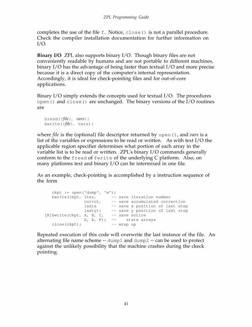
ZPL Programming Guide
41
completes the use of the file f . Notice, close() is not a parallel procedure.Check the compiler installation documentation for further information onI/O.
Binary I/O ZPL also supports binary I/O. Though binary files are notconveniently readable by humans and are not portable to different machines,binary I/O has the advantage of being faster than textual I/O and more precisebecause it is a direct copy of the computer's internal representation.Accordingly, it is ideal for check-pointing files and for out-of-coreapplications.
Binary I/O simply extends the concepts used for textual I/O. The proceduresopen() and close() are unchanged. The binary versions of the I/O routinesare
bread({ file}, vars);bwrite({ file}, vars);
where file is the (optional) file descriptor returned by open() , and vars is alist of the variables or expressions to be read or written. As with text I/O theapplicable region specifier determines what portion of each array in thevariable list is to be read or written. ZPL's binary I/O commands generallyconform to the fread of fwrite of the underlying C platform. Also, onmany platforms text and binary I/O can be intermixed in one file.
As an example, check-pointing is accomplished by a instruction sequence ofthe form
ckpt := open("dump", "w");bwrite(ckpt, iter, -- save iteration number
corrct, -- save accumulated correction lastx -- save x position of last step lasty); -- save y position of last step
[R]bwrite(ckpt, A, B, C, -- save entire D, E, F); -- state arrays
close(ckpt); -- wrap up
Repeated execution of this code will overwrite the last instance of the file. Analternating file name scheme -- dump1 and dump2 -- can be used to protectagainst the unlikely possibility that the machine crashes during the ckeckpointing.

ZPL Programming Guide
42
Example Computations
In this section ZPL will be used to solve "typical" scientific and engineeringcalculations. The emphasis is on illustrating standard ZPL idioms, i.e.showing characteristic constructs and styles for solving problems:
• Computing over entire arrays without any indexing.• Substituting computations over logical vectors for if statements.• Comparing alternative solutions based on expected performance.
Though these techniques are highlighted here, they are all intuitive, andeasily understood and used.
Sample StatisticsThe computation to be illustrated is that of finding the mean and standarddeviation of a set of data values. The overall structure of the program is toread the data, compute the statistics, and print the results. The program isshown in Figure 4.2.
The programmer has defined items , the size of the problem, to have thedefault value 100, and this value is used to declare the region R. No directiondeclarations are needed for this calculation. In the header of the mainprocedure Sample is declared together with two scalars, mu and sigma . Thestatistics are computed by a direct application of their defining formulae.
1 program Sample_Stats; 2 /* Program computing the mean and standard deviation of a sample */ 3 4 config var items : integer = 100; -- Problem size 5 region R = [1..items]; -- Problem space 6 7 procedure Sample_Stats(); -- Start of Program 8 var Sample : [R] float; -- Declare data array 9 mu, sigma : float; -- Declare scalars1011 [R]begin12 read(Sample); -- Input from zin13 mu := +<<(Sample/n); -- Mean14 sigma := sqrt(+<<((Sample-mu)^2/n)); -- Std deviation15 writeln("Mean: ", mu); -- Print16 writeln("Standard Deviation: ", sigma); -- results17 end;
Figure 4.2. Sample statistics program.
The mean, µ, defined as

ZPL Programming Guide
43
µ = ∑ i Samplei /n
is computed by
mu := +<<(Sample/n); -- Mean
where the summation is accomplished by the plus-reduction operation overthe Sample array. Notice that because of the precedence of the operators(Table 2.1), the plus-reduction binds more tightly than the division, soparentheses are required for each Sample item to be divided by n.Eliminating the parentheses performs a single division after summingSample , which may be somewhat more precise at the risk of a greaterpossibility of overflow. Parentheses showing the groupings arerecommended as good programming practice.
The standard deviation, σ, defined as ____________________σ = √ ∑i (Samplei - µ)2/n
is translated directly into
sigma := sqrt(+<<((Sample-mu)^2/n)); -- Std deviation
where the sqrt function computes the square root. Notice that subtractingmu from Sample has the effect of promoting the scalar to an array with shapeand size given by [R] , and then subtracting corresponding elements. Theresults are printed and the program exits.
Correlation CoefficientFigure 4.3 illustrates a program that is quite similar to Sample_Stats .Coefficient finds the means of two samples and computes their correlationcoefficient,
Σ i (Sample1i - µ1)(Sample2i - µ2)r = ---------------------------------------------------------------
√ Σ i (Sample1i - µ1)2 ⋅ Σ i (Sample2i - µ2)2
on Lines 19-20.
One difference with Sample_Stat is that Coefficient reads in its data fromfiles. The files, which are expected to be called "Expr1 " and "Expr2 ," arespecified by a call to the procedure open() that returns a file descriptor. Thisis assigned to a variable of type file , and used in the subsequent read() and

ZPL Programming Guide
44
close() procedures. Though the program works if the files are not closedbefore exit, it is a good policy to do so. As before, the results are written tozout , since no file is specified in the writeln() statements.
The program is very similar to Sample_Stats . All computation in the bodyis performed within the scope of the region specifier [V] , so all arrayoperations apply to all n items of the two arrays. In lines 15-16 the plus-reduction operation is used to sum the elements to compute the two means.Then, in lines 17-18 these means are promoted to n element arrays to matchthe Sample arrays, and corresponding elements are subtracted. Analternative way to express these two computations employs ZPL's extendedassignment operators,
Sample1 -= mu1; -- Center about meanSample2 -= mu2; -- Same for next sample
The correlation coefficient is computed in an expression that breaks acrosslines 19-20. Notice that the second line starts with the divide operator. It ishelpful to begin continuation lines with an operator as a visual cue toindicate a multiline statement, but of course, it is not required. Finally, theresults are printed out.
1 program Coefficient; 2 /* Compute the means and correlation coefficient of two samples */ 3 4 config var items : integer = 100; -- Problem size 5 region V = [1..items]; -- Problem space 6 7 procedure Coefficient(); -- Start of Program 8 var Sample1, Sample2 : [V] float; -- Declare data array 9 mu1, mu2, r : float; -- Declare scalars10 f1, f2 : file; -- File name variables1112 [V]begin13 f1 := open("Expr1","r"); read(f1,Sample1);--Data from file Expr114 f2 := open("Expr2","r"); read(f2,Sample2);--Data from file Expr215 mu1 := +<<(Sample1/n); -- First sample mean16 mu2 := +<<(Sample2/n); -- Second sample mean17 Sample1 := Sample1 - mu1; -- Center about mean18 Sample2 := Sample2 - mu2; -- Same for next sample19 r := (+<<(Sample1*Sample2)) -- Correlation coeff'nt20 / sqrt((+<<(Sample1^2))*(+<<(Sample2^2)));21 writeln("Sample means: ", mu1, mu2); -- Print22 writeln("Correlation coefficient: ", r); -- results23 close(f1); close(f2); -- Wrap up for exit24 end;
Figure 4.3. Computing the correlation coefficient

ZPL Programming Guide
45
HistogramComputing the values for a histogram of a data set is straightforward. Firstthe interval spanned by the entire data set of Values is found by determiningthe smallest and largest elements,
small := min<<Values;big := max<<Values;
using the reduction operators. If this range is to be divided into b equal sizebins, then each bin has a size determined by
size := (big - small)/b;
To assign the Values to one of the b equal sized bins, it is expedient to shiftthe values by subtracting small so the smallest is zero, then to divide thesize into each item,
BinNo := ceil((Values-small)/size);
rounding-up the fractional part to the next highest integer. This results inBinNo i containing the bin number for Values i.
This assigns each of the Values to the proper bin except those items equal tosmall , the low end point of the whole interval. They are assigned to thenonexistent bin 0. Assuming such elements are to be assigned to bin 1, it isnecessary to increment all BinNo s having a value 0. It is possible to fix upthese entries with an if -statement that tests for 0 and then increments it. But,it is also possible to write
BinNo := BinNo + !BinNo; -- Put "small" elements in bin 1
which uses the fact that nonzero BinNo values are treated as logical true and 0BinNo values are treated as logical false. Thus, the negation !BinNo yields avector of trues (1) and falses (0) where 0s and nonzeroes occur in BinNo . Byadding these to BinNo , the 0s are incremented.
For example, if
b ≡ 3 and Values ≡ 6.3 -4.2 0.0 1.9 5.4 -2.2 -4.2 -2.2
then
small := min<<Values; -- small ≡ -4.2big := max<<Values; -- big ≡ 6.3size := (big-small)/b; -- size ≡ 3.5BinNo := ceil((Values-small)/size);-- BinNo ≡ 3 0 2 2 3 1 0 1BinNo := BinNo + !BinNo; -- !BinNo ≡ 0 1 0 0 0 0 1 0

ZPL Programming Guide
46
producing a final value
BinNo ≡ 3 1 2 2 3 1 1 1
as intended.
This programming technique -- using the addition of a Boolean vector as asubstitute for an if -statement -- is an example of computing with logicalvectors. This is a recommended approach not only because of the clean andsuccinct program, it uses computation instead of control to achieve the result.Since modern pipelined computers are slowed by the "control jumps" typicalof if -statements, using logical vectors will likely result in faster code.
1 program Histo; 2 /* 3 The n nonegative values read from zin are grouped into b equal 4 sized intervals over their range, counted and printed out. 5 Values on the boundaries are associated with the higher interval. 6 */ 7 config var n : integer = 100; -- Size of data 8 b : integer = 8; -- Number of intervals in histogram 9 region S = [1..n]; -- The index space of the data1011 procedure Histo(); -- Entry point12 var small, -- Smallest value13 big, -- Largest value14 size : float; -- Interval size of bin15 count, i : integer; -- Integer scalars16 Values : [S] float; -- Data value array17 BinNo : [S] ushortint; -- Bin numbers are nonnegative1819 [S]begin20 read(Values); -- Get the data from zin21 small := min<<Values; -- Get smallest value22 big := max<<Values; -- Get largest value23 size := (big-small)/b; -- Figure size of the intervals24 BinNo := ceil((Values-small)/size);25 -- Compute position, round up26 BinNo := BinNo + !BinNo; --Include lo endpoints in first bin27 writeln("Histogram of ", n,28 " values, ranging from ", small,29 " to ", big,30 " grouped into ", b,31 " intervals of size ", size);32 for i := 1 to b do33 count := +<<(BinNo = i); -- Count how many in this interval34 writeln("Interval ",small + (i-1)*size,35 " : ", small + i*size,36 " = ", count);37 end;38 end;
Figure 4.4. Program to print the count of samples in b equal-sized bins.

ZPL Programming Guide
47
In the Histo program shown in Figure 4.4 there is a second application ofcomputing with logical vectors. After writing out the header information forthe computation (lines 27-31), a for -loop is entered in which on the i th
iteration, the number of elements in bin i are counted and then printed. Tocount the number of elements in bin i , BinNo is compared to i producing alogical vector over which a sum reduction is applied yielding the number ofelements in the bin
count := +<<(BinNo = i);
Again, this is an efficient alternative to the use of an if -statement A variantof this histogram program is given in Chapter 6.
1 program UniConv_Shift; 2 config var N : integer = 512; -- No. pixels in 1 dim. 3 boxb : ushortint = 4; -- Default size box base 4 boxh : ushortint = 4; -- Default size box height 5 w : ushortint = 16; -- Default weight 6 filename : string = "Image"; -- Name of input file 7 region I = [1..N, 1..N]; -- Problem space 8 var Im : [I] ubyte; -- Image of pixels 9 BoxSum, T : [I] ushortint; -- Result and temp10 fptr : file; -- Unix file descriptor1112 direction west = [ 0,-1];13 north = [-1, 0];1415 procedure UniConv_Shift(); -- Entry point16 var i : integer; -- Loop variable1718 [I] begin -- Refer to entire image19 fptr := open(filename,"r");-- Locate the file20 read(fptr,Im); -- Get the image21 [west of I] T := 0; -- Init west boundary22 [north of I] T := 0; -- Init north boundary23 BoxSum := Im; -- Init BoxSum w/1st val24 T := Im; -- T will shift around25 for i := 1 to boxb - 1 do -- Across box ...26 T := T@west; -- Shift image L-to-R27 BoxSum := BoxSum + T; -- Accumulate28 end; -- ... sweep rows29 T := BoxSum; -- Init T w/ box row sums30 for i := 1 to boxh - 1 do -- Across box ...31 T := T@north; -- Shift row sums down32 BoxSum := BoxSum + T; -- Accumulate33 end; -- ... sweep columns34 BoxSum := BoxSum/w; -- Weight entries35 writeln(BoxSum); -- Print results to zout36 close(fptr); -- Close up37 end;
Figure 4.5. Shift and Add solution to uniform convolution

ZPL Programming Guide
48
Uniform Convolution
In this application the values stored in the 512×512 array are picture elementsor pixels. The uniform convolution problem is to treat every point in theimage as the lower right corner of a x×y box of pixels, and to store theweighted sum of the elements of the box into that position. Perhaps themost straightforward solution is to shift the array around, adding up thepixels. But there is an ingenious solution using the scan, which will also beconsidered.
Shift-and-Add SolutionThis solution of the uniform convolution computation conceptually shiftsthe image to the right, accumulating in each position the pixel values of therow to its left. These values, i.e. the box's row sums, are then shifted downand accumulated, scaled and written out. The program is shown in Figure4.5.
The program begins by defining the default sizes of the box base, boxb , boxheight, boxh , and weight, w, since these quantities will tend to be the samefrom run to run. By being declared as config var s, however, their valuescan be changed on the command line when the program is executed. Im isdeclared to be an unsigned byte array, allowing the pixels to have at most 256distinct values, and BoxSum, the array that will accumulate the values fromthe various positions, is declared ushortint . This specification allows forboxes with area up to 256 pixels without overflow, because if boxh × boxb =box area ≤ 256 then the
largest pixel value × box area ≤ 255 × 256 = (28-1) × 28 < 216-1
the typical precision of unsigned short integers. Notice that because BoxSum isan integer value, the scaling (Line 34) will truncate any fractional parts.
The program begins by opening a file that has the default name "Image ",which can be changed on the command line, and reading the contents intoIm .
The computation begins by initializing to 0 the west and north boundaries ofT, the copy of the image (and later the row sums) that will be shifted aroundto accomplish the summation. The shifting will first go to the right, and thendownwards, which means that 0's will be introduced into T from the westand north boundaries.
BoxSum is initialized to Im , which would be the final result for a degenerate1×1 box, and T is initialized to the image. Shifting to the right is implementedin the for -loop (Lines 25-28), yielding the effect of summing across the rows

ZPL Programming Guide
49
of a box of width boxb . This intermediate result is then assigned to T, and thecolumns are added up. Since the column above a given position contains thesums of the rows of the box, this produces the result, which is then scaled andwritten out.
1 program UniConv_Scan; 2 config var N : integer = 512; -- No. pixels in 1 dim. 3 w : integer = 16; -- Weight 4 region I = [1..N, 1..N]; -- Problem space 5 var Im : [I] ubyte; -- Image array 6 BoxSum : [I] uinteger; -- Result array 7 filename : string; -- Name of input file 8 fptr : file; -- Unix file descriptor 910 direction west = [ 0,-4]; --\11 north = [-4, 0]; -- Box specifications12 NW = [-4,-4]; --/1314 procedure UniConv_Scan(); -- Entry point15 [I] begin -- Refer to the entire image16 [west of I] BoxSum := 0; -- Initialize the17 [NW of I] BoxSum := 0; -- boundaries of the18 [north of I] BoxSum := 0; -- result to 019 write("Image? ");read(filename);--Get name from zin20 fptr := open(filename,"r");-- Locate the file21 read(fptr,Im); -- Get the image22 BoxSum := +||[2] Im; -- Find row sums23 BoxSum := +||[1] BoxSum;-- Find column sums24 BoxSum := BoxSum - BoxSum@north -- Correct row sums25 - BoxSum@west -- Correct column sums26 + BoxSum@NW; -- NW subt'd twice, add in27 BoxSum := BoxSum/w; -- Weight entries28 writeln(BoxSum); -- Print results to zout29 close(fptr); -- Button up30 end;
Figure 4.6. Scan solution for the uniform convolution.
Scan SolutionIf the box size can be fixed at compile time, the programmer has available analternative implementation based on the scan operation. Rather than addingup the rows and columns of the box, the basic idea is to use the scan to sumacross the rows and columns of the whole image, and to derive the BoxSum byperforming some simple arithmetic on these values. Figure 4.6 shows auniform convolution solution using scan for a fixed 4×4 box.
The first difference is that BoxSum must be declared to be an unsigned integer,because summing over the entire array means that the magnitudes of theintermediate terms can be larger than can be represented in a shortint . Asecond difference is that the declarations for the directions (Lines 10-12) arelarger. These correspond to the size of the box rather than the unit of motion

ZPL Programming Guide
50
as they did in the shift-and-add solution. When the border initialization isspecified (Lines 16-18), these directions produce somewhat "thicker" borders
0 0 0 00 0 0 00 0 0 00 0 0 00 0 0 00 0 0 0
0 0 0 0 0 0 0 0 0 00 0 0 0 0 0 0 0 0 00 0 0 0 0 0 0 0 0 00 0 0 0 0 0 0 0 0 0
BoxSum
than the 1-wide borders of the shift-and-add solution.
After reading in the image, the program proceeds to compute the row andcolumn sums using partial scans, i.e. scans that apply over one dimensiononly (Chapter 3). Recall that the dimension over which the sum isperformed is given in brackets (Lines 22-23), so +||[2] adds across rows,while, +||[1] adds down columns.
The logic of the computation is simple. By plus-scanning the rows of Im (Line22), and then plus-scanning the columns of that result (Line 23), each positioncontains the sum of itself and all pixels to the north and west. The values forthese elements are the sum of the entire array to their northwest. For allelements with indices larger than four in either dimension, this is too much.So, the value from four rows above is subtracted (Line 24), as is the value fourcolumns to the left (Line 25). However, this has subtracted the values to thenorthwest twice, so they must be added back in again (Line 26), as thefollowing example, using an array of 1 pixels, illustrates
1 1 1 1 1 1 1 2 3 4 5 6 1 1 1 1 1 1 1 2 3 4 5 6 1 1 1 1 1 1 1 2 3 4 5 6 1 1 1 1 1 1 1 2 3 4 5 6 1 1 1 1 1 1 1 2 3 4 5 6 Im Line 22
1 2 3 4 5 6 1 2 3 4 5 6 2 4 6 8 10 12 2 4 6 8 10 12 3 6 9 12 15 18 3 6 9 12 15 18 4 8 12 16 20 24 4 8 12 16 20 24 5 10 15 20 25 30 4 8 12 16 20 24 Line 23 Line 24

ZPL Programming Guide
51
1 2 3 4 4 4 1 2 3 4 5 5 2 4 6 8 8 8 2 4 6 8 8 8 3 6 9 12 12 12 3 6 9 12 12 12 4 8 12 16 16 16 4 8 12 16 16 16 4 8 12 16 15 14 4 8 12 16 16 16
Line 25 Line 26
Restoring the northwest component is required because the original value ofBoxSum, as of Line 23, is used throughout the computation of Lines 24-26. Asan exercise, the reader can verify that had the rows above and the columns tothe left been subtracted off in separate statements, say with
BoxSum := BoxSum - BoxSum@north;BoxSum := BoxSum - BoxSum@west;
no "northwest" correction would have been required. This is because theseparate statements update the Boxsum value.
If the box size is known at compile time, the programmer has a choice ofimplementations. Which is preferable depends on the box size. For smallboxes, e.g. 2×2, the shift solution is better since it reduces data motion. As thebox size grows, however, the pair of scans becomes more efficient.
Counting Connected ComponentsThe problem considered is counting the "connected components" of an imagethat is represented as a two dimensional array of binary pixels. Two 1's are inthe same connected component if there is a path between them composedonly of 1's, where the "steps" permitted in the path are any of the eightcompass directions. This is the 8-way connected components definition;there is also a 4-way definition as well.
The program to count 8-way connected components will illustrate how ZPLprogramming benefits from thinking globally. The solution [Cypher et al. 90]relies on the "amazing" shrinking operator due to Levialdi. Thismorphological transformation preserves connectedness while reducing thesize of a component. It is applied iteratively. The pixels are simultaneouslyrewritten to form the next iteration according to the following rule:
Levialdi Shrinking Operator (8-way): Pixels simultaneously change fromone iteration to the next according to the rule:
remains 1 if there is a 1 to its west, northwest or north, (1→1) (a)1 becomes 0 if there are 0's to its west, northwest and north (1→0) (b)
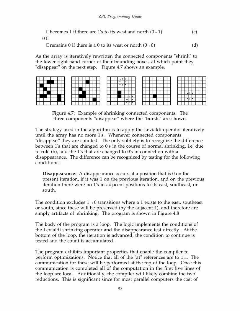
ZPL Programming Guide
52
becomes 1 if there are 1's to its west and north (0→1) (c)0 remains 0 if there is a 0 to its west or north (0→0) (d)
As the array is iteratively rewritten the connected components "shrink" tothe lower right-hand corner of their bounding boxes, at which point they"disappear" on the next step. Figure 4.7 shows an example.
Figure 4.7: Example of shrinking connected components. Thethree components "disappear" where the "bursts" are shown.
The strategy used in the algorithm is to apply the Levialdi operator iterativelyuntil the array has no more 1's. Whenever connected components"disappear" they are counted. The only subtlety is to recognize the differencebetween 1's that are changed to 0's in the course of normal shrinking, i.e. dueto rule (b), and the 1's that are changed to 0's in connection with adisappearance. The difference can be recognized by testing for the followingconditions:
Disappearance: A disappearance occurs at a position that is 0 on thepresent iteration, if it was 1 on the previous iteration, and on the previousiteration there were no 1's in adjacent positions to its east, southeast, orsouth.
The condition excludes 1→0 transitions where a 1 exists to the east, southeastor south, since these will be preserved (by the adjacent 1), and therefore aresimply artifacts of shrinking. The program is shown in Figure 4.8
The body of the program is a loop. The logic implements the conditions ofthe Levialdi shrinking operator and the disappearance test directly. At thebottom of the loop, the iteration is advanced, the condition to continue istested and the count is accumulated.
The program exhibits important properties that enable the compiler toperform optimizations. Notice that all of the "at" references are to Im . Thecommunication for these will be performed at the top of the loop. Once thiscommunication is completed all of the computation in the first five lines ofthe loop are local. Additionally, the compiler will likely combine the tworeductions. This is significant since for most parallel computers the cost of

ZPL Programming Guide
53
reduction is dominated by interprocessor communication, and since they canusually communicate two words for the same cost as communicating one,combining the two costs little more than a single reduction.
1 program CountCon; -- Count Connected Components 2 config var n : integer = 512; -- Image size in 1 dim. 3 region I = [1..n, 1..n]; -- Problem space 4 var Im, Conn, Next : [I] ubyte; -- Image arrays 5 6 direction north = [-1, 0]; NE = [-1, 1]; 7 east = [ 0, 1]; SE = [ 1, 1]; 8 west = [ 0,-1]; SW = [ 1,-1]; 9 south = [ 1, 0]; NW = [-1,-1];1011 procedure CountCon(); -- Entry point12 var smore : boolean; -- Loop control13 count : integer; -- Num components14 fptr : file; -- UNIX file pointer15 [I] begin16 [north of I] Im := 0; -- Set boundaries to 017 [NE of I] Im := 0; -- |18 [east of I] Im := 0; -- |19 [SE of I] Im := 0; -- |18 [west of I] Im := 0; -- |20 [SW of I] Im := 0; -- |21 [south of I] Im := 0; -- |22 [NW of I] Im := 0; -- V23 count := 0; -- Initialize count24 fptr := open("Image","r"); -- Find file25 read(fptr, Im); -- Get the image26 repeat -- Over all I, iterate27 Next := Im & (Im@north | Im@NW | Im@west);28 -- Apply rules (a), (b)29 Next := Next | (Im@west & Im@north & !Im);30 -- Apply rules (c), (d)31 Conn := Im@east | Im@SE | Im@south;32 -- Find the 1's33 -- preserving34 -- connectedness35 Conn := Im & !Next & !Conn;36 -- Check disappearance37 Im := Next; -- Advance iteration38 smore := |<<Im; -- Decide if continuing39 count += +<<Conn; -- Count all vanished40 -- this time41 until !smore; -- Stop when all zeroes42 writeln(count); -- Report results43 close(fptr); -- Close up44 end;
Figure 4.8. Connected components counting program using the Levialdishrinking operator.
Notice that although the two reductions can generally be combined by thecompiler to remove half of the communication overhead, the programmer

ZPL Programming Guide
54
could remove the reduction over Conn from the loop. Specifically, let Accumbe an array of ubyte s initialized to 0. Then, replacing line 39 by
Accum := Accum + Conn;
or its more succinct form
Accum += Conn;
the count of the components vanishing at a given position is kept. When theloop exits, the total can be computed by reducing Accum,
writeln(+<<Accum);
eliminating the need for the variable count at the expense of adding the arrayAccum.
References
R. E. Cypher, J. L. C. Sanz and L. Snyder, 1990. "Algorithms for ImageComponent Labeling on SIMD Mesh Connected Computers," IEEETransactions on Computers, 39(2):276-281.

ZPL Programming Guide
55
-- Chapter 5 --
Generalizing ZPL
In earlier chapters the basic array capabilities of ZPL were introduced. Manyof those features have more advanced forms, which will be described in thischapter. The following specific topics will be treated.
Additional Region SpecificationsDegenerate Ranges@ Compositions"At" In Region Specifiers"Of" Compositions"In" RegionsCombined Specifications
Dynamic RegionsInheritanceDitto
Indexed ArraysType DeclarationsFloodingReduction/Scan RevisitedRegion ConformanceProcedures
DeclarationsPrototypesCallsPromotionRecursion
Shattered Control FlowMasks
Familiarity with the basic concepts from previous chapters is assumed.
Additional Region Specifications
There are a variety of simplifications that make defining regions easier.
Degenerate RangesIn region specifications, a degenerate range, i.e. an index range of length 1, canbe specified simply by giving that item. (One is the minimum length of anyrange of a dense region. See below.) Thus,
region Col1 = [1..n, 1..1];

ZPL Programming Guide
56
is equivalent to
region Col1 = [1..n, 1];
The rule also applies for dynamic regions (see below).
@ CompositionsMultiple directions can be composed using @. For example, A@east@northhas the same meaning as A@northeast , assuming the directions have theirobvious definitions, north=[-1,0], east=[0,1], northeast=[-1,1] .The rule is that the resulting direction is found by adding the directions of thecomposition as vectors. Notice that because addition is commutative andassociative, the resulting direction is the same regardless of the order ofapplication, e.g. A@north@east ≡A@east@north . Accordingly, noparenthesization is necessary, nor is it allowed.
It is believed that a program's clarity is improved by declaring frequently useddirections rather than repeatedly composing them. However, for occasionaluse compositions allow the direct formation of specialized regions from basicparts.
"At" in Region SpecifiersSo far, @ has been used to translate arrays, but an analogous translation is alsoavailable for region specifiers using the letter sequence at . The symbols arerestricted: the letter sequence at is used in the region specifiers only, while @applies to array operands only. Thus, if west = [0,-1] and R = [1..n,1..n] , then
[R at west] . . .
specifies the region with a 0th column and no nth column. And in
[R at west] . . . A@east . . .
the R region of A is specified, assuming east = [0,1] . That is, thedirections cancel. Cancelling directions are useful, as illustrated in the"move particles" code in Chapter 9. Compositions are allowed with theregion specifier form of at , e.g. [R at east at north] is allowed. Like @compositions, the resultant direction is found by adding the directions asvectors. Parentheses are not necessary or allowed.
"Of" CompositionsMultiple directions can be composed using of . For example, east of northof R is equivalent to northeast of R , assuming the directions have theirobvious definitions given above. But the situation is more subtle than with

ZPL Programming Guide
57
the at . The rule for of computations is that the resulting region is found byevaluating the expression "inside-out," i.e. by applying the rightmostdirection to the region, and then working out. Thus, the foregoing expressionwould be evaluated as if it were east of (north of R) , althoughparenthesization is not permitted. The inside-out rule for of compositions isnatural: Since of is an operator taking both a direction and a region asoperands and yielding a region as a result, applying the inside-out rule to anof composition effectively collapses d of R to R', a new region, enabling thenext outer most application of of .
Notice that because of -regions are disjoint from their base regions,expressions that would seem to "cancel," e.g. west of east of R , can bemeaningful. So, assuming a 2D region R and the usual definitions fordirections, the region west of east of R refers to the last column of R.
"In" RegionsThe of operator constructs a border region that is adjacent to and just outsidethe edge of a base region. The in operator constructs a similar region justacross the edge on the "inside" of the base region. That is, if R = [1..n,1..n]
[east in R] . . .
refers to the last column of R, assuming east = [ 0, 1] . Also, assumingse = [ 1, 1]
[se in R] . . .
refers to the single element region {(n,n) } in the lower right corner of R.Notice that combinations of in are permitted without parentheses, allowing
[south in east in R] . . .
to be an alternative formulation for {(n,n) }. As with of , in combinationsare evaluated inside-out from the base region.
Combination SpecificationTwo classes of combinations are permitted: in and of specifications can bemixed on the left hand side of a base region, and at can be simultaneouslyapplied to a region that is constructed using in or of or a combination of thetwo.
To interpret a combination of in and of operators applied to a base region,evaluate them inside-out, just as with expressions composed exclusively ofin or of .

ZPL Programming Guide
58
For expressions containing at together with in or of , the region is found byapplying the inside-out rule to the region as modified by the composed at 's.Thus, if R is a rank 2 region
[east of south of R at north at west]
refers to the lower right corner index of R, since R at north at west shiftsthe array one position up and left, south of that region describes the last rowshifted one position left, and east of that is the element to its right, i.e. thelower right corner.
R
(a) (b) (c) (d) (e)
Figure 5.1. Combination of at and of . (a) Region R, (b) R at north ,(c) R at north at west , (d) south of R at north at west ,
(e) east of south of R at north at west .
As previously mentioned, clarity is likely promoted by declaring frequentlyused regions rather than repeatedly specifying them using compositions.
Dynamic Regions
Regions, as explained so far, allow index sets to be named, i.e. declared, and tobe formed by transformation using various prepositions. These are all staticspecifications of index sets in that once defined they are unchangeable. It isusually sensible to use statically known regions wherever possible, since ameaningful name can convey information to the programmer, there is lesschance of error, and the compiler may be able to apply more optimizations insuch cases. But there are computations that require an index set to vary, andfor those cases dynamic regions are provided.
A dynamic region is not named, but is given literally within the regionspecifier of a statement. Typically, some of the lower or upper limit valueswill be computed. The index set defined by a dynamic region is computedeach time the statement is executed, allowing the region to be different oneach execution of the statement. For example, the assignment to A in
for i := 1 to n do[i, i..n] A := 0;
end;

ZPL Programming Guide
59
has the cumulative effect of zeroing the diagonal and the upper triangle of A,assuming A is declared over region [1..n, 1..n] . The dynamic regionspecifies a rank 2 index set of shape 1 × (n-i+1) , where the value of the firstindex and the lower limit of the second index are different on each iteration.Thus, the assignment is applied to positions i through n of A's ith row on theith cycle through the loop. As a further example of a dynamic region,
[1..n, j..n] pivot := max<<A;
limits the reduction to the last n-j+1 columns of A.
Dynamic regions are identical to static regions in every respect except thatdynamic regions have their index sets recomputed each time they areencountered, and they cannot induce automatically allocated implicit storage,i.e. borders. They can greatly simplify programming, and should be usedwhen needed, even though they are negligibly more expensive than staticregions because of the repeated evaluation. Of course, they should be usedwhere the capability they provide is not readily achieved by statically definedregions. Thus, one prefers the highly efficient
[R] A := Index1;
to the less efficient text
for i := 1 to n do[i, 1..n] A := i;
end;
which is also probably a less transparent way to assign the elements of the i th
row the value i .
The careful reader, recognizing that dynamic regions are given in squarebrackets and recalling that region specifiers on statements are also given insquare brackets, might wonder why there are not two sets of brackets whenthe region specifier is a dynamic region? That is, if
[R] A := ...;
is correct for static regions, why is
[1..n, 1..n] A := ...;
the equivalent dynamic region, instead of
[[1..n, 1..n]] A := ...;
ZPL Programming Guide
60
with its double brackets? Strictly speaking, the double brackets are correct,and this specification is allowed. However, it is also somewhat tedious totype the double brackets, so the ZPL compiler accepts either.
Simplified Region Specification
In addition to the simplifications of defining regions using prepositionsshown above, there are two other very helpful facilities in ZPL, inheritanceand dittoing.
InheritanceTo simplify specifying dynamic regions, it is possible to elide, or leave out,range specifications for any dimensions that are unchanged from theenclosing region. Those dimensions are said to inherit their ranges in thosedimensions. Thus, for example, in the compound statement
[1..m, 1..n] begin ...
[,2..n-1] A := ... -- First dimension inherits 1..m ...end;
the assignment to A is performed over the region [1..m, 2..n-1] . Thesecond dimension, which differs from that of the enclosing region, must begiven explicitly, but the first dimension, which is intended to be unchanged,need not be specified.
DittoWhereas inheritance allows a single dimension to be acquired from theenclosing region scope, the quote symbol (" ), referred to as ditto, allows thewhole applicable region to be referenced. One application of ditto is simply tosave typing, as in
[1..m, i..n] begin ...
[E of "] A := ... -- Refer to [1..m, n+1] ...end;
where it would have been necessary either to repeat the region [1..m,1..n]for the "of" expression, or to give the border explicitly, e.g. [1..m, n+1] .The direction with the ditto is thought to be better technique when there is nonamed region. (Notice that the rank of the applicable region is inferred by theway it is used, i.e. A is presumably, a rank 2 array and E is a 2D direction, so theditto refers to the applicable rank 2 region.) Dittoes can be used whereverregions would be used in region specifiers. Thus [" at south] is anotherillustration of typical usage.

ZPL Programming Guide
61
A second use of ditto is in implicit region references within procedures (seebelow). For example, suppose a procedure P is called within the scope of the2D region R, i.e.
[R] X := P(...); -- Call procedure P
Then, in the body of the procedure, it is possible to refer to R using the dittonotation. For example, within the procedure
[west in "] ... -- Refer to first column
region expressions can use ditto and refer to the applicable region at the callsite, in this case, R. See Procedures below for further information.
Indexed Arrays
ZPL has a second form of array, the indexed array. Syntactically, these looksimilar to arrays of scalar languages. The critical property for the ZPLprogrammer is that indexed arrays are not a source of concurrency. Unlessused as components of parallel arrays (as described below), indexed arrays arereplicated on each processor, and operations on indexed array values arerepeated on each processor as scalar operations are. Nevertheless, indexedarrays are useful in many programming situations.
Indexed arrays are declared using the array keyword, followed by the rangespecifications for each dimension, followed by the keyword of , followed by adata type. (Notice that this use of of is unrelated to the of region operatorfrom above.) The range specifications adhere to the same rules used fordeclaring regions. Thus,
var ATMWGT : array [1..92] of float; -- Define 1D index array PIXMAP : array [1..8, 1..8] of ubyte; -- Define 2D index array LISTOLIST : array [1..10] of array [1..4] of integer;
-- 1D array of 1D arrays
declares a variety of indexed arrays. Indexed array elements are referenced inthe usual way by specifying the index of each dimension enclosed in squarebrackets. Thus,
. . . ATMWGT[30] . . .
. . . PIXMAP[1, 4] . . .
. . . LISTOLIST[4][3] . . .
illustrate references to specific items of the previously declared indexedarrays. As usual, expressions can appear in the brackets where constants areshown here.

ZPL Programming Guide
62
References to indexed arrays must always be appended with index brackets.Also, some array operations from (parallel) arrays are available. Theseinclude the arithmetic and logical operators, and assignment. Arrayoperations are signaled by specifying an empty index reference. Thus,
PIXMAP[] := PIXMAP[] + 1; -- Array ops on indexed arrays OK
increments all elements of PIXMAP. For such expressions to be legal, onlyindexed arrays (or scalars) can be used on the right-hand side. Nor is it legalto apply reductions, scans, wrap , reflect , flood or permute operators.
It is possible to use indexed arrays as elements of parallel arrays, and viceversa. The resulting data structures are parallel. Thus, assuming R is a rank 2region, then a 2D (parallel) array of 1D indexed arrays would be declared
var A : [R] array [1..10] of float;-- 2D array of 1D indexed items
Every floating point number in the array can be initialized by
A[] := 0.0; -- Initialize entire array
and individual positions can be treated as a unit, as in
A[10] := MAXFLOAT; -- Set all last items to large
which sets the 10th element in each of the 1D arrays. Wrap and reflectapply, so
[west of R] reflect A[]; -- Mirror boundary
copies the indexed arrays, i.e. the 1D vectors, of the first column across to thewestern boundary.
Not only can indexed arrays be elements of parallel arrays, as just illustrated,but parallel arrays can be elements of indexed arrays. For example,
var StateHist : array [1..3] of [R] float;
declares an indexed array whose elements are parallel arrays over [R] offloating point numbers, i.e. three parallel arrays. Reference to the parallelarrays is by indexing, e.g. StateHist[3] . The usual operations are applied inthe usual way, e.g.
past := 1; pres := 2; futr := 3; -- Adopt names for states . . .
[R] StateHist[past] := StateHist[pres];-- Make current state old

ZPL Programming Guide
63
which assigns one parallel array to another. As always, the parallel arrayoperations must be performed in the context of the appropriate region.
Of course, it is also possible to have an indexed array of parallel arrays whoseitems are themselves indexed arrays. However, no declaration can use morethan one region specifier, i.e. only "one level" of parallel arrays is permitted.Since concurrency is expressed with parallel arrays, limiting thegeneralization in this way allows the concurrency to be focused at a particularsite, namely, parallel arrays. There is no loss in expressive power, since bothforms of array implement the array concepts.
Finally, when parallel arrays contain indexed arrays, it is possible to translatean operand with @ as well as to index it. In such cases the rule is: "the @hugs the parallel array identifier". Thus,
... StateHist@east[pres] ... -- @ hugs array
is correct, while
... StateHist[pres]@east ... -- ILLEGAL subscript
is syntactically incorrect.
Type Declarations
Many quantities of interest in scientific computing are represented bymultiple primitive values. Dates are composed of day, month and year,position is expressed by latitude, longitude and elevation, and orientation isgiven by roll, pitch and yaw. It is often convenient to refer to such compositequantities as whole units, while retaining the ability to use their constituentparts in computations. Such situations call for custom type declarations.
A type declaration is indicated by the keyword type , followed by an equalsign, followed by a type specification. So,
type triple = array [1..3] of uinteger; -- Declare triples
declares a new type called a triple composed of a three element integerarray. These types can then be used wherever the built-in types are allowed.For example,
var date, date_new, box_score : triple; -- Three valued variables
declares variables of the triple type. These variables can be manipulated asa whole

ZPL Programming Guide
64
date_new[] := date[]; -- Assign all three fields
or as individual elements
date_new[2] := 1 + (date_new[2] % 12); -- Advance month
The empty brackets are required, as usual for indexed arrays, when allelements are to be referenced.
An alternative to defining composite types by arrays is to define them asrecords. This is particularly useful when the constituent values are ofdifferent base types, or when symbolic names are particularly critical. So, forexample,
type box_score = recordruns : ushortint;hits : ushortint;errors: ubyte;
end;
defines a type, box_score , composed of three integral fields. Fields are theconstituents of a record. They are named, and within any record declarationthe names must be unique. Note that the field types can be different.
The field names are used to refer to the values by means of the "dot"notation, in which the reference has the form v.f where v is a variable of theindicated type, and f is a field name of that type. So, for example given thedeclaration
var inning : box_score;
the value of the runs field can be referenced by inning.runs , as in
inning.runs := inning.runs + 1; -- Another RBI
Since it is possible to have indexed arrays of defined types, the dot notationcomposes with indexing. So,
var GAME : array [1..2, 1..9] of box_score; -- Declare indexed array
leads to references of the form GAME[2,7].runs . This can be contrasted with

ZPL Programming Guide
65
type box_rows = record -- Declare an alternate formruns : array [1..9] of ushortint;hits : array [1..9] of ushortint;errors: array [1..9] of ubyte;
end;
var GAMEa : array [1..2] of box_rows; -- Declare GAME with alternate
in which the reference to the "runs in the bottom of the seventh" is nowGAMEa[2].runs[7] . The field is an array, so the field reference, runs[7] ,requires an index. This is probably less intuitive than GAME[2,7].runs forthe baseball context, but it is equivalent in storage.
Indexed arrays and records are often alternative ways of defining data types,but they present different advantages and disadvantages. On the one handindexed arrays allow limited use of array operations, e.g. all values can beinitialized at once, but all of the values must be of the same type. Records, onthe other hand, can have values of differing types, but these values must bemanipulated one item at a time. Clearly, both mechanisms are valuable toolsfor customizing a program's data representation to real world problems.
Flooding
One of the powerful features of ZPL is the ability to fill a matrix with copies ofa row or a column, or more generally, to fill a higher dimensional array withcopies of a lower dimensional array. This operation, called flooding in ZPL isa generalization of the idea of scalar promotion. In order to describe flooding,some basic vocabulary must be introduced:
floodable dimension -- a dimension in a region specification in which therange is replaced by an asterisk. For example, the second dimension in theregion specification [1..n, *] is a floodable dimension.
flood region -- is a region defined with one or more floodable dimensions.For example, region F = [*, 1..n] is a flood region with a floodablefirst dimension.
flood array -- is an array declared over a flood region. For example,
var Flrows, Flrose : [F] float
declares two flood arrays, assuming F region from the previous definition.
The concept behind flooding is that the specified dimensions, i.e. thenonfloodable dimensions, define the size of the items that are replicated. Theasterisk specifying a floodable dimension might be read as "an indeterminate

ZPL Programming Guide
66
number of," as in "the arrays Flrows and Flrose have an indeterminentnumber of n-item rows."
Flooding differs from the concepts introduced so far in that it requires tworegions, the region defining the item to be replicated, and the region of thefloodable array. The region of the flood array is simply the region "on thestatement." The region of the array being replicated is given in bracketsfollowing the flood operator, >>. For example, the last row of the n × n matrixA can be flooded into the array Flrows by the statement
[F] Flrows := >>[n,1..n] A; -- Copy last row of A (5.1)
yielding an array with an indeterminate number of identical rows. Theregion following the operator specifies the last row and the region applying tothe whole statement gives the region of the result. Alternative forms of thisflood statement would be
[F] Flrows := >>[n,] A; -- Copy last row of A
where the bounds of the second dimension are inherited, and
[F] Flrows := >>[south in R] A; -- Copy last row of A
where an in specifies the final row. As another example, the statement
[F] Flrose := >>[i,] B; -- Flood row i of B
replicates row i of B into Flrose .
The two regions of a flood -- the region of the replicated subarray, specifiedafter the operator, and the region of the result, specified as the applicableregion for the statement -- must have the same rank. The array beingreplicated has to be "smaller," of course, in order to be replicated, but this isachieved by having "collapsed" dimensions, i.e. dimensions in which aspecific index is given. In the above examples, the first dimension iscollapsed. (See Region Conformance, below.)
As an example of flooding, consider the problem of determining if the lastrow of A is equal to any row of B. A temporary array, Flrows is filled with thelast row of A, as in statement (5.1) above. This allows an element-wisecomparison over B
[1..m,1..n] ... Flrows = B ...
that will yield an array with one or more rows filled with 1's if a match isfound. See Figure 5.2. (A partial reduction can be used to determine if amatch exists; see below.) A flood array conforms to whatever number of

ZPL Programming Guide
67
items are required in the floodable dimension, so Flrows is treated as if it hasm rows.
An important property of flooding is that only the defining data is stored inthe representation of the flooded array, e.g. only the row defining Flrows inFigure 5.2. This means that flood arrays get particularly good cache utilizationas compared to fully represented arrays.
...
...
1 01 1 1 111 1 1
1 1 1 111 1 1 1 11 1 1 1 1
1 1 1 1 1
00
00
00
A Flrows B result
=
Figure 5.2. The last row of array A is flooded into Flrows ,and compared to B to create the logical result array.
Reduction/Scan Revisited
Recall from Chapter 3 the concept of a partial scan was introduced, i.e. a scanacross a subset of the dimensions, allowing, for example, the "running sum"across each of the rows of an array to be computed. There is an analogouspartial reduction formulated around the usual set of scan/reduce operations,+, * , max, etc. The principal complication to partial reduce is that it reduces asubset of the dimensions, producing a logically "smaller" array. Like flood,then, partial reduction requires that two regions be specified -- the region ofthe operand and the region of the ("smaller") result. Like flood, a region isspecified after the reduce operator to indicate a partial reduction.
So, for example,
[1..m,1] A := +<<[1..m,1..n] B; --Add B's columns, save in A's col 1
the region of the statement indicates that the first column is to be assigned.The region following the reduction operator is compared with the region onthe statement. The difference in the second dimension indicates that the ncolumns reduce (by addition) to produce a single column, that is stored in thefirst column position of A. An alternate form of this statement might be
[1..m,1] A := +<<[ ,1..n] B; --Add B's columns, save in A's col 1
where the column specification of the operator's region specifier is inherited,and
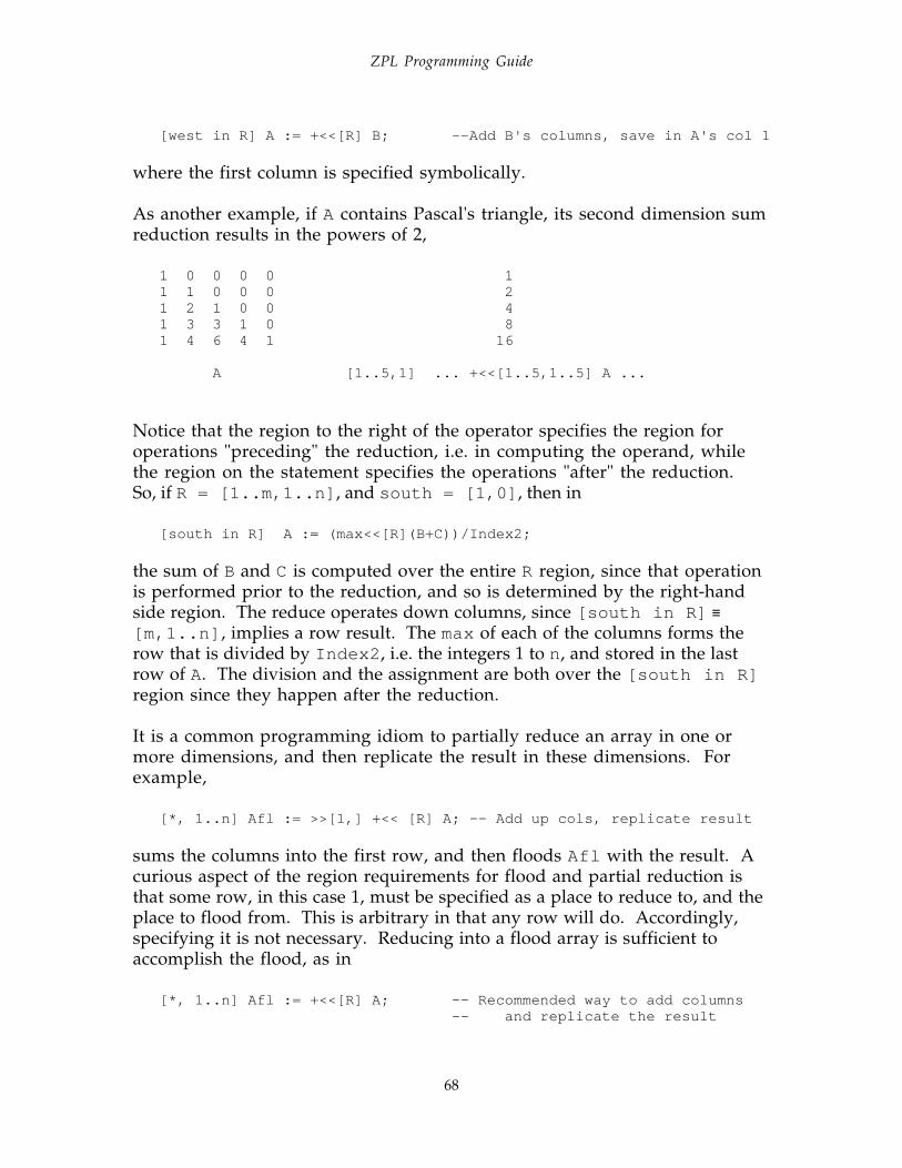
ZPL Programming Guide
68
[west in R] A := +<<[R] B; --Add B's columns, save in A's col 1
where the first column is specified symbolically.
As another example, if A contains Pascal's triangle, its second dimension sumreduction results in the powers of 2,
1 0 0 0 0 11 1 0 0 0 21 2 1 0 0 41 3 3 1 0 81 4 6 4 1 16
A [1..5,1] ... +<<[1..5,1..5] A ...
Notice that the region to the right of the operator specifies the region foroperations "preceding" the reduction, i.e. in computing the operand, whilethe region on the statement specifies the operations "after" the reduction.So, if R = [1..m,1..n] , and south = [1,0] , then in
[south in R] A := (max<<[R](B+C))/Index2;
the sum of B and C is computed over the entire R region, since that operationis performed prior to the reduction, and so is determined by the right-handside region. The reduce operates down columns, since [south in R] ≡[m,1..n] , implies a row result. The max of each of the columns forms therow that is divided by Index2 , i.e. the integers 1 to n, and stored in the lastrow of A. The division and the assignment are both over the [south in R]region since they happen after the reduction.
It is a common programming idiom to partially reduce an array in one ormore dimensions, and then replicate the result in these dimensions. Forexample,
[*, 1..n] Afl := >>[1,] +<< [R] A; -- Add up cols, replicate result
sums the columns into the first row, and then floods Afl with the result. Acurious aspect of the region requirements for flood and partial reduction isthat some row, in this case 1, must be specified as a place to reduce to, and theplace to flood from. This is arbitrary in that any row will do. Accordingly,specifying it is not necessary. Reducing into a flood array is sufficient toaccomplish the flood, as in
[*, 1..n] Afl := +<<[R] A; -- Recommended way to add columns-- and replicate the result
ZPL Programming Guide
69
which is conceptually cleaner, and is recommended.
Notice two points. First, although partial reduce and partial scan are related,the dimension over which the operation is performed is expressed differently-- for scan it is given in brackets, while for reduce it is given by the "change"in the region between the operand and result.
[1..n, 1] ... +<<[R] A ... -- Sum reduce rows [R] ... +||[2] A ... -- Sum scan rows
This difference is a consequence of the fact that the reduce must specify tworegions, while only one is needed for the scan. Second, neither operationchanges the rank of the operand, i.e. the result has the same rank as theoperand. So, in this example when the rows are summed up, the result isdefined over a column region, i.e. a rank 2 region, as shown on thestatement's region. This property motivates the topic of the next section.
As a closing observation, notice that there is a heuristic for remembering theoperators reduce, scan and flood. In reduce (<<), the result is "smaller" thanthe operand, in scan (||) the result is the same size as the operand, and inflood (>>), the result is "larger" than the operand. In addition, scan issometimes known as "parallel prefix."
Region Conformance
ZPL's operators have the property that their operands must be of the samerank, so that the selected values come from the same index set, possiblymodified by an @. Thus, if A and B are declared over R = [1..n,1..n] , theni n
[R] ... A + B ...
the addition refers to those elements of A and B with like indices from R. Thisis a strict rule. Thus, for example, if C is a rank three array declared over[1..c,1..n,1..n] , it might seem reasonable to write
[R][4,1..n,1..n] ... A + C ... -- ILLEGAL mixing of ranks
but the application of binary operators to operands of different rank is notpermitted.
A feature called rank change is planned for Advanced ZPL, which allows therank of arrays to be changed to accommodate situations like the one justillustrated. However, even when the capability is available, programmerswill achieve the best performance when they "work within the rank." This isbecause arrays are stored based on their ranks, and computing on operands of

ZPL Programming Guide
70
like rank assures that logically related values will be stored near one another,promoting efficiency. As will be seen, accommodating this requirement isnot onerous.
The situations where "working within a rank" become relevant typicallyinvolve flooding, partial reductions, and, since they are often used to select alower rank array, dynamic regions. Partial reductions provide a goodexample. Consider a 2D array A that is updated by some computation, and forwhich at the end of the iteration, the largest value in each row is compared tothe largest on the last iteration. This computation is given by
[1..n, 1] BigNew := max<<[R] A; -- Find largest in each row[1..n, 1] Ratio := BigNew/BigOld; -- Trend? >1 ==> increas'n
BigNew , BigOld and Ratio are logically one dimensional, but have beendeclared (elsewhere) to be "collapsed" 2D arrays, i.e. columns. This is becausethe partial reduce produces a single column result, determining BigNew . The"like rank" rule then forces BigOld and Ratio to conform.
Procedures
ZPL provides the usual procedure mechanism, including recursion. As withother languages, procedures in ZPL are a powerful structuring mechanismmaking a program easier to write, understand and maintain. But, proceduresare also a convenient mechanism for specifying concurrency through the useof promotion. This section covers procedure declarations, prototypes, calls,promotion and recursion.
Procedure DeclarationsProcedures are declared anywhere after the program statement, though it isconventional to declare them following the config var , constant ,direction , region , type and var declarations, since these are typicallyglobal information applicable to all procedures, implying they should bespecified first. The general form of a procedure declaration is
procedure PName ({ Formals}) {: Type}{ Locals}Statement;
where the non-italicized items must be given literally, the italicized itemsmust be replaced with text of the indicated type, and the items in braces areoptional. PName is a user specified procedure identifier. Type gives the typeof the procedure's result, i.e. the type of the value return ed for functions.Locals is an optional set of local-to-the-procedure variable declarations,which come into existence when the procedure is entered and are discarded

ZPL Programming Guide
71
when the procedure is exited. Statement is a single statement performing thecomputation, called the procedure body. This is usually, but not always, abegin -end compound statement. For example, an exceptional case would be
procedure absolute(x: float) : float;if x ≥ 0.0 then return x else return -xend;
a value returning procedure, i.e. a function, computing the absolute value ofits argument. Since the if -statement is a single statement, no begin -end isrequired to enclose it.
The (possibly empty) Formals list gives the procedure's formal parameters,separated by semicolons, i.e. the names of the arguments to be used in theprocedure's definition.* A single list item typically declares a sequence ofparameters of a single type according to the following scheme:
{ var } Id_List : Type
where the non-italicized items must be given literally, the italicized itemsmust be replaced with text of the indicated type, and the braces indicate anoptional item. The Id_List is a subsequence of the procedure's parameters, allof the same Type. For example,
procedure squarefloor( x, y : float; var xf, yf : integer);begin xf := floor (x * x); yf := floor (y * y);end;
has four parameters, two of which are float s, and two of which areinteger s. Further, the last two parameters are "by-reference" parameters,discussed momentarily.
If a formal parameter is an array, its characteristics must also be specifiedanalogously to its original declaration, as in
procedure even_up ( Odds : [R] integer) : [R] integer;return Odds - Odds % 2;
Such a specification requires that the arrays passed to the procedure bedeclared over R, but it does not require the computation be performed over allof R. Rather, the region over which the computation is performed will be
* Notice that the required parentheses explain why the program procedure, i.e. the procedurewith the program's name which typically has no arguments, is always specified with emptyparentheses.

ZPL Programming Guide
72
inherited from the call site, because no region specifier is given in theprocedure. Thus, for example, the procedure Compress0s , to shift a row of anarray left z positions,
procedure Compress0s( var z : integer; var Row : [R] float);while z > 0 do begin
Row := Row@east;z := z-1;
end;
has no region specifier in it. So, when it is called in a loop,
for i := 1 to m do j := amt; -- The amt of shift is j
[i, 1..n] Compress0s(j, A); -- Shift row i of A by jend
the region specifying the row to be shifted is inherited from the site of the call.That is, on the ith call to Compress0s , the region applying to the statementRow := Row@east will be [i, 1..n] .
Another way for a procedure to accept arrays as parameters is by the rankdefined mechanism. A rank defined specification gives only brackets andpossibly commas. These imply the argument's structure and allow theflexibility of arguments defined over different regions. Thus for example,
procedure Twice (X : [,] float) : [,] float;return 2.0 * X;
the X array is rank defined. All arguments passed to Twice must be rank 2,and their dimensions will be inherited. The applicable region will bewhatever the applicable rank 2 region is at the call site. Thus, in
[1..2, 1..2] A := Twice(B);
a 2 × 2 region of B is doubled, while in
[1..n,1] A := Twice(B);
the first column is doubled.
The rank of the parameter must be inferable from the rank of the arrayspecification. This is trivial when the region is given literally,
procedure P0(X : [R] float); -- X is a parallel array over region R
and straightforward for rank defined arrays.

ZPL Programming Guide
73
procedure P1(X : [,] float); -- X is a parallel array of rank 2 that -- inherits its region specification -- from the call site
It is not possible to infer the rank from a ditto specification, however, sincethe procedure might be called from sites where different ranks prevail. So,
procedure P2(X: ["] float); -- ILLEGAL use of ditto
is illegal. Finally, passing an indexed array
procedure P3(X : array[1..n] of float); -- X is an Indexed array
requires the array declaration to be given explicitly in the procedurespecification.
Parameters can be passed to a procedure by either of two methods, as by-valueparameters or as by-reference parameters. The procedure header indicateswhich form is being used: The keyword var indicates that the namesfollowing are by-reference parameters; otherwise, they are by-valueparameters. As a heuristic var means that the procedure can only be calledwith var iables in corresponding parameter positions.
In the case of value parameters the actual parameter's value (from theprocedure call site) is copied "into" the formal parameter variable of theprocedure. All references to this parameter within the procedure refer to thelocal copy. Modifications to by-value parameters change only the local copy.When the procedure exits, the copy is discarded. Consequently, anyassignments to the local copy will be lost.
For by-reference parameters, i.e. var parameters, no copy is made. Rather, allreferences to the formal parameter within the procedure simply refer to thevariable that is the actual parameter value from the call. Modifications to theformal parameter will change the actual parameter. Thus, by-referenceparameters are a secondary means of returning results to the caller, as shownin the squarefloor procedure above. The main purpose of by-referenceparameters is to save copying large parameters such as arrays and largerecords into the procedure. Wherever possible, var parameters should beused for this benefit.
Procedure PrototypesIt is essential that a procedure be declared before it is used. But, if inprocedure P there is a call to procedure Q, and within procedure Q there is acall to P, how can the declare-before-use rule be respected? The solution isthe procedure prototype, which is simply a completely specified procedure

ZPL Programming Guide
74
header in which the keyword prototype replaces the keyword procedure .For example,
prototype absolute(x: float) : float;
is a prototype for the absolute procedure from above. Notice that allinformation about the parameter types and return value are given as in thedeclaration. The prototype simply "stands in" for the declaration prior to theactual declaration. Thus, the sequence
prototype Q ( var x, y : float): float; -- State basics of Q's callprocedure P ( var u, v : float); -- Declare procedure P
. . .procedure Q ( var x, y : float): float; -- Declare procedure Q
. . .
gives a prototype for procedure Q so that it can be called (in procedure P) priorto its declaration. All parts of the procedure header must be given in bothplaces and be identical.
Procedure CallA procedure is called, or invoked, by giving its name and supplying theparameters. If the procedure is a value returning procedure then it may beinvoked in an expression as if it were an identifier. Thus
change := change + absolute(segment); --Accumulate magnitude
invokes the absolute procedure declared above. If the procedure is notvalue returning, it is invoked as a statement and must appear alone, followedby a semicolon. Thus, the squarefloor procedure, given above, is treated asa statement
squarefloor(xbase+deltax, ybase+deltay, xlimit, ylimit);
since it is not value returning, i.e. it returns its results by changing its last twoparameters. Notice that the (actual) parameters supplied in the procedurecall can be variables or expressions if the corresponding parameter is declaredas a by-value parameter. But if the parameter is declared as a by-referenceparameter using var , then the actual parameters in the call can only bevariables. Thus, in the squarefloor procedure call just illustrated,expressions can be used in the first two parameter positions only.
PromotionSequential procedures are procedures that use no array constructs, i.e. do notcontain parallel array declarations, region specifiers, uses of parallel arrays,wrap , reflect , flooding, mask, reduce or scan. They also cannot call non-sequential procedures. The absolute and squarefloor procedures defined

ZPL Programming Guide
75
above are sequential procedures. Sequential procedures can be promoted toapply to arrays. That is, their scalar (formal) parameters can be bound to array(actual) parameters in a call, to give the effect of applying the procedure toeach item of the arrays. For example,
[R] A := absolute(A); -- Remove negatives
applies the sequential procedure to items of the array A over the region R.
Promotion of sequential procedures is a convenient (and an efficient) way toperform complex operations in parallel on arrays. See Chapter 9 forexamples.
RecursionA procedure that calls itself, or calls a procedure sequence that ultimatelyresults in a call to itself, is said to be recursive. ZPL procedures can berecursive.
Procedure Declaration and Call Check List
A parameter's type must be declared, as well as the ranks of any arrays.Value parameters keep a local-to-the-procedure copy.With no local copy, by-reference parameters, i.e. var parameters, refer
indirectly to the actual parameters.Any changes in a procedure to value parameters are lost on exit.Any changes in a procedure to reference parameters persist on exit.Value parameters can be passed as an identifier or an expression.Only identifiers can be passed as by-reference parameters.
Figure 5.3 Procedure Usage Check List
Shattered Control-flow
ZPL programs that use scalars in control-flow expressions, such as
if n%2 = 0 then -- Check if problem size is even...
have a single, sequential thread of control, i.e. one statement is executed at atime. Specifically, in the statement forms
if lexpression then statements { else statements } end;
if lexpression then statements

ZPL Programming Guide
76
{{elsif lexpression then statements}}
{else statements} end;
for var := low to high { by step } do statements end;
while lexpression do statements end;
repeat statements until lexpression;
when the lexpressions, var, low, high and step are scalar values, there is onlyone statement executing at any time.
It is permissible to use parallel arrays in the lexpressions, var, low, high andstep positions of these control-flow expressions, subject to certain restrictions.Parallel arrays used for any of these values are said to cause the control-flowto shatter. In shattered control-flow, each index value has its own thread ofcontrol. When the statement list execution is completed, the control-flowreturns to sequential execution. The limitations are as follows:
Restrictions on shattered control-flow: The statement list formingstatements cannot assign to scalar variables. A variable modified by @must be identical in all instances. Uses of wrap , reflect , flooding,permutation, reduction, scan, mask and region specifiers are prohibited.
The restrictions ensure that when the control-flow shatters, the computationperformed at each index value is based on values that are "known" to thatindex. The intuition behind the restriction is that when the control-flowshatters, there is no guarantee what computation is taking place at otherindex positions, and so operations that reference other index positions, e.g.wrapping, may not be meaningful.
Though shattered control-flow may seem curious, it simply allows operationsto be written in the body of the program that could be realized by writing ascalar function and promoting it. For example, to compute factorial of eachelement of an array without shattered control flow, a scalar factorialprocedure would be defined,
procedure fact(n: integer): integer;begin var product, i: integer; product := 1; for i := 2 to n do
product := product*i;end;
return product;end;
and then applied to a (parallel) array of non-negative integers by promotion,
A := fact(B);

ZPL Programming Guide
77
to realize the result.
With shattering the factorial computation can be realized by the code,
A := 1; -- Initialize, so 0! is 1 and 1! is 1for I := 2 to B do
A := A*I; -- Compute the factorial of Bend;
assuming that I is declared as an array. The index variable of the for -loop isthe array I , and the loop limit is the array B. This is more direct and moresuccinct than the promoted function solution.
It is generally believed that using procedures is a good programmingtechnique, since they promote code reuse, encapsulate common processinglogic, promote abstraction, etc. But writing procedures for operations just forpromotion when they could easily be placed in-line in the program causesunnecessary proliferation of procedures. Shattered control-flow allows for in-line program text to behave like the application of a promoted scalarprocedure. Notice that if the factorial computation were required multipletimes in a program, the explicit use of a promoted function would become thepreferred solution, since it is about as efficient, names the operation andreduces the chance of making a notational error in writing the code.
The most common application of shattering is to perform differentcomputations on different array elements based on an if test. Thus,
if A >= 0 then B := sqrt(A); else B := sqrt(-A);end;
which is an effective way to realize selective execution. Masks are anotheralternative.
Masks
ZPL makes it trivial to operate uniformly on all elements of arrays, and it isnearly as simple to operate selectively on arbitrary subsets of regions. Themechanism is called a mask, and it is expressed as a modifier in a regionspecifier. Thus, in the sequence
M := A > 0; -- Boolean array, 1's at pos. positions[R with M] B:= sqrt(A); -- Take square roots of positive items

ZPL Programming Guide
78
M is an array of 1s and 0s indicating the truth value of the test. In the secondline, M is used as a mask. It specifies that the statement is to be applied only tothose indices of the region where M is nonzero, i.e. logically true. The formsof masking are,
[ R with M][ R without M]
where R is any region specifier including ditto, and M is a boolean , ubyte orsbyte . The without operator is the opposite of with , i.e. the statement isapplied to index values corresponding to zero's, i.e. logical false.
Masking, like all region specifiers used with statements, are scoped. Thus, amask applies to all of the statements within its scope. When masks arecascaded, i.e. a masked statement appears in a sequence of statements alreadymasked, the inner mask supersedes the outer mask(s). Thus, if
M1 ≡ 1 0 1 0 1 0 and M2 ≡ 1 1 1 0 0 0
then
[V] X := 1; -- X ≡ 1 1 1 1 1 1[V with M1] begin
X:=X+1; -- X ≡ 2 1 2 1 2 1 [V with M2] X:=0; -- X ≡ 0 0 0 1 2 1[V without M2] X:=4; -- X ≡ 0 0 0 4 4 4
end;
has the affect of applying operations within the begin-end compoundstatement to the odd index positions. Within the compound statement, thatapplication is superseded by M2 and its complement.
Finally, a mask can be changed within the scope in which it is applicable, butthe change is not manifest until after the completion of execution of thescope. Thus, in
[" with M1] begin S1; M1 := M1@west;
S3; end;
the changes to M1 will not apply until the next execution of the begin-endstatement.
Though the restrictions on shattered control-flow prohibit the use of masks,these can generally be performed prior to the shattering. For example,

ZPL Programming Guide
79
A := 1; -- InitializeM := B >= 0; -- Find nonnegatives
[R with M] for I := 2 to B do -- Mask outside the loopA := A*I; -- Factorial
end;
computes the factorial on only nonnegative values using masking. Since themask is applied to the statement, rather than to a statement in the body of theshattered loop, it is legal.

ZPL Programming Guide
80
-- Chapter 6 --
Programming Techniques
The power of ZPL derives largely from the fact that computations areexpressed by manipulating whole arrays rather than by manipulatingindividual scalar values, as in Fortran or C. There are several advantages:The programming is simpler when less detail is required, making theprogram easier to write in the first place and easier to understand later whenit must be changed. Also, arrays in ZPL express the computation in a simple,succinct way that is more likely to be analyzed successfully by the compilerthan is intricate scalar logic. When the compiler "understands" the program,it can produce highly efficient code customized to the target computer. Thus,the computations can actually be more efficient when expressed as arrays.
Though the examples in previous chapters have all been quite natural andobvious, programming with arrays may be sufficiently new to manyprogrammers that a discussion of principles and further illustrations of"standard" array techniques should be useful. Accordingly, this chapterworks through a series of computations solved using whole arrays:
Computation Constructs IllustratedMatrix Multiplication
Cannon's Algorithm Wrapping, dynamic regionsSUMMA Flooding
Sparse Matrix Product Indexed arraysRanking Partial reductionsHistogramming, revisited Flooding, Partial reductionsVector Quantization Data Compression Indexed arraysOdd/Even Transposition Sort Masking
The emphasis will be on using the new techniques introduced in the lastchapter, and illustrating good style. (To reduce detail, the "whole program"aspects of the examples such as including I/O will be dispensed with, sincethese are illustrated in Chapter 4.)
Matrix Multiplication
As mentioned in Chapter 1, finding the product of an m×n matrix A and ann×p matrix B producing an m×p matrix C is usually written in a scalarlanguage as a triply nested loop:

ZPL Programming Guide
81
FORTRAN MM C MM
DO 10 J = 1,M for (i=0;i<m;i++){ DO 10 I = 1,P for (j=0;j<p;j++){ C(I,J) = 0 c[i][j]=0; DO 10 K = 1,N for (k=0;k<n;k++){
10 C(I,J)=C(I,J)+A(I,K)*B(K,J) c[i][j]=c[i][j] +a[i][k]*b[k][j];
} }}
This specification is too rigid for effective use on high performancecomputers, since it specifies how to produce the result in a strict one-operation-at-a-time order. It states that c1,1 is to be produced before c1,2, andthat in producing each ci,j, the product ai,1b1,j is to be produced before ai,2b2,j,which in turn is to be computed before ai,3b3,j, etc. But, it is not necessary tofollow this rigid order to produce the result. All of the ci,j values can becomputed independently in any order or in parallel, all of the ai,kbk,jmultiplications of each dot product could be computed simultaneously, andeven the addition of these k subproducts to form ci,j can be performed withconsiderable concurrency. Some compilers attempt to figure out that suchrigid sequencing is not strictly necessary, and since matrix multiplication is anintensively studied example, they are frequently, but not always successful onthis computation [Ngo 97]. In general, however, computations are muchmore complex, compilers fail to eliminate the unnecessary sequentiality, andthe resulting object programs have very limited concurrency. Thus, when acomputation does not require a specific order of execution, it is preferable notto specify one. This is the concept behind ZPL's array operations. Thecompiler is more likely to produce efficient object code when irrelevantconstraints are not imposed by the programmer.
From these considerations a guideline emerges for formulating effectivealgorithms for ZPL programs. Since the operations in each statement of a ZPLprogram apply independently to all indices of the region, a useful rule is:
Maximize the size of the regions over which each statement applies.
This will result in a maximum number of independent operations for whichthe compiler can plan fast execution. Even when a ZPL program is notexecuted on a parallel machine, the rule will often aid the compiler inimproving performance of the cache, instruction pipeline, etc. A corollary tothe rule is suggested by previous discussions:
Minimize the use of intricate control-flow.
Since the control-flow enforces a specific order of execution, the moreinvolved it becomes, the less likely it is that a compiler will be successful in

ZPL Programming Guide
82
finding optimizations. Of course, both guidelines must be applied withjudgment.
How should matrix product be expressed in accordance with these guidelines?There are several ways to compute matrix product in ZPL, and two areconsidered here to illustrate computational ideas that are further discussedlater.
c11 c12 c13 a11 a12 a13 a14c21 c22 c23 ⇐ a21 a22 a23 a24c31 c32 c33 a31 a32 a33 a34c41 c42 c43 a41 a42 a43 a44
⇑
b13 b12 b23b11 b22 b33b21 b32 b43b31 b42b41
Figure 6.1. Cannon's matrix product.
Cannon's Algorithm: A well known approach that leads to a clean ZPLsolution is Cannon's algorithm [Cannon 69, Kung & Leiserson 80]. Toexplain the approach, visualize the computation (Figure 6.1) as taking place inspace. The result matrix C, initialized to 0.0, remains in a fixed position whileskewed instances of the A and B matrices are logically "passed over" C at rightangles. As elements of A and B "pass over" a result position, they aremultiplied together and added into that result position. Thus, on the firststep the value a4,1b1,3 is added to c4,3. On the second step both arrays advanceso that a4,2b2,3 is added into c4,3; additionally, a3,1b1,3 is added into c3,3, anda4,1b1,2 is added into c4,2. And so forth. The process completes when the Aand B matrices have completely passed over C.
At the mid-point in the computation multiplication and addition operationsare taking place at every position in the result array, a property that isconsistent with globally maximizing the independent operations. Towardsimproving the concurrency of the earlier and later steps, where not allpositions are participating, notice that the matrices can be given in a morenormal rectangular orientation by wrapping the skewed portions from thefront of the representation to the back in the case of A and from the top to thebottom for B. See Figure 6.2.
The lines show the boundary between the end of the skewed array and the"wrapped" portion. The principal effect of removing the skewing is that forthe computation to be correct, the two operand arrays must begin in asuperimposed position "above" C, and as the computation proceeds, their

ZPL Programming Guide
83
values must circulate by wrapping around in the direction of the arrows sothat the operand pairs of the subcomputations align. For example, in the c3,3position a3,1 of the A matrix is multiplied by b1,3 in the B matrix on the firststep. See Figure 6.2. If A is shifted-and-wrapped left on each step, and B isshifted-and-wrapped up on each step, the property that subcomputations ofci,j are performed at the i,j position will hold.
c11 c12 c13 a11 a12 a13 a14 |c21 c22 c23 a22 a23 a24 |a21c31 c32 c33 a33 a34 |a31 a32c41 c42 c43 a44 |a41 a42 a43
⇐
b11 b22 b33b21 b32 b43 | ⇑b31 b42 |b13b41 |b12 b23
Figure 6.2. Packing the skewed arrays into rectangular formfor the revised algorithm.
The key feature of this reformulation is that at each step computation istaking place at all positions in the result array, i.e. over its whole region,which achieves the goal of maximizing the region over which thecomputation is performed. The entire ZPL program to implement theCannon matrix multiplication solution is shown in Figure 6.3.
The first step is to formulate the declarations, beginning with the appropriateregions
region Lop = [1..m, 1..n]; -- Left operand shape Rop = [1..n, 1..p]; -- Right operand shape Res = [1..m, 1..p]; -- Result shape
which would collapse to a single region if the matrices were square.Although the shifting will be left for A and up for B, it will be moreconvenient, as explained below, if the directions point in the direction fromwhich the operands will come.
direction right = [ 0, 1]; below = [ 1, 0];
The remaining declarations
var A: [Lop] float; -- Left operand matrixB: [Rop] float; -- Right operand matrixC: [Res] float; -- Result matrixi: integer; -- Iteration variable
define the variables of the computation.

ZPL Programming Guide
84
1 region Lop = [1..m, 1..n]; -- Left operand shape 2 Rop = [1..n, 1..p]; -- Right operand shape 3 Res = [1..m, 1..p]; -- Result shape 4 5 direction right = [ 0, 1]; below = [ 1, 0]; 6 7 var A: [Lop] float; -- Left operand matrix 8 B: [Rop] float; -- Right operand matrix 9 C: [Res] float; -- Result matrix10 i: integer; -- Iteration variable
. . .12 for i := 2 to m do -- Skew A13 [right of Lop] wrap A; -- Move 1st col beyond last14 [i..m, 1..n] A := A@right; -- Shift last i rows left15 end;1617 for i := 2 to p do -- Skew B18 [below of Rop] wrap B; -- Move 1st row below last19 [1..n, i..p] B := B@below; -- Shift last i cols up20 end;2122 [Res] C := 0.0; -- Initialize C2324 for i := 1 to n do -- For A&B's common dimension25 [Res] C := C + A*B ; -- Form product and accumulate26 [right of Lop] wrap A; -- Send first col right27 [Lop] A := A@right; -- Shift array left28 [below of Rop] wrap B; -- Send top row down29 [Rop] B := B@below; -- Shift array up30 end;
Figure 6.3. Cannon's Matrix Multiplication
The first step is to skew the arrays in place. No skewing is required for thefirst row of A. The second row of A needs to be shifted left and wrapped oneposition, the third row must be shifted and wrapped around two positions,etc. The skewing will be performed iteratively, such that on the ith step, rowsi+1 through m are wrapped and shifted one position. A dynamic regionlimits the shifting to rows i through m.
for i := 2 to m do -- Skew A[right of Lop] wrap A; -- Move 1st col beyond last [i..m, 1..n] A := A@right; -- Shift last i rows left
end;
The effect of the wrap statement is to copy into the column to the right ofthe Lop region of A, the column on the opposite side of the array, i.e. the firstcolumn. Then, when A is replaced with itself offset to the right , the result isto shift the array left. The results of the three iterations needed to skew A ofthe previous example are shown in Figure 6.4.

ZPL Programming Guide
85
a11 a12 a13 a14| - a11 a12 a13 a14|a11a21 a22 a23 a24| - a22 a23 a24 a21|a21a31 a32 a33 a34| - a32 a33 a34 a31|a31a41 a42 a43 a44| - a42 a43 a44 a41|a41 Initial i=2 step
a11 a12 a13 a14|a11 a11 a12 a13 a14|a11a22 a23 a24 a21|a22 a22 a23 a24 a21|a22a33 a34 a31 a32|a32 a33 a34 a31 a32|a33a43 a44 a41 a42|a42 a44 a41 a42 a43|a43
i=3 step i=4 step
Figure 6.4. Intermediate values at the bottom of the loop while skewing A.
The logic
for i := 2 to p do -- Skew B[below of Rop] wrap B; -- Move 1st row below last [1..n, i..p] B := B@below; -- Shift last i cols up end;
for skewing B vertically is analogous. The final preparatory step is toinitialize the result array C.
Now, for as many items as there are in the common dimension, i.e. n , A ismultiplied by B and accumulated into C over the [Res] region, and the entireoperand arrays are cyclically shifted one position on each iteration.
for i := 1 to n do -- For A&B's common dimension[Res] C := C + A*B; -- Form product and accumulate
[right of Lop] wrap A; -- Send first col right[Lop] A := A@right; -- Shift array left
[below of Rop] wrap B; -- Send top row down[Rop] B := B@below; -- Shift array up
end;
Notice that unlike the initial skewing of the operand arrays, the wrapping inthe main loop involves all elements of both operands.
One property of this solution is that it leaves the operand arrays in thecompact-skewed position. If they are required in their proper form later, theymust be "unskewed." If so, it is preferable to begin by copying the arrays totemporaries which are used in the computation. These can be discardedrather than unskewed when the computation is completed. Notice that the Carray is oriented in its proper position. Finally, this solution accumulates theresults in an order different than is given in the sequential algorithm shownat the start of this section. The solution is equivalent for real numbers, ofcourse, but not necessarily identical in the finite precision of floating pointcomputer arithmetic.

ZPL Programming Guide
86
SUMMA Algorithm: Another solution that is especially easy to program inZPL is the Scalable Universal Matrix Multiplication Algorithm of van deGeijn and Watts [96]. In ZPL this algorithm can exploit the power of floodingfor the data communication. The result is a highly efficient program. Tosimplify the presentation, assume m=n, i.e. the matrices are square.
To explain the SUMMA algorithm, recall that every item ci,j in the matrixproduct result is the sum of the products of row i of A times column j of B.The first of these terms is ai,1b1,j. The SUMMA solution computes all of thesefirst terms simultaneously. This can be accomplished by flooding the firstcolumn of A and the first row of B into flood arrays, and multiplyingcorresponding elements:
a11 a 11 a 11 a 11 b 11 b 12 b 13 b 14 a 11b11 a 11b12 a 11b13 a 11b14a21 a 21 a 21 a 21 b 11 b 12 b 13 b 14 a 21b11 a 21b12 a 21b13 a 21b14a31 a 31 a 31 a 31 x b 11 b 12 b 13 b 14 = a 31b11 a 31b12 a 31b13 a 31b14a41 a 41 a 41 a 41 b 11 b 12 b 13 b 14 a 41b11 a 41b12 a 41b13 a 41b14
Flood A's 1st column Flood B's 1st row Result elements accum'd into C
The second term can be computed analogously, by flooding the secondcolumn of A and the second row of B. The algorithm continues in thisfashion, so that on the kth iteration the kth term of the dot product iscomputed and accumulated into the result array, C.
Notice that although each item in the result is computed by combining an Arow times a B column, to compute all of the entries simultaneously, we floodan A column and a B row. This may seem backwards, but as one can readilyrecognize, it allows the "matching" index positions to align. The easilyspecified ZPL program for the SUMMA algorithm is shown in Figure 6.5.
1 region M = [1..n, 1..n]; -- Region for n x n dense matrix 2 Fc = [1..n, *]; -- Flood region for left operand 3 Fr = [*, 1..n]; -- Flood region for right operand 4 var A,B,C : [M] double; -- Operand and result matrices 5 Af : [Fc] double; -- Flood array for left operand 6 Bf : [Fr] double; -- Flood array for right operand 7 k : integer; -- Iteration index
. . . 9 [M] C := 0.0; -- Initialize10 for k := 1 to n do11 [Fc] Af := >>[1..n,k] A; -- Replicate kth column of A12 [Fr] Bf := >>[k,1..n] B; -- Replicate kth row of B13 [M] C := C + Af*Bf;-- Compute kth term in dot prod.14 end;
Figure 6.5. Flood-based matrix multiplication solution.

ZPL Programming Guide
87
The program begins by declaring the necessary regions, including floodregions (Lines 2-3), and the appropriate variables. After initializing the resultarray C (Line 9), an iteration proceeds to compute each term of the dot productby flooding columns of A into Af , flooding rows of B into Bf , and multiplyingand accumulating the intermediate products (Lines 11-13).
This program is about the simplest possible solution for multiplying densematrices in ZPL,* even simpler than the straightforward Cannon algorithm.This is a happy outcome, because these algorithms use techniques exploitedin the fastest parallel matrix multiplication algorithms running on presentday parallel computers. This suggests that a critical ZPL design goal -- that itsfacilities should tend naturally to lead programmers to effective solutions --has been achieved in this instance at least.
As a postscript to this exercise programmers are reminded that matrix productis a common and expensive operation. Accordingly, vendors generallysupply a matrix product subroutine that is customized to their hardware.Such routines will generally run faster than a program written in a high levellanguage, though the ZPL flooding solution has outperformed libraryroutines. The programs given here are convenient, and will suffice for allbut the most intensive applications of matrix product. For these extremecases a call to such a library routine is generally advised.
Sparse Matrix Product
The matrices that arise in many scientific computations have the propertythat they are sparse, i.e. only a few of the entries are nonzero. Representingsuch matrices as dense matrices with all of the zeroes given explicitly is verywasteful of both space and time. So, these matrices are generally representedin compact form where only the nonzero values are stored. A typical compactform would represent each row by pairs of values, the first item of which isthe column index for the nonzero matrix entry, and the second item is itsvalue. Thus, if row 50 had nonzeroes in columns 49, 50, 51 and 52 then
(49, 2.0) (50, 4.0) (51, 6.0) (52, 8.0)
would be its compact representation.
As an illustration of computing with compact representations, consider asparse matrix multiplication computation. To simplify matters for the
* Flooding can be used to replicate the 2D arrays A and B into 3D to be multiplied togetherelementwise. The result is produced with a partial sum-reduction. This 1-line matrixmultiply, though still time and space efficient, is not as space efficient as the row-columnversion presented here.

ZPL Programming Guide
88
moment, only the special case of tridiagonal matrices will be considered, thatis, matrices in which the nonzeroes of row i are in columns i-1, i and i+1.Since all of the nonzeroes are in regular positions, storing the columnnumbers with the values is unnecessary. The values are stored in a lineararray, where each entry is a triple representing a row, such that the i-1st itemis stored in the first position, followed by the ith and i+1st items. Accordingly,the array
1 21 2 3 2 3 4 3 4 5 4 5 6 5 6 7 6 7
would appear as
0 1 21 2 32 3 43 4 54 5 65 6 76 7 0
In order that the diagonal (ith) element always to be in the second position, itis necessary to begin the first row in the second position. As will be seen laterit is convenient if the first element is assigned 0. Similarly, padding the lastrow with a 0 will make the algorithm work out nicely.
This approach implies the following declarations
region R = [1..n];type cform = array [1..3] of float;var A, B, C : [R] cform;
for the compact form data representation. Notice the region is onedimensional.
To formulate the matrix multiplication algorithm, focus on the elements of,say, the 4th row. Of the items in the resulting matrix, C, only three entrieswill be nonzero, c4,3, c4,4 and c4,5, and of the terms in their defining equations,
. . .c43 ≡ a 41b13+a42b23+a43b33+a44b43+a45b53 +a 46b63+a47b73
c44 ≡ a 41b14+a42b24+a43b34+a44b44+a45b54+a46b64+a47b74
c45 ≡ a 41b15+a42b25+a43b35 + a44b45+a45b55+a46b65+a47b75. . .

ZPL Programming Guide
89
only the elements shown in bold are nonzero. This simplifies thecomputation. For example, given that all three arrays are represented in thesame compact form, it is necessary only to refer to values in the rows aboveand below a given row, e.g. to compute row 4, only rows 3 and 5 need bereferenced. This motivates the definition of two directions,
direction above = [-1]; below = [+1];
to allow the previous and next rows to be referenced.
The computation of the product is direct by generalizing the equations givenabove. The three values for a row, C[1] , C[2] and C[3] , are computedsimultaneously by the equations
C[1] := A[1]*B[2]@above + A[2]*B[1]; -- i-1C[2] := A[1]*B[3]@above + A[2]*B[2] + A[3]*B[1]@below; -- iC[3] := A[2]*B[3] + A[3]*B[2]@below; -- i+1
Recalling that the indexes 1, 2 and 3 correspond to column indices i-1, i andi+1, the value of the diagonal element C[2] is computed by multiplying thethree values stored in an A row times the three B values found by selectingthe last value from the row above , the diagonal of the present row and thefirst value in the row below . The other two elements are similarlycomputed.
1 region R = [1..n]; -- Only 1D Region needed 2 type cform = array [1..3] of float; -- Create compact form 3 var A, B, C : [R] cform; -- Matrices are compact 4 direction above = [-1]; below = [+1]; -- Refer as rows
... 6 [R] begin 7 [above of R] B[] := 0.0; -- Initialize 0th row 8 [below of R] B[] := 0.0; -- Initialize n+1st row 9 C[1] := A[1]*B[2]@above + A[2]*B[1];10 C[2] := A[1]*B[3]@above + A[2]*B[2] + A[3]*B[1]@below;11 C[3] := A[2]*B[3] + A[3]*B[2]@below;12 end;
Figure 6.6. Tridiagonal matrix multiplication using compact form.
The three statements compute all elements of the result matrixsimultaneously, provided there is suitable initialization: First, the 0th andn+1st rows of B must be initialized to 0.0 so that the above and belowreferences are defined and vanish when computing the terms for the first andlast rows, respectively. This motivates the initialization
[above of R] B[] := 0.0;[below of R] B[] := 0.0;

ZPL Programming Guide
90
By leaving the brackets empty, the assignment is to each element of the triple.Second, to assure that the C[1] entry for row 1 and the C[3] entry for row ncompute to zero, B[1] of row 1 and B[3] of row n must be initialized to 0.0 aswell. Since this is the normal way to represent the array, the requirement istreated simply as a property of the input, rather than a value to be computed.The result is shown in Figure 6.6.
Ranking
Ranking a set of items is a common operation. It is easily performed in ZPL.For the example here, assume that the n items to be ranked come from somesmall finite set of values such as the integers 1 to s. There will be duplicates,since s << n, and the rule is that when values are the same, the one with thelower index in the input is to have the lower rank.
Input (s=3): 3 1 1 2 1 3 Output: 5 1 2 4 3 6
3 1 1 2 1 3 1 1 1 1 1 1 0 1 1 0 1 0 0 1 2 2 3 3 0 1 2 0 3 0 5 1 2 4 3 63 1 1 2 1 3 2 2 2 2 2 2 0 0 0 1 0 0 3 3 3 4 4 4 0 0 0 4 0 03 1 1 2 1 3 3 3 3 3 3 3 1 0 0 0 0 1 5 5 5 5 5 6 5 0 0 0 0 6Flood Input Index1 P +||P P*(+||P) Reduce Cols
Figure 6.7. Ranking n=6 items ranging over s=3 values.
The technique is to use an s × n temporary array P to represent the position ofthe item. See Figure 6.7. P is set to 0's and 1's such that there is a 1 in positioni,j if item j has value i; and 0's elsewhere. These settings are computed byflooding the input into the rows of an array and comparing that to the rowindex, Index1 . By adding up these 1's (with a scan) and removing theintermediates (by multiplying by P), the columns of P can be reduced to yieldthe result. A program fragment is shown in Figure 6.8.
1 region Io = [1, 1..n]; -- Region for the input/output 2 R = [1..s, 1..n]; -- Basic working region 3 F = [*, 1..n]; -- Flood region 4 var In,Out : [Io] ubyte; -- Problem is limited to 256 < s 5 P : [R]; -- Processing array 6 Z : [F]; -- Flood array
. . . 8 [F] Z := >>[Io]In; -- Replicate the input 9 [R] P := Z = Index1; -- Mark where there are items?10 [R] P := P * (+||P); -- Find the overall order11 [Io] Out := +<<[R] P; -- Add up columns w/partial reduce
Figure 6.8. Ranking computation based on scan and partial reduction

ZPL Programming Guide
91
Several features of the program are significant. First, the source array (In )and output array (Out ), which are logically one dimensional arrays, aredefined to be single-row two dimensional arrays. This is because thecomputation will operate in two dimensions, and it is highly efficient to work"within the same rank," as explained in the discussion on RegionConformance in the last chapter.
Second, the computation relies on the fact that the plus-scan wraps aroundon each row as it accumulates the entries of an array.
Third, the partial reduce that adds up the columns must specify whichdimension is being reduced. This is expressed by the "difference" between theregion of the statement [Io] and the region following the operator [R] .Specifically, the region on line 11 is [1,1..n] , while the region specified withthe reduction is [1..s,1..n] , implying that the first dimension reduces.
Finally, the computation may appear very "heavy weight," but in fact it islikely to be quite efficient. As mentioned in the flooding definition, floodarrays are represented with only the defining values. So, Z is not 2D despitebeing used that way. Index1 is a logical array created by the compiler, anddoes not occupy memory. The scan operation will be implemented by theefficient parallel prefix technique, as will the reduction. Finally, though ZPLrelies on the native C compiler for low level optimizations, many compilersperform "strength reduction" optimizations on operations such as themultiply by 0-1 values here, i.e. an equivalent sequence of operations notinvolving multiply may be used. And even when the compiler doesn'tperform strength reduction, it is likely that the multiply is a better choice thanan if-then-else on modern pipelined processors. Thus, this rankingsolution is likely to be reasonably efficient even ignoring the benefits ofparallel processing.
Histogramming, Revisited
In Chapter 4 a small histogramming program was presented, which printedthe ranges of the intervals and the number of items assigned to each interval.Using the ideas from the ranking example above, it is possible to consider analternative implementation based on the partial reduce operation. See Figure6.9.
This solution begins by revising the previous 1D region to a 2D, single rowregion. The logic follows the earlier solution, computing bin numbers bydividing each item by the interval size, correcting to 1-origin. Thehistogramming operation comes in the final line where the BinNo array isflooded in the first dimension, i.e. the rows are replicated, and then comparedto Index1 to create a logical array that is accumulated row-wise to form the

ZPL Programming Guide
92
result. The size of the flooded intermediate array comes from the regionspecified with the partial reduction, i.e. [1..b,1..n] . The partial reduce isperformed across the second dimension, as can be seen by inspecting theregion of the partial reduction operator and the region of the context (Line14).
Revisit the example from the Chapter 4 historgram program, in which b ≡ 3and the input
Values ≡ 6.3 -4.2 0.0 1.9 5.4 -2.2 -4.2 -2.2
resulted in bin numbers
BinNo ≡ 3 1 2 2 3 1 1 1
Then Line 14 produces the result 4 2 2 and the intermediate valuesshown in Figure 6.10.
This is effectively the same solution as presented before, except that it isperformed as a single operation rather than iteratively. And, like the rankingsolution, should be efficient for moderate values of b.
1 region Rw = [1,1..n]; -- The index space of the data 2 var small, big, size : float; -- Real scalars 3 Hist : [1..b,1] integer; -- Array to hold histogram 4 Values: [S] float; -- Data value array 5 BinNo : [S] ubyte; -- Interval no., expect at most 255
. . . 7 [S]begin 8 small := min<<Values; -- Find a smallest value 9 big := max<<Values; -- Find a largest value10 size := (big-small)/b; -- Figure size of the intervals11 BinNo := ceil((Values-small)/size);-- Compute position, round up12 BinNo := BinNo + !BinNo; --Include small endpoints in first13 -- bin yielding 1-origin indexing14 [1..b,1] Hist := +<<[1..b,1..n](Index1 = >>[1,1..n] BinNo);15 -- Flood BinNo down columns, compare16 -- to create logical rows to sum17 -- over to find histogram directly18 end;
Figure 6.9. Revised histogram computation.
1 1 1 1 1 1 1 1 3 1 2 2 3 1 1 1 0 1 0 0 0 1 1 1 42 2 2 2 2 2 2 2 3 1 2 2 3 1 1 1 0 0 1 1 0 0 0 0 23 3 3 3 3 3 3 3 3 1 2 2 3 1 1 1 1 0 0 0 1 0 0 0 2
(a) (b) (c) (d)
Figure 6.10. Values from Line 14 of the Histogram program of Figure 6.9 (a) Index1, (b) >>[1,1..n] BinNo, (c) Index1 = >>[1,1..n] BinNo, (d) Hist.
ZPL Programming Guide
93
Vector Quantization Data Compression
The bits of an image are often compressed so that, for example, they can betransmitted efficiently over a low bandwidth communication link. There arelossless compression schemes that allow all bits of the image to bereconstructed later, and lossy compression schemes that lose someinformation in order to achieve a much greater degree of compression. Lossyschemes are chosen when the use made of the images is not materiallyaffected by the lost information. Vector quantization is one such lossyscheme.
In vector quantization a codebook is created by "training" it on a sample set ofimages. This codebook is then used to compress/decompress the images. Inthe ZPL program shown here, the 8-bit pixels of an image are considered to bearranged in 2×2 groups which are matched against the 2×2 pixel entries of a256-entry codebook and replaced by the index of that codebook entry that mostclosely matches. Thus, this lossy scheme achieves a 4:1 compression ratio.The 2×2 groups motivate the definition of a data type, block , which is a 2×2indexed array. The images (Im ) and the codebook (CB) have blocks as items.The simple program is shown in Figure 6.11.
The program begins with the declarations, all of which are by now standard,except for the data type declaration block . The variable Im represents animage as block s, so that its default size in block s, 512 × 512, implies animage of 1024 × 1024 size in pixels.
A function dist(b1, b2) is defined to take two block s as parameters andreturn the floating point number that is the mean square distance betweenthem. Since the blocks are 2D indexed arrays, the computation simply makesexplicit reference to the items of the blocks, and returns the result. Theprocedure is a scalar procedure in the sense that it takes single items of typeblock as parameters, though these elements are themselves arrays, of course.When the dist procedure is used in the body of the program, it will be calledwith a scalar first argument, a block from the codebook, and an array secondargument, the image. This causes the procedure to be promoted to apply toeach position, i.e. each block of the image.
The program begins by reading in the codebook CB which, to avoid beingdistracted by the details of I/O, is not shown. Then, in the processing loopimages are read in, compressed, and the compressed results are written out.The logic of the processing loop is particularly simple. The "old" distancearray, Disto , is initialized to be the distance of every image block to the firstcodebook entry. Then, for the remaining entries in CB, the "new" distance toevery image block Distn is computed, and the best so far is stored in the

ZPL Programming Guide
94
Coding array. When all codebook entries have been considered, the contentsof Coding is the compressed image, which is written out.
1 config var n : integer = 512; -- Image size 2 region R = [1..n, 1..n]; -- Problem domain 3 type block = array [1..2, 1..2] of ubyte; 4 -- The compression is based on 5 -- 2x2 blocks of 8-bit pixels 6 var CB: array [0..255] of block; -- Codebook, an indexed array 7 Im: [R] block; -- Image array 8 Disto, -- Old distance array 9 Distn: [R] float; -- New distance array10 Coding: [R] ubyte; -- Coding array11 i: integer; -- Loop index1213 procedure dist(b1, b2: block): float;14 -- A function to compute the mean square distance15 -- Block b2 to be promoted16 return ( (b1[1,1] - b2[1,1])^217 + (b1[1,2] - b2[1,2])^218 + (b1[2,1] - b2[2,1])^219 + (b1[2,2] - b2[2,2])^2)/4.0;
. . .21 -- Input codebook here22 [R] repeat -- Compress all images ...23 -- Input an image blocked into Im24 Disto := dist(CB[0],Im); -- Init old distance array25 Coding := 0; -- 1 is closest so far2627 /* Move through codebook, finding how they match up */28 for i := 1 to 255 do29 Distn := dist(CB[i],Im); -- Compute distance for entry30 if Disto > Distn -- Shatter to process entries31 then32 Disto := Distn; -- New distance is smaller33 Coding := i; -- ith entry is best so far34 end;35 end;36 -- Output the compressed image in Coding37 until no_more;
Figure 6.11. Lossy data compression program.
Notice that the update of the best match (Lines 30-34) is performed usingshattered control flow. That is, the condition of the if -statement
Disto > Distn
is a test over arrays, so the statement is executed independently for everyindex in the region, R. For those in which the best previously computeddistance, Disto , is larger than the new distance, Distn , the new distance issaved and its index stored in Coding . For those indices for which thecondition does not hold, there is no change.

ZPL Programming Guide
95
The Compress computation is highly efficient. Since the codebook array, CB,is an indexed array it is replicated on each processor when the program isexecuted in parallel. This means that each processor of a parallel computercan perform its part of the compression without any interprocessorcommunication. This makes the core of the program maximally concurrent.The key issue in the program's performance concerns the details of reading inthe raw images and writing out compressed images. Parallel I/O is crucial,but unfortunately it is a very machine specific operation. So, it is not possibleto evaluate the performance of this computation fully.
Odd/Even Transposition Sort
Ordering a set of elements is a computation with wide application, and onethat has been intensively studied. Since it is generally possible to sort muchfaster when one exploits the specifics of a particular computer, vendorstypically provide a highly optimized sorting procedure customized to theirhardware. When the data set is very large, or sorting is used repeatedly, it isadvisable to invoke the library procedure, rather than a sort written in ZPL orany high level language. Nevertheless, sorting provides a handy illustrationof several language features.
The Odd/Even Transposition Sort orders a linear array of items by comparingeach odd indexed item with the next element, and interchanging them if theyare out of order. This operation applied to all odd-even pairs is called a halfstep, and clearly, since the data items do not interfere, the operations can beperformed simultaneously. The other half step is to perform the sameoperation on each even-odd pair. The sort repeatedly applies the two halfsteps until no interchanges take place, i.e. every element is in order withrespect to its successor.
A ZPL program for the masking version of the computation is shown inFigure 6.12. The program begins with standard declarations. It then sets up aconstant array, Oe, which has 1 's in alternating positions (Line 12). The logicof the program after initializations is to iterate (Lines 19-36), performing thetwo half steps until there is no change, i.e. unordered (Line 34) is false. If thearray is initially sorted, the loop is never entered, due to the initialassignment (Line 16) of unordered .
Of interest is the use of masking to restrict attention first to the out-of-orderodd-even pairs (Lines 22-25), and then the out-of-order even-odd pairs (Lines29-32). In Line 22, Mask is true for odd indexed values that are larger than thefollowing element, and it is only for these values that the array operationswithin the begin-end statement will have an effect. Accordingly, if Mask istrue for index i, the ith element of Temp is assigned the smaller value, and thei+1st element of Temp is assigned the larger value of the pair. Notice that each

ZPL Programming Guide
96
index value is considered for each statement, and so the execution time is notsignificantly affected by how many Mask bits are set.
1 program OET_Sort; -- Odd/Even Transposition Sort 2 3 config var n : integer = 100; -- Problem size 4 region V = [1..n]; -- Problem Space 5 direction next = [1]; -- Reference to right neighbor 6 7 procedure OET_Sort(); -- Entry point 8 var Val, Temp : [V] float; -- Value arrays 9 Mask, Oe : [V] ubyte; -- Arrays to mark interch's10 unordered : boolean; -- Termination condition11 [V] begin12 Oe := Index1%2; -- Set alternate positions13 read(Val); -- Get input14 [next of V] Val := max_float; -- Disable final element15 Mask := Val > Val@next; -- nonzeroes indicate disorder16 unordered := |<<Mask; -- Is there disorder?17 Temp := Val; -- Initialize1819 while unordered do20 /* Odd Halfstep */21 Mask := Mask & Oe; -- Mark odd unordered items22 [" with Mask] begin -- Wherever these occur23 Temp := Val@next; -- Set larger24 Temp@next := Val; -- Set smaller25 end;26 Val := Temp; -- Update27 /* Even Halfstep */28 Mask := (Val>Val@next) & !Oe;-- Consider evens29 [" with Mask] begin -- Wherever disorder exists30 Temp := Val@next; -- Set larger31 Temp@next := Val; -- Set smaller32 end;33 Mask := Val > Val@next;--Where disorder remains34 unordered := |<<Mask; -- Any change?35 Val := Temp; -- Update36 end;37 writeln(Val); -- Print it38 end;
Figure 6.12. Odd/even transposition sort.
To assist in understanding the execution of OET_Sort , these intermediatevalues of Mask and Val for n=8
Line 21.5 Line 28.5 Mask Val Mask Val .1 0 1 0 0 0 0 0 3 1 4 1 5 9 2 6 0 1 0 0 0 1 0 0 1 3 1 4 5 9 2 60 0 0 0 1 0 1 0 1 1 3 4 5 2 9 6 0 0 0 1 0 0 0 0 1 1 3 4 2 5 6 90 0 1 0 0 0 0 0 1 1 2 3 4 5 6 9 0 0 0 0 0 0 0 0 1 1 2 3 4 5 6 9

ZPL Programming Guide
97
were produced by inserting write statements before the masked compoundstatements, i.e. at Lines 21.5 and 28.5.
References
L. F. Cannon, 1969. "A Cellular Computer to Implement the (Kalman) FilterAlgorithm," PhD Thesis, Montana State University.
H. T. Kung and C. E. Leiserson, 1980. "Algorithms for VLSI Processor Arrays,"In Carver Mead and Lynn Conway, Introduction to VLSI Systems,Addison Wesley.
Ton Ahn Ngo, 1997, The Effectiveness of Two Data Parallel Languages, HPFand ZPL, PhD Dissertation, University of Washington.
Robert van de Geijn and JerrellWatts, 1997, "SUMMA: Scalable universalmatrix multiplication algorithm," Concurrency Practice andExperience, 9(4):255-274.

ZPL Programming Guide
98
-- Chapter 7 --
Advanced ZPL Concepts
In previous chapters fundamental ZPL concepts such as regions, directions,translations, etc. have been introduced. In this chapter, generalizations tothose concepts are introduced that allow much more sophisticated programs.
Strided Regions and Arrays
In addition to working with dense arrays, ZPL programmers also have theability to compute over arrays in which elements have been uniformly"removed." The regions and arrays are called strided, because skippingindices at regular intervals between referencing elements is suggestive of"walking" over the index ranges with "long strides." Strided arrays are theway in which multigrid and wavelet computations are expressed in ZPL.
As with other features of ZPL, striding is accomplished through the use ofregions. To "stride" a region, the key word by is used with a direction, as in
region S = [0..9, 0..9] by [ 2, 2];
which has the effect of defining S to have only even number indices in bothdimensions. That is, beginning with a region with 100 index pairs, thedefinition of S yields a region with only 25 index pairs.
S = {(0,0), (0,2), (0,4), ..., (2,0), (2,2), (2,4), ... , (8,8) }
In effect, the direction gives the stride for each dimension, i.e. the amount tobe added to an index in each dimension to find the next index.
Strided regions are usually defined from a base region. Thus,
region R = [0..n-1, 0..n-1];S = R by [ 2, 2];
defines R and then defines S as a strided by [2,2] variant of R. Notice thatthe index sets of R and S are related in that S contains alternate indexpositions of R. Of course, it is possible to make multiple regions, as in

ZPL Programming Guide
99
region R = [0..n-1, 0..n-1];S2 = R by [ 2, 2];S4 = R by [ 4, 4]; -- Recommended styleS8 = R by [ 8, 8];
which could also be defined successively, as in
region R = [0..n-1, 0..n-1];S2 = R by [ 2, 2];S4 = S2 by [ 2, 2]; -- Alternate formS8 = S4 by [ 2, 2];
In general, it is thought to be better programming style to define all stridesrelative to the base region, i.e. the first form is preferred. Some ZPLprogrammers find it convenient to use indices in the base range 0..n-1rather than the range 1..n in order to make it easy to express which items arepresent in a strided region, e.g. "indices divisible by 4".*
It is not necessary to stride in all dimensions. To declare a region with denseindices in the first dimension, but alternate indices in the second dimension,i.e. stride the rows, write
region Sr = R by [ 1, 2]; -- Stride rows by 2
Similarly, a three dimensional region with only the first dimension stridedmight be declared
region S3D = [0..r, 0..s, 0..t] by [2, 1, 1];
Of course, the stride amount must be a positive integral value. Notice theuseful heuristic that the direction gives the dimensions of the bounding boxof the subarray that is "collapsed" into each strided index.
Strided regions can be used wherever dense regions can be used. As withother region specifications it is possible to stride regions dynamically. Thus
[[0..i-1] by [2]] ...; -- Reference alternate elements up to i
defines a one dimensional dynamic strided region, where the value of i isbound when the statement is executed.
* Some multigrid programmers think of the indices of the coarser grids as dense, i.e. asstepping by a unit stride. ZPL does not provide the ability to remap strided indices into densesequences, preferring instead to preserve the correspondence between present elements of anystride. But, if 0-origin indexing is used, then it is easy to mentally remap the indices to densepositions, since strided region indices always have the stride as a factor, assisting mentalremapping. Thus, for example, index 12 would correspond to index 6 in a dense remapping of astrided-by-2 dimension, while it would correspond to index 3 for a dense of remapping of astrided-by-4 region.

ZPL Programming Guide
100
Arrays with strided indices are declared in the usual way using stridedregions. Thus, assuming the declarations given above,
var By2Pos: [S2] double; -- Strided array with even indices By4Pos: [S4] double; -- Strided array with indices div by 4 By8Pos: [S8] double; -- Strided array with indices div by 8
defines arrays with the index sets indicated.
Recall that in Chapter 3, the following rule was introduced:
Any array can be used in the scope of any region specifier provided thearray is defined for all indices specified in the region.
In Chapter 3 the rule prevented the use of arrays whose index sets weresmaller than the regions in whose scope they were used. In the context ofstrided arrays, the rule means that computations must be performed in thescope of region specifiers that are aligned and have the same or larger strides.Thus, assuming the declarations from above,
[S2] By2Pos := 0; -- Initialize strided region
is the proper way to reference a strided region, but
[R] By2Pos := 0; -- ILLEGAL
is illegal because R contains index pairs that By2Pos does not have. The ruleprohibits this kind of usage.
Of course, it is quite appropriate for an array to have more elements than arereferred to in the strided region. So, assuming the declarations
region R = [0..n-1, 0..n-1]; S2 = [R] by [2,2];var X : [R] double; Xby2 : [S2] double;
a possible way to aggregate the elements of X into Xby2 would be expressed
[S2] Xby2 := 0.4*X + 0.25*X@east + 0.25*X@south + 0.1*X@se;
where the region is strided, as is the left-hand side array, but the array, X, isdense. The elements of X that are referenced in the subexpression 0.4*X arethose of the region S2. The X@east expression in the scope of S2 means thatthe elements of X with an odd index in the second position are to bereferenced. That is, the direction east = [0,1] is added to each of theindices of the strided region as usual to produce a new index set with whichto reference X. Similarly for X@south and X@se. Of course, border regions

ZPL Programming Guide
101
may be required on the right and bottom to assure that all references aredefined, e.g. when n is odd.
As just discussed when the array is dense, directions define neighbors in theusual way even if the region providing the index set happens to be strided.When the array is strided, directions also define neighbors in the usual way,but now there is a subtlety. What is the east neighbor of a strided-by-2dimension? In the dense case the east neighbor can be computed by adding 1in that dimension, i.e. by adding the stride, and in the strided-by-2 case theeast neighbor is also found by adding 2, the stride.
Consider a strided-by-2 linear array Alt ,
var Alt : [0..n-1] by [2] double;
whose values are to be linearly interpolated to fill a dense array Full . Thedirection right2 = [2] is used to reference the next element in the stridedregion in the statement sequence
[[0..n-1] by right2] begin Full := Alt; -- Set evens Full@right := (Alt+Alt@right2)/2.0;--Set oddsend
where right = [1] refers to the next among the dense indices, and there isassumed to be a border element of Alt with index n.
An alternative way to have expressed the same computation would havebeen to refer to the two strided subsequences of [0..n] separately, and to useleft = [-1] to reference the previous element, as in
[[0..n-1] by right2] Full := Alt; -- Set evens[[1..n] by right2] Full := (Alt@left + Alt@right)/2.0;-- Set odds
Though Alt is not defined for any of the indices in [[1..n] by right2] ,the fact that each instance of Alt in the second line is modified by a directionthat produces only indices of defined values fulfills the requirements of thepreviously mentioned rule.
In summary, the neighboring elements of a strided array can be referred tousing @d, but it is essential that when direction d is added to the indices of theapplicable region that they refer to defined elements of the array. This willgenerally mean that the neighbor referenced with direction d in a dense arraywill have to be scaled by the stride to perform the same reference in thestrided array.

ZPL Programming Guide
102
Multidirections
Strided regions often present situations in which it is convenient to"compute" directions, i.e. the specific neighbor to be referenced is a variablerather than a constant. Much of the flexibility of fully computed directionscan be achieved by using multidirections.
A multidirection is a regular sequence of directions with a common name.The elements of the sequence can be referenced by name and index. Thegeneral form is to declare the multidirection as follows
direction Dname{ index set } = direction scaledby expression;
where
Dname is an identifier naming the directionindex set is a nonnegative lower and upper limit separated by ..direction is any direction, i.e. integer d-tupleexpression is any arithmetic expression containing instances of the
symbol {} in operand positions
and all other symbols must be given as shown. For example, assuming the1D direction right = [1] the multidirection declaration
direction stride_right {0..5} = right scaledby 2^{};
defines the sequence of six directions,
stride_right{0} ≡ [1] * 2^0 ≡ [1]stride_right{1} ≡ [1] * 2^1 ≡ [2]stride_right{2} ≡ [1] * 2^2 ≡ [4]stride_right{3} ≡ [1] * 2^3 ≡ [8]stride_right{4} ≡ [1] * 2^4 ≡ [16]stride_right{5} ≡ [1] * 2^5 ≡ [32]
of varying distances to the right. The multiple directions are defined relativeto a base direction, in this case right , by scaling with the expression. Thebrace pair {} stands for multidirection indices such that the ith index ireplaces the brace pair in the expression.
Like all directions multidirections are referenced using the standard @ symbolwith operands except that an index is also specified in braces, {} . Thus, forexample, assuming the stride_right directions declared above,
for i := 0 to 5 do

ZPL Programming Guide
103
... A@stride_right{i} ...end;
has the effect of referencing items of A shifted right one position for i = 0 ,then two positions for i = 1 , etc., up to 32 positions to the right for i = 5 .
In the multidirection declaration the lower and upper limits of the indexinterval are arbitrary expressions evaluating to nonnegative integer constants(lower ≤ upper). The base direction can be any legal direction. The scalingexpression can be any expression involving instances of a brace pair, {} inoperand positions and evaluating to an integer. For each index in the rangethe expression is evaluated with that index value substituted for alloccurrences of {} , and the result is multiplied times each dimension of thebase direction to yield the direction for that index.
As a further illustration, assuming se = [ 1, 1] , the
direction SE{1..4} = se scaledby {};
defines the four directions
SE{1} ≡ [1,1] * 1 ≡ [1,1]SE{2} ≡ [1,1] * 2 ≡ [2,2]SE{3} ≡ [1,1] * 3 ≡ [3,3]SE{4} ≡ [1,1] * 4 ≡ [4,4]
which point to the four consecutive elements below and to the right of agiven element. Another application for multidirections is restructuring adense array into a strided array of arrays. Given the declarations
region V = [0..3*n-1];var D : [V] float; -- Dense array of 3n items
S : [V by 3] array [0..2] of float;-- Sparse array of triplesdirection r{0..2} = [1] scaled by {}; -- Pt to self, next, next+1
the multidirection r is composed of the three directions [0] , [1] and [2] .Then, in the program
[V by 3] for i := 0 to 2 do S[i] := D@r{i}; -- Fill elements of Send;
the strided array S is loaded from D. (See Figure 7.1.) That is, the dynamicregion, with indices {0, 3, 6, ...} references all and only the items of S, and eachelement of S, a 3-element array, is loaded with the corresponding threesuccessive elements of D, as the figure illustrates. Such restructuring hasmany applications.

ZPL Programming Guide
104
S[0] S[3] S[6]
D
First Iteration: [R] S[0] := D@r{0}; -- Same S[0] := D
Figure 7.1: Loading sparse-indexed vector of triples fromdense array using a multidirection.
Multiregions and Arrays
Hierarchically structured data and algorithms are common in computing.For example, multigrids are formed from dense grids by striding at multiplelevels. Wavelets are another example. The number of levels is determinedby the size of the input, and therefore cannot be determined before programexecution time. Accordingly, the concept of a multiregion is essential fordefining and computing on an arbitrarily deep hierarchy.
In the same way that directions are extended to be indexable, so too, areregions. The general syntax for a multiregion is:
region Rname {} = region by direction{} ;
where
Rname is an identifier naming the regionregion is any dense regiondirection is any multidirection name followed by empty braces.
and all other symbols must be given as shown. That is, multiregions are thesame as other strided regions, except that the direction is a multidirection.For example,
direction sepow2{0..log2(n)} = [1,1] scaledby 2^{};-- By powers of 2
defines for n ≡ 16 the directions
sepow2{0} ≡ [ 1, 1]sepow2{1} ≡ [ 2, 2]sepow2{2} ≡ [ 4, 4]sepow2{3} ≡ [ 8, 8]sepow2{4} ≡ [16,16]

ZPL Programming Guide
105
The region specification
region H{} = [0..n-1, 0..n-1] by sepow{}; -- Hierarchical region
therefore, defines for n ≡ 16 a five level hierarchy
H{0} ≡ {(0,0), (0,1), (0,2), ..., (15,15) }H{1} ≡ {(0,0), (0,2), (0,4), ..., (14,14) }H{2} ≡ {(0,0), (0,4), (0,8), ..., (12,12) }H{3} ≡ {(0,0), (0,8), (8,0), ( 8, 8) }H{4} ≡ {(0,0) }
in which the 0th level is a 16x16 dense region, the 1st level is an 8x8 regionstrided by [2,2] , the 2nd level is a 4x4 region strided by [4,4] , the 3rd is a 2x2region strided by [8,8] , and the 4th is a 1x1 region with a single index value.Clearly, when n ≡ 64 the R region is a seven level hierarchy, etc.
As suggested in the example, multiregions are referred to by appending abrace pair containing the index of the level being referenced. For example,
[H{3}] X := Y; -- Update X
has the effect of updating four elements of X, assuming the declaration above.In general, an indexed multiregion can be used wherever standard regionscan be used.
Since regions are used to declare arrays, it follows that declaring an array witha multiregion must produce a multiarray. Multiarrays are declared using amultiregion with empty braces with the region specifier, as in
var G{} : [H{}] double; -- Declare multiarray G
and they are referenced by appending braces with an index, as in G{1} . Thesemantics simply extend the normal meaning of array. That is, the identifier,G in this case, refers to an array with index positions corresponding to eachindex in the multiregion. This can be thought of as array levelscorresponding to each level in the multiregion. Thus, using the n ≡ 16example values from above, G{0} is a 16x16 dense array, G{1} is an 8x8strided-by-[2,2] array, etc. All levels have the index value (0,0) defined,though of course, level 5 has only this index position defined. See Figure 7.2
When multiarrays are used in expressions they must always have indicesspecified, though the index can be a general expression that evaluates to anonnegative integer. Returning to an earlier example where elements of adense array were aggregated into a strided-by-[ 2, 2] array, it is now possible

ZPL Programming Guide
106
to perform the same operation across successive levels of a single hierarchicalarray variable by using a loop,
for i = 1 to log2(n) do [H{i}] G{i} := 0.4*G{i-1} + 0.25*G{i-1}@epow2{i-1}
+ 0.25*G{i-1}@spow2{i-1} + 0.1*G{i-1}@sepow2{i-1};end;
assuming earlier declarations and the obvious definitions for the directions.As the loop proceeds, the strides of the region become longer and longer asthe index references higher levels. The corresponding levels of the variableare referenced using an index in braces: On the left hand side the level'sstride matches that of the region, while the levels referenced on the right-
G{0}
G{1}
G{2}
G{3}
G{4}
Figure 7.2 Visualization of hierarchical array G.

ZPL Programming Guide
107
hand side are one level lower, i.e. shorter strides. The directions are indexedaccordingly.
Permutations, Gather and Scatter
ZPL is designed so that the operations it provides are efficiently executed inparallel, and this fact has greatly influenced the form and type of its features.But, there are some inherently expensive computations that are neverthelessuseful for solving problems, and they must be provided, too. Permutation --the ability to rearrange data -- is an important example. In this section thepermutation operator is explained. Programmers should use this operationwhenever necessary, i.e. when no other way to achieve the same effect isobvious, but a warning is in order. Permutation is the most expensiveoperator in ZPL.
Consider the 1D array I ≡ 6 5 4 3 2 1 and the two 1D arrays V and W. IfZPL allowed array subscripts, then V := W[I] might be expected to have theeffect of selecting the items of W in reverse order, and assigning them to V;symmetrically V[I] := W might be expected to assign the elements of W to Vfrom last subscript to first, i.e. reversed. Thus, in both cases the contents of Ware permuted into reverse order in V. In fact, these two operations can beexpressed in ZPL using the gather and scatter forms of permutation
[1..6] V := <##[I]W; -- Gather W's items in reverse order, assign[1..6] V := >##[I]W; -- Scatter W's items into V in reverse order
where ## is the permutation operator, I is the reordering specifier describinghow the data is to be rearranged, and gather (<) and scatter (>) specify how therearrangement is to be interpreted.
Consider another example, one in which gather and scatter have differenteffects.* Suppose I ≡ 1 3 5 2 4 6 is an integer array, and W is the 6element character array a b c d e f . Then
[1..6] V := <##[I]W; -- Gather - odd letters before evens
produces a c e b d f for V, since the W values will be gathered in this orderand assigned, while
[1..6] V := >##[I]W; -- Scatter - interleave 1st 1/2, last 1/2
* Gather and scatter have the same effect when the permutation is an exchange, i.e. when theelement in position i goes to position j and the element in j goes to i.

ZPL Programming Guide
108
produces a d b e c f for V, since the values of W are scattered into theindicated index positions.
The permutation operator requires that the values of the permutationspecifier I be defined indices for W in the case of gather, or defined indices ofV in the case of scatter. Notice that I must be an integer array.
Arrays of higher dimension can be permuted by extending the concept of thereordering specifier to a sequence of arrays, one for the subscripts of eachdimension. Thus, to permute the elements of a two dimensional array, tworectangular arrays would be provided giving the first and second elements ofthe subscripts. For example, let
1 2 3 4 1 1 1 1Sub1 = 1 2 3 4 Sub2 = 2 2 2 2
1 2 3 4 3 3 3 31 2 3 4 4 4 4 4
be arrays, and A be a 4×4 array. Then
A := <##[Sub1, Sub2] A;
transposes A, since Sub1 provides the first element of the index pairs andSub2 provides the second element. Thus, the (4,3) position of the resultwill be found in position (3,4) because the (4,3) element of Sub1 is 3 and(4,3) element of Sub2 is 4. The preferred way of expressing the transpose, asexplained below, is to use the proper Index d values, as in
A := <##[Index2, Index1] A; -- Transpose A
This not only saves the programmer the effort of constructing the tworeordering arrays, but it is evident to the reader of the program thattransposition is being performed, i.e. the indices are being reversed.
Generally, the elements of a d-dimensional array can be permuted byproviding the order in which they should be gathered or the order in whichthey should be scattered as a d length sequence of d-dimensional arrays,
[A1, A2, ..., Ad]
such that the source (gather) or destination (scatter) of element
(i1, i2, ..., id)
is given by the index
(A1(i1,i2,...,id), A2(i1,i2,...,id), ..., Ad(i1,i2,...,id)).

ZPL Programming Guide
109
That is, the jth array gives the index values for the jth dimension.
An important difference between gather and scatter is that the reorderingindices of gather can contain repetitions, while the reordering indices ofscatter should be distinct. Thus, given
[1..6] I := 1;
the gather statement
[1..6] V := <##[I] W; -- Set all of V to first element of W
is an expensive way to assign the first element of W to the elements of V, i.e.the value for each position is selected from the first position of W. (Floodingwould have been preferred.) However, the scatter
[1..6] V := >##[I]W; -- UNPREDICTABLE scatter
is ill-defined. The statement asserts that the first item of V is to come frompositions 1 through 6 of W, but since the order of array assignment isunspecified, it is unpredictable which value will actually be assigned. Thoughthere is no check for uniqueness in the reordering specifier of scatters,nonunique reordering specifications should be avoided to assuredeterministic computation.
As previously noted, when transposing an array, it is recommended that thereordering specifier be given by Indexd , as in
Atransp := <##[Index2, Index1]A; -- Form A^T
The use of the Indexd arrays is not only clearer, it is also more efficient (thanthe user-created identifiers sub1 and sub2 from above), because the compilercan optimize the cost of setting up the permutation. Indeed, to the extent thatprogrammers can realize their intended permutations in accordance with thefollowing suggestions in Figure 7.3, the compiler will be aided in the set-up orthe reordering.

ZPL Programming Guide
110
Guidelines for More Efficient Use of Permutations
(a) Constant reordering specifiers: Reordering specifiers constructed fromexpressions involving constant operands, e.g. Index d, are preferred, as in
[1..n] Bkwds := <##[n - Index1 + 1]Fwds; -- Reverse elements
(b) Empty entries for subarrays: If whole subarrays are to be reordered as aunit, e.g. reordering columns, leave the "identity" dimensions blank, as in
A := <##[ ,n-Index2+1] A; -- Prefer'd to <##[Index1,n-Index2+1]A
which reorders the columns last-to-first.
(c) Using Flood Arrays: When whole subarrays are to be reordered as aunit, e.g. reordering columns, and the reordering specification cannot begiven with a constant expression, use a flood array, as in
[*,1..n] Fl := +<<[R] Counts; -- Add entries to rank items A := <##[ ,Fl] A; -- Reorder A with ranks
since this can reduce set-up.
(d) Repeated permutations: If the same permutation is to be usedmultiple times, it is recommended that the reordering specifier arrays beset up together prior to executing any of the permutations and leftunmodified.
Figure 7.3 Guidelines for Permutations.

ZPL Programming Guide
111
-- Chapter 8 --
WYSIWYG Parallel Execution
ZPL programmers write no parallel commands. When the program isexecuted on a parallel computer, the concurrency comes from the fact that thearray operations can be performed in any order, including in parallel. Thecompiler arranges for the parallelism. This means that ZPL is an implicitlyparallel language. It is possible to program ZPL without considering how theprogram will execute in parallel. But, it is advisable to consider parallel ZPLexecution, because the characteristics that are preferred for parallel executionalso promote high performance on modern sequential computers as well(caches, multi-issue instruction execution).
The previous chapters have concentrated on explaining the basics of ZPL'ssyntax and semantics. This chapter completes the picture. It is essential tohave some idea of how a program will be executed, since presumably onewishes to select the most efficient way to realize the computation. Since ZPLis a machine independent language, it is not possible to describe programexecution in seconds. Machines differ in clock rates, instructions setcharacteristics, etc. However, because ZPL's design is based on a hypotheticalcomputer that resembles commercial parallel machines, it is possible todescribe program execution in broad terms that are accurate enough to makeeffective programming decisions. The result is a better performing program.This chapter discusses ZPL program execution with respect to thisidealization.
ZPL's property allowing programmers to know approximately how well theirmachine independent parallel program will perform has been dubbed "ZPL'sWYSIWYG performance model." This is perhaps one of the language's mostpowerful features. It is not available with any other parallel programminglanguage.
Parallel Machine Model
Though ZPL was designed to be a machine independent parallelprogramming language, the design decisions were based on the assumptionthat the programs would be executed on an idealized parallel computer, theCTA, see Figure 8.1. The CTA was developed to describe the fundamentalproperties of real parallel computers while ignoring irrelevant detail. Thebest way to decide how a ZPL program will perform, therefore, is to imaginethat it is being executed by the CTA. By basing decisions on this abstractmodel, the same one used by the compiler writers, the programmer will bemaking the same assumptions that are used in the compiler. Since the
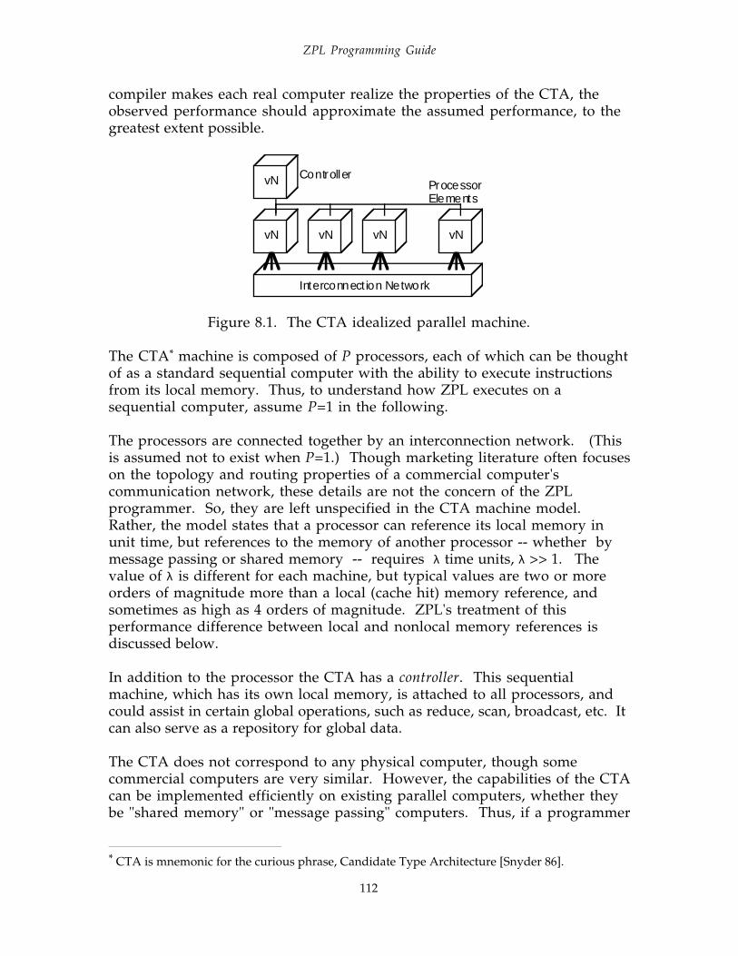
ZPL Programming Guide
112
compiler makes each real computer realize the properties of the CTA, theobserved performance should approximate the assumed performance, to thegreatest extent possible.
vN
Interconnect ion Network
vN vN vN vN
ControllerProcessorElements
Figure 8.1. The CTA idealized parallel machine.
The CTA* machine is composed of P processors, each of which can be thoughtof as a standard sequential computer with the ability to execute instructionsfrom its local memory. Thus, to understand how ZPL executes on asequential computer, assume P=1 in the following.
The processors are connected together by an interconnection network. (Thisis assumed not to exist when P=1.) Though marketing literature often focuseson the topology and routing properties of a commercial computer'scommunication network, these details are not the concern of the ZPLprogrammer. So, they are left unspecified in the CTA machine model.Rather, the model states that a processor can reference its local memory inunit time, but references to the memory of another processor -- whether bymessage passing or shared memory -- requires λ time units, λ >> 1. Thevalue of λ is different for each machine, but typical values are two or moreorders of magnitude more than a local (cache hit) memory reference, andsometimes as high as 4 orders of magnitude. ZPL's treatment of thisperformance difference between local and nonlocal memory references isdiscussed below.
In addition to the processor the CTA has a controller. This sequentialmachine, which has its own local memory, is attached to all processors, andcould assist in certain global operations, such as reduce, scan, broadcast, etc. Itcan also serve as a repository for global data.
The CTA does not correspond to any physical computer, though somecommercial computers are very similar. However, the capabilities of the CTAcan be implemented efficiently on existing parallel computers, whether theybe "shared memory" or "message passing" computers. Thus, if a programmer
* CTA is mnemonic for the curious phrase, Candidate Type Architecture [Snyder 86].

ZPL Programming Guide
113
writes a ZPL program that would be efficient in concept on the CTA, the ZPLcompiler should be able to generate object code for any real machine that isalso efficient [Snyder 94].
For a ZPL program to run on a particular physical computer the compilermust be retargeted to that machine. (This is not a task performed by the ZPLprogrammer.) Retargeting mostly entails interfacing to existing vendor-produced software on the target parallel computer. The base compilertranslates a ZPL program into ANSI C, which, using the retargeted libraries,etc. can be compiled by the native C compiler for the parallel machine. Giventhat the compiler has been retargeted, recompilation of the ZPL compiler'soutput is all that is required for a program to run on a new computer. In thisway ZPL programs are completely portable.
Parallel Execution of ZPL
For the ZPL compiler to produce object code for a parallel computer, it mustallocate data to the computer's memory. The main concern is how to allocatearrays. These are partitioned into sections that are allocated one section toeach processor memory.
Memory Allocation.Scalars in ZPL are replicated across all processors, as are indexed arrays (seenext section).
Parallel arrays in ZPL are partitioned by default into blocks. This partitioningis generally efficient for the operations available in ZPL. The exact blockedpartitioning of the default allocation depends on the dimensionality of thearray:
1-dimensional arrays: The index range including border regions isdivided into P dense subsequences, allocated one per processor.
2-dimensional arrays: The array, including adjacent border regions, isdivided into P dense 2-dimensional subarrays.
k≥3 dimensional arrays: Dimensions 1 -- k-2 are projected to 2-dimensions and allocated as 2 dimensional arrays.
Figure 8.2 illustrates these partitioning rules.
The first thing to notice is that because P is usually smaller than the size ofinteresting arrays, each processor will usually have multiple values stored inits memory, and these values will cover a dense set of indices. Further,values with the same index will be stored on the same processor. This allows

ZPL Programming Guide
114
typical ZPL computations, such as X := Y + Z , to be compiled so a processorcan perform the computation by referencing only local data, i.e. withoutcommunicating with any other processor. For operations such as A@d, thecompiler will usually have to produce data movement commands to transferportions of the array across block boundaries, i. e. move data from processorto processor. However, because the partitioning has the form of dense blocks,most values will not have to move off of the processor. Further, theinterprocessor transfer will move several values at once, which is usuallymore efficient than moving a single value at a time [Choi & Snyder 97].
Figure 8.2. Partitioning of 1D, 2D and 3D arrays for allocation to memories of 4 processors.
Processor Code.In concept the ZPL program can be thought of as executing on the controllerprocessor of the CTA. In this view the scalar variables are stored in thecontroller's memory, and the (parallel) arrays are stored in the memories ofthe other processors. The controller stages the execution of the statements.The processors perform those portions of each statement that apply to datathat is stored on that processor. This view is only conceptual to aid inorganizing the computation.
In actuality ZPL uses a single program, multiple data (SPMD) form ofparallelism, i.e. the compiler generates a single program that is replicated oneach processor.* Expressions involving only scalars or indexed arrays areexecuted by each processor. The compiler creates code for expressionsinvolving regions so that each processor performs that portion of thecomputation applicable to index values of data stored in its memory. When@, wrap , reflect, flood, reduce, scan or permutation operations are required,data transfer instructions are usually performed [Chamberlain et al. 96].
The reduce and scan operations are performed in multiple steps. In the firststep, the operation is performed on local data. Thus, in +<<A the sum of thevalues stored on each processor is computed locally. In the next step these
* SPMD differs from SIMD in that the processors need not execute the same instructionsimultaneously, but rather describe their own path of execution through the common program.
ZPL Programming Guide
115
partial sums are combined. The exact details of this operation differ frommachine to machine: On some machines there is special hardware toperform these operations, e.g. the CM-5. On other machines, this isperformed by a combining "tree" where a group of processors send partialsums to a common processor which produces another partial sum, and passesthis new sum along to another processor to continue the summation. Thistechnique produces the final result in one processor. In the last step ofreduce, the result is broadcast back so that it is known to the other processors.The scan is analogous, though somewhat more complex.
Estimating Program Performance
As with most computer programs it is not possible to know exactly how fast aZPL program will run without executing it on the actual machine, and theperformance will vary from machine to machine. But it is possible to make arough performance estimate based on which operations are expensive andinexpensive. Here, we present the basic performance properties of ZPL.
Full concurrency. Like most languages, the execution time for arrayoperations is proportional to the number of scalar instructions required toimplement the array operation. Thus, the basic computation of the Cannon'salgorithm matrix multiplication program from Figure 6.3
[Res] C := C + A*B;
will require approximately mn multiply instructions, mn add instructionstogether with roughly 3mn loads and mn stores to move the operand valuesfrom the memory back and forth to the processor. There is also a smallamount of overhead required to implement the implied looping.
If the operations are performed on a parallel computer and are roughlyevenly divided among P processors according to the partitioning described inthe last section, then the programmer can expect about P-way speed up. Thatis, the computation will achieve essentially full concurrency. The twoproperties that ensure this desirable result for this statement are
Only element-wise array operations are used, andAll operands refer to elements of the same region.
Statements with these properties should exhibit excellent performance. As afurther assessment for such statements, the performance on a sequentialcomputer is approximately the same as it would be if the equivalent Cprogram had been written.

ZPL Programming Guide
116
Notice that when the arrays are flood arrays the situation can actually beslightly better than described above. Specifically, in the SUMMA algorithmmatrix computation, statement 13 of Figure 6.5
[M] C := C + Af*Bf;
would normally be expected to have the same cost as the analogous Cannon'salgorithm statement from above. But because the flood arrays, Af and Bf , arerepresented by their defining values, the repeated references to these valueswill "hit" in the cache, giving excellent cache behavior.
"@" References.The "@" operator when applied to an operand generally causes some datavalues to be communicated between processors. The key property of thisnearest neighbor communication is that typically only a few values aretransmitted per processor. For example, when the local portion of array Aallocated to processor Pi is a 10 × 10 block, the execution of the statement A :=A@east requires that 10 values be received from the eastern neighbor and 10values be sent to the western neighbor assuming the 2D allocation of Figure8.2. Though the whole array is logically shifted, only a fraction of the valuesare required to change processors and incur communication costs. Theschematic in Figure 8.3 illustrates that only the items along the "edge" of alocal block allocation need to be sent for a "shift by 1." The actual amount ofdata sent for any @ reference depends on the array's size, allocation and thedirection. Moreover, it often happens that a given @ reference will not induceany communication because a previous reference has already caused thecommunication to be performed, and the compiler recognizes that the valuesare still cached [Choi & Snyder 97].
Thus, the nearest neighbor communication generally entails transmittingonly "surface" items of the local allocation, and so performs best on thoseallocations where the surface-to-volume ratio is most favorable. Thoughmore expensive than statements not involving communication, statementsinvolving "@" operators are efficiently implemented and relativelyinexpensive [Chamberlain, Choi & Snyder 97].
Note that from the point of view of estimating execution time, the wrap andreflect operations should also be considered to be nearest neighboroperations.
Strided RegionsIn general, operations over strided regions perform as well as the analogousoperations over non-strided regions, except they are sparser. That is, becausea strided array has fewer elements than a dense array, e.g. a 2D array strided bytwo in each dimension has 1/4 as many elements as the dense array of thesame index ranges, there is proportionately less work performed. Strided

ZPL Programming Guide
117
arrays are allocated "by index," which means that element (i,j) of Astride isstored on the same processor as element (i,j) of Adense . Thus, strided arraysare naturally load-balanced. Strided arrays are stored densely, and so exhibitlocality beneficial to caching.
Pi's block of A Pi+1's valuesneeded by Pi
Pi's values needed by Pi-1
Figure 8.3. Schematic diagram of the values transferred to processor Pi fromPi+1 and from Pi to Pi-1 in evaluating A := A@east .
Reductions/ScansThe algorithms implementing reduce and scan begin by performing theoperation on the block of local data as an intermediate computation. Forexample, the operation +<<A causes each processor to add up the localelements of A allocated to it. The result(s) of the local computations are thenglobally combined. The details of how this is done vary widely depending onthe characteristics of the available hardware. In any case the combining willusually use a technique called the parallel prefix algorithm. This produces asingle, global result that is then broadcast back to each processor. In the case ofreduction the computation is complete, but for a scan the local values must beupdated using the returned intermediate values.
The local portion of the computation will run about as fast as the expression,c+A . The global portion, though difficult to estimate, will generally involvean "accumulation tree," and a "broadcast tree" composed of processors. Thesetrees tend to limit concurrency, since generally only processors at a given"level" in the accumulation tree can be active simultaneously. Thus, reduceand scan are more expensive operations than @ references. Of course, they arealso among the most powerful operations in the language, and generallyworth their cost.
When executed sequentially, reduce and scan are implemented in a direct andefficient manner. As observed in the context of the computation in Chapter4, on parallel machines it can be that reduce and scan are more effective thanrepeated computations involving cheaper operations.
Flooding

ZPL Programming Guide
118
As mentioned frequently, flood arrays are represented using only the definingvalues, i.e. by storing the lower dimensional arrays. So, for example, when arow is replicated by flooding, only the values of that row are stored in theflood array. If necessary, these values will be broadcast to other processors.Though some computers have special assistance for this operation, generallyit should be seen as somewhat more expensive than using "@" operation, butless expensive than performing a reduction or scan.
Scalar computationsScalar quantities are replicated on each processor. Statements involving onlyscalar values, such as
i := i+1;theta := pi/4;
are repeated on each processor. There is no parallelism with this approach,but it is not really feasible to achieve any anyway. Notice that the advantageof replicating the computation compared to computing it on one processorand broadcasting the value is that the replicated computation requires nocommunication.
Indexed arrays are replicated on each processor like scalars. This makesindexed arrays very efficient for representing tables and other constant dataused in computations, because one copy is cached per processor, eliminatingthe need to communicate the values. See the use of the code book, CB, in thevector quantization data compression computation of Chapter 6.
Since ZPL without parallel arrays is mostly a routine sequential language, it isclear that it is perfectly adequate for writing programs for sequentialcomputers. In fact, if the program is not to be run on a parallel computer,then it can be written entirely using indexed arrays and the usual looping.The resulting program's performance will be about the same as a C programfor the sequential machine. There is no parallelism, but this suggests adevelopment approach: write a program using whatever mixture of paralleland indexed arrays that the programmer finds convenient subject to the goalof maximizing the use of parallel arrays. This program will run well onsequential machines. Then, the uses of indexed arrays can be converted toparallel arrays later when a parallel machine is to be used.
PermutationsThe gather and scatter operations (##) are the most expensive operations inZPL, because they can potentially generate two phases of all-to-allcommunication. They are nevertheless useful, and it is often the case thatthere is no efficient alternative to their use. For example, it is possible towrite a transpose without using the permutation operator, but the

ZPL Programming Guide
119
communication required for transposition is inherently expensive onvirtually all computers. So, permutation is as efficient as any solution.
I/OInput and output are expensive in ZPL, just as in all other programminglanguages. One feature of I/O is that it is one of the few places where the ZPLcompiler generates a barrier synchronization.
Summary on Estimation.Though it is not possible to precisely compute a priori the performance of amachine independent program, estimation is possible. For example, the twomatrix multiplication programs given in the last chapter can be comparedbased on the guidelines presented here. Note that for the basic computation,both Cannon's algorithm and the SUMMA algorithm are about the sametime, with some slight advantage to SUMMA for computing with a floodarray. This is partly negated by the slightly greater time to flood as comparedwith shifting the array. So, the two algorithms are essentially the same timeat their cores. However, the Cannon algorithm requires that the two arraysfirst be restructured into a staggered form. This operation is not necessary inthe SUMMA code. So, even though this is only a moderately expensiveoperation, it is clear that the SUMMA algorithm will be more efficient[Chamberlain et al. 98].
Closing Remarks on Performance
Because of basic properties of the ZPL language design, the compiler is capableof producing efficient code. Further, it can perform a variety of optimizationsto reduce both the memory requirements and execution time of the objectprogram. However, nothing contributes to high performance like athoughtfully written program. Thus, the programmer is the most effectiveoptimizer.
The CTA machine model, the brief descriptions of memory allocation,program organization and communication given earlier in this chapterdescribe approximately how the ZPL compiler is likely to organize an objectprogram. It is advisable to keep the following additional points in mindwhen making performance decisions during programming.
• Maximize the use of (parallel) arrays and array-based computation.• Use reduce and scan moderately, since they limit concurrency.• Use permute sparingly.• Express the program directly and succinctly, resisting the temptation to
"program for your implementation."

ZPL Programming Guide
120
The last point cannot be emphasized too much. Most optimizations rely onthe compiler being successful at analyzing a segment of the program.Programs that are convoluted or that use structures designed to "trick" aparticular compiler into producing specific results will almost certainlyfrustrate the analysis of other compilers and greatly limit the program'sportability. If the program is as clean as a classroom example, the compiler islikely to produce textbook example optimizations.
References
B. Chamberlain, S. Choi, E Lewis, C. Lin, L. Snyder and W.Weathersby, 1996"Factor-Join: A Unique Approach to Compiling Array Languages forParallel Machines." Proceedings of Languages andCompilers forParallel Computers, Springer-Verlag.
Bradford L. Chamberlain, Sung-Eun Choi, E Christopher Lewis, Calvin Lin,Lawrence Snyder andW. Derrick Weathersby, "ZPL's WYSIWYGPerformance Model", Proceedings of the IEEE Workshop on High-Level Parallel Programming Models and Supportive Environments(HIPS'98), to appear, March 1998.
B. Chamberlain, S. Choi and L. Snyder, 1997 "IRONMAN: An ArchitectureIndependent Communication Interface for Parallel Computers,"University of Washington TR UW-CSE-97-04-04.
Sung-Eun Choi and Lawrence Snyder, 1997 "Quantifying the Effects ofCommunication Optimizations," International Conference on ParallelProcessing (to appear).
L. Snyder, 1986. "Type Architecture, Shared Memory and the Corollary ofModest Potential," Annal Review of Computer Science, vol. I, AnnualReviews Inc, pp. 289-318.
L. Snyder, 1994. "Foundations of Practical Parallel Programming Languages,"In J. Ferrante and A. J. G. Hey (eds.), Portability and Performance forParallel Processing, John-Wiley & Sons, Ltd., pp. 1-19.

ZPL Programming Guide
121
-- Chapter 9 --
Computational Techniques
As has been observed previously, ZPL is an expressive language thatsimplifies programming because it saves the programmer from specifyingmany low level details like looping and indexing. Perhaps more importantly,by leaving these low level details unspecified, the programmer allows thecompiler the freedom to organize the object code to take advantage of thetarget computer's features. The result is good performance and completemachine independence. So, there is a strong incentive to become fluent inZPL's high level programming style.
In the interest of presenting more examples of high level programming style,this chapter presents a series to "typical programming situations" and theirsolutions in ZPL. The computations considered are
Sequential ComputationInconsequential Code FragmentsSequential routines for promotion
N-Body ComputationsThinking Globally -- Median FindingRandom Number Generation
Programming situations in one area of scientific programming may neverarise in another, so the topics may not apply to all programmers.Nevertheless, they are sufficiently generic, that studying each closely willgenerally provide concepts and knowledge that can be applied often.
Sequential Computation
Achieving parallelism in scientific computations is sufficiently difficult thatthis guide has missed few opportunities to comment on the parallelimplications of a ZPL concept or construct. But, not every program must runon a parallel supercomputer, nor does every part of a supercomputercomputation have to run in parallel. In such situations, ZPL is a finesequential programming language, too.
"Sequential" program text in ZPL is code that will not run in parallel. As ageneral rule computations not involving (parallel) arrays will be sequential.Computations employing only scalars and/or indexed arrays are the primaryinstances of sequential text. For example,

ZPL Programming Guide
122
area := pi * (diam / 2) ^ 2; -- All variables are scalar
and
for i := 1 to m do -- SEQUENTIAL matrix multiply for j := 1 to p do -- using indexed arrays for k := 1 to n do --
C[i,j] := C[i,j] + A[i,k]*B[k,j];
are sequential ZPL text. This is evident since the computations do not use(parallel) arrays.
Sequential and parallel computations, though compiled differently, willperform about the same on a single processor computer. On a parallelcomputer, sequential computations are replicated. That is, each processorperforms the sequential computations redundantly. Thus, sequential andparallel code can be freely intermixed, and when it is executed on parallelcomputers, there will be no overhead for the sequential computations, nor(unfortunately) any speed-up.
Two common cases arise where ZPL programmers find themselves writingsignificant amounts of sequential code: inconsequential code fragments, andsequential routines for promotion. Each will be illustrated.
Inconsequential Code Fragments.There are components of a computation that do not represent a significantfraction of the overall work, but are nevertheless essential to a fullyoperational program. Examples include initialization and problem set up,assessing termination or continuation conditions at the end of loops, errorcorrection or recovery, etc. It is not essential that there be a fully parallelsolution for these components because they contribute so little to the overallrunning time. Indeed, for many of these computations, there probably doesnot exist a parallel solution, and even if there does, it may take more time tolaunch it than can be recovered through speedup. These computations canand should be performed sequentially.
As an example, consider an array A whose m rows must be rearranged beforethe start of the computation, so that their 0th column is in ascending order.This might represent a situation where the 0th column gives key propertiesabout where the data was collected, e.g. latitude.
Since it is assumed that the number m of rows, (but perhaps not their lengthn) is a smallish number, it is decided to perform the sort sequentially. (Thereare parallel sorts, but m is small enough that it is presumed that doing so isnot advantageous.) The solution is to assign the 0th column values into theindexed array Order[1..m] , sort them sequentially, flood the order into aparallel array and then permute the array.

ZPL Programming Guide
123
The indexed array Order is declared
var Order : array [1..m] of pairs;temp : pairs;
where pairs is declared
type pairs = recordval : float;tag : integer;
end;
to have a val field and a tag field. The value will contain the 0th columninformation. The tag is to be initialized to an integer giving the initial orderof the data, and hence the rows. The values and tags are sequentiallyinitialized,
for i := 1 to m do[i,0] Order[i].val := +<< A; -- Val selected from col 0
Order[i].tag := i; -- Tag gives initial order end;
Notice that the contents of the 0th column of the parallel array are extractedand assigned to the sequential array's fields using reduction over a singletonregion. The reduce may seem peculiar, but it is (purposely) the only way toassign a parallel array value to a sequential variable, as a reminder that abroadcast to all processors is required. (See Chapter 8.)
With Order initialized, it is sorted sequentially
for i := 1 to m-1 do -- Sort for j := 2 to m do -- using a if Order[i].val > Order[j].val -- standard
then -- exchangetemp := Order[i]; -- sortOrder[i] := Order[j]; -- which isOrder[j] := temp; -- sequential
end; -- since end; -- Order is anend; -- indexed array
Any sequential sort will suffice.
At this point the val fields are in sequence, and the tag field of item i tellswhich original row of A is to become row i in the reordered A. To implementthis reordering, the tags are stored in a flood array
[1..m,*] Perm := Order[Index1].tag; -- Load order from indexed -- to parallel array

ZPL Programming Guide
124
in preparation for reordering. Notice that the indexed array is subscripted by aparallel array, yielding a parallel result. There is no communication for thisstatement since each processor has a copy of Order . The rows are thenpermuted using the gather form of permutation
[1..m,0..n] A := <## [Perm, ] A; -- Reorder rows
The second reordering array is elided, indicating that the entire row is bemoved as a unit. These last two statements are parallel computations, whichcould be combined
[1..m,0..n] A := <## [Order[Index1].tag, ] A;-- Reorder rows
saving the creation of the Perm variable.
Sequential Routines for PromotionA common way to realize a parallel computation is by performing manyinstances of a basic sequential computation on the elements of a parallelarray. In such cases the base computation will use the sequential componentsof ZPL. These are then applied to the elements of a parallel array bypromotion to achieve the parallel result. This idea has been applied before inthe distance computation for Vector Quantization of Chapter 6. It issufficiently important, however, that it deserves another example.
This illustration will use an optimal global substring match, which is arepresentative computation from the genome sequencing applications area.The task is to locate the best match of a length m candidate sequence Can in alength n primary sequence Prime, m << n. In concept the problem can besolved by considering how well Can matches the first m letters of Prime, i.e.Prime1..m, and giving it a score, and considering how well Can matchesPrime2..m+1, and Prime3..m+2, etc. throughout the whole primary sequence,and then selecting the position with the highest score.
GGCACACTTTCAGTCAAGATATGGTAGACCCACC
CATCan:Prime:
Match against candidate sequence
Obviously, the subroutine for this computation is to figure the score of theCan string against a substring of the Prime string.
The "match" operation is actually a little more complicated than determiningif two letter sequences are identical. Rather, insertions and deletions of lettersare allowed, so two strings are scored by their degree of similarity. Forexample, the candidate string CAT matches the primary string GCAT beginningat the first position by assuming either that there was an insertion of G in the

ZPL Programming Guide
125
primary sequence or the deletion of a G in the candidate sequence. Thecandidate matches exactly when beginning at the second letter of the primarysequence, of course. Since this latter is a more direct match than the former,it is scored higher. Approximate matching, therefore, can be applied to stringsof different length.
The conceptual process behind computing the approximate match betweentwo strings S and T is to imagine filling out a table, in which position i,jgives the score for S[1..i] compared against T[1..j] . An indexed array, V,serves as the table with a row for each S letter and a column for each T letter.(A 0th position handles the case of zero letters, denoted by ∈.) See Figure 9.1
T letter Sequence G C A T C A T 0 -1 -2 -3 -4 0 -1 -2 -3 C -1 -1 1 0 -1 C -1 2 1 0 A -2 -2 0 3 2 A -2 1 4 3 T -3 -3 -1 2 5 T -3 0 3 6
∈∈
S L
ette
rS
eque
nce ∈
∈
Figure 9.1. Matches of CAT against GCAT starting at the first and secondpositions.
After initializing the corner element to zero, a table entry is computed fromthe preceding entries by crediting +2 for a match or -1 for a mismatch. Thus, atable entry i,j is the maximum (best guess) of three quantities:
V[i-1,j]-1 Assumes insertion in S or deletion in TV[i,j] = max if S[i]=T[j] then V[i-1,j-1]+2 else V[i-1,j-1]-1
V[i,j-1]-1 Assumes deletion in S, or insertion in T
Both of the insertion/deletion cases are instances of mismatches. The initialvalues for the 0th row and the 0th column are simply the scores assumingdeletions in S and T (respectively) up to the given position. The result is thelower right corner table entry, i.e. V[m,n] .
A key observation is that the whole table does not have to be kept, since byfilling it out column-wise, only the previous column or the previous entry inthe same column is ever referenced. Hence, only one column needs to berepresented, motivating the sequential procedure shown in Figure 9.2 tocompute the score.
This sequential procedure score takes the S string and one letter of the Tstring as "by-reference" (var ) parameters, meaning they will be referencedexternally and not actually "passed in". Additionally, the position, pos , of theletter t from the start of string T is passed in for use in initializing the 0th
entry in the column. The column V is also referenced externally. The logic of

ZPL Programming Guide
126
the routine is simply to work down the column, using the previous entries tocreate new ones.
To put the whole computation together, the sequential procedure score willbe applied at each position of the primary string, producing a parallelcomputation. First, data structures for the candidate and primary strings aredeclared
1 procedure score( 2 var S : array[0..m] of ubyte,-- Indexed array of string 3 pos : shortint, -- Position of T considered 4 var t : ubyte, -- Letter in T[pos] 5 var V : array [0..m] of shortint --Index array of col below 6 -- T[pos-1] updated to T[pos] 7 ): shortint; -- Return the best score 8 var i, -- Index 9 best, -- Highest score in column10 mtch, -- Temp to compute match11 last: shortint; -- Temp to save previous entry12 begin13 last := V[0]; -- from overwrite14 V[0] := - pos; -- Initialize first entry15 best := - pos; -- Initialize maximum score16 for i := 1 to m do -- Working down the column17 if S[i] = t then mtch := 2 else mtch := -1 end;18 mtch := mtch + last; -- Result of compare + diag19 last := V[i]; -- Grab next before overwrite20 V[i]:=max3(mtch,V[i-1]-1,V[i]-1);-- Compute scores, pick max21 if V[i] > best then best := V[i] end;-- Save best score22 end;23 return best; -- Report back24 end;
1 procedure max3(x, y, z : shortint) : shortint; 2 begin 3 if x >= y & x >= z then return x; end; 4 if y >= x & y >= z then return y; end; 5 if z >= x & z >= y then return z; end; 6 end;
Figure 9.2. The score procedure and the auxiliary max3 procedure.
var Can : [0..m] array of ubyte; -- Indexed array for Candidate Prime : [1..n] ubyte; -- Parallel array for Primary Vee : [1..n] array [0..m] of shortint; -- Parallel array of
-- indexed arrays representing-- a column of each table
Best : [1..n] shortint; -- Parallel array of scores
as well as the parallel array Vee of columns. The ith element of Vee willrepresent the current (pos ) column of the table for the match starting at the

ZPL Programming Guide
127
ith position of Prime , its maximum score to this point will be in the ith
element of Best . After declaring a
direction right = [1];
and initializing Best and all of the columns of Vee to their proper 0th
column values,
Best := 0;for i := 0 to m do Vee[i] := -i; end;
the data can be read in. Once Can and Prime contain their proper letterstrings, the loop
for j := 1 to m do[1..n-j+1] Best := max(Best, score(Can, j, Prime, Vee)); [1..n-j] Prime := Prime@right; end;
produces the desired result. (The iteration would likely continue beyond mcycles to provide for insertions in T.)
The score procedure is called with parallel arrays Prime and Veecorresponding to scalar t and indexed array V, respectively, in the procedureheader. This creates a parallel computation in which the sequentialprocedure is promoted to apply to each position. The use of "by-reference"parameters assures that there will be but one copy of the basic data structures.The shift of Prime brings the next letter position into consideration. Noticethat the regions limit the computation to those positions of Prime for whichthe Can string does not "fall off of the end".
The relevant entries for Vee assuming Can ≡ CAT and Prime ≡ GCAT are
0 0 0 0 -1 -1 -1 -1 -2 -2 -2 x -3 -3 x x-1 -1 -1 -1 -1 2 -1 -1 1 1 -2 x 0 0 x x-2 -2 -2 -2 -2 1 -2 -2 0 4 -3 x 3 3 x x-3 -3 -3 -3 -3 0 -3 -3 -1 3 -4 x 2 6 x x Initial j=1 j=2 j=3
Notice that columns 1 and 2 in each snapshot correspond to the ith columnsin the tables shown in Figure 9.1.
Of course, the best score is found by
... max<< Best ...
and the positions of the best matches are given by the nonzero items in theexpression

ZPL Programming Guide
128
... Index1*(Best = max<<Best) ...
which could be printed out or participate in other computations.
In summary, ZPL keeps a reasonably strict separation between the paralleland sequential features of the language so that programmers can always beaware of how their code will be executed. However, by promoting sequentialcomputations to apply to the elements of parallel arrays, efficient parallelcomputations are created.
N-Body Computations
Many problems involve the motion of bodies in space. If space can beuniformly decomposed, the most straight forward ZPL representation is anarray whose elements are lists of the bodies. The array represents thedecomposition of space, and the body lists are maintained in user-managedindexed arrays. Each cell in the decomposition is processed in parallel,making this an instance of the promoted sequential routines discussed in thelast section. This N-body solution is most effective when certain propertiesare present:• If every cell of the decomposition contains a reasonable number of bodies
and the ratio between the number of bodies in the sparsest to densest cellis not too extreme, e.g. 1:3, say, rather than 1:10,000, then the work will bebalanced.
• If there is a reliable (though perhaps not perfect) upper limit on thenumber of bodies in a block, then the storage allocated for the lists can bemanaged more easily.
Many, but not all N-body problems fulfill these conditions. Even when theydo not, ZPL can be used for a solution, though the performance might fallbelow expectations.
To illustrate sample N-body computations, postulate that 2D space has beendecomposed into an n × n mesh of cells, and that the maximum number ofbodies in any cell is m. (The generalization to 3D is obvious.)
constant m: integer = 100; -- max particles per celln: integer = 16; -- # of cells on side of mesh
These parameters are assigned typical values, which will probably be revisedwhen tuning the program for performance. The region of the computation is
region R = [1..n, 1..n]; -- Problem mesh, representing -- partitioned 2D space
The array containing the m-element lists of bodies

ZPL Programming Guide
129
var Parts: [R] array [1..m] of particle;
is declared, where a particle is represented by a record
type particle = record -- Particles are triples of x, -- Position x coord y, -- Position y coord v: float end; -- and value
containing three values. True N-body computations would use morecomplete representations for the bodies, of course, but these suffice here.
Each cell will, generally, not have exactly 100 particles in it, so it is necessary tokeep a count of the number of particles actually present. This count is also a(parallel) array because there is a different count for each cell. Continuing thevariable declarations,
C: [R] shortint; -- Particles per cell <= 16K
provides a short integer for the count for each cell, as illustrated in Figure 9.3.
Parts
6 3 6 24 2 6 67 5 8 43 6 5 5
CFigure 9.3. Illustration of Body and C arrays for n=4, m=8.
An important programming convention will be that the particles will be keptat the "front" of the lists, with the unused particle positions at the higherindices. Thus, elements of Parts that are occupied have index positions1..C .
The coordinates of each cell in space will be represented by the positions of itslower left and upper right corners. These could be represented by recordswith a pair of values for each corner's x,y coordinates, but since thecoordinates are never used as a unit, bundling them together is unnecessary.Arrays of scalar values are, therefore, preferred.
LoX, LoY, HiX, HiY: [R] float;
Though shortint might seem to be a better choice than float when space hasbeen decomposed into integral sizes, it is more efficient to use float arrays toreduce type conversions in comparisons with elements of Parts .

ZPL Programming Guide
130
To complete the declarations, array temporaries and a scalar index aredefined.
Temp: [R] particle;T, P: [R] shortint; i: shortint;
Temp is an array that stores one particle per index position, T is another arraystoring an index of a particle list position, P is a flag array indicating (1 or 0)whether or not a moving particle has been found, and i is a scalar loop index.
Single Particle PushingTo illustrate basic N-body manipulations, consider implementing the motionof single particles moving out of cells in a single direction, say north . Thissolution can be generalized to move more particles in multiple directions.The approach is to iterate (for all cells in parallel) through the particle listslooking for a particle whose updated position is outside the cell to the north .Those that are found, are removed from the lists, the lists are compacted tokeep them dense, and the counts of particles are corrected. The particles arethen sent to their neighbors and incorporated into the particle lists at thedestinations. The computation has the following components:
• Initialization• Find a departing particle• Compact the list• Move the particle• Incorporate it into its new cell
These components will now be described. The overall one-direction, one-particle code is shown in Figure 9.4.
Initialization. It is assumed the computation is underway, and that thepositions of all particles have been updated. Those whose new position isbeyond the limits of their cell are to be moved. The initialization is
T := C + 1; -- Start position of mover 1 past endP := 0; -- Flag for found particle set at none
which indicate that no departing particle has yet been found.
Find departing particles. Shattered control flow, indicated by the use of thearray C in the for -loop statement, is used to sweep through the particle listsof the cells looking for a north moving particle.
/* Find Departed Particle */for i := 1 to C do -- Loop thru particles of each cell if Parts[i].y > HiY -- Particle headed north?
then -- Yes P := 1; -- Record that one has been found Temp := Parts[i]; -- Grab the particle

ZPL Programming Guide
131
T := i; -- Record where it is located exit; -- Interrupt loop as particle found
end;end;
Recall that since this is a shattered for -loop, there are n2 (parallel) iterations,one for each cell, ranging over the intervals 1 to C, i.e. the loop for cell u,vranges from 1 to Cu,v. The y coordinate of the i th particle in the list iscompared with the HiY coordinate of the upper right corner of the cell. Theloop is exited for each cell when a departing particle is discovered.
Compact the lists. It is presumed that some particles are departing, i.e. T !=C+1, though it is not necessary. The vacated space is compacted, usinganother shattered for -loop.
/* If Vacated, Compact list */for i := T+1 to C do -- Loop from point of interruption Parts[i-1] := Parts[i]; -- Scooch 'em upend;C := C - P; -- Reduce count if particle left
Having initialized T to be one position beyond the end of the list, i.e. C+1, thecompaction loop falls through in the case no north moving particle wasdiscovered in a give cell.
Move the particles. To move particles to the north requires that both theirmotion and the effects along the borders be considered. An assignment suchas
Temp@north := Temp; -- Send particle north
would seem to be the obvious statement, but it has the effect of modifying thenorth border of Temp plus all elements of the Temp array except the bottomrow, i.e. it doesn't incorporate particles from the south border. Assumingthat particles are to be lost when they move off the top edge, and that particlesare to be introduced along the south edge
[R at south] Temp@north := Temp; -- Send particles north
would have the proper affect provided the southern border of Temp had beenset up to introduce particles. The right-hand side of the statement wouldrefer to the southerly cells from which particles come, while the left-handside would simply refer to Temp, i.e. the @north and at south cancel. Anentirely equivalent construction, and probably somewhat more transparent, is
Temp:= Temp@south; -- Get particles moving north
ZPL Programming Guide
132
which focuses on where the particles are coming from rather than where theyare going to. This is the desired construction, and we apply it a second time torecord the arrival of a particle
P := P@south; -- Indicate arriving particle
Notice that even when no particles are moving, the Temp array will transmitvalues. These are meaningless, which is why transmitting P, the indicator ofuseful data, is also required. It is possible to set up the computation to moveactual particles only, but this is probably more expensive than treating themuniformly.
Incorporate new point. After the particles have been moved to the neighbor,the processing continues to include the newly arrived particle in the list.
/* Incorporate particle */C := C + P; -- If particle arrived, bump countParts[C+1-P] := Temp; -- Add to list, or no-op if none
P is 1 if a valid particle was sent, and 0 otherwise, so adding it to C changes thecount only for those cells where points just arrived. By indexing Parts asshown, Temp is incorporated as the new last item (valid data sent and P=1), orunknown values are stored in the first free position of the particle list(invalid data sent and P=0).
The one-particle-per-cell solution is complete. It will sweep through theentire particle list for each cell removed. This is perhaps too much "work"for the result achieved. Removing more items at a time will reduce theoverall computational work, and lead to a more efficient program.
Batched Pushing SolutionGeneralizing the one-particle-per-cell solution is straightforward. Thenumber of particles to be treated in a batch will be a parameter to thecomputation, so that the program can be conveniently customized to beoptimal for the target computer. The declaration
constant b: integer = 5; -- # of particles in batch
is to be added to the variable declarations section given above.
Next, the Temp variable, which is used to hold and transmit the particles,must be redeclared to have space enough to store the whole batch. Theprevious declaration for Temp is revised as follows
Temp: [R] array [1..b] of particle;

ZPL Programming Guide
133
upgrading Temp to a (parallel) array of b-element linear arrays, each elementbeing a particle .
Finally, by reinterpreting the flag array P from signaling that a movingparticle has been found to counting the number of moving particles found,the previous code is easily rewritten. See Figure 9.5. Indeed, notice that theone-particle-per-cell program can be interpreted as the batch size of 1 case, i.e.b=1 .
1 [R] begin /* Initialize */ 2 T := C + 1; -- Start position of mover 1 past end 3 P := 0; -- Flag for found particle set at none 4 5 /* Find Departed Particle */ 6 for i := 1 to C do -- Loop thru particles of each cell 7 if Parts[i].y > HiY -- Particle headed N? 8 then -- Yes 9 P := 1; -- Record that one has been found10 Temp := Parts[i];-- Grab the particle11 T := i; -- Record where it is located12 exit; -- Interrupt loop as particle found13 end;14 end;1516 /* If Vacated, Compact list */17 for i := T+1 to C do -- Loop from point of interruption18 Parts[i-1] := Parts[i];--Scooch 'em up19 end;20 C := C - P; -- Reduce count if particle left2122 /* Move Particle */23 Temp := Temp@south; -- Send particle N24 P := P@south; -- Send indicator of arrived point2526 /* Incorporate particle */27 C := C + P; -- If particle arrived, bump count28 Parts[C+1-P] := Temp; -- Add to list, or no-op if none29 end;
Figure 9.4. One-particle-per-cell solution for
There are two noticeable changes to the program. First, as the particle list isscanned looking for moving particles, the loop is not interrupted until a fullbatch is formed. So, part of the compaction operation is incorporated into thesearch loop. The loop is exited when the batch has filled. The other changeis in the code incorporating arrived particles into the list. The previousassignment became a loop, and it was more convenient to update the countvariable after the items had been added. Notice that if no variables are sent,control falls through the loop and updating the count is a no-op.
The application of this program is as follows. The batch size b is set to, say,the expected number of north moving points, determined through some

ZPL Programming Guide
134
experimentation. Then, batches are moved in a loop which continues as longas north moving particles remain in any cell, i.e. 0 != +<<P . The concept isthat for problems meeting the properties mentioned at the beginning, a smallnumber of iterations (2-3) should suffice to move the particles. This doubtlessleads to a more efficient solution that doing the transfer all at once, whichwould require a worst-case batch size, and is far more expedient than writingZPL code to work out the actual number of items moving and thentransferring the exact number. The principle is that in parallel computing itis often more effective to perform some redundant computation to reduce thecritical path.
1 [R] begin /* Initialize */ 2 T := C + 1; -- Start interrupt position at end+1 3 P := 0; -- Number found starts at 0 4 5 /* Find Departed Particles */ 6 for i := 1 to C do -- Loop thru particles of each cell 7 if Parts[i].y > HiY -- Particle headed N? 8 then -- Yes 9 P := P + 1; -- Record that one has been found10 Temp[P] := Parts[i]; -- Grab particle11 T := i; -- Record where it is located12 if P=b then exit; end;-- Interrupt loop since batch filled13 else14 Parts[i-P] := Parts[i]; --Scooch up particles15 end;16 end;1718 /* Complete Compacting list */19 for i := T+1 to C do -- Loop from point of interruption20 Parts[i-P] := Parts[i]; --Scooch 'em up21 end;22 C := C - P; -- Reduce count by number leaving2324 /* Move Particles */25 Temp := Temp@south; -- Send particles N26 P := P@south; -- Send count of arrived particles2728 /* Incorporate particles */29 for i := 1 to P do30 Parts[C+i] := Temp[i]; -- Add to list, or no-op if none31 end;32 C := C + P; -- If particle arrived, bump count33 end;
Figure 9.5. Batched particle solution for pushing points north.
Thinking Globally -- Median Finding
Finding the median of a set of numbers is a simple computation when the sethas been sorted -- select the middle item. But, if the set does not need to besorted for other reasons, then the median can be found directly. The

ZPL Programming Guide
135
following program finds the median directly by keeping an interval lo:hithat bounds the median, estimating the median by the midpoint of theinterval, computing which half contains the median and then collapsing theinterval by "discarding" the other half. Convergence is achieved when theendpoints meet. Though this is a simple computation, it provides anopportunity to illustrate thinking globally.
The solution requires a linear region,
region R = [1..n];
the array containing the data and an array for masking,
var A : [R] float; M : [R] ubyte;
and some scalar variables to support the computation,
var lo, hi,
mid: float; count: integer;
Notice that the values are chosen to be of floating-point type, but other typescan be handled simply by changing declarations.
The strategy is to begin with an interval that spans the whole set of numbers,
lo := min<< A;hi := max<< A;
and then to shrink it iteratively
[R] while hi != lo do mid := (hi - lo)/2; -- Figure midpoint M := A < (lo + mid); -- Which items are smaller count := +<< M; -- How many are there if count < ceil(n/2) -- Is median in upper half? then [" without M] lo := min<< A; -- Yes, move lo up else [" with M] hi := max<< A; -- No, move hi down end; end;
The computation proceeds as follows. If the values between lo and hiinclusive are the same, then that value is the median value. Otherwise, themid point between the two endpoints is determined, and a mask, M, iscomputed with a 1 set for each element less than the mid point. The totalcount of these elements is then computed. If count is less than n/2, then the

ZPL Programming Guide
136
median element must be in the half larger than mid, and lo should beadjusted up. Otherwise, hi should be adjusted down.
The adjustment masks the R region to consider the indices of only a subset ofthe elements. (Recall that ditto (" ) is synonymous with "the current region.")When the mask employs the without operator, the elements larger than orequal to the mid point (corresponding to zeroes of M) are considered, and theminimum of these elements becomes the new lo endpoint. Symmetrically,when the mask employs the with operator, the elements smaller than themid point (corresponding to ones) are considered, and the maximum of thesebecomes the new hi endpoint. The iteration continues until the intervalcollapses.
It is instructive to consider the convergence of the algorithm. Consider firstthe case when A has Index1 as its value. The snapshot of the relevantprogram variables (prior to the if -statement) of each iteration is shown.(The values do not have to be in order to produce this result, of course, butorder makes the logic somewhat easier to follow.)
Array A lo hi mid Array M count1 2 3 4 5 6 7 8 9 1 9 4 1 1 1 1 0 0 0 0 0 4
5 9 2 1 1 1 1 1 1 0 0 0 6 5 6 0.5 1 1 1 1 1 0 0 0 0 5 5 5
The three iteration convergence illustrated is not dependent on the value ofn. A moment's thought indicates that any odd length sequence ofconsecutive integers converges in three steps, because the first iteration willthrow out all elements below the median, the second will purge those abovethe median+1, and the last will shrink this two element interval to a singleelement. (An array of identical values doesn't iterate.) In general, thealgorithm uses a Fibonacci search to push the end points toward the median.
Readers who are conversant with ZPL's WYSIWYG performance model willnotice the repeated use of reduction operations. Though efficientlyimplemented, reduction is a global operation requiring communication andit is generally a good principle to reduce its use when possible. In the medianprogram, as with many computations, reduction is essential.
Random Number Generation
Computers do not generate truly random numbers, of course, thoughsometimes a buggy program will seem to the frustrated programmer to bedoing so. Rather, they generate pseudo-random numbers -- a finite sequenceof dependent numbers that over the sequence appears to have the statisticalproperties of random quantities. The generation of pseudo-random numbers

ZPL Programming Guide
137
is a deep and interesting topic in computer science, and the reader is warnedthat generating pseudo-random numbers by "random" methods doesn't work[Knuth 69]. Consequently, since random numbers are widely used inscientific computations, they are briefly considered here.
A reliable technique for generating high quality pseudo-random numbers oncontemporary machines having 32-bit integer arithmetic is the Learmonth-Lewis prime-modulus multiplicative congruential generator [Learmonth &Lewis 74],
rn = 16807rn-1 mod (231-1)
where r0, called the seed, is given initially. The sequence sweeps through thefull range of positive integers for 32-bit twos complement representation, {1,..., 231-2}, two billion numbers in all, before repeating. (Zero could not begenerated, of course, since to do so would kill the sequence.)
The Learmonth-Lewis generator can be converted into a scalar ZPL functiondirectly. It is convenient to define a constant for the modulus, so that it neednot be continually recomputed,
constant llmodulus : uinteger = 2147483647;-- Set modulus to 2^31 - 1
multiplier: uinteger = 16807; -- Set multiplier to 7^5recipmod : double = 4.6566128752457969E-10;
-- Reciprocal of modulus
as well as the multiplier and the reciprocal of the modulus. Also, declare
var seed : uinteger;
and initialize it
seed = 377003613; -- Set seed
with some arbitrary value. This value can be changed for production runs,say with the time of day. Specifying a fixed initial value assures thatdebugging runs are repeatable.
The scalar function
procedure llrand(var rsequence: uinteger) : uinteger;/* Learmonth-Lewis random number generator for 32-bit arithmetic */var rhi, rmlo, fhi : uinteger;begin
rhi := bsr(rsequence, 16);rmlo:= (bsr(bsl(rsequence, 16), 16) * multiplier;fhi := rhi * multiplier + bsr(rmlo, 16);rsequence := (bsr(bsl(rmlo, 16), 16) + bsr(bsl(fhi, 17), 1))

ZPL Programming Guide
138
+ bsr(fhi, 15);if rsequence >= llmodulus then rsequence -= llmodulus;end;return rsequence;
end;
takes rn-1 in as a var parameter, i.e. rsequence is by-reference, and producesrn. The involved right and left shifting is designed to assure that the large,intermediate products do not cause overflow.
This function is invoked with the call
... llrand(seed) ...
whenever a random (scalar) integer value is needed. If random floating pointnumbers are desired, then changing the procedure's return type to doubleand changing the next to last line to
return rsequence * recipmod;
produces uniformly distributed random floating point numbers over (0,1).
The llrand procedure can be tested by beginning with the previouslyinitialized seed and comparing with the following test sequence, which haselements separated by 100,000 llrand calls:
r0 = 377,003,613r100,000 = 648,473,574r200,000 = 1,396,717,869r300,000 = 2,027,350,275r400,000 = 1,356,162,430
An important point to notice is that because seed is a scalar, ZPL willreplicate its value on every processor, as explained in Chapter 8. Accordingly,when llrand is called, every processor will produce the same pseudo-random scalar value. This can be used like all other scalars in ZPL.
For cases where an array, A, is to be initialized to random values, the code
/* Set A to a random initial value */ for i := 1 to n do
for j := 1 to m do[i,j] A := llrand(seed); (*) end;
end;

ZPL Programming Guide
139
performs the operations such that the sequence r1, r2, ... is assigned toelements of A in row-major order.
The loops initialize the array one position at a time, and since this is asequence, the computation is sequential. That is, by using a single pointregion within the loops, all rmn elements are swept through one at a time.Notice that each processor will execute this loop ensuring that all processorshave the same seed value upon completion. The process is fast, and is likelyto contribute negligibly to the overall execution time of any seriouscomputation, so alternative initializations are not considered.
A final cautionary note about arrays of random numbers. The llrandprocedure given above is scalar, and could be promoted to compute over anarray, just like any scalar procedure. Array sequences of random numberscould be generated by promoting llrand to apply to an array Seed, providedit is initialized properly. The initialization (*) above is not appropriate forthis application. This is because the kth element in the sequence of Seed ij+1 isthe k+1st element of the sequence for Seed ij. That is, the elements arecorrelated. Thus, the previous initialization is ideal for single uses such asinitialization, but not for array sequences of random numbers.
References
Donald E. Knuth, 1969 The Art of Computer Programming, Vol. 2,Seminumerical Algorithms, Addison-Wesley.
G. P. Learmonth and P. A. W. Lewis, 1974 "Statistical tests of some widelyused and recently proposed uniform random number generators,"Proceedings of the 7th Conference on Computer Science and StatisticalInterface.

ZPL Programming Guide
140
-- Chapter 10 --
ZPL and Future Parallel Programming
ZPL has introduced a series of new, high level programming concepts tosimplify the task of parallel computing, and in addition, simplified knowntechniques such as array manipulation. Perhaps the most significantcontribution is the WYSIWYG performance estimation capability.Throughout the language, regions are key to making clean, easy-to-useprogramming facilities. What more could be done? Plenty.
On the horizon is Advanced ZPL, a superset of ZPL -- all ZPL programs arelegal A-ZPL programs -- in which there are more sophisticated datastructuring facilities, more powerful programming facilities, e.g. pipelining,and more tightly integrated tools. Advanced ZPL will elevate programmingto a higher level of abstraction subject to the conditions that ZPL's highperformance and portability be maintained.

ZPL Programming Guide
141
ZPL REFERENCEExamples of the most common features of ZPL
BASE TYPES: REGION OPERATORS: CONTROL: {}=optional, {{}}=0/moreSigned Unsigned at translate [R at east] if ... then ...{else ...}end;
file of border exterior [east of R] if ... then ... {{elsif ... }}string in border interior [east in R] {else ...} end;boolean by stride [0..n-1 by 2] for i:=1 to n {by 2}char with mask [R with M] do ... end;
sbyte ubyte without antimask [R without M] while ... do ... end;shortint ushortint empty inherit dim [ , 2 .. n-1] repeat ... until ... ;integer uinteger " inherit region [" at east] begin ... end;longint ulongint return ... ; from procedurefloat • of and in compose inside-out • exit; from innermost loopdouble • at composes by adding directions • continue; to next loop iter.quad halt; terminate execution
OPERATORSArithmetic Relational Logical Bitwise Assignment Precedence+ addition = equality ! not bnot(a) complement := + - ! High- subtraction != inequality & and band(a,b) and += << || >> ##* multiplication < less than | or bor(a,b) or -= ^/ division > greater than bxor(a,b) exclusive or *= * / %^ exponentiation <= less than bsl(s,amt) left shift /= + - (binary)+ unary plus or equal to bsr(s,amt) right shift %= = != < > <= >=- negation >= greater than &= & | Low% modulus or equal to • Left Associative • |=
ARRAY OPERATORS (A = 2D array over [1..n,1..n] )+<<A Full reduce >##[n-Index1+1,]A Scatter Permute[1..n,1] ...*<<[R] A Partial reduce [east of R] wrap A; Periodic border+|| A Full scan [east of R] reflect A; Mirror Border*||[2] A Partial scan if A<0 then ... end; Shattered i f[R] ... >>[1..n,1] A Flood for I:= 1 to A do ... end; Shattered for<##[Index2,Index1]A Gather Permute while A>0 do ... end; Shattered while
SAMPLE DECLARATIONSprogram Sample; Program header lineconfig var n : integer = 100; Define, set; command line changeableconstant yr : float = 365.25; Define, set; fixedtype triple = array[1..3] of ubyte; Defined type; indexed array of bytesvar U, V : triple; Declare vars; reference as U[2]type posish = record Define type of three values lat, long : float; Field name(s) and type height: integer; end; Field list ends with endvar Summit:array[1..50] of posish; Declare vars; ref as Summit[2].latregion R = [1..n, 1..n]; Named region
St = [1..n, 1..n by [2,2]]; Region strided by 2 in each dimensiondirection east = [0, 1]; Define directionvar A, B, C : [R] double; Declare arraysprototype abs(x:float) : float; Procedure prototypeprocedure abs(x:float) : float; Procedure declaration begin if x<0 then return -x else return x; end;
© 1998 University of Washington

ZPL Programming Guide
142
Fundamental Constants, Standard Functionsand Timers
ZPL provides access to a set of built-in facilities to simplify programming.The fundamental constants and standard scientific functions come from the Clanguage's math.h library on the host computer.
Fundamental Constants. The following double precision floating pointconstants are provided:
Name Meaning Decimal Valuem_e e 2.7182818284590452354m_log2e log2 e 1.4426950408889634074m_log10e log10 e 0.43429448190325182765m_ln2 loge 2 0.69314718055994530942m_ln10 loge 10 2.30258509299404568402m_pi π 3.14159265358979323846m_pi_2 π/2 1.57079632679489661923m_pi_4 π/4 0.78539816339744830962m_1_pi 1/ π 0.31830988618379067154m_2_pi 2/ π 0.63661977236758134308m_2_sqrtpi 2/ √π 1.12837916709551257390m_sqrt2 √2 1.41421356237309504880m_sqrt_2 1/ √2 0.70710678118654752440
Scientific Functions
The following standard scientific functions are provided in multiple forms,one generic form and other type-specific forms. Use of the generic functionwill result in the compiler generating a call to the proper type-specific libraryroutine matching the argument type or higher argument type when there aretwo arguments.
Name Meaningabs(x) Absolute value of xacos(x) Arc cosine of xasine(x) Arc sine of xatan(x) Arc tangent of xatan2(x,y) Arc tan of x/yceil(x) Least integer not less than x

ZPL Programming Guide
143
cos(x) Cosinecosh(x) Hyperbolic cosinecube(x) x3
exp(x) ex
floor(x) Greatest integer not greater than xfmod(x,y) Floating point remainder of x/yldexp(x,y) x2y
log(x) Logarithm to base e of xlog2(x) Logarithm to base 2 of xlog10(x) Logarithm to base 10 of xpow(x,y) xy
sin(x) Sine of xsinh(x) Hyperbolic sine of xsqrt(x) Squareroot of xtan(x) Tangent of xtanh(x) Hyperbolic tangent of xtrunc(x) Truncate x to a whole number
Type-specific standard functions can be called explicitly. To construct thename of a type-specific standard function, append the type designationletter(s) to the generic function name, precision first. The type designationletters are
f = single precision floating point,d = double precision floating point,q = quad precision floating point,c = complex
For example, sin(x) calls the sine function matching the type of x ; sinf(x)is the single precision sine function, sind(x) is the double precision sine,sinq(x) is the quad precision sine when quad precision is available, andsinfc(x) , sindc(x) and sinqc(x) are the corresponding complex calls.Arguments not matching the type of type-specific standard function areconverted.
Timers
Two timing functions are provided based on the native timer of the hostcomputer. Timing granularity varies widely, and is not always very fine.Accordingly, timing very small sections of program can be inaccurate.
ResetTimer() Resets the timer to zero and returns a double precisionfloating point number that is the number of seconds sincethe last call to ResetTimer() .

ZPL Programming Guide
144
CheckTimer() Returns a double precision floating point numberthat is the number of seconds since the last call toResetTimer() .
Check your installation's documentation for details.

ZPL Programming Guide
145
Index0-origin 201-origin 34actual parameter 73, 75add 13Advanced ZPL 140aggregate 100, 105and 13and-equals 16applicable region 32, 40approximate match 125arguments 71, 72arithmetic operators 13, 14array 12, 21, 22, 40, 63, 105, 119, 121, 122, 124array coordinates 29array keyword 61assignment 16, 31, 33assignment symbol 4, 16associativity 14, 35at 56base direction 102, 103base region 25, 26, 98, 99base types 14, 64begin 16, 17binary files 41binary I/O 41binary operators 14bitwise and 13bitwise exclusive or 13bitwise not 13bitwise operators 13bitwise or 13boolean 12, 14border region 100, 113borders 6, 26, 27, 131boundary conditions 6, 26, 28brace pair 102, 103brackets 20, 21, 22, 35, 72, 90bread() 41bwrite() 41by 16, 17, 98by-reference 71, 73, 75, 125, 127, 138by-value 73Cannon's algorithm 82, 115, 116, 119
ZPL Programming Guide
146
capitals-for-arrays policy 16Cartesian coordinates 29Cartesian product 19, 21case sensitive 15char 12, 14character 12, 14check-pointing 41close() 41, 44colon 21command line 37comment terminator 4commenting 18communication 116compiler 113complement 13composition 56, 57compound statement 17, 78compression 93, 118config var 37configuration parameter 8connected component 51constant 37continue 16, 17control-flow 16, 17, 75, 81conversion of numbers 15correlation coefficient 43coversion of lower type 15CTA 111, 112, 114, 119d-dimensional array 12data types 12declaration 83degenerate range 55dense array 116dense indices 99derived types 12deterministic 109dimension 20, 98, 108, 113dimension specifiers 35direction 5, 13, 24, 25, 27, 37, 56, 83, 89, 98, 99, 101, 102, 103, 104ditto 60, 61, 73, 136divide 13, 14divide-equals 16do 16, 17dot notation 64double 12, 14double brackets 60

ZPL Programming Guide
147
double dots 20double precision 12, 14dynamic region 58, 59, 103dynamic strided region 99elementwise 7, 30else 16, 17, 18elsif 16, 17, 18empty braces 105end 16, 17, 18end-of-line 4equal 13, 14equal precedence 14equal sign 4exit 16, 17exponent 14exponentiate 13, 14false 14file 12, 39, 41file declaration 39file descriptor 40, 41, 43first dimension 21first quadrant 30float 12, 14floating point 12floating point arithmetic 35flood 10, 69, 109, 114, 122flood array 66, 110, 116, 118, 119flood region 65floodable dimension 65flooding 91for 16, 17for-loop 47formal parameter 71, 73full concurrency 115fundamental constants 142gather 107, 108, 118goto 17greater than 13, 14greater than or equal 13, 14halt 16, 17hierarchy 104, 105histogram 45, 91idealized parallel computer 111identifier 15identity matrix 33if 16, 17, 18

ZPL Programming Guide
148
if-statement 47implicitly parallel 1, 111in 57indenting 18index range 25index set 21, 27index tuples 20indexd 31, 32, 33, 110indexed array 12, 61, 73, 93, 95, 114, 118, 121, 124inheritance 60, 66input/output 39integer 12, 14iteration variable 17Jacobi program 2, 4keywords 16leading blanks 18less than 13, 14less than or equal 13, 14letters 15Levialdi 51load-balance 117locality 9logical and 13, 14logical array 91logical data 12, 14logical false 14, 45logical operators 13, 14logical or 13, 14logical true 14, 45logical vectors 42, 46, 47longint 12, 14lossy compression 93lower and upper limits 19lower limit 20machine independence 121machine independent 1, 111machine specific libraries 15main_program 37mask 77, 95, 136matrix multiplication 10, 81, 86, 87, 88, 115median 134memory 113, 115, 119minus-equals 16mirrored 28mod-equals 16modulo 13, 14

ZPL Programming Guide
149
mu 42, 43multiarray 105multidirection 102, 103, 104multigrid 98multiple region specifiers 23multiply 13, 14multiregion 104, 105N-body 128, 129named regions 22negate 13, 14negative offset 24, 29not 13, 14not first class 13, 21numerals 15numeric types 15object code 15of 57offset 24offset-referencing 26offsets 24op-scan 35open() 40, 41, 43optimizations 120or 13or-equals 16order of accumulation 35parallel array 13parallel computer 118parallel execution 111parallel prefix 69, 91, 117parameter 73parentheses 14, 43partial reduce 35, 67, 69, 70, 91, 92partial scan 35, 69performance 2, 9performance estimate 115periodic 28permutation 107, 108, 109, 114, 118, 124permutation specifier 108plus-equals 16plus-scan 35, 50, 91portability 120, 140positive offset 24, 29pow 14precedence 14precision 12

ZPL Programming Guide
150
prefixing 22, 23, 24procedure 61, 70, 74, 77procedure call 74procedure header 74procedure promotion 75procedure_definitions 37program 37program name 37promotion 30, 70, 76, 124prototype 74pseudo-random number 136, 137quad 12, 14quadruple precision 12, 14random floating point number 138random number 136, 137rank 19, 20, 22, 24, 27, 30rank defined 72read() 43record 12recursive procedures 75reduce 8, 34, 68, 69, 90, 91, 114, 115, 117, 119, 123reduction operators 45reflect 28, 114, 116region 5, 13, 19, 20, 25, 28, 37, 81, 91, 98, 105region conformance 69, 91region declaration 21, 22region expressions 22, 55region scope 23region specifier 5, 7, 21, 22, 24, 30, 56region types 13relational operators 13reordering specifier 108, 109, 110repeat 6, 16, 17retarget 113return 16, 17return type 138row-major order 33, 34, 40, 139sbyte 12, 14scalar 5, 8, 16, 30, 35, 114, 118, 121, 138scaling 102, 103scan 34, 36, 69, 90, 91, 114, 115, 117, 119scatter 107, 108, 109, 118scientific functions 142scope 78selective execution 77semicolon 4, 17

ZPL Programming Guide
151
sequential functions 31sequential procedures 75sequential thread 75shattered control-flow 76, 77, 78shattered for-loop 131shift left 13shift right 13shortint 12, 14shrinking operator 51sigma 42, 43signed types 12single precision 12, 14size 20skew 84sort 95, 122source text 15sparse 87spill 28sqrt 14, 43squareroot 14statement sequence 17statement termination 4stderr 39stdin 39stdout 39stride 101, 106strided array 100, 101, 103strided region 98, 100, 116string 12style 80subtract 13, 14SUMMA algorithm 86, 116, 119surface-to-volume ratio 116tabs 18technique 9, 80then 16, 17, 18timer 143times-equals 16to 16, 17to_type 15translation 26transpose 108, 118tridiagonal 88true 14type 37type conversion 15
ZPL Programming Guide
152
type declaration 63, 93type-specific standard function 143ubyte 12, 14uinteger 12, 14ulongint 12, 14unary operators 14unequal 13, 14uniform convolution 48unpredictable results 15unsigned types 12upper limit 20user defined functions 31ushortint 12, 14var 37, 73, 125, 138variable declaration 5variables 15wavelet 98while 16, 17white-space 18with 77without 78, 136working within a rank 70wrap 28, 114, 116write() 40writeln() 40, 44WYSIWYG 111, 136zerr 39zin 39, 40zout 39, 40