a project report on face recognition …pace.ac.in/documents/ece/face recognition system with...a...

A PROJECT REPORT ON

FACE RECOGNITION SYSTEM WITH FACE DETECTION

A Project Report is submitted to Jawaharlal Nehru Technological University Kakinada,

In the partial fulfillment of the requirements for the award of degree of

BACHELOR OF TECHNOLOGY

In

ELECTRONICS AND COMMUNICATION ENGINEERING

Submitted by

M.VINEETHA SAI 13KQ1A0475 G.VARALAKSHMI 13KQ1A0467 G.BALA KUMAR 14KQ5A0411

J.PRASAD 14KQ5A0412

Under the guidance of

Ms. SK. AYESHA, M.Tech Assistant Professor of E.C.E dept

DEPARTMENT OF ELECTRONICS AND COMMUNICATION ENGINEERING

PACE INSTITUTE OF TECHNOLOGY AND SCIENCES

(Affiliated to Jawaharlal Nehru Technological University Kakinada, Kakinada &Accredited

by NAAC ‘A’ grade An ISO 9001-2008 Certified Institution)

NH-5, Valluru Post, Prakasam District, A.P – 523272,

(2013-2017)

PACE INSTITUTE OF TECHNOLOGY & SCIENCES (Affiliated to Jawaharlal Nehru Technological University Kakinada, Kakinada)

(An ISO 9001-2008 Certified Institution)

Department of Electronics &Communication Engineering

CERTIFICATE

This is to certify that the project work entitled as FACE RECOGNITION SYSTEM WITH FACE DETECTION” is being Submitted by M.VINEETHASAI 13KQ1A0475, G.VARALAKSHMI 13KQ1A0467, G.BALAKUMAR 14KQ5A0411, J.PRASAD 14KQ5A0412, in the partial fulfillment for the award of the Degree of Bachelor of Technology in “ELECTRONICS AND COMMUNICATION ENGINNERING” in the

academic during 2013-2017.

Under the esteemed Guidance of

Ms. SK. AYESHA M.TECH

ASSISTANT PROFESSOR ASSOCIATE

External Examiner

Head of the Department

Mr. M.APPARAO, M.TECH, M.B.A,(PH.D)

PROFESSOR&HOD

ACKNOWLEDGEMENT

I thank the almighty for giving us the courage and perseverance in completing the main-

project.This project itself is acknowledgements for all those people who have give ustheir

heartfelt co-operation in making this project a grand success.

I extend our sincere thanks to Mr.M.VENU GOPAL RAO, B.E, M.B.A, D.M.M.

Chairman of our college, for providing sufficient infrastructure and good environment in the

College to complete our course.

I am thankful to our secretary Mr. M. SRIDHAR, M.Tech, for providing the necessary

Infrastructure and labs and also permitting to carry out this project.

I am thankful to our principal Dr.C.V.SUBBA RAO, B.Tech, M.E, Ph.D, MISTE for

providing the necessary infrastructure and labs and also permitting to carry out this project.

With extreme jubilance and deepest gratitude, I would like to thank Head of the E.C.E.

Department, Mr.M.APPARAO,M.Tech, MBA, (Ph.D) for his constant encouragement.

I special thanks to our Project coordinator Mr.B.SIVA PRASAD, M.Tech, Associate

Professor, Electronics and Communications engineering, for his support and valuable

suggestions regarding project work.

I am greatly indebted to project guide Ms.SK.AYESHA, M.Tech, Assistant Professor,

Electronics and Communications engineering, for providing valuable guidance at every stage

of this project work. I am profoundly grateful towards the unmatched services

rendered by him.

Our special thanks to all the faculty of Electronics and Communications Engineering and

peers for their valuable advises at every stage of this work.

Last but not least , we would like to express our deep sense of gratitude and earnest thanks

giving to our dear parents for their moral support and heartfelt cooperation in doing the main

project.

FACE DETECTION SYSTEM WITH FACE RECOGNITION

ABSTRACT

The face is one of the easiest ways to distinguish the individual identity of each other.

Face recognition is a personal identification system that uses personal characteristics of a

person to identify the person's identity. Human face recognition procedure basically consists

of two phases, namely face detection, where this process takes place very rapidly in humans,

except under conditions where the object is located at a short distance away, the next is the

introduction, which recognize a face as individuals. Stage is then replicated and developed as

a model for facial image recognition (face recognition) is one of the much-studied biometrics

technology and developed by experts. There are two kinds of methods that are currently

popular in developed face recognition pattern namely, Eigenface method and Fisherface

method. Facial image recognition Eigenface method is based on the reduction of face-

dimensional space using Principal Component Analysis (PCA) for facial features. The main

purpose of the use of PCA on face recognition using Eigen faces was formed (face space) by

finding the eigenvector corresponding to the largest eigenvalue of the face image. The area of

this project face detection system with face recognition is Image processing. The software

requirements for this project is matlab software.

Keywords: face detection, Eigen face, PCA, matlab

Extension: There are vast number of applications from this face detection project, this project

can be extended that the various parts in the face can be detect which are in various directions

and shapes.

INDEX

CONTENTS page

LIST OF FIGURES

ABSTRACT

1.INRODUCTION……………………………………………………………….1

1.1. FACE RECOGNIZATION………………………………………………….1

1.1.1 GEOMWTRIC……………………………………………………...1

1.1.2 PHOTOMETRIC……………………………………………….......1

1.2 FACE DETECTION……………………………………………………….2

1.2.1 PRE-PROCSSING…………………………………………………..2

1.2.2 CLASSIFICATION…………………………………………………3

1.2.3 LOCALIZATION…………………………………………………...3

2. LITERATURE SURVEY…………………………………………………….4

2.1.FEATURE BASE APPROCH……………………………………………...4

2.1.1 DEFORMABLE TEMPLATES…………………………………….....5

2.1.2 POINT DISTRIBUTION MODEL(PDM)…………………………….6

2.2. LOW LEVEL ANALYSIS………………………………………………….6

2.3.MOTION BASE……………………………………………………………..8

2.3.1 GRAY SCALE BASE………………………………………………8

2.3.2 EDGE BASE………………………………………………………..9

2.4 FEATURE ANALYSIS……………………………………………………..9

2.4.1 FEATURE SEARCHING………………………………………..…9

2.5 CONSTELLATION METHOD……………………………………………10

2.5.1 NEURAL NETWORK………………………………………...…..10

2.6 LINEAR SUB SPACE METHOD………………………………………....11

2.7 STASTICAL APPROCH………………………………………………..…12

3. DIGITAL IMAGE PROCESSING…………………………………...……..13

3.1. DIGITAL IMAGE PROCESSING………………………………………..13

3.2. FUNDAMENTAL STEPS IN IMAGE PROCESSING……..……………14

3.3. ELEMENTS OF DIGITAL IMAGE PROCESSING SYSTEM………….15

3.3.1. A SIMPLE IMAGE FORMATION MODEL………………..……….15

4. MATLAB……………………………………………………………..................17

4.1. INTROUDUCTION………………………………………………………....17

4.2. MATLAB's POWER OF COMPUTAIONAL MATHMATICS…………....17

4.3. FEATURES OF MATLAB………………………………………………….18

4.4. USES OF MATLAB…………………………………………………………18

4.5. UNDERSTANDING THE MATLAB ENVIRONMENT…………………..19

4.6. COMMONLY USED OPERATORS AND SPATIAL CHARECTERS……21

4.7. COMMANDS…………………………………………………………………22

4.7.1. COMMANDS FOR MANAGING A SESSION……………………......22

4.8 INPUT AND OUTPUT COMMAND…………………………………………23

4.9. M FILES……………………………………………………………………….23

4.10. DATA TYPES AVAILABLE IN MATLAB………………………………...24

5. FACE DETECTION…………………………………………………………...….26

5.1 FACE DETECTION IN IMAGE…………………………………………..…..26

5.2 REAL TIME FACE DETECTION………………………………………..……27

5.3 FACE DETECTION PROCESS…………………………………………..……29

5.4 FACE DETETION ALGORITHM……………………………………….…….32

6. FACE RECOGNITION……………………………………………………………34

6.1 FACE RECOGNITION USING GEOMETRICAL FEATURES……………....34

6.1.1 FACE RECOGNITION USING TEMPLATE MATCHING……...…….35

6.2. PROBLEM SCOPE AND SYSTEM SPECIFICATIONS………...…………36

6.3 BRIEF OUTLINE OF THE IMPLEMENTED SYSTEM……..………………36

6.4 FACE RECOGNITION DIFFICULTIE………………….……………………38

6.4.1 INTER CLASS SIMILARITY……………….………………………….39

6.4.2 INTRA CLASS SIMILARITY………….……………………………….39

6.5 PRINCIPAL COMPONENT ANALYSIS………………………………………40

6.6 UNDER STANDING EIGEN FACES……..……………………………………40

6.7 IMPROVING FACE DETECTION USING RECONSTRUCTION…………....44

6.8 POSE INVARIENT FACE RECOGNITION……………………………………45

7. CONCLUSION………………………………………………………………………..47

8. REFERENCES ……………………………………………………………………….49

9. APPENDIX……………………………………………………………………………51

LIST OF FIGURES

1.2 FACE DETECTION ALGORITHM…………………………………………..………3

2.1 DETECTION METHODS……………………………………………………..……....4

2.2 FACE DETECTION……………………………………………………………..….....7

3.2 FUNDAMENTAL STEPS IN DIGITAL IMAGE PROCESSING………………..…14

3.3 ELEMENTS OF DIGITAL IMAGE PROCESSING SYSTEM……………………...15

5.1 A SUCCESSFUL FACE DETECTION IN AN IMAGE WITH A FRONTAL

VIEW OF A HUMAN FACE……………………………………………………….26

5.2.1 FRAME 1 FROM CAMERA……………………………………………………….28

5.2.2 FRAME 2 FROM CAMERA………………………………………………….……28

5.2.3 SPATIO - TEMPORALLY FILTERED IMAGE……………………………….….28

5.3 FACE DETECTION……………………………………………………………..….29

5.3.1 AVERAGE HUMAN FACE IN GREY-SCALE…………………………………..29

5.3.2 AREA CHOSEN FOR FACE DETECTION………………………………………30

5.3.3: BASIS FOR A BRIGHT INTENSITY INVARIANT SENSITIVE TEMPLATE..30

5.3.4 SCANED IMAGE DETECTION………………………………………………..…31

5.4 FACE DETECTION ALGORITHM………………………………………….…….32

5.4.1 MOUTH DETECTION……………………………………………………………31

5 .4.2 NOISE DETECTION……………………………………………………...………31

5.4.3 EYE DETECTION……………………………………………………….…………33

6.1.1 FACE RECOGNITION USING TEMPLATE MATCHING…………...…………35

6.3 IMPLEMENTED FULLY AUTOMATED FRONTAL VIEW FACE DETECTION

MODEL………………………………………………………………………..…………..36

6.3.1: PRINCIPAL COMPONENT ANALYSIS TRANSFORM FROM 'IMAGE SPACE'

TO 'FACE SPACE'…………………………………………………………..…………….37

6.3.2 FACE RECOGNITION……………………………………………………..………………38

6.4.1 FACE RECOGNITION TWINS AND FATHER AND SON……..………………………39

6.6.0 A 7X7 FACE IMAGE TRANSFORMED INTO A 49 DIMENSION VECTOR..…40

6.6.1 EIGENFACES…………………………………………………………………...…..41

6.8 POSE INVARIANT FACE RECOGNITION…………………………………..……..46

Department of ECE Page 1

CHAPTER-1

INTRODUCTION

Face recognition is the task of identifying an already detected object as a known or

unknown face.Often the problem of face recognition is confused with the problem of face

detectionFace Recognition on the other hand is to decide if the "face" is someone known, or

unknown, using for this purpose a database of faces in order to validate this input face.

1.1 FACE RECOGNIZATION:

DIFFERENT APPROACHES OF FACE RECOGNITION:

There are two predominant approaches to the face recognition problem: Geometric

(feature based) and photometric (view based). As researcher interest in face recognition

continued, many different algorithms were developed, three of which have been well studied

in face recognition literature.

Recognition algorithms can be divided into two main approaches:

1. Geometric: Is based on geometrical relationship between facial landmarks, or in

other words the spatial configuration of facial features. That means that the main

geometrical features of the face such as the eyes, nose and mouth are first located and then

faces are classified on the basis of various geometrical distances and angles between

features. (Figure 3)

2. Photometric stereo: Used to recover the shape of an object from a number of

images taken under different lighting conditions. The shape of the recovered object is

defined by a gradient map, which is made up of an array of surface normals (Zhao and

Chellappa, 2006) (Figure 2)

Popular recognition algorithms include:

1. Principal Component Analysis using Eigenfaces, (PCA)

2. Linear Discriminate Analysis,

3. Elastic Bunch Graph Matching using the Fisherface algorithm,


.

1.2 FACE DETECTION:

Face detection involves separating image windows into two classes; one containing faces

(tarning the background (clutter). It is difficult because although commonalities exist between

faces, they can vary considerably in terms of age, skin colour and facial expression. The problem

is further complicated by differing lighting conditions, image qualities and geometries, as well as

the possibility of partial occlusion and disguise. An ideal face detector would therefore be able to

detect the presence of any face under any set of lighting conditions, upon any background. The

face detection task can be broken down into two steps. The first step is a classification task that

takes some arbitrary image as input and outputs a binary value of yes or no, indicating whether

there are any faces present in the image. The second step is the face localization task that aims to

take an image as input and output the location of any face or faces within that image as some

bounding box with (x, y, width, height).

The face detection system can be divided into the following steps:-

1. Pre-Processing: To reduce the variability in the faces, the images are processed before they are

fed into the network. All positive examples that is the face images are obtained by cropping


images with frontal faces to include only the front view. All the cropped images are then corrected

for lighting through standard algorithms.

2. Classification: Neural networks are implemented to classify the images as faces or nonfaces

by training on these examples. We use both our implementation of the neural network and the

Matlab neural network toolbox for this task. Different network configurations are experimented

with to optimize the results.

3. Localization: The trained neural network is then used to search for faces in an image and if

present localize them in a bounding box. Various Feature of Face on which the work has done on:-

Position Scale Orientation Illumination


CHAPTER-2

LITERATURE SURVEY

Face detection is a computer technology that determines the location and size of human

face in arbitrary (digital) image. The facial features are detected and any other objects like trees,

buildings and bodies etc are ignored from the digital image. It can be regarded as a ‗specific‘ case

of object-class detection, where the task is finding the location and sizes of all objects in an image

that belong to a given class. Face detection, can be regarded as a more ‗general‘ case of face

localization. In face localization, the task is to find the locations and sizes of a known number of

faces (usually one). Basically there are two types of approaches to detect facial part in the given

image i.e. feature base and image base approach.Feature base approach tries to extract features of

the image and match it against the knowledge of the face features. While image base approach

tries to get best match between training and testing images.

Fig 2.1 detection methods

2.1 FEATURE BASE APPROCH:

Active Shape ModelActive shape models focus on complex non-rigid features like actual

physical and higher level appearance of features Means that Active Shape Models (ASMs) are

aimed at automatically locating landmark points that define the shape of any statistically modelled


object in an image. When of facial features such as the eyes, lips, nose, mouth and eyebrows. The

training stage of an ASM involves the building of a statistical

a) facial model from a training set containing images with manually annotated landmarks.

ASMs is classified into three groups i.e. snakes, PDM, Deformable templates

b) 1.1)Snakes:The first type uses a generic active contour called snakes, first introduced by

Kass et al. in 1987 Snakes are used to identify head boundaries [8,9,10,11,12]. In order to

achieve the task, a snake is first initialized at the proximity around a head boundary. It

then locks onto nearby edges and subsequently assume the shape of the head. The

evolution of a snake is achieved by minimizing an energy function, Esnake (analogy with

physical systems), denoted asEsnake = Einternal + EExternal WhereEinternal and

EExternal are internal and external energy functions.Internal energy is the part that

depends on the intrinsic properties of the snake and defines its natural evolution. The

typical natural evolution in snakes is shrinking or expanding. The external energy

counteracts the internal energy and enables the contours to deviate from the natural

evolution and eventually assume the shape of nearby features—the head boundary at a

state of equilibria.Two main consideration for forming snakes i.e. selection of energy

terms and energy minimization. Elastic energy is used commonly as internal energy.

Internal energy is vary with the distance between control points on the snake, through

which we get contour an elastic-band characteristic that causes it to shrink or expand. On

other side external energy relay on image features. Energy minimization process is done

by optimization techniques such as the steepest gradient descent. Which needs highest

computations. Huang and Chen and Lam and Yan both employ fast iteration methods by

greedy algorithms. Snakes have some demerits like contour often becomes trapped onto

false image features and another one is that snakes are not suitable in extracting non

convex features.

2.1.1 Deformable Templates:

Deformable templates were then introduced by Yuille et al. to take into account the a priori

of facial features and to better the performance of snakes. Locating a facial feature boundary is not

an easy task because the local evidence of facial edges is difficult to organize into a sensible

global entity using generic contours. The low brightness contrast around some of these features

also makes the edge detection process.Yuille et al. took the concept of snakes a step further by

incorporating global information of the eye to improve the reliability of the extraction process.


Deformable templates approaches are developed to solve this problem. Deformation is based on

local valley, edge, peak, and brightness .Other than face boundary, salient feature (eyes,

nose, mouth and eyebrows) extraction is a great challenge of face recognition.E = Ev + Ee

+ Ep + Ei + Einternal ; where Ev , Ee , Ep , Ei , Einternal are external energy due to valley, edges,

peak and image brightness and internal energy

2.1.2 PDM (Point Distribution Model):

Independently of computerized image analysis, and before ASMs were developed,

researchersdeveloped statistical models of shape . The idea is that once you represent shapes

asvectors, you can apply standard statistical methods to them just like any other

multivariateobject. These models learn allowable constellations of shape points from training

examplesand use principal components to build what is called a Point Distribution Model. These

havebeen used in diverse ways, for example for categorizing Iron Age broaches.Ideal Point

Distribution Models can only deform in ways that are characteristic of the object. Cootes and his

colleagues were seeking models which do exactly that so if a beard, say, covers the chin, the shape

model can \override the image" to approximate the position of the chin under the beard. It was

therefore natural (but perhaps only in retrospect) to adopt Point Distribution Models. This

synthesis of ideas from image processing and statistical shape modelling led to the Active Shape

Model.The first parametric statistical shape model for image analysis based on principal

components of inter-landmark distances was presented by Cootes and Taylor in. On this approach,

Cootes, Taylor, and their colleagues, then released a series of papers that cumulated in what we

call the classical Active Shape Model.

2.2) LOW LEVEL ANALYSIS:

Based on low level visual features like color, intensity, edges, motion etc.Skin Color

BaseColor is avital feature of human faces. Using skin-color as a feature for tracking a face has

several advantages. Color processing is much faster than processing other facial features. Under

certain lighting conditions, color is orientation invariant. This property makes motion estimation

much easier because only a translation model is needed for motion estimation.Tracking human

faces using color as a feature has several problems like the color representation of a face obtained

by a camera is influenced by many factors (ambient light, object movement, etc


.)

Fig 2.2. face detection

Majorly three different face detection algorithms are available based on RGB, YCbCr, and

HIS color space models.In the implementation of the algorithms there are three main steps viz.

(1) Classify the skin region in the color space,

(2) Apply threshold to mask the skin region and

(3) Draw bounding box to extract the face image.

Crowley and Coutaz suggested simplest skin color algorithms for detecting skin pixels.

The perceived human color varies as a function of the relative direction to the illumination.


The pixels for skin region can be detected using a normalized color histogram, and can be

normalized for changes in intensity on dividing by luminance. Converted an [R, G, B] vector is

converted into an [r, g] vector of normalized color which provides a fast means of skin detection.

This algorithm fails when there are some more skin region like legs, arms, etc.Cahi and Ngan [27]

suggested skin color classification algorithm with YCbCr color space.Research found that pixels

belonging to skin region having similar Cb and Cr values. So that the thresholds be chosen as

[Cr1, Cr2] and [Cb1, Cb2], a pixel is classified to have skin tone if the values [Cr, Cb] fall within

the thresholds. The skin color distribution gives the face portion in the color image. This algorithm

is also having the constraint that the image should be having only face as the skin region. Kjeldson

and Kender defined a color predicatein HSV color space to separate skin regionsfrom background.

Skin color classification inHSI color space is the same as YCbCr color spacebut here the

responsible values are hue (H) andsaturation (S). Similar to above the threshold be chosen as [H1,

S1] and [H2, S2], and a pixel isclassified to have skin tone if the values [H,S] fallwithin the

threshold and this distribution gives thelocalized face image. Similar to above twoalgorithm this

algorithm is also having the same constraint.

2.3) MOTION BASE:

When useof video sequence is available, motion informationcan be used to locate moving

objects. Movingsilhouettes like face and body parts can be extractedby simply thresholding

accumulated framedifferences . Besides face regions, facial featurescan be located by frame

differences .

2.3.1 Gray Scale Base:

Gray information within a face canalso be treat as important features. Facial features such

as eyebrows, pupils, and lips appear generallydarker than their surrounding facial regions. Various

recent feature extraction algorithms searchfor local gray minima within segmented facial regions.

In these algorithms, the input imagesare first enhanced by contrast-stretching and gray-scale

morphological routines to improvethe quality of local dark patches and thereby make detection

easier. The extraction of darkpatches is achieved by low-level gray-scale thresholding. Based

method and consist three levels. Yang and huang presented new approach i.e. faces gray scale

behaviour in pyramid (mosaic) images. This system utilizes hierarchical Face location consist

three levels. Higher two level based on mosaic images at different resolution. In the lower level,

edge detection method is proposed. Moreover this algorithms gives fine response in complex

background where size of the face is unknown


2.3.2 Edge Base:

Face detection based on edges was introduced by Sakai et al. This workwas based on

analysing line drawings of the faces from photographs, aiming to locate facialfeatures. Than later

Craw et al. proposed a hierarchical framework based on Sakai et al.‘swork to trace a human head

outline. Then after remarkable works were carried out by many researchers in this specific area.

Method suggested by Anila and Devarajan was very simple and fast. They proposed frame work

which consist three stepsi.e. initially the images are enhanced by applying median filterfor noise

removal and histogram equalization for contrast adjustment. In the second step the edge imageis

constructed from the enhanced image by applying sobel operator. Then a novel edge

trackingalgorithm is applied to extract the sub windows from the enhanced image based on edges.

Further they used Back propagation Neural Network (BPN) algorithm to classify the sub-window

as either face or non-face.

2.4 FEATURE ANALYSIS

These algorithms aimto find structural features that exist even when thepose, viewpoint, or

lighting conditions vary, andthen use these to locate faces. These methods aredesigned mainly for

face localization

2.4.1 Feature Searching

Viola Jones Method:

Paul Viola and Michael Jones presented an approach for object detection which minimizes

computation time while achieving high detection accuracy. Paul Viola and Michael Jones [39]

proposed a fast and robust method for face detection which is 15 times quicker than any technique

at the time of release with 95% accuracy at around 17 fps.The technique relies on the use of

simple Haar-like features that are evaluated quickly through the use of a new image

representation. Based on the concept of an ―Integral Image‖ it generates a large set of features

and uses the boosting algorithm AdaBoost to reduce the overcomplete set and the introduction of a

degenerative tree of the boosted classifiers provides for robust and fast interferences. The detector

is applied in a scanning fashion and used on gray-scale images, the scanned window that is applied

can also be scaled, as well as the features evaluated.


Gabor Feature Method:

Sharif et al proposed an Elastic Bunch Graph Map (EBGM) algorithmthat

successfullyimplements face detection using Gabor filters. The proposedsystem applies 40

different Gabor filters on an image. As aresult of which 40 images with different angles and

orientationare received. Next, maximum intensity points in each filteredimage are calculated and

mark them as fiducial points. Thesystem reduces these points in accordance to distance

betweenthem. The next step is calculating the distances between thereduced points

using distance formula. At last, the distances arecompared with database. If match occurs, it

means that thefaces in the image are detected. Equation of Gabor filter [40] is shown below`

2.5 CONSTELLATION METHOD

All methods discussed so far are able to track faces but still some issue like locating faces

of various poses in complex background is truly difficult. To reduce this difficulty investigator

form a group of facial features in face-like constellations using more robust modelling approaches

such as statistical analysis. Various types of face constellations have been proposed by Burl et al. .

They establish use of statistical shape theory on the features detected from a multiscale Gaussian

derivative filter. Huang et al. also apply a Gaussian filter for pre-processing in a framework based

on image feature analysis.Image Base Approach.

2.5.1 Neural Network

Neural networks gaining much more attention in many pattern recognition problems, such

as OCR, object recognition, and autonomous robot driving. Since face detection can be treated as


a two class pattern recognition problem, various neural network algorithms have been proposed.

The advantage of using neural networks for face

detection is the feasibility of training a system to capture the complex class conditional

density of face patterns. However, one demerit is that the network architecture has to be

extensively tuned (number of layers, number of nodes, learning rates, etc.) to get exceptional

performance. In early days most hierarchical neural network was proposed by Agui et al. [43]. The

first stage having twoparallel subnetworks in which the inputs are filtered intensity valuesfrom an

original image. The inputs to the second stagenetwork consist of the outputs from the sub

networks andextracted feature values. An output at thesecond stage shows the presence of a face

in the inputregion.Propp and Samal developed one of the earliest neuralnetworks for face

detection [44]. Their network consists offour layers with 1,024 input units, 256 units in the first

hiddenlayer, eight units in the second hidden layer, and two outputunits.Feraud and Bernier

presented a detection method using auto associative neural networks [45], [46], [47]. The idea is

based on [48] which shows an auto associative network with five layers is able to perform a

nonlinear principal component analysis. One auto associative network is used to detect frontal-

view faces and another one is used to detect faces turned up to 60 degrees to the left and right of

the frontal view. After that Lin et al. presented a face detection system using probabilistic

decision-based neural network (PDBNN) [49]. The architecture of PDBNN is similar to a radial

basis function (RBF) network with modified learning rules and probabilistic interpretation.

2.6 LINEAR SUB SPACE METHOD

Eigen faces Method:

An early example of employing eigen vectors in face recognition was done by Kohonen in

which a simple neural network is demonstrated to perform face recognition for aligned and

normalized face images. Kirby and Sirovich suggested that images of faces can be linearly

encoded using a modest number of basis images. The idea is arguably proposed first by Pearson in

1901 and then byHOTELLING in 1933 .Given a collection of n by m pixel training.

Images represented as a vector of size m X n, basis vectors spanning an optimal subspace

are determined such that the mean square error between the projection of the training images onto

this subspace and the original images is minimized.They call the set of optimal basis vectors Eigen

pictures since these are simply the eigen vectors of the covariance matrix computed from the

vectorized face images in the training set.Experiments with a set of 100 images show that a face

image of 91 X 50 pixels can be effectively encoded using only50 Eigen pictures.

https://www.rroij.com/open-access/face-detection-approaches-a-survey-.php?aid=46929#42416637


A reasonable likeness (i.e.,capturing 95 percent of thevariance)

2.7 STATISTICAL APPROCH

Support Vector Machine (SVM):

SVMs were first introduced Osuna et al. for face detection. SVMs work as a new paradigm

to train polynomial function, neural networks, or radial basis function (RBF) classifiers.SVMs

works on induction principle, called structural risk minimization, which targets to minimize an

upper bound on the expected generalization error. An SVM classifier is a linear classifier where

the separating hyper plane is chosen to minimize the expected classification error of the unseen

test patterns.In Osunaet al. developed an efficient method to train an SVM for large scale

problems,and applied it to face detection. Based on two test sets of 10,000,000 test patterns of 19

X 19 pixels, their system has slightly lower error rates and runs approximately30 times faster than

the system by Sung and Poggio . SVMs have also been used to detect faces and pedestrians in the

wavelet domain.


CHAPTER-3

DIGITAL IMAGE PROCESSING

3.1 DIGITAL IMAGE PROCESSING

Interest in digital image processing methods stems from two principal application areas:

1. Improvement of pictorial information for human interpretation

2. Processing of scene data for autonomous machine perception

In this second application area, interest focuses on procedures for extracting image information

in a form suitable for computer processing.

Examples includes automatic character recognition, industrial machine vision for product

assembly and inspection, military recognizance, automatic processing of fingerprints etc.

Image:

Am image refers a 2D light intensity function f(x, y), where(x, y) denotes spatial

coordinates and the value of f at any point (x, y) is proportional to the brightness or gray levels

of the image at that point. A digital image is an image f(x, y) that has been discretized both in

spatial coordinates and brightness. The elements of such a digital array are called image

elements or pixels.

A simple image model:

To be suitable for computer processing, an image f(x, y) must be digitalized both spatially

and in amplitude. Digitization of the spatial coordinates (x, y) is called image sampling.

Amplitude digitization is called gray-level quantization.

The storage and processing requirements increase rapidly with the spatial resolution and the

number of gray levels.

Example: A 256 gray-level image of size 256x256 occupies 64k bytes of memory.

Types of image processing

• Low level processing

• Medium level processing

• High level processing


Low level processing means performing basic qperations on images such as reading an

image resize, resize, image rotate, RGB to gray level conversion, histogram equalization etc…,

The output image obtained after low level processing is raw image.Medium level processing

means extracting regions of interest from output of low level processed image. Medium level

processing deals with identification of boundaries i.e edges .This process is called

segmentation.High level processing deals with adding of artificial intelligence to medium level

processed signal.

3.2 FUNDAMENTAL STEPS IN IMAGE PROCESSING

Fundamental steps in image processing are

1. Image acquisition: to acquire a digital image

2. Image pre-processing: to improve the image in ways that increases the chances for success

of the other processes.

3. Image segmentation: to partitions an input image into its constituent parts of objects.

4. Image segmentation: to convert the input data to a from suitable for computer processing.

5. Image description: to extract the features that result in some quantitative information of

interest of features that are basic for differentiating one class of objects from another.

6. Image recognition: to assign a label to an object based on the information provided by its

description.

problem

fig.3.1. Fundamental steps in digital image processing

Knowledge base

Pre-processing

Image

acquisition

Segmentation Representation

and description

Recognition

And

interpretation


3.3 ELEMENTS OF DIGITAL IMAGE PROCESSING SYSTEMS

A digital image processing system contains the following blocks as shown in the figure

Communication channel

Fig.3.3. Elements of digital image processing systems

The basic operations performed in a digital image processing system include

1. Acquisition

2. Storage

3. Processing

4. Communication

5. Display

3.3.1 A simple image formation model

Image are denoted by two-dimensional function f(x, y).f(x, y) may be characterized by 2

components:

1. The amount of source illumination i(x, y) incident on the scene

2. The amount of illumination reflected r(x, y) by the objects of the scene

3. f(x, y) = i(x, y)r(x, y), where 0 < i(x,y) < and 0 < r(x, y) < 1

Storage

• Optical discs

• Tape

• Video tape

• Magnetic discs

Processing Unit

• Computer

• Work station

Image

acquisition

equipments

• Video

• Scanner

• camera

Display unit

• TV monitors

• Printers

• Projectors


Typical values of reflectance r(x, y):

• 0.01 for black velvet

• 0.65 for stainless steel

• 0.8 for flat white wall paint

• 0.9 for silver-plated metal

• 0.93 for snow Example of typical ranges of illumination i(x, y) for visible light

(average values)

• Sun on a clear day: ~90,000 lm/m^2,down to 10,000lm/m^2 on a cloudy day

• Full moon on a clear evening :-0.1 lm/m^2

• Typical illumination level in a commercial office. ~1000lm/m^2

image Formats (supported by MATLAB Image Processing Toolbox)

Format

name

Full name Description Recognized

extensions

TIFF Tagged Image File

Format

A flexible file format

supporting a variety

image compression

standards including

JPEG

.tif, .tiff

JPEG Joint Photographic

Experts Group

A standard for

compression of images

of photographic quality

.jpg, .jpeg

GIF Graphics

Interchange Format

Frequently used to

make small animations

on the internet

.gif

BMP Windows Bitmap Format used mainly for

simple uncompressed

images

.bmp

PNG Portable Network

Graphics

Compresses full color

images with

trasparency(up to

48bits/p

.png

Table.3.3. Image Formats Supported By MATLAB


CHAPTER-4

MATLAB

4.1 INTRODUCTION

The name MATLAB stands for MATrix LABoratory. MATLAB was written originally to

provide easy access to matrix software developed by the LINPACK (linear system package) and

EISPACK (Eigen system package) projects. MATLAB is a high-performance language for

technical computing. It integrates computation, visualization, and programming environment.

MATLAB has many advantages compared to conventional computer languages (e.g., C,

FORTRAN) for solving technical problems. MATLAB is an interactive system whose basic data

element is an array that does not require dimensioning. Specific applications are collected in

packages referred to as toolbox. There are tool boxes for signal processing, symbolic computation,

control theory, simulation, optimization, and several other fields of applied science and

engineering.

4.2 MATLAB's POWER OF COMPUTAIONAL MATHMATICS

MATLAB is used in every facet of computational mathematics. Following are some

commonly used mathematical calculations where it is used most commonly:

• Dealing with Matrices and Arrays

• 2-D and 3-D Plotting and graphics

• Linear Algebra

• Algebraic Equations

• Non-linear Functions

• Statistics

• Data Analysis

• Calculus and Differential Equations Numerical Calculations

• Integration

• Transforms


• Curve Fitting

• Various other special functions

4.3 FEATURES OF MATLAB

Following are the basic features of MATLAB

It is a high-level language for numerical computation, visualization and application development.

• It also provides an interactive environment for iterative exploration, design and problem

solving.

• It provides vast library of mathematical functions for linear algebra, statistics, Fourier

analysis, filtering, optimization, numerical integration and solving ordinary differential

equations.

• It provides built-in graphics for visualizing data and tools for creating custom plots.

• MATLAB's programming interface gives development tools for improving code quality,

maintainability, and maximizing performance.

• It provides tools for building applications with custom graphical interfaces.

• It provides functions for integrating MATLAB based algorithms with external applications

and languages such as C, Java, .NET and Microsoft Excel.

4.4 USES OF MATLAB

MATLAB is widely used as a computational tool in science and engineering encompassing

the fields of physics, chemistry, math and all engineering streams. It is used in a range of

applications including:

• signal processing and Communications

• image and video Processing

• control systems

• test and measurement

• computational finance

• computational biology


4.5 UNDERTANDING THE MATLAB ENVIRONMENT

MATLAB development IDE can be launched from the icon created on the desktop. The

main working window in MATLAB is called the desktop. When MATLAB is started, the desktop

appears in its default layout.

Fig.4.5.1. MATLAB desktop environment

The desktop has the following panels:

Current Folder - This panel allows you to access the project folders and files.

Fig.4.5.2. current folder


Command Window - This is the main area where commands can be entered at the command line.

It is indicated by the command prompt (>>).

Fig.4.5..3. command window

Workspace - The workspace shows all the variables created and/or imported from files.

Fig.4.5.4.workspace

Command History - This panel shows or rerun commands that are entered at the command line.


Fig.4.5.5 command history

4.6 COMMONLY USED OPERATORS AND SPATIAL CHARATERS

MATLAB supports the following commonly used operators and special characters:

Operator Purpose

+

Plus; addition operator.

-

Minus, subtraction

operator.

* Scalar and matrix

multiplication operator.

.* Array and multiplication

operator.

^ Scalar and matrix

exponentiation operator.

.^ Array exponentiation

operator.


\ Left-division operator.

/ Right-division operator.

.\ Array left-division

operator.

./

Array right-division

operator.

Table.4.5.6 MATLAB used operators and special characters.

4.7 COMMANDS

MATLAB is an interactive program for numerical computation and data visualization. You

can enter a command by typing it at the MATLAB prompt '>>' on the Command Window.

4.7.1 Commanda for managing a session

MATLAB provides various commands for managing a session. The following table

provides all

Commands Purpose

Clc Clear command window

Clear Removes variables from memory

Exist Checks for existence of file or

variable.

Global Declare variables to be global.

Help Searches for help topics.

Look for Searches help entries for a

keyword.

Quit Stops MATLAB.

Who Lists current variable.

Whos Lists current variables (Long

Display).

Table.4.7.1 commands for managing a session


4.8 INPUT AND OUTPUT COMMAND

MATLAB provides the following input and output related commands:

Command Purpose

Disp Displays content for an array or

string.

Fscanf Read formatted data from a

file.

Format Control screen-display format.

Fprintf Performs formatted write to

screen or a file.

Input Displays prompts and waits for

input.

; Suppresses screen printing.

Table.4.8 input and output commands

4.9 M FILES

MATLAB allows writing two kinds of program files:

Scripts:

script files are program files with .m extension. In these files, you write series of

commands, which you want to execute together. Scripts do not accept inputs and do not return any

outputs. They operate on data in the workspace.

Functions:

functions files are also program files with .m extension. Functions can accept inputs and

return outputs. Internal variables are local to the function.

Creating and Running Script File:

To create scripts files, you need to use a text editor. You can open the MATLAB editor in

two ways:


Using the command prompt

Using the IDE

You can directly type edit and then the filename (with .m extension).

4.10 DATA TYPES AVAILABLE IN MATLAB

MATLAB provides 15 fundamental data types. Every data type stores data that is in the

form of a matrix or array. The size of this matrix or array is a minimum of 0-by-0 and this can

grow up to a matrix or array of any size.

The following table shows the most commonly used data types in MATLAB:

Datatype Description

Int8 8-bit signed integer

Unit8 8-bit unsigned integer




unit32 32-bit unsigned integer



Single Single precision numerical data

Double Double precision numerical data

Logical Logical variables are

1or0,represent true &false

respectively

Char Character data(strings are stored

Edit

or

edit<file name>


as vector of characters)

Call array Array of indexed calls, each

capable of storing array of a

different dimension and datatype

Structure C-like structure each structure

having named fields capable of

storing an array of a different

dimention and datatype

Function handle Pointer to a function

User classes Object constructed from a user-

defined

class

Java classes Object constructed from a java

class

Table.4.10. data types in MATLAB.


CHAPTER-5

FACE DETECTION

The problem of face recognition is all about face detection. This is a fact that seems quite

bizarre to new researchers in this area. However, before face recognition is possible, one must be

able to reliably find a face and its landmarks. This is essentially a segmentation problem and in

practical systems, most of the effort goes into solving this task. In fact the actual recognition based

on features extracted from these facial landmarks is only a minor last step.

There are two types of face detection problems:

1) Face detection in images and

2) Real-time face detection

5.1 FACE DETECTION IN IMAGES

Figure 5.1 A successful face detection in an image with a frontal view of a human face.

Most face detection systems attempt to extract a fraction of the whole face, thereby

eliminating most of the background and other areas of an individual's head such as hair that are

not necessary for the face recognition task. With static images, this is often done by running a

across the image. The face detection system then judges if a face is present inside the window

(Brunelli and Poggio, 1993). Unfortunately, with static images there is a very large search space of

possible locations of a face in an image


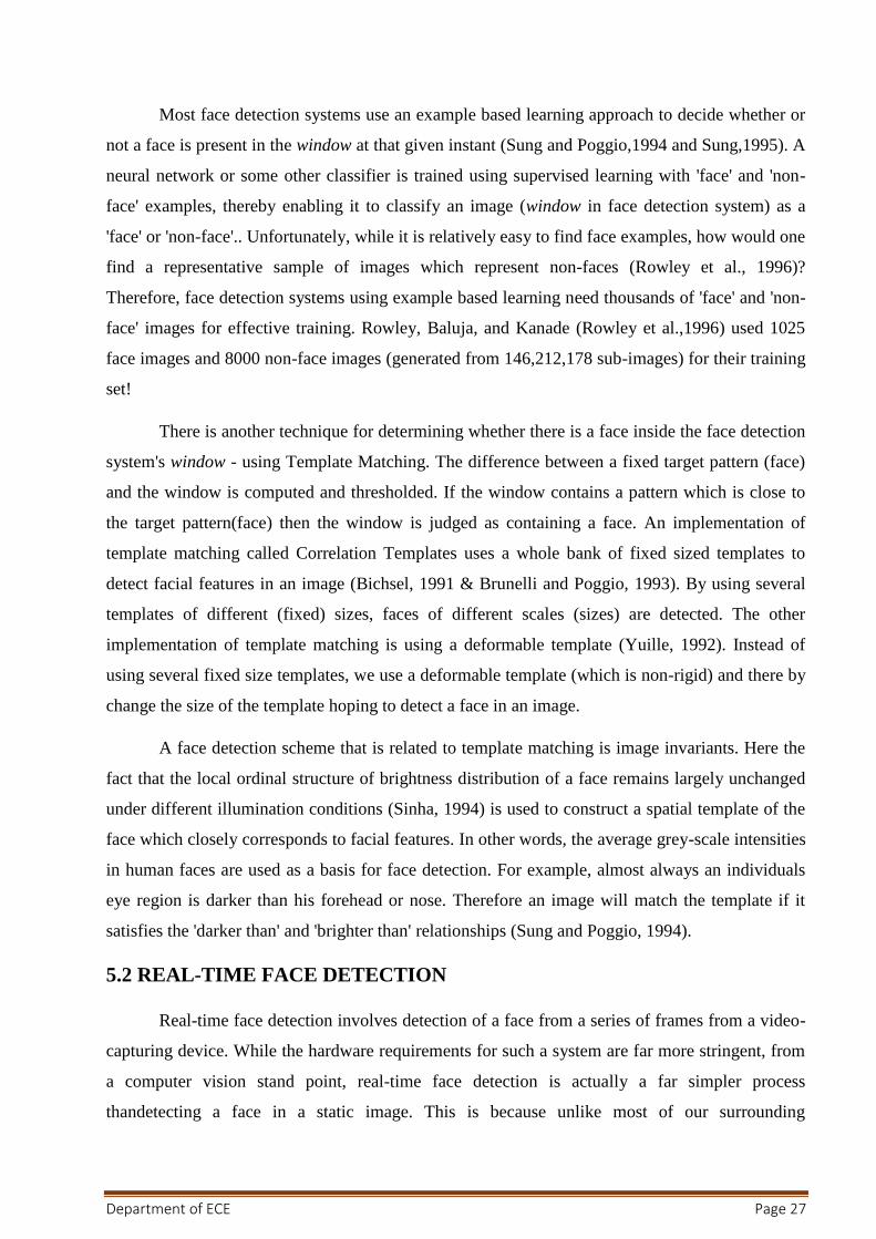
Most face detection systems use an example based learning approach to decide whether or

not a face is present in the window at that given instant (Sung and Poggio,1994 and Sung,1995). A

neural network or some other classifier is trained using supervised learning with 'face' and 'non-

face' examples, thereby enabling it to classify an image (window in face detection system) as a

'face' or 'non-face'.. Unfortunately, while it is relatively easy to find face examples, how would one

find a representative sample of images which represent non-faces (Rowley et al., 1996)?

Therefore, face detection systems using example based learning need thousands of 'face' and 'non-

face' images for effective training. Rowley, Baluja, and Kanade (Rowley et al.,1996) used 1025

face images and 8000 non-face images (generated from 146,212,178 sub-images) for their training

set!

There is another technique for determining whether there is a face inside the face detection

system's window - using Template Matching. The difference between a fixed target pattern (face)

and the window is computed and thresholded. If the window contains a pattern which is close to

the target pattern(face) then the window is judged as containing a face. An implementation of

template matching called Correlation Templates uses a whole bank of fixed sized templates to

detect facial features in an image (Bichsel, 1991 & Brunelli and Poggio, 1993). By using several

templates of different (fixed) sizes, faces of different scales (sizes) are detected. The other

implementation of template matching is using a deformable template (Yuille, 1992). Instead of

using several fixed size templates, we use a deformable template (which is non-rigid) and there by

change the size of the template hoping to detect a face in an image.

A face detection scheme that is related to template matching is image invariants. Here the

fact that the local ordinal structure of brightness distribution of a face remains largely unchanged

under different illumination conditions (Sinha, 1994) is used to construct a spatial template of the

face which closely corresponds to facial features. In other words, the average grey-scale intensities

in human faces are used as a basis for face detection. For example, almost always an individuals

eye region is darker than his forehead or nose. Therefore an image will match the template if it

satisfies the 'darker than' and 'brighter than' relationships (Sung and Poggio, 1994).

5.2 REAL-TIME FACE DETECTION

Real-time face detection involves detection of a face from a series of frames from a video-

capturing device. While the hardware requirements for such a system are far more stringent, from

a computer vision stand point, real-time face detection is actually a far simpler process

thandetecting a face in a static image. This is because unlike most of our surrounding


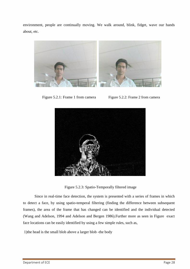
environment, people are continually moving. We walk around, blink, fidget, wave our hands

about, etc.

Figure 5.2.1: Frame 1 from camera Figure 5.2.2: Frame 2 from camera

Figure 5.2.3: Spatio-Temporally filtered image

Since in real-time face detection, the system is presented with a series of frames in which

to detect a face, by using spatio-temperal filtering (finding the difference between subsequent

frames), the area of the frame that has changed can be identified and the individual detected

(Wang and Adelson, 1994 and Adelson and Bergen 1986).Further more as seen in Figure exact

face locations can be easily identified by using a few simple rules, such as,

1)the head is the small blob above a larger blob -the body


2)head motion must be reasonably slow and contiguous -heads won't jump around erratically

(Turk and Pentland 1991a, 1991b).

Real-time face detection has therefore become a relatively simple problem and is possible

even in unstructured and uncontrolled environments using these very simple image processing

techniques and reasoning rules.

5.3 FACE DETECTION PROCESS

Fig 5.3 Face detection

It is process of identifying different parts of human faces like eyes, nose, mouth, etc… this

process can be achieved by using MATLAB codeIn this project the author will attempt to detect

faces in still images by using image invariants. To do this it would be useful to study the grey-

scale intensity distribution of an average human face. The following 'average human face' was

constructed from a sample of 30 frontal view human faces, of which 12 were from females and 18

from males. A suitably scaled colormap has been used to highlight grey-scale intensity

differences.

scaled colormap scaled colormap (negative)

Figure 5.3.1 Average human face in grey-scale


The grey-scale differences, which are invariant across all the sample faces are strikingly

apparent. The eye-eyebrow area seem to always contain dark intensity (low) gray-levels while

nose forehead and cheeks contain bright intensity (high) grey-levels. After a great deal of

experimentation, the researcher found that the following areas of the human face were suitable for

a face detection system based on image invariants and a deformable template.

scaled colormap scaled colormap (negative)

Figure 5.3.2 Area chosen for face detection (indicated on average human face in gray scale)

The above facial area performs well as a basis for a face template, probably because of the

clear divisions of the bright intensity invariant area by the dark intensity invariant regions. Once

this pixel area is located by the face detection system, any particular area required can be

segmented based on the proportions of the average human face After studying the above images it

was subjectively decided by the author to use the following as a basis for dark intensity sensitive

and bright intensity sensitive templates. Once these are located in a subject's face, a pixel area

33.3% (of the width of the square window) below this.

Figure 5.3.3: Basis for a bright intensity invariant sensitive template.

Note the slight differences which were made to the bright intensity invariant sensitive

template (compare Figures 3.4 and 3.2) which were needed because of the pre-processing done by


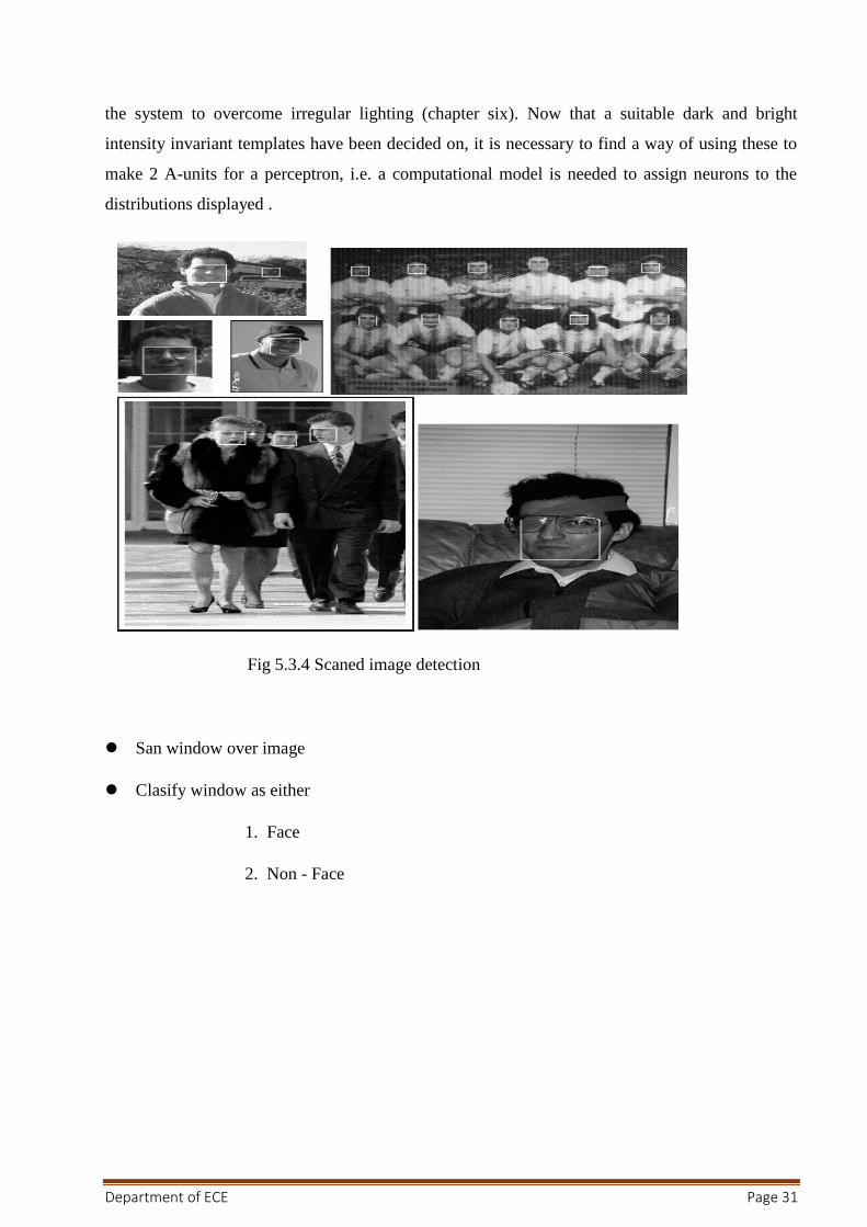
the system to overcome irregular lighting (chapter six). Now that a suitable dark and bright

intensity invariant templates have been decided on, it is necessary to find a way of using these to

make 2 A-units for a perceptron, i.e. a computational model is needed to assign neurons to the

distributions displayed .

Fig 5.3.4 Scaned image detection

San window over image

Clasify window as either

1. Face

2. Non - Face


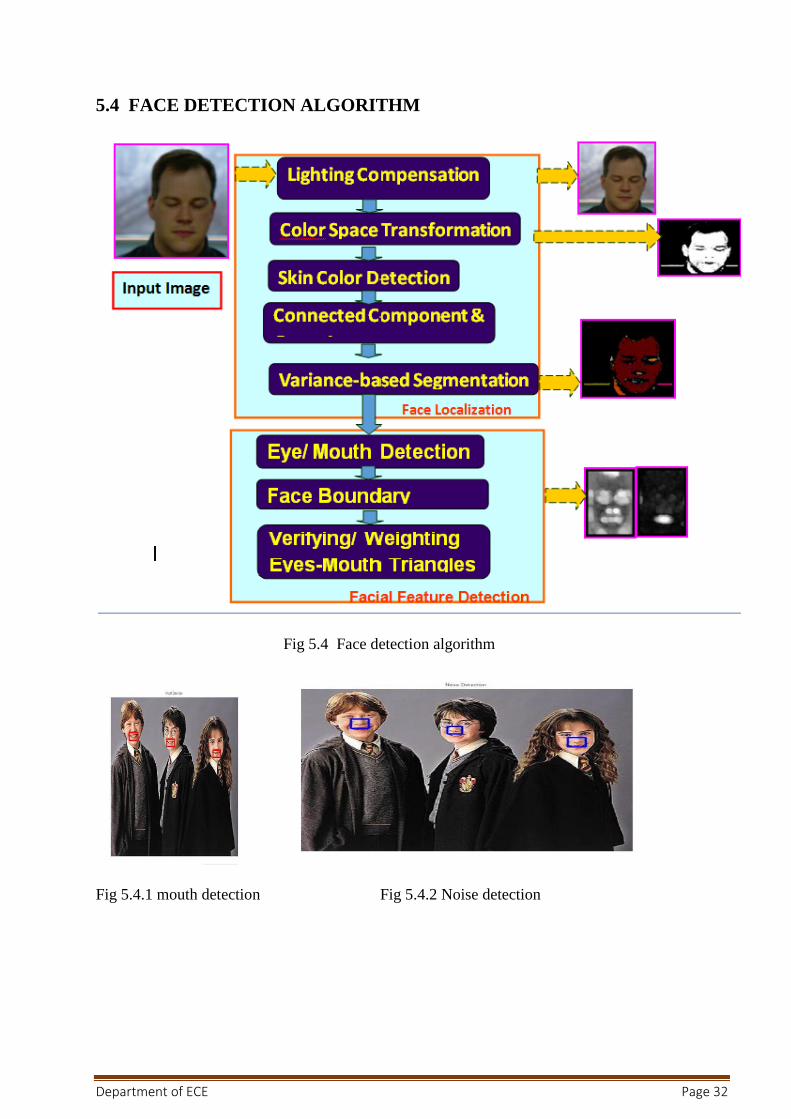
5.4 FACE DETECTION ALGORITHM

Fig 5.4 Face detection algorithm

Fig 5.4.1 mouth detection Fig 5.4.2 Noise detection


Fig 5.4.3 Eye detection


CHAPTER-6

FACE RECOGNITION

Over the last few decades many techniques have been proposed for face recognition. Many

of the techniques proposed during the early stages of computer vision cannot be considered

successful, but almost all of the recent approaches to the face recognition problem have been

creditable. According to the research by Brunelli and Poggio (1993) all approaches to human face

recognition can be divided into two strategies:

(1) Geometrical features and

(2) Template matching.

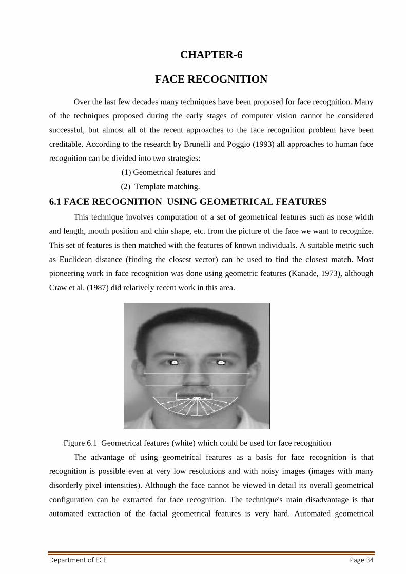
6.1 FACE RECOGNITION USING GEOMETRICAL FEATURES

This technique involves computation of a set of geometrical features such as nose width

and length, mouth position and chin shape, etc. from the picture of the face we want to recognize.

This set of features is then matched with the features of known individuals. A suitable metric such

as Euclidean distance (finding the closest vector) can be used to find the closest match. Most

pioneering work in face recognition was done using geometric features (Kanade, 1973), although

Craw et al. (1987) did relatively recent work in this area.

Figure 6.1 Geometrical features (white) which could be used for face recognition

The advantage of using geometrical features as a basis for face recognition is that

recognition is possible even at very low resolutions and with noisy images (images with many

disorderly pixel intensities). Although the face cannot be viewed in detail its overall geometrical

configuration can be extracted for face recognition. The technique's main disadvantage is that

automated extraction of the facial geometrical features is very hard. Automated geometrical


feature extraction based recognition is also very sensitive to the scaling and rotation of a face in

the image plane (Brunelli and Poggio, 1993). This is apparent when we examine Kanade's(1973)

results where he reported a recognition rate of between 45-75 % with a database of only 20 people.

However if these features are extracted manually as in Goldstein et al. (1971), and Kaya and

Kobayashi (1972) satisfactory results may be obtained.

6.1.1 Face recognition using template matching

This is similar the template matching technique used in face detection, except here we are

not trying to classify an image as a 'face' or 'non-face' but are trying to recognize a face.

Figure .6.11 Face recognition using template matching

Whole face, eyes, nose and mouth regions which could be used in a template matching

strategy.The basis of the template matching strategy is to extract whole facial regions (matrix of

pixels) and compare these with the stored images of known individuals. Once again Euclidean

distance can be used to find the closest match. The simple technique of comparing grey-scale

intensity values for face recognition was used by Baron (1981). However there are far more

sophisticated methods of template matching for face recognition. These involve extensive pre-

processing and transformation of the extracted grey-level intensity values. For example, Turk and

Pentland (1991a) used Principal Component Analysis, sometimes known as the eigenfaces

approach, to pre-process the gray-levels and Wiskott et al. (1997) used Elastic Graphs encoded

using Gabor filters to pre-process the extracted regions. An investigation of geometrical features

versus template matching for face recognition by Brunelli and Poggio (1993) came to the

conclusion that although a feature based strategy may offer higher recognition speed and smaller

memory requirements, template based techniques offer superior recognition accuracy.


6.2 PROBLEM SCOP AND SYSTEM SPECIFICATION

The following problem scope for this project was arrived at after reviewing the literature

on face detection and face recognition, and determining possible real-world situations where such

systems would be of use. The following system(s) requirements were identified

1 A system to detect frontal view faces in static images

2 A system to recognize a given frontal view face

3 Only expressionless, frontal view faces will be presented to the face detection&recognition

4 All implemented systems must display a high degree of lighting invariency.

5 All systems must posses near real-time performance.

6 Both fully automated and manual face detection must be supported

7 Frontal view face recognition will be realised using only a single known image

8 Automated face detection and recognition systems should be combined into a fully automated

face detection and recognition system. The face recognition sub-system must display a slight

degree of invariency to scaling and rotation errors in the segmented image extracted by the face

detection sub-system.

9 The frontal view face recognition system should be extended to a pose invariant face recognition

system.

Unfortunately although we may specify constricting conditions to our problem domain, it

may not be possible to strictly adhere to these conditions when implementing a system in the real-

world.

6.3 BRIEF OUT LINE OF THE IMPLEMENTED SYSTEM

Fully automated face detection of frontal view faces is implemented using a deformable

template algorithm relying on the image invariants of human faces. This was chosen because a

similar neural-network based face detection model would have needed far too much training data

to be implemented and would have used a great deal of computing time. The main difficulties in

implementing a deformable template based technique were the creation of the bright and dark

intensity sensitive templates and designing an efficient implementation of the detection algorithm.

Figure 6.3 Implemented fully automated frontal view face detection model


A manual face detection system was realised by measuring the facial proportions of the

average face, calculated from 30 test subjects. To detect a face, a human operator would identify

the locations of the subject's eyes in an image and using the proportions of the average face, the

system would segment an area from the image

A template matching based technique was implemented for face recognition. This was

because of its increased recognition accuracy when compared to geometrical features based

techniques and the fact that an automated geometrical features based technique would have

required complex feature detection pre-processing.

Of the many possible template matching techniques, Principal Component Analysis was

chosen because it has proved to be a highly robust in pattern recognition tasks and because it is

relatively simple to implement. The author would also liked to have implemented a technique

based on Elastic Graphs but could not find sufficient literature about the model to implement such

a system during the limited time available for this project.

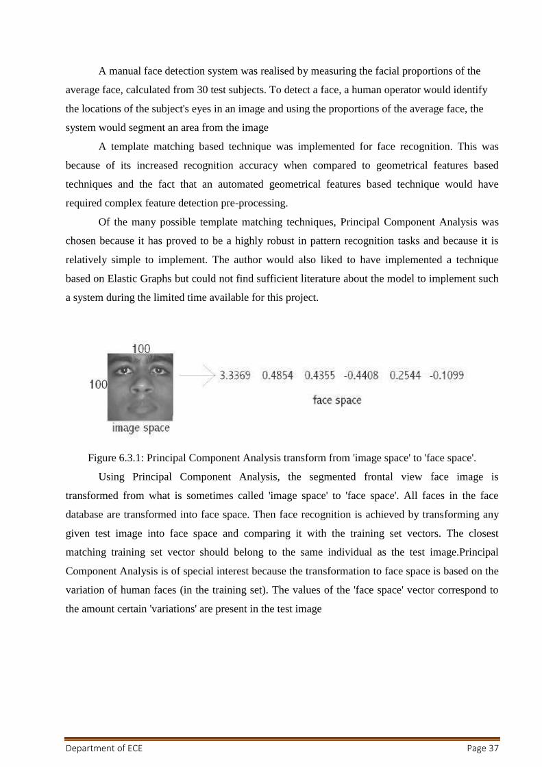
Figure 6.3.1: Principal Component Analysis transform from 'image space' to 'face space'.

Using Principal Component Analysis, the segmented frontal view face image is

transformed from what is sometimes called 'image space' to 'face space'. All faces in the face

database are transformed into face space. Then face recognition is achieved by transforming any

given test image into face space and comparing it with the training set vectors. The closest

matching training set vector should belong to the same individual as the test image.Principal

Component Analysis is of special interest because the transformation to face space is based on the

variation of human faces (in the training set). The values of the 'face space' vector correspond to

the amount certain 'variations' are present in the test image


Face recognition and detection system is a pattern recognition approach for personal

identification purposes in addition to other biometric approaches such as fingerprint recognition,

signature, retina and so forth. Face is the most common biometric used by humans applications

ranges from static, mug-shot verification in a cluttered background.

Fig 6.3.2 Face Recognition

6.4 FACE RECOGNITION DIFFICULTIES

1. Identify similar faces (inter-class similarity)

2. Accommodate intra-class variability due to

2.1 head pose

2.2 illumination conditions

2.3 expressions

2.4 facial accessories

2.5 aging effects

3. Cartoon faces


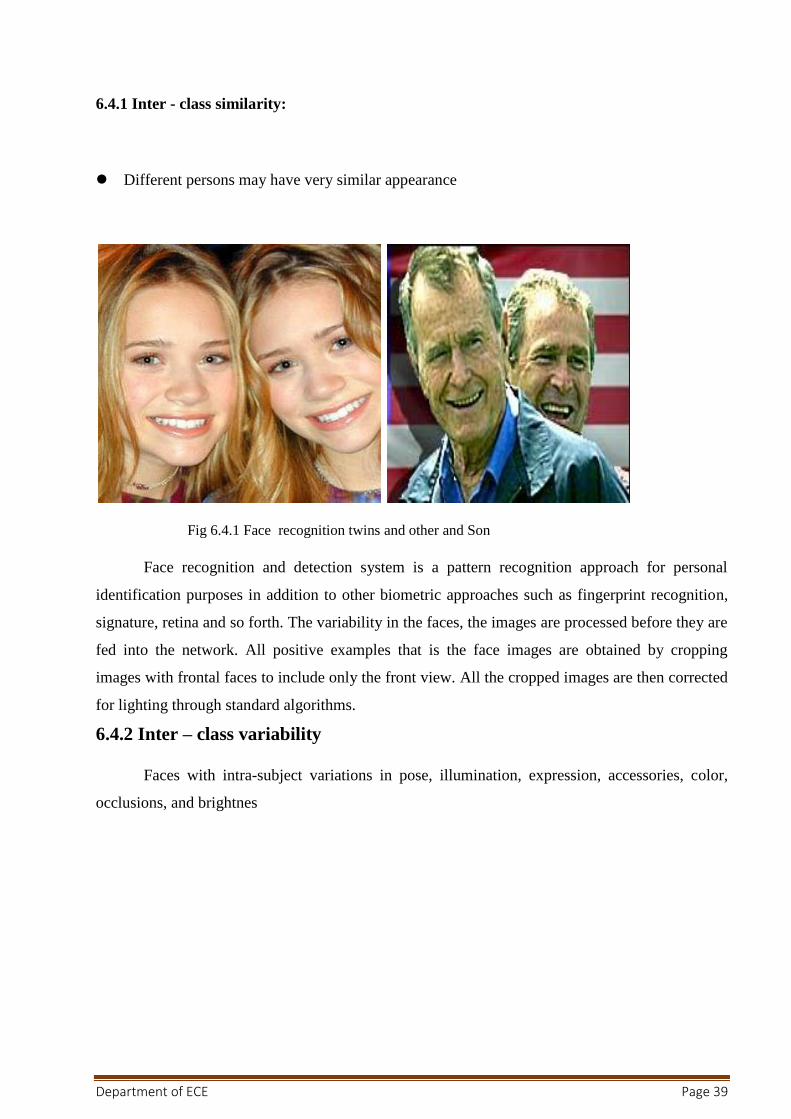
6.4.1 Inter - class similarity:

Different persons may have very similar appearance

Fig 6.4.1 Face recognition twins and other and Son

Face recognition and detection system is a pattern recognition approach for personal

identification purposes in addition to other biometric approaches such as fingerprint recognition,

signature, retina and so forth. The variability in the faces, the images are processed before they are

fed into the network. All positive examples that is the face images are obtained by cropping

images with frontal faces to include only the front view. All the cropped images are then corrected

for lighting through standard algorithms.

6.4.2 Inter – class variability

Faces with intra-subject variations in pose, illumination, expression, accessories, color,

occlusions, and brightnes


6.5 PRINCIPAL COMPONENT ANALYSIS (PCA)

Principal Component Analysis (or Karhunen-Loeve expansion) is a suitable strategy for

face recognition because it identifies variability between human faces, which may not be

immediately obvious. Principal Component Analysis (hereafter PCA) does not attempt to

categorise faces using familiar geometrical differences, such as nose length or eyebrow width.

Instead, a set of human faces is analysed using PCA to determine which 'variables' account for the

variance of faces. In face recognition, these variables are called eigen faces because when plotted

they display an eerie resemblance to human faces. Although PCA is used extensively in statistical

analysis, the pattern recognition community started to use PCA for classification only relatively

recently. As described by Johnson and Wichern (1992), 'principal component analysis is

concerned with explaining the variance- covariance structure through a few linear combinations of

the original variables.' Perhaps PCA's greatest strengths are in its ability for data reduction and

interpretation. For example a 100x100 pixel area containing a face can be very accurately

represented by just 40 eigen values. Each eigen value describes the magnitude of each eigen face

in each image. Furthermore, all interpretation (i.e. recognition) operations can now be done using

just the 40 eigen values to represent a face instead of the manipulating the 10000 values contained

in a 100x100 image. Not only is this computationally less demanding but the fact that the

recognition information of several thousand.

6.6 UNDERSTANDING EIGENFACES

Any grey scale face image I(x,y) consisting of a NxN array of intensity values may also be

consider as a vector of N2. For example, a typical 100x100 image used in this thesis will have to

be transformed into a 10000 dimension vector!

Figure 6.6.0 A 7x7 face image transformed into a 49 dimension vector

This vector can also be regarded as a point in 10000 dimension space. Therefore, all the

images of subjects' whose faces are to be recognized can be regarded as points in 10000 dimension


space. Face recognition using these images is doomed to failure because all human face images are

quite similar to one another so all associated vectors are very close to each other in the 10000-

dimension space.

Fig 6.6.1 Eigenfaces

The transformation of a face from image space (I) to face space (f) involves just a simple

matrix multiplication. If the average face image is A and U contains the (previously calculated)

eigenfaces,

f = U * (I - A)

This is done to all the face images in the face database (database with known faces) and to

the image (face of the subject) which must be recognized. The possible results when projecting a

face into face space are given in the following figure.

.


There are four possibilities:

1. Projected image is a face and is transformed near a face in the face database

2.Projected image is a face and is not transformed near a face in the face database

3.Projected image is not a face and is transformed near a face in the face database

4. Projected image is not a face and is not transformed near a face in the face database

While it is possible to find the closest known face to the transformed image face

by calculating the Euclidean distance to the other vectors, how does one know whether the image

that is being transformed actually contains a face? Since PCA is a many-to-one transform, several

vectors in the image space (images) will map to a point in face space (the problem is that even

non-face images may transform near a known face image's faces space vector). Turk and Pentland

(1991a), described a simple way of checking whether an image is actually of a face. This is by

transforming an image into face space and then transforming it back (reconstructing) into image

space. Using the previous notation,

I' = UT

*U * (I - A

With these calculations it is possible to verify that an image is of a face and recognise

that face. O'Toole et al. (1993) did some interesting work on the importance of eigen faces with

large and small eigenvalues. They showed that the eigen vectors with larger eigenvalues convey

information relative to the basic shape and structure of the faces. This kind of information is

most useful in categorising faces according to sex, race etc. Eigen vectors with smaller

eigenvalues tend to capture information that is specific to single or small subsets of learned

faces and are useful for distinguishing a particular face from any other face. Turk and Pentland

(1991a) showed that about 40 eigen faces were sufficient for a very good description of human

faces since the reconstructed image have only about 2% RMS. pixel-by-pixel errors.


0.8235

0.0661

-0.8786

-0.4727

-0.0646

0.6642

-0.4840

-0.4501

-0.2506

0.1591

0.3359

0.0048

0.0745

………..

Hippo in image space Hippo in face space Reconstructed hippo in image space

0.7253

-0.0392

0.2896

-0.1725

-0.2642

-0.0014

-0.0814

-0.0054

-0.0623

-0.0965

-0.0879

0.0745

-0.0261

…………

Face in image space Face in face space Reconstructed face in image space

Figure 6.6.3 Images and there reconstruction. The Euclidean distance between a face image and

its reconstruction will be lower than that of a non-face image


6.7 IMPROVING FACE DETECTION USING RECONSTRUCTIN

Reconstruction cannot be used as a means of face detection in images in near real-time

since it would involve resizing the face detection window area and large matrix multiplication,

both of which are computationally expensive. However, reconstruction can be used to verify

whether potential face locations identified by the deformable template algorithm actually contain a

face. If the reconstructed image differs greatly from the face detection window then the window

probably does not contain a face. Instead of just identifying a single potential face location, the

face detection algorithm can be modified to output many high 'faceness' locations which can be

verified using reconstruction. This is especially useful because occasionally the best 'faceness'

location found by the deformable template algorithm may not contain the ideal frontal view face

pixel area.

Output from Face detection system

Heuristic x y width

978 74 31 60

1872 74 33 60

1994 75 32 58

2125 76 32 56

2418 76 34 56

2389 79 32 50

2388 80 33 48

2622 81 33 46

2732 82 32 44

Best heuristic location (94,65,20) 2936 84 33 40

2822 85 58 38

2804 86 60 36

2903 86 62 36

3311 89 62 30

3373 91 63 26

3260 92 64 24

3305 93 64 22

3393 94 65 20


potential face locations that have been identified by the face detection system (the best face

locations it found on its search) are checked whether they contain a face. If the threshold level

(maximum difference between reconstruction and original for the original to be a face) is set

correctly this will be an efficient way to detect a face. The deformable template algorithm is fast

and can reduce the search space of potential face locations to a handful of positions. These are

then checked using reconstruction. The number of locations found by the face detection system

can be changed by getting it to output, not just the best face locations it has found so far but any

location, which has a 'faceness' value, which for example is, at least 0.9 times the best heuristic

value that has been found so far. Then there will be many more potential face locations to be

checked using reconstruction. This and similar speed versus accuracy trade-off decisions have to

be made keeping in mind the platform on which the system is implemented.

Similarly, instead of using reconstruction to check the face detection system's output, the output's

correlation with the average face can be checked. The segmented areas with a high correlation

probably contains a face. Once again a threshold value will have to be established to classify faces

from non-faces. Similar to reconstruction, resizing the segmented area and calculating its

correlation with the average face is far too expensive to be used alone for face detection but is

suitable for verifying the output of the face detection system.

6.8 POSE INVARIANT FACE RECOGNITION

Extending the frontal view face recognition system to a pose-invariant recognition system

is quite simple if one of the proposed specifications of the face recognition system is relaxed.

Successful pose-invariant recognition will be possible if many images of a known individual are in

the face database. Nine images from each known individual can be taken as shown below. Then if

an image of the same individual is submitted within a 30o angle from the frontal view he or she

can be identified.

Nine images in face database from a single known individual


Unknown image from same individual to be identified

Fig: 6.8 Pose invariant face recognition.

Pose invariant face recognition highlights the generalisation ability of PCA. For example,

when an individual's frontal view and 30o left view known, even the individual's 15

o left view can

be recognised


CONCLUSION

The computational models, which were implemented in this project, were chosen after

extensive research, and the successful testing results confirm that the choices made by the

researcher were reliable.The system with manual face detection and automatic face recognition did

not have a recognition accuracy over 90%, due to the limited number of eigenfaces that were used

for the PCA transform. This system was tested under very robust conditions in this experimental

study and it is envisaged that real-world performance will be far more accurate.The fully

automated frontal view face detection system displayed virtually perfect accuracy and in the

researcher's opinion further work need not be conducted in this area.

The fully automated face detection and recognition system was not robust enough to

achieve a high recognition accuracy. The only reason for this was the face recognition subsystem

did not display even a slight degree of invariance to scale, rotation or shift errors of the segmented

face image. This was one of the system requirements identified in section 2.3. However, if some

sort of further processing, such as an eye detection technique, was implemented to further

normalise the segmented face image, performance will increase to levels comparable to the

manual face detection and recognition system. Implementing an eye detection technique would be

a minor extension to the implemented system and would not require a great deal of additional

research.All other implemented systems displayed commendable results and reflect well on the

deformable template and Principal Component Analysis strategies.The most suitable real-world

applications for face detection and recognition systems are for mugshot matching and surveillance.

There are better techniques such as iris or retina recognition and face recognition using the thermal

spectrum for user access and user verification applications since these need a very high degree of

accuracy.The real-time automated pose invariant face detection and recognition system proposed

in chapter seven would be ideal for crowd surveillance applications. If such a system were widely

implemented its potential for locating and tracking suspects for law enforcement agencies is

immense.

The implemented fully automated face detection and recognition system (with an eye

detection system) could be used for simple surveillance applications such as ATM user security,

while the implemented manual face detection and automated recognition system is ideal of

mugshot matching. Since controlled conditions are present when mugshots are gathered, the

frontal view face recognition scheme should display a recognition accuracy far better than the

results, which were obtained in this study, which was conducted under adverse conditions.


Furthermore, many of the test subjects did not present an expressionless, frontal view to

the system. They would probably be more compliant when a 6'5'' policeman is taking their

mugshot! In mugshot matching applications, perfect recognition accuracy or an exact match is not

a requirement. If a face recognition system can reduce the number of images that a human

operator has to search through for a match from 10000 to even a 100, it would be of incredible

practical use in law enforcement.

The automated vision systems implemented in this thesis did not even approach the

performance, nor were they as robust as a human's innate face recognition system. However, they

give an insight into what the future may hold in computer vision.


REFERANCE

• Adelson, E. H., and Bergen, J. R. (1986) The Extraction of Spatio-Temporal Energy in

• Human and Machine Vision, Proceedings of Workshop on Motion: Representation and

• Analysis (pp. 151-155) Charleston, SC; May 7-9

• AAFPRS(1997). A newsletter from the American Academy of Facial Plastic and

Reconstructive Surgery. Third Quarter 1997, Vol. 11, No. 3. Page 3.

• Baron, R. J. (1981). Mechanisms of human facial recognition. International Journal of Man

Machine Studies, 15:137-178

• Beymer, D. and Poggio, T. (1995) Face Recognition From One Example View, A.I. Memo

No. 1536, C.B.C.L. Paper No. 121. MIT

• Bichsel, M. (1991). Strategies of Robust Objects Recognition for Automatic Identification

of Human Faces. PhD thesis, , Eidgenossischen Technischen Hochschule, Zurich.

• Brennan, S. E. (1982) The caricature generator. M.S. Thesis. MIT.

• Brunelli, R. and Poggio, T. (1993), Face Recognition: Features versus Templates. IEEE

Transactions on Pattern Analysis and Machine Intelligence, 15(10):1042-1052

• Craw, I., Ellis, H., and Lishman, J.R. (1987). Automatic extraction of face features. Pattern

Recognition Letters, 5:183-187, February.

• Deffenbacher K.A., Johanson J., and O'Toole A.J. (1998) Facial ageing, attractiveness, and

distinctiveness. Perception. 27(10):1233-1243

• Dunteman, G.H. (1989) Principal Component Analysis. Sage Publications.

• Frank, H. and Althoen, S. (1994). Statistics: Concepts and applications. Cambridge

University Press. p.110

• Gauthier, I., Behrmann, M. and Tarr, M. (1999). Can face recognition really be

dissociated from object recognition? Journal of Cognitive Neuroscience, in press.

• Goldstein, A.J., Harmon, L.D., and Lesk, A.B. (1971). Identification of human faces.

In Proc. IEEE, Vol. 59, page 748

• de Haan, M., Johnson, M.H. and Maurer D. (1998) Recognition of individual faces

and average face prototypes by 1- and 3- month-old infants. Centre for Brain and

Cognitive

• Development, Department of Psychology, Birkbeck College.

• Hadamard, J. (1923) Lectures on the Cauchy Problem in Linear Partial Differential

Equations , Yale University Press


• Haralick, R.M. and Shapiro, L.G.. (1992) Computer and Robot Vision, Volume I.

Addison-Wesley

• Haxby, J.V., Ungerleider, L.G., Horwitz, B., Maisog, J.M., Rapoport, S.I., and Grady,

C.L. (1996). Face encoding and recognition in the human brain. Proc. Nat. Acad. Sci.

93: 922 - 927.

• Heisele, B. and Poggio, T. (1999) Face Detection. Artificial Intelligence Laboratory.

MIT.

• Jang., J., Sun, C., and Mizutani, E. (1997) Neuro-Fuzzy and Soft Computing. Prentice

Hall.

• Johnson, R.A., and Wichern, D.W. (1992) Applied Multivariate Statistical Analysis.

Prentice Hall. p356-395


APPENDIX

FACE DETECTION:

clear all

clc

%Detect objects using Viola-Jones Algorithm

%To detect Face

FDetect = vision.CascadeObjectDetector;

%Read the input image

I = imread('HarryPotter.jpg');

%Returns Bounding Box values based on number of objects

BB = step(FDetect,I);

figure,

imshow(I); hold on

for i = 1:size(BB,1)

rectangle('Position',BB(i,:),'LineWidth',5,'LineStyle','-

','EdgeColor','r');

end

title('Face Detection');

hold off;

The step(Detector,I) returns Bounding Box value that contains

[x,y,Height,Width] of the objects of interest.

BB =

52 38 73 73

379 84 71 71

198 57 72 72


NOSE DETECTION:

%To detect Nose

NoseDetect = vision.CascadeObjectDetector('Nose','MergeThreshold',16);

BB=step(NoseDetect,I);

figure,

imshow(I); hold on



','EdgeColor','b');

end

title('Nose Detection');

hold off;

EXPLANATION:

To denote the object of interest as 'nose', the argument 'Nose' is

passed.

vision.CascadeObjectDetector('Nose','MergeThreshold',16);

The default syntax for Nose detection :

vision.CascadeObjectDetector('Nose');

Based on the input image, we can modify the default values of the

parameters passed to vision.CascaseObjectDetector. Here the default

value for 'MergeThreshold' is 4.

When default value for 'MergeThreshold' is used, the result is not

correct.

Here there are more than one detection on Hermione.

To avoid multiple detection around an object, the 'MergeThreshold'

value can be overridden.


MOUTH DETECTION:

%To detect Mouth

MouthDetect = vision.CascadeObjectDetector('Mouth','MergeThreshold',16);

BB=step(MouthDetect,I);

figure,

imshow(I); hold on



','EdgeColor','r');

end

title('Mouth Detection');

hold off;

EYE DETECTION:

%To detect Eyes

EyeDetect = vision.CascadeObjectDetector('EyePairBig');

%Read the input Image

I = imread('harry_potter.jpg');

BB=step(EyeDetect,I);

figure,imshow(I);

rectangle('Position',BB,'LineWidth',4,'LineStyle','-','EdgeColor','b');

title('Eyes Detection');

Eyes=imcrop(I,BB);

figure,imshow(Eyes);


FACE RECOGNITION

function closeness=recognition(input_image,U,R);

% By L.S. Balasuriya

% Returns closeness of known face vectors in R to unknown image

input_image % R contains the Eigenfaces

%********image to vector ***********************************************

vinput=reshape(input,[10000 1]);

%********recognition **************************************************

facespace=voutput'*U;

%********Eucleadian distance ******************************************

[p,ignor]=size(R);

distance_vecs=R-repmat(facespace,[p 1]);

distance=sum(abs(distance_vecs)')';

%********order of closeness to unknown face ***************************

[ignor,closeness]=sort(distance);

a project report on face recognition …pace.ac.in/documents/ece/face recognition system with...a...

Documents