A PROJECT TO INVESTIGATE THE EFFECT OF MASONRY INFILL ON THE

BEHAVIOR OF THE STRUCTURE IN ASEISMIC PRONE AREA.

A FINAL YEAR PROJECT REPORT SUBMITTED TO KAMPALA INTERNATIONAL

UNIVERSITY IN PARTIAL FULFILLMENT OF THE AWARD OF BACHELOR OF

SCIENCE IN CIVIL ENGINEERING

BY

THEMBO ALFRED 1153-03104-03107

and

OLIVIA TABAN GEORGE BSCE/40595/143/DF

DEPARTMENT OF CIVIL ENGINEERING

SCHOOL OF ENGINEERING AND APPLIED SCIENCES

SEPTEMBER 2019

i

DECLARATION

We declare that the information contained herein is to best of our Knowledge true in reference to

the three months we undertook in designing the project. Hence no part of this report unless or

otherwise referenced has been presented to this school or any other institution for the same or

related cause.

NAME REGISTRATION NUMBER SIGNATURE

1. THEMBO ALFRED 1153-03104-03107 …………………………

2. TIBAN OLIVIA GEORGE BSCE/40595/143/DF …………………………

ii

APPROVAL

I humbly declare that this project Report has been prepared under my supervision.

Supervisor’s name MR. BARUGAHARE RAYMOND

Signature……………………………………………

Date………………………………………………………

iii

ACKNOWLEDGEMENT

First and foremost, we would like to thank the almighty God for the wisdom, support, good

health and protection He accorded to us. Special thanks go to our project supervisor MR.

RAYMOND, whose constructive advice and inspiration has enabled us to come up with this

project report.

iv

TABLE OF CONTENTS

DECLARATION ...................................................................................................................... i

APPROVAL ............................................................................................................................ ii

ACKNOWLEDGEMENT ...................................................................................................... iii

TABLE OF CONTENTS ....................................................................................................... iv

LIST OF FIGURES ................................................................................................................ vi

LIST OF TABLES................................................................................................................ viii

ABSTRACT ........................................................................................................................... ix

CHAPTER ONE ...................................................................................................................... 1

INTRODUCTION: .................................................................................................................. 1

1.1 BACKGROUND: .............................................................................................................. 1

1.2 PROBLEM STATEMENT ............................................................................................... 7

1.3 MAIN OBJECTIVE: ......................................................................................................... 8

1.4 SCOPE ............................................................................................................................... 8

1.5 LIMITATION OF BOVE THE PROJECT ...................................................................... 9

1.6 SIGNIFICANCE OF THE PROJECT ............................................................................. 10

1.7 JUSTIFICATION ............................................................................................................ 10

CHAPTER TWO ................................................................................................................... 11

LITERATURE REVIEW ...................................................................................................... 11

CHAPTER THREE ............................................................................................................... 21

METHODOLOGY ................................................................................................................ 21

3.0. INTRODUCTION .......................................................................................................... 21

3.1 MODELING OF MASONRY ......................................................................................... 21

3.2 LINEAR SEISMIC ANALYSIS ..................................................................................... 23

3.3 EQUIVALENT LATERAL FORCE METHOD ............................................................ 27

3.4 MODAL RESPONSE SPECTRUM ANALYSIS ........................................................... 29

3.5 NONLINEAR SEISMIC ANALYSIS ............................................................................ 29

3.5.1 STEPS FOR MODELING AND STATIC ANALYSIS, ............................................. 29

v

3.6 PUSHOVER ANALYSIS ............................................................................................... 36

CHAPTER FOUR ................................................................................................................. 41

RESULTS AND DISCUSSION ............................................................................................ 41

4.1 MODELLING OF MATERIAL PROPERTIES ............................................................. 41

CHAPTER FIVE : RECOMMENDATIONS AND CONCLUSSION ................................. 99

5.1 CONCLUSSION ............................................................................................................. 99

5.2 RECOMMNDATION ................................................................................................... 101

REFERENCES .................................................................................................................... 102

APPENDIX ......................................................................................................................... 103

vi

LIST OF FIGURES

Figure 1:. Restriction to the lateral displacement of a column creating a captive-column effect. 11

Figure 2. Typical captive-column failure. ..................................................................................... 11

Figure 3:. Captive-Column Failure in an RC Frame at Lefkada (Greece),2003 Earthquake

(Karakostas et al. 2005) ................................................................................................................ 12

Figure 4:. Lateral forces and shear forces generated in buildings due to ground motion ............. 13

Figure 5. Distribution of total displacement generated by an earthquake in: (a) a regular building;

and (b) a building with soft story irregularity. .............................................................................. 13

Figure 6: Damage of Izmit earthquake (Adapazarı) ..................................................................... 14

Figure 7: Damage to soft storey of Izmit Earthquake (Yalova-Gölcük). ..................................... 14

Figure 8. Observed effects of interaction between infills and bare frame: a) shear failure of

column and b) exterior joint shear damage (Bolero, Molise 2002); c) global collapse for soft

storey mechanism (Izmit, 1999). .................................................................................................. 15

Figure 9:. Failure mechanisms of the infilled frames observed in the experiments conducted by:

(a) Al-Char at. al (2005) ;(b) Stavrakis (2009); (c) Mehrabian (1994); (d) Blacked et. al (2009).

....................................................................................................................................................... 17

Figure 10. Failure mechanisms of infilled frames (Mehrabian, 1994) ......................................... 17

Figure 11: Different failure modes of the infilled frames: (a) corner crushing; (b) sliding shear;

(c) diagonal compression; (d) diagonal cracking; and (e) frame bending failure (El-Lakhani et al.,

2003) as shown in the figure above. ............................................................................................. 18

Figure 12. Schematic force-displacement response of the infill strut model proposed by Seined

and Hobbs (1995). ......................................................................................................................... 18

Figure 13. Schematic force-displacement response of the infill strut model proposed by Doles

and Fanfares (2008). ..................................................................................................................... 19

Figure 14:. Left: corner column; center: Arnold, Ch. (1982) and V. Bergeron (1997); right:

(Photos: V. Berger). ...................................................................................................................... 19

Figure 15. Different crack patterns for the URM piers ................................................................. 20

Figure 16: model with masonry .................................................................................................... 22

Figure 17: Stress- strain curve of concrete according to mander .................................................. 22

Figure 18: Stress stain curve of steel according to park ............................................................... 23

Figure 19: The stress strain curve of concrete according to mander ............................................ 41

Figure 20: Stress-strain curve for steel ......................................................................................... 41

Figure 21: Section for design moment .......................................................................................... 42

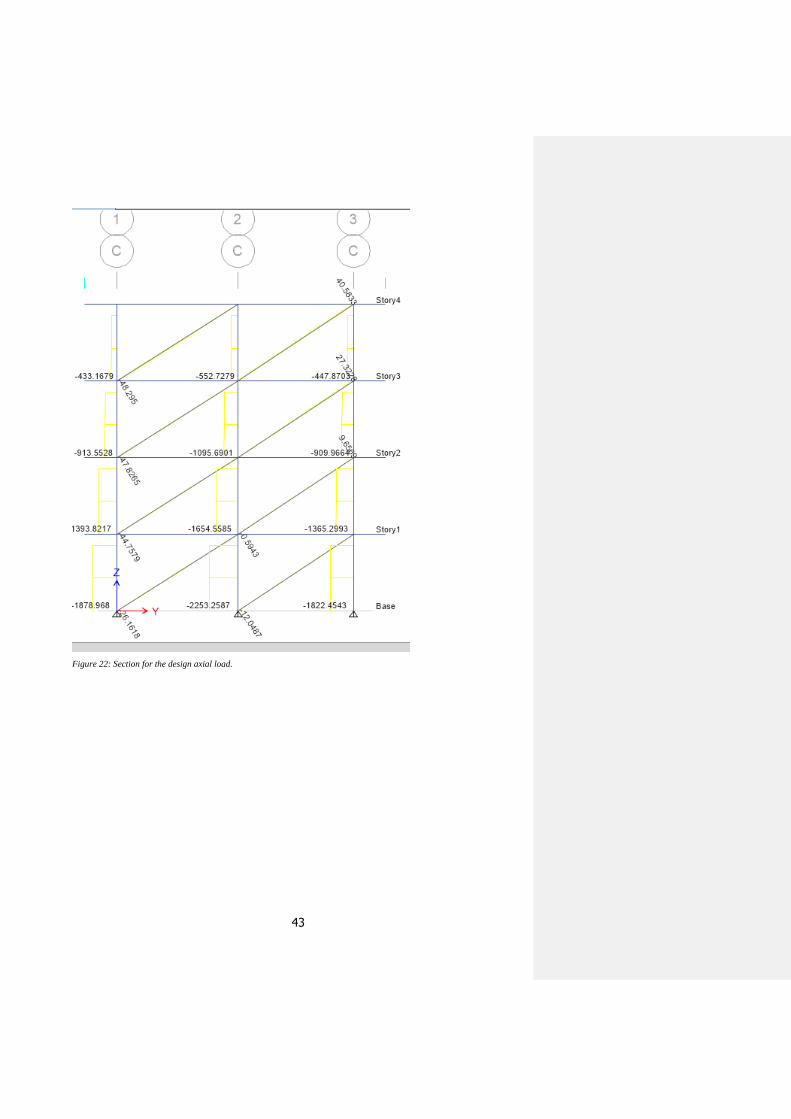
Figure 22: Section for the design axial load. ................................................................................ 43

Figure 23: The design section for shear ........................................................................................ 44

Figure 24: The design section was obtained as;............................................................................ 45

Figure 25: The design section for the moment ............................................................................. 46

Figure 26: The design section for axial force. .............................................................................. 46

Figure 27: The design section for shear. ....................................................................................... 47

Figure 28: Deformed shapes. ........................................................................................................ 50

vii

Figure 29: Push Y ......................................................................................................................... 51

Figure 30: A graph for inter- storey drifts for push x ................................................................... 53

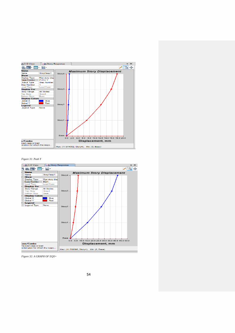
Figure 31: Push Y ......................................................................................................................... 54

Figure 32: A GRAPH OF EQX+ .................................................................................................. 54

Figure 33: A graph of EQY+ ........................................................................................................ 55

Figure 34: The graph of the base shear against the displacements. .............................................. 59

Figure 35: For push x .................................................................................................................... 60

Figure 36: For push Y ................................................................................................................... 61

Figure 37: For push x .................................................................................................................... 69

Figure 38: The story drift increase with increase in number of models. The maximum story

drift=117922.395mm at story 5 .................................................................................................... 71

Figure 39: Base shear against monitored displacement ................................................................ 74

Figure 40MODELLINNG OF G+6 ............................................................................................ 103

Figure 41 DEFORMED SHAPE AFTRE PUSHOVER ............................................................. 104

viii

LIST OF TABLES

Table 1: The maximum design valves of the two variables are summarized below; ................... 48

Table 2: Modal load participation ratios ....................................................................................... 49

Table 3: Modal participating mass ratios ...................................................................................... 49

Table 4: For push x ....................................................................................................................... 53

Table 5: Story Response .............................................................................................................. 55

Table 6: Base Shear vs Monitored Displacement ..................................................................... 56

Table 7: FEMA 440 Equivalent Linearization .......................................................................... 57

Table 8: NTC 2008 Target Displacement .................................................................................. 57

Table 9: Base Shear vs Monitored Displacement ..................................................................... 62

Table 10: Time History Plot ........................................................................................................ 64

Table 11: Time History Plot ....................................................................................................... 64

Table 12: Story Max/Avg Displacements................................................................................... 65

Table 13: The modal periods and frequencies are summarized below ......................................... 67

Table 14: the story stiffness .......................................................................................................... 68

Table 15: Story Response ............................................................................................................ 71

Table 16: The base shear shar against the monitored displacements for push x .......................... 72

Table 17: Story Max/Avg Displacements................................................................................... 76

Table 18: The modal frequency and the periods were summarized as below .............................. 78

ix

ABSTRACT

This project carried out comparative seismic performance of reinforced concrete frames infilled

by masonry walls with different heights. Partial and fully infilled RC frames were modeled for

the research objectives and the analysis model for a bare reinforced concrete frame was

established for comparison. Non-linear static analyses for the studied frames were performed to

investigate their structural behavior under extreme loading conditions and to find out their

collapse mechanism. It was observed from analysis results that the strengths of the partial infilled

RC frames are increased and their ductility is reduced, as infilled masonry walls are higher.

Especially, reinforced concrete frames with a higher partial infilled masonry wall would

experience shear failures. Non-linear dynamic analyses using three earthquake records show that

the bare and fully infilled reinforced concrete frames present stable collapse mechanism while

the reinforced concrete frames with a partially infilled masonry wall collapse in more brittle

manner due to short-column effects.

1

CHAPTER ONE

INTRODUCTION:

1.1 BACKGROUND:

Theory of earthquakes:

An earthquake is the result of a sudden release of energy in the Earth's crust that creates

seismic waves. The elastic rebound theory is an explanation for how energy is spread during

earthquakes. As rocks on opposite sides of a fault are subjected to force and shift, they

accumulate stress energy and slowly deform (strain) until their internal strength is exceeded.

At that time, a sudden movement occurs along the fault, releasing the accumulated energy,

and the rocks snap back to their original un deformed shape. In geology, the elastic rebound

theory was the first theory to satisfactorily explain earthquakes. (Richter el al.,1994) [3].

During the earthquake, the portions of the rock around the fault that were locked and had not

moved 'spring' back, relieving the strain (accumulated over several years) in a few seconds.

Like an elastic band, the more the rocks are strained, the more elastic energy is stored and the

greater potential for an event. The stored energy is released during the rupture partly as heat,

partly in damaging the rock, and partly as elastic waves. Modern measurements using GPS

largely support Reid’s theory as the basis of seismic movement, though actual events are

often more complicated. (Reid, 2001) [9].

2

An earthquake's hypo-center is the position where the strain energy stored in the rock is first

released, marking the point where the fault begins to rupture. This occurs at the focal depth

below the epicenter. This is the point on the Earth's surface that is directly above the hypo-

center, the point where an earthquake originates.

FAULTS

Earthquakes occur along faults.

A fault is a planar fracture or discontinuity in a volume of rock, across which there has been

significant displacement. Large faults within the Earth's crust result from the action of

3

tectonic forces. Energy release associated with rapid movement on active faults is the cause

of most earthquakes.

There are three main types of faults:

A normal fault occurs when the crust is extended.

The hanging wall moves downward relative to the footwall.

A thrust fault occurs when the crust is compressed.

The hanging wall moves upward relative to the footwall.

The fault surface is usually near the vertical and motion results from shearing forces.

4

SEISMIC WAVES;

Seismic waves are waves of energy that travel through the earth’s layers, and are as a result

of earthquakes, volcanic eruptions, magma movements, large landslides and large man-made

explosions that give out low frequency acoustic energy.

There are two types of seismic waves, body wave and surface waves.

Body waves originate in the hypocenter and propagate spherically through the interior of the

Earth. They follow ray paths refracted by the varying density and modulus (stiffness) of the

Earth's interior. The density and modulus, in turn, vary according to temperature,

composition, and phase. There are two types of body waves: P-waves and S-waves.

Surface waves are analogous to water waves and travel along the Earth's surface. They travel

slower than body waves. Because of their low frequency, long duration, and large amplitude,

they can be the most destructive type of seismic wave. There are two types of surface waves:

Rayleigh waves and Love waves.

The P-wave, where P stands for Primary wave or Pressure wave, can travel through gases,

solids and liquids, including the Earth. It has the highest velocity (5-8 km/s during an

earthquake) and is therefore the first to be recorded, and it is formed from alternating

compressions and rarefactions. In isotropic and homogeneous solids, the polarization of a P-

wave is always longitudinal; thus, the particles in the solid have vibrations along (or parallel

to) the travel direction of the wave energy. (Harry Fielding Reid,1906) [5].

5

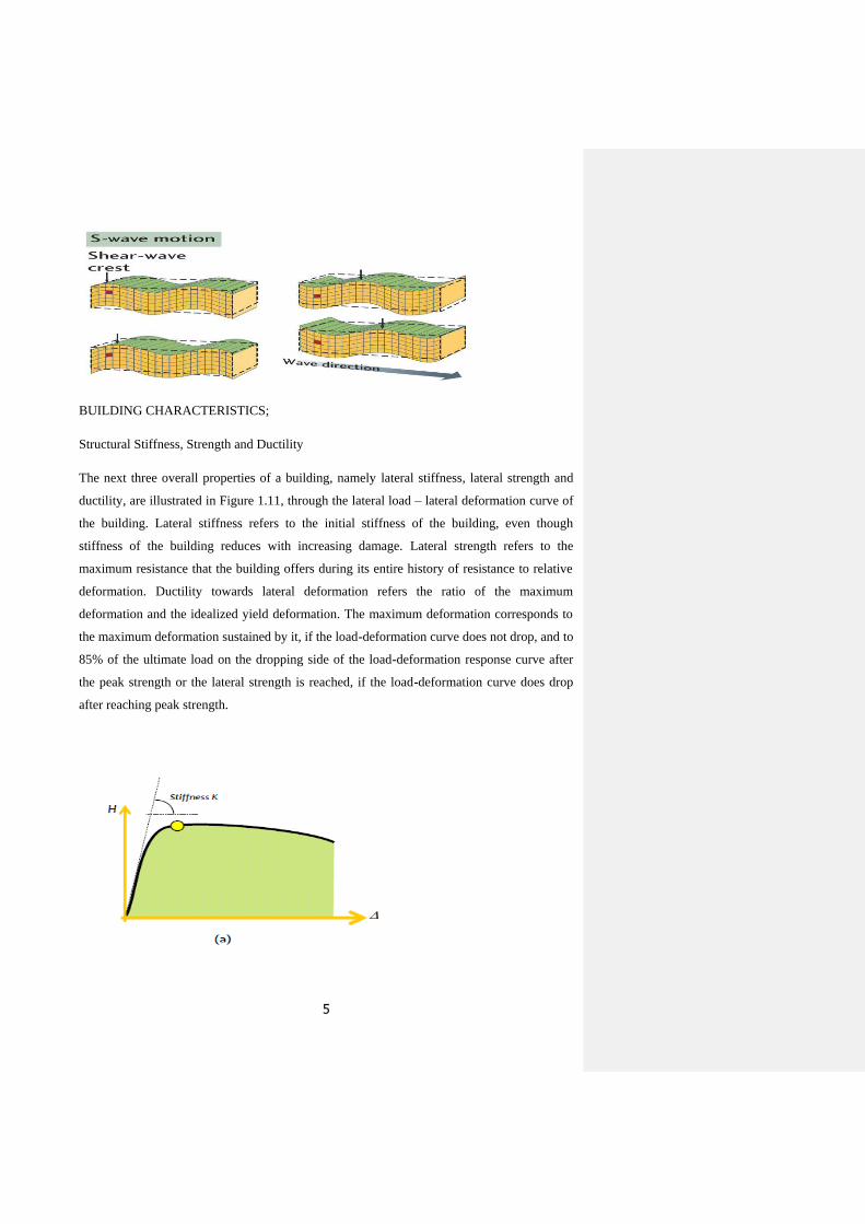
BUILDING CHARACTERISTICS;

Structural Stiffness, Strength and Ductility

The next three overall properties of a building, namely lateral stiffness, lateral strength and

ductility, are illustrated in Figure 1.11, through the lateral load – lateral deformation curve of

the building. Lateral stiffness refers to the initial stiffness of the building, even though

stiffness of the building reduces with increasing damage. Lateral strength refers to the

maximum resistance that the building offers during its entire history of resistance to relative

deformation. Ductility towards lateral deformation refers the ratio of the maximum

deformation and the idealized yield deformation. The maximum deformation corresponds to

the maximum deformation sustained by it, if the load-deformation curve does not drop, and to

85% of the ultimate load on the dropping side of the load-deformation response curve after

the peak strength or the lateral strength is reached, if the load-deformation curve does drop

after reaching peak strength.

6

Figure 1.11: Structural Characteristics: Overall load deformation curves of a building,

indicating (a) lateral stiffness, (b) lateral strength, and (c) ductility towards lateral

deformation

EARTHQUAKE DEMAND VERSUS EARTHQUAKE CAPACITY

The method of design of buildings should therefore take into account the deformation

demand on the building, and the deformation capacity of the building. The former depends on

the seismic-tectonic setting of the location of the building, but the latter is within the control

of the design professionals (i.e., architects and engineers). The concern is that both of these

quantities have uncertainties. On one hand, even though some understanding is available on

the maximum possible ground displacement at a location, earth scientists are not able to

clearly provide the upper bound for these numbers. Each new damaging earthquake has

7

always provided surprises. And, on the other hand, analytical tools are not available to

estimate precisely the overall nonlinear behavior of an as-built structure, and its ultimate

deformation capacity. (Goel, 2008) [11].

Figure 1.12: Double demand in Buildings subjected to earthquake effects: Need large

inelastic deformation capacity in the building and need to sustain the induced forces.

1.2 PROBLEM STATEMENT

The effect of infill walls on structural rigidity of whole structure are ignored despite the fact

that reinforced concrete frames with infill walls are the most commonly used building

systems. Analysis and calculation models including infill wall contribution are difficult and

complex especially on major construction projects. Behavior of masonry infilled R.C. frames

under seismic loads should be modeled to consider the effect of the infill walls on the seismic

performance of the structure. The gaps occurred between the frame elements (beam or

columns), the walls and the cracks on the walls are the most important parameters for

structural design if infill walls are considered as structural members.

8

Determination of the maximum load capacity and the behavior of the frames with infill walls

subjected to seismic forces are complex and questionable problems. Seismic response of infill

frames has been investigated for long both analytically and experimentally.

FEMA-306 identifies four possible failure modes for Masonry infill that also give an

indication of potential crack and damage patterns in Masonry infill. The failure modes are

sliding-shear failure, compression failure, diagonal tension cracking, and general shear

failure. In addition to these failure modes of masonry infill, RC frame may fail due to the

flexural failures of beams and columns due to yielding of tension steel, shear failure of beams

and columns, and shear failure and bond failure of beam-column joints.

1.3 MAIN OBJECTIVE:

To investigate the effect of masonry infill on the behavior of the structure.

Specific objectives:

This will be accomplished by the following specific objectives;

To assess the impact of masonry on the stiffness of the structure.

To assess the impact of masonry infill on the ductility of the structure.

To determine the effect of the transverse reinforcement spacing on the seismic behavior of

the structure.

1.4 SCOPE

GEOGRAPHICAL SCOPE

9

Figure 2. Seismic zoning of Uganda and the project area is FORT-PORTAL located in zone

one as shown on the map for seismic zoning in Uganda.

1.5 LIMITATION OF BOVE THE PROJECT

This research will be limited to investigate the seismic response of reinforced concrete (RC)

frame building considering the effect of modeling masonry infill (MI) walls. The seismic

behavior of a residential 5-storey RC frame building, considering and ignoring the effect of

10

masonry, will be numerically investigated using response spectrum (RS) analysis to improve

the structural on the structural integrity in Fort-Portal district in Kabarole Region as an

earthquake prone area in accordance to the Ugandan standard seismic code of practice for

structural design.

The methodology will be limited to The Equivalent diagonal strut method that will be used to

represent the behavior of infill walls, whilst the well-known software package ETABS will be

used for implementing all frame models and performing the analysis.

1.6 SIGNIFICANCE OF THE PROJECT

Its purpose will ensure, with adequate reliability, that in an event of earthquakes:

(i) Human lives are protected

(ii) Damages are limited

(ii) Critical facilities remain operational.

1.7 JUSTIFICATION

Developing construction techniques that are seismic resistant.

11

CHAPTER TWO

LITERATURE REVIEW

The captive-column effect is caused by a non-intended modification to the original structural

configuration of the column that restricts the ability of the column to deform laterally by

partially confining it with building components as a result of only a fraction of its height can

deform laterally, corresponding to the free portion; thus the term captive column. (Guevara

and Garcia 2005).

Figure 1:. Restriction to the lateral displacement of a column creating a captive-column effect.

Figure 2. Typical captive-column failure.

12

Figure 3:. Captive-Column Failure in an RC Frame at Lefkada (Greece),2003 Earthquake (Karakostas et al. 2005)

Davidovic (1999) [43], carried out an investigation about the effect of the soft storey on the

behavior of the structure and observed that during an earthquake, more moment and shear

strength fall on the columns and walls in the entrance floors than the one in the upper storeys.

This can be called dangerous storey instead of soft storey as shown in Figure 5 below.

(Guevara, 1989),also carried out the project on the soft storey and observed that the soft story

irregularity, refers to the existence of a building floor that presents a significantly lower

stiffness than the others due to unconscientiousness as a result of reduction in number of rigid

13

non-structural walls in one of the floors of a building. If the soft story effect is not foreseen

on the structural design, irreversible damage will generally be present on both the structural

and nonstructural components of that floor. This may cause the local collapse, and in some

cases even the total collapse of the building due to the displacement of the structure as shown

by the figure below.

Figure 4:. Lateral forces and shear forces generated in buildings due to ground motion

Figure 5. Distribution of total displacement generated by an earthquake in: (a) a regular building; and (b) a building with

soft story irregularity.

14

Figure 6: Damage of Izmit earthquake (Adapazarı)

Figure 7: Damage to soft storey of Izmit Earthquake (Yalova-Gölcük).

Sozen, M.A., et al (1968, p. 39), carried out a project on the Failure modes of soft storey and

in his project observed failure mechanism of the buildings which failed during earthquakes in

recent years indicate that the existing buildings that are most vulnerable to damage and

collapse from earthquake excitation in low and moderate seismicity regions are the soft

storied buildings, i.e. those buildings that possess storeys that are significantly weaker or

15

more flexible than adjacent story and where deformations and damage tend to be

concentrated.

Magenes and Stefano Pampanin (2004, p.144), carried out a project on the presence of infills

(e.g. typically un-reinforced masonry) and observed that they can lead to unexpected and

controversial effects due to the interaction with the bare frame.

Figure 8. Observed effects of interaction between infills and bare frame: a) shear failure of column and b) exterior joint

shear damage (Bolero, Molise 2002); c) global collapse for soft storey mechanism (Izmit, 1999).

Basing on the above idea will be adopted and applied to the investigation of the effect of

infills to the behavior of the structure in Formal-portal.

(Li et al., 2008; Seen et al., 2003)[7],carried out an investigation on the failure Modes of

infilled RC Frames and made from Observations of past earthquakes (including 1999 Kocal,

Turkey earthquake, the 2008 Sichuan, China earthquake, and the 1999 Chi-Chi, Taiwan

Earthquake) show severe damage to these types of structures, as illustrated in Figure 11.

Damage patterns include partial or full failure of masonry panels, shear failure of columns,

column plastic hinges, soft story mechanisms, short column shear failures.

16

Figure 12. Different failure mechanisms in: (a) Algeria (2003 Boomers Earthquake), masonry

wall failure (photo: S. Breve); (b) India (2001 Bhuj earthquake), (photo: EERI, 2001); (c)

Taiwan, (1999 Chi-Chi earthquake) (photo: Charleston, 2008).Mehrabian and Stavrakis

(2009)[10],carried out a project on failure modes of masonry frames and observed that failure

mechanisms of the masonry infilled frames are complex because of the high number of

parameters involved in the seismic response of the structure such as the material property,

configuration, relative stiffness of the frame to the infill, detailing, etc. and outlined some of

the failure mechanism as follows;

(i) Diagonal cracking in the infill with column shear failure or, more rarely, plastic hinges in

columns. This failure typically occurs in weak/non-ductile frames with strong infill;

(ii) Horizontal sliding of the masonry with flexural or shear failure of the columns. Infill

crushing is sometimes observed in these tests. This failure mechanism was observed in the

weak frames with weak panels and also in the strong and ductile frames with weak infill

panels;

(iii) Infill corner crushing with flexural failure in the columns. This mechanism is most likely

in strong and ductile frames with strong infill.

17

Figure 9:. Failure mechanisms of the infilled frames observed in the experiments conducted by: (a) Al-Char at. al (2005)

;(b) Stavrakis (2009); (c) Mehrabian (1994); (d) Blacked et. al (2009).

Figure 10. Failure mechanisms of infilled frames (Mehrabian, 1994)

Similarly, (El-Lakhani et al., 2003)[9] categorized the failure mechanisms of masonry infilled

frames into five distinct modes, illustrated in Figure 2-4: (a) corner crushing failure, which is

associated with strong frame with weak infill (similar to failure mode (iii) above), (b) sliding

shear failure, associated with weak mortar joint infill bounded with strong frame (same as

failure mode (ii), above), (c) diagonal compression failure, associated with slender flexible

infill walls, (d) diagonal cracking failure, associated with weak frame with relatively strong

18

infill (similar to failure mode (i) above), and e) a frame bending failure mode which is

associated with weak frame with weak infill.

Figure 11: Different failure modes of the infilled frames: (a) corner crushing; (b) sliding shear; (c) diagonal compression;

(d) diagonal cracking; and (e) frame bending failure (El-Lakhani et al., 2003) as shown in the figure above.

Basing on the above idea, it will be adopted and applied to investigate the effect of masonry

infill on the behavior of the structure in a seismic prone area of Formal-Portal.

After Klingler and Barter (1976) considered the nonlinear behavior of the infill panel in the

dynamic response, Seined and Hobbs (1995) also tried to predict the nonlinear behavior of

the infill panel. They modified the equivalent diagonal strut model to consider the nonlinear

behavior of the infill, to account for its low ductility, cracking and crushing load as well

varying response due to differences in the infill such as aspect ratio and beam to column

strength/stiffness ratio. This bilinear model predicts the initial stiffness (KN), cracking load

(FCRA), crushing load (Fax), stiffness and displacement (cap) at the peak load, as shown in

Figure 15-16. However, they did not define the post-peak response of the infill

Figure 12. Schematic force-displacement response of the infill strut model proposed by Seined and Hobbs (1995).

19

Figure 13. Schematic force-displacement response of the infill strut model proposed by Doles and Fanfares (2008).

Francisco Restfully et.al (2004, p.4), carried out an investigation about the effects of the

torsion on the building and observed that Torsional effects may significantly modify the

seismic response of buildings, and they have caused severe damage or collapse of structures

in several past earthquakes. These effects occur due to different reasons, such as no uniform

distribution of the mass, stiffness and strength, torsional components of the ground

movement, etc. as shown in the figure 15.

Figure 14:. Left: corner column; center: Arnold, Ch. (1982) and V. Bergeron (1997); right: (Photos: V. Berger).

These experiments described in FEMA 307 have shown that URM piers can have

considerable deformability and ductility if certain failure mechanisms prevail. Axial stress,

aspect ratio, boundary conditions, and relative strength between mortar joints and units

determine the failure mechanisms of masonry piers. FEMA 273 (ATC 1997) gives four

typical crack patterns and failure modes for the URM piers as shown in Figure 17.

20

(a) Rocking (b) Sliding (c) Diagonal tension (d) Toe crushing

Figure 15. Different crack patterns for the URM piers

Basing on the above idea shall be adopted and applied to investigate the effect of infills on

the behavior of the structure in seismic prone area in Formal-portal.

21

CHAPTER THREE

METHODOLOGY

3.0. INTRODUCTION

Etab is the primary FEM analysis and design tool for any type of project including towers,

culverts, plants, bridges, stadium and marine structures. With an array of advanced analysis

capabilities including linear static, response spectra, time history, cable and push over and

non-linear analysis, Etab provides good compatibility with a scalable solution that will meet

the demands of project every time hence the project has been realized through the following

steps in pertinent to ETABS.

3.1 MODELING OF MASONRY

The MI walls were usually modeled as equivalent diagonal compression strut as shown in

figure bellow. In this method the infill wall has been idealized as diagonal strut and the frame

was modelled as truss element. FEMA-306 recommends the following equations, which are

based on the early studies to calculate the properties of diagonal compression strut where the

area Ae as a function of the width of the strut we and the thickness of the infill panel t being:

The width of the strut in terms of the height of the panel h and panel length l can be expressed

as:

where the value of can be calculated as;

where Ec and Em respectively denote the elastic moduli of the column and the

masonry wall, is the angle defining diagonal strut inclination Ic is the moment of inertia of

the column and Hw is the height of the infill wall.

The masonry was modelled as the diagonal struct.

Length=4.830 m

Width=5.02 m

Thickness=0.25 m

Commented [T1]:

22

Figure 16: model with masonry

And then the material properties were modeled according to mander and park to obtain the

stress-strain curves of concrete and steel respectively.

Figure 17: Stress- strain curve of concrete according to mander

23

Figure 18: Stress stain curve of steel according to park

3.2 LINEAR SEISMIC ANALYSIS

The linear analysis of the two variants (with and without masonry) of G+4 building was

achieved through the following steps.

Step - 1: Initial setup of Standard Codes and the Ugandan standard seismic code for earth

quake analysis was adopted as below with Display in metric units by clicking file and a new

model was chosen:

Step - 2: Creation of Grid points & Generation of structure.

24

The grid points were created and edited as shown below in the dialogue box

The window dialogue box appears and then chose the Custom Grid Spacing and edit the

grids.

This was done by entering the grid dimensions and storey dimensions of the building.

Step - 3: Defining of Material property.

Material Properties were defined after which New Materials were added this was successfully

achieved by selecting the define menu material properties of which new material for our

structural components such as the beams, columns and slabs were specified by giving them

specified properties as illustrate below.

25

Step –4: Defining the Frame Sections.

After defining the property, structural components such as the beams, columns and slabs

were defined by selecting frame sections and the required sections were added.

26

Step - 5: Slab Details

This was achieved by selecting the section properties and the slab properties were defined as

below

Step - 6: Assigning of Property.

27

Step - 7: Defining of loads

The loads in ETABS were defined as static load cases.

Step - 8: Assigning of Supports

By keeping the selection at the base of the structure and selecting all the columns, supports

were assigned by going to assign menu joint or frame Restraints (supports).

Step - 9: Assigning Loads

Slab load were assigned as shell loads and applied to the___14 selected shell area as

demonstrated below.

The frame load finishes were assigned to the frame through selecting the frame area and were

distributed evening.

3.3 EQUIVALENT LATERAL FORCE METHOD

This was achieved by modelling the structure until the structure was free from the geometry

and torsional irregularities. This was justified as below.

28

In accordace to the above modelling, the mass participation ratios in the static and dynamic

analysis was 100% hence this meets the standards of Eurocode 8.

Then the Equivalent Lateral Force Method was adopted to the model.

29

3.4 MODAL RESPONSE SPECTRUM ANALYSIS

This was performed in Etab to estimate the peak value of the seismic action. This was

achieved though applying the seismic loads in the horizontal directions, X and Y for the

determination of natural frequencies and vibrations

3.5 NONLINEAR SEISMIC ANALYSIS

The analysis of nonlinear seismic analysis in ETABS 17 involved the following four steps

namely, Designing and Pushover analysis.

The pushover analysis was applied on the two variables (with and without

masonry) with varying height namely G+4, G+5, G+6, G+7 and G+8.

3.5.1 STEPS FOR MODELING AND STATIC ANALYSIS,

Creating the models

The basic grid system was created. The structural objects were set relative to the grid system.

the grid system was created by clicking the File menu and New model was chosen, as

displayed. The Grid dimension, Story dimension and Units were as well displayed.

30

The appropriate Design code were selected for reinforce concrete frame design.

Then the material properties were defined by clicking on the define tool and the material

property command was selected.

Defining the section properties;

The various section properties used in the model were defined by clicking the Define menu

and then Frame Section command, the form shown in below was displayed. the Add

31

Rectangular button was selected displaying the dialogue box in which add Section Name,

Dimensions, and Material were defined.

Defining of slab properties;

This was achieved by clicking the Define menu > Wall/Slab Sections command, the form

below was displayed. Slab was modified by the Modify/show section thereby Adding new

slab type and Geometry.

32

Drawing the Beam, Column and Slab

Beam

The beam was added to the grid system by selecting the draw quick beam command and then

its property of 300*450 was selected and then applied

Column

33

Then the column was added to the grid system using the quick draw column command and

the properties of the column were selected from the dialogue box and then applied.

Slab

The slab was added by clicking on quick draw floor command and the properties of the slab

were selected and then applied

Defining the Static load case;

The static load case was added by clicking the Define menu through the Static Load Cases

command button, and then the load cases were defined and modified in the dialogue box

34

Assigning the Structural Loads

The load cases were assigned by Clicking on the Assign menu and the shell area was chosen

and the load was applied as Uniformly distributed as displayed below.

Defining the Analysis option

To Define analysis option, Analysis menu > Set Analysis Option command was selected. The

Analysis was performed successfully and the results like deformations, shear forces, bending

moments of each element were displayed for each load cases and load combinations cases as

defined in the Display menu.

35

Designing the structure

The reinforced concrete frame was designed in Etab 17 by specifying the

reinforcements of each frame element through selecting the Concrete Frame Design and then

frame was Checked before running the analysis.

36

3.6 PUSHOVER ANALYSIS

Define hinge properties

Frame nonlinear properties were used to define nonlinear force-displacement and moment

rotation behavior that was assigned to discrete locations along the length of frame elements.

These nonlinear hinges were used during static nonlinear analysis. For all other types of

analysis, these hinges were rigid and had no effect on the linear behavior of element. The user

defined auto-plastic hinges were assigned to the frame elements. Then each element

automatically received the user defined plastic hinges. These hinges properties were pertinent

to ATC-40 and FEMA 273 and this was successfully done through the following steps.

Assigning the hinge properties:

The load patterns were defined

Then function response spectrum was defined

The load cases were defined the plastic hinges were assigned to each elect by clicking on the

define menu and then select the frame and chose the hinges and apply them to each frame

element as displayed below. After the assignment of the hinge properties to each frame

element and the pushover analysis was run.

Assignment of the hinge properties to the beam is justified by the dialogue box below.

37

Assignment of the hinges on the column is justified as below.

38

Assignment of the hinges to masonry is justified as below.

39

The above assignments are all justified by the diagram below

40

41

CHAPTER FOUR

RESULTS AND DISCUSSION

4.1 MODELLING OF MATERIAL PROPERTIES

Figure 19: The stress strain curve of concrete according to mander

The compressive strength of concrete was determined from the curve as 25N/mm^2 that was

equivalent to the compressive strength that concrete would achieve after 28 days.

Figure 20: Stress-strain curve for steel

42

The tensile strength of steel was determined from the graph as 460N/mm^2

The stress strain curve of steel that corresponded with the tensile strength of TMT500C as

adopted.

Linear analysis of G+4 with masonry

This was justified by;

Figure 21: Section for design moment

43

Figure 22: Section for the design axial load.

44

Figure 23: The design section for shear

The model without masonry (bare model)

This was justified by;

45

Figure 24: The design section was obtained as;

46

Figure 25: The design section for the moment

Figure 26: The design section for axial force.

47

Figure 27: The design section for shear.

48

Table 1: The maximum design valves of the two variables are summarized below;

reference Maximum design

valve

units combination

ETABS 17

Model of G+4 with

masonry

Moment 3-3=84.9811 KN.m ULS

Shear=90.0000 KN ULS

Stiffness=944184.264 KN/m

Base

sheear=30248.7263

KN EQY+MAX

Axial loads= 2253.5870 KN

Model of G+4 without

masonry

Moment 3-3=45.4737 KN.m

Shear=46.3339 KN

Stiffness=145313.96 KN/m

Base

sheear=15759.9798

KN EQX+ Max

Axial load=1275.6042 KN ULS

In accordance to the above results, it was observed that the model with masonry was more

rigid than the bare model. This due to the fact that masonry infills increases the base shear

when subjected to the earthquake loads as justified by the table above.

49

Table 2: Modal load participation ratios

Table 3: Modal participating mass ratios

The mass participation ratio was equal to 100% as demonstrated in the table 2.8 above and

this is in consideration to the Eurocode 8.

This is justified by participation of one modal mass in each direction in consideration to

EURODE 8 standards.

The sizes of the section of the frame were designed and the reinforcements are summarized in

the table below.

The above reinforcements were used in performing the pushover analysis.

This is justified by the following results.

50

Figure 28: Deformed shapes.

Push x

51

Figure 29: Push Y

52

In both cases, the masonry collapsed at the initial push due effect of increased inertial loads

due to earthquake loads.

The columns were damaged before the beam which indicates that there was a weak column to

the beam due to concentration of almost an entire mass of the building.

53

Story drifts

Table 4: For push x

Story Elevation Location X-Dir Y-Dir

m mm mm

Story4 12 Top 16.314 0.877

Story3 9 Top 14.614 0.826

Story2 6 Top 11.396 0.687

Story1 3 Top 6.714 0.437

Base

0 Top 0 0

This was justified by;

Figure 30: A graph for inter- storey drifts for push x

54

Figure 31: Push Y

Figure 32: A GRAPH OF EQX+

55

Figure 33: A graph of EQY+

The maximum drifts of the load case were summarized in the table below

Table 5: Story Response

Story Elevation Location X-Dir Y-Dir

LOAD

CASE

m mm mm

Story4 12 Top 41.508 6.913

PUSH

X

Story3 9 Top 4.769 54.315

PUSH

Y

56

Story2 6 Top 4.769 54.315 EQX+

Story1 3 Top 4.769 54.315 EQY+

Base 0 Top 3.584 34.85 Modal

The above chart indicated that the inter-storey drifts of G+4 with masonry increases with

increase of the modal mass.

Thus, the maximum storey drift in x-direction=41.508mm and in the y-direction=54.315mm

The static pushover results of G+4 with masonry were obtained as justified in the table below

Table 6: Base Shear vs Monitored Displacement

Step

Monitored

Dispel Base Force A-B B-C C-D D-E >E A-IO IO-LS

LS-

CP

mm KN

0 0 0 1021 0 0 0 0 986 34 1

1 -17.24 6380.8453 960 4 0 0 57 938 23 0

2 -65.327 23735.4736 667 294 0 0 60 934 23 4

3 -115.011 41833.8912 540 418 0 0 63 933 21 1

4 -164.004 59743.8423 493 462 0 0 66 932 22 1

5 -213.93 78094.1037 437 518 0 0 66 932 21 2

6 -265.258 96935.9963 426 528 0 0 67 932 19 2

7 -313.258 114581.2372 406 548 0 0 67 932 19 0

8 -361.258 132224.4456 395 558 0 0 68 932 19 0

57

9 -409.258 149868.6732 393 558 0 0 70 932 19 0

10 -457.258 167512.6812 391 560 0 0 70 931 20 0

11 -480 175872.1782 385 566 0 0 70 931 20 0

The maximum base shaer increased as the number of multiple steps increases as well as the

monitored displacements.

The maximum displacement was obtained as 480mm and the maximum base

shear=175872.1782KN.

Table 7: FEMA 440 Equivalent Linearization

Sd Sa Period

mm g sec

0 0 0

15.758 0.463796 0.37

59.508 1.71706 0.374

105.044 3.044425 0.373

149.912 4.355415 0.372

195.544 5.689757 0.372

242.502 7.063435 0.372

286.369 8.346165 0.372

330.235 9.628753 0.372

374.102 10.911422 0.372

417.968 12.194072 0.371

438.752 12.801774 0.371

According to FEMA the displacement increased as the period increases of which the period

may reach that of the ground hence indicating resonance.

The target displacement

Table 8: NTC 2008 Target Displacement

Sd Sa Period

mm g sec

0 0 0

58

15.758 0.463796 0.37

59.71 1.71706 0.374

105.121 3.044425 0.373

149.901 4.355415 0.372

195.534 5.689757 0.372

242.448 7.063435 0.372

286.321 8.346165 0.372

330.193 9.628753 0.372

374.066 10.911422 0.371

417.938 12.194072 0.371

438.724 12.801774 0.371

The maximum target displacement=438.724mm and occurred at the maximum period of

0.371 seconds.

These results were justified by the following pushover curves

59

Figure 34: The graph of the base shear against the displacements.

The graph slopes negatively due to the fact that the base shear increased down the story as

masonry infills increased more base down the story.

60

Figure 35: For push x

61

Figure 36: For push Y

There was no performance point on the pushover curve due to the overestimation of the

spectral acceleration of Ugandan standard seismic code for earthquake analysis in relation to

other international standard codes.

62

For the push Y

Table 9: Base Shear vs Monitored Displacement

Step

Monitored

Dispel Base Force A-B

B-

C C-D

D-

E >E A-IO IO-LS LS-CP >CP Total

mm KN

0 0 0 1021 0 0 0 0 986 34 1 0 1021

1 -0.099 5303.8132 971 2 0 0 48 949 22 2 48 1021

2 -1.82 -3505.5255 968 4 0 0 49 930 35 6 50 1021

3 -2.101 -6239.2244 965 6 0 0 50 929 30 12 50 1021

4 -2.137 -4292.2458 963 8 0 0 50 927 31 13 50 1021

5 -2.225 -5171.4471 961 10 0 0 50 926 32 11 52 1021

6 -2.246 -4069.0695 959 12 0 0 50 926 31 11 53 1021

7 -2.259 -4136.8601 959 12 0 0 50 926 31 11 53 1021

8 -2.295 -2207.9654 957 14 0 0 50 926 30 11 54 1021

9 -2.424 -5865.2144 955 16 0 0 50 926 28 11 56 1021

10 -2.454 -4245.8893 953 18 0 0 50 926 28 11 56 1021

11 -2.457 -4323.6302 953 18 0 0 50 926 28 11 56 1021

12 -2.64 5639.2018 936 30 0 0 55 926 24 10 61 1021

13 -2.868 6757.9597 930 32 0 0 59 926 23 10 62 1021

14 -2.923 7366.3305 925 34 0 0 62 926 22 9 64 1021

15 -2.944 7747.1137 921 38 0 0 62 926 22 9 64 1021

16 -2.947 8004.9803 915 44 0 0 62 926 22 9 64 1021

17 -3.008 8334.0127 913 46 0 0 62 925 23 8 65 1021

18 -3.014 8697.2747 911 48 0 0 62 925 23 8 65 1021

19 -3.028 8909.9478 907 52 0 0 62 925 23 8 65 1021

20 -3.053 9101.5085 901 58 0 0 62 925 23 8 65 1021

21 -3.084 9213.5731 899 60 0 0 62 925 23 8 65 1021

22 -3.092 9683.6713 893 64 0 0 64 925 23 8 65 1021

23 -3.13 10424.586 878 78 0 0 65 925 23 8 65 1021

24 -3.133 10590.1445 872 84 0 0 65 925 23 8 65 1021

25 -3.145 11060.9939 864 92 0 0 65 925 23 8 65 1021

26 -3.156 11568.2857 856 100 0 0 65 925 23 7 66 1021

27 -3.163 11720.1839 854 102 0 0 65 925 23 7 66 1021

28 -3.166 11896.5597 848 108 0 0 65 925 23 7 66 1021

29 -3.181 12416.521 836 120 0 0 65 925 23 7 66 1021

30 -3.203 13598.4856 818 138 0 0 65 925 23 7 66 1021

31 -3.214 13827.661 806 150 0 0 65 925 23 7 66 1021

32 -3.218 13992.1028 800 156 0 0 65 925 23 7 66 1021

33 -3.233 14200.3451 794 162 0 0 65 925 23 7 66 1021

63

34 -3.239 14487.3571 786 170 0 0 65 925 23 7 66 1021

35 -3.256 14701.26 780 176 0 0 65 925 23 7 66 1021

36 -3.269 14981.1078 774 182 0 0 65 925 23 7 66 1021

37 -3.282 15464.9965 766 190 0 0 65 925 23 7 66 1021

38 -3.334 18240.709 731 224 0 0 66 925 22 8 66 1021

39 -3.364 19024.3109 725 230 0 0 66 925 22 8 66 1021

40 -3.382 19734.7927 711 244 0 0 66 925 22 8 66 1021

41 -3.399 20659.2702 705 250 0 0 66 925 22 8 66 1021

42 -3.402 20889.4096 699 256 0 0 66 925 22 8 66 1021

43 -3.41 21314.5745 695 260 0 0 66 925 22 8 66 1021

44 -3.413 21603.2568 693 262 0 0 66 925 22 8 66 1021

45 -3.417 21802.2701 687 268 0 0 66 925 22 8 66 1021

46 -3.418 22088.2876 681 274 0 0 66 925 22 8 66 1021

47 -3.496 23372.5419 677 278 0 0 66 925 22 8 66 1021

48 -3.502 23657.3154 669 286 0 0 66 925 22 8 66 1021

49 -3.504 24086.0792 659 296 0 0 66 925 22 8 66 1021

50 -3.538 25966.5298 639 316 0 0 66 925 22 8 66 1021

51 -3.726 23192.9231 638 316 0 0 67 925 22 6 68 1021

52 -3.802 27196.0551 628 326 0 0 67 925 22 6 68 1021

53 -3.825 27931.2385 624 330 0 0 67 925 22 6 68 1021

54 -3.837 25266.0169 624 330 0 0 67 924 23 6 68 1021

55 -3.919 29333.105 614 340 0 0 67 924 23 6 68 1021

56 -3.942 29841.0772 612 342 0 0 67 924 23 5 69 1021

57 -3.966 30173.5993 610 344 0 0 67 924 23 5 69 1021

58 -3.983 30979.6381 604 350 0 0 67 924 23 5 69 1021

59 -3.989 31506.2477 594 360 0 0 67 924 23 5 69 1021

60 -3.995 31417.0669 594 360 0 0 67 924 23 5 69 1021

61 -4.007 32036.5826 592 362 0 0 67 924 23 5 69 1021

62 -4.03 32611.2393 588 366 0 0 67 924 23 5 69 1021

63 -4.054 33836.2573 581 372 0 0 68 924 23 5 69 1021

64 -4.124 36238.7544 573 380 0 0 68 924 23 5 69 1021

65 -4.171 38722.5133 561 392 0 0 68 924 23 5 69 1021

This shows that the bae shear in the y-direction increases as the numbers of steps increases.

the maximum base shear=38722.51333KN and occurred at the step 65

Time history plots for push

64

Table 10: Time History Plot

Step Base FX

KN

0 0

1 6239.8846

2 23211.1277

3 40909.7289

4 58424.027

5 76368.9084

6 94794.5603

7 112049.9959

8 129303.444

9 146557.8889

10 163812.1189

11 171986.9442

Time history for push x

This justified by the graph below

Table 11: Time History Plot

Step Base FX

KN

0 0

1 6239.8846

2 23211.1277

3 40909.7289

4 58424.027

5 76368.9084

6 94794.5603

7 112049.9959

8 129303.444

9 146557.8889

10 163812.1189

11 171986.9442

The above data is summarized on the graph below

65

The time history for push y =0.

The maximum displacement of the storey

Table 12: Story Max/Avg Displacements

Story Load Case/Combo Direction Maximum Average Ratio

mm mm

Story4 Dead X 0.937 0.931 1.006

Story4 Dead Y 0.823 0.81 1.017

Story3 Dead X 0.845 0.841 1.005

Story3 Dead Y 0.75 0.74 1.014

Story2 Dead X 0.667 0.664 1.004

Story2 Dead Y 0.598 0.592 1.011

Story1 Dead X 0.407 0.405 1.003

Story1 Dead Y 0.369 0.366 1.009

Story4 Live X 0.142 0.141 1.009

Story4 Live Y 0.121 0.118 1.025

Story3 Live X 0.127 0.126 1.007

Story3 Live Y 0.109 0.107 1.02

Story2 Live X 0.099 0.099 1.006

66

Story2 Live Y 0.087 0.085 1.016

Story1 Live X 0.059 0.059 1.005

Story1 Live Y 0.053 0.052 1.012

Story4 EQX+ Max X 41.12 39.81 1.033

Story4 EQX+ Max Y 6.913 5.021 1.377

Story3 EQX+ Max X 36.019 34.823 1.034

Story3 EQX+ Max Y 6.073 4.387 1.384

Story2 EQX+ Max X 26.889 25.947 1.036

Story2 EQX+ Max Y 4.564 3.276 1.393

Story1 EQX+ Max X 14.894 14.338 1.039

Story1 EQX+ Max Y 2.551 1.82 1.402

Story4 EQY+ Max Y 54.315 51.544 1.054

Story3 EQY+ Max Y 46.949 44.405 1.057

Story2 EQY+ Max Y 34.675 32.648 1.062

Story1 EQY+ Max Y 19.075 17.864 1.068

Story4 INITIAL PUSH Max X 0.965 0.959 1.006

Story4 INITIAL PUSH Max Y 0.848 0.834 1.017

Story3 INITIAL PUSH Max X 0.871 0.866 1.005

Story3 INITIAL PUSH Max Y 0.772 0.761 1.014

Story2 INITIAL PUSH Max X 0.687 0.684 1.004

Story2 INITIAL PUSH Max Y 0.616 0.609 1.011

Story1 INITIAL PUSH Max X 0.418 0.417 1.003

Story1 INITIAL PUSH Max Y 0.38 0.376 1.009

Story4 INITIAL PUSH Min X 0.965 0.959 1.006

Story4 INITIAL PUSH Min Y 0.848 0.834 1.017

Story3 INITIAL PUSH Min X 0.871 0.866 1.005

Story3 INITIAL PUSH Min Y 0.772 0.761 1.014

Story2 INITIAL PUSH Min X 0.687 0.684 1.004

Story2 INITIAL PUSH Min Y 0.616 0.609 1.011

Story1 INITIAL PUSH Min X 0.418 0.417 1.003

Story1 INITIAL PUSH Min Y 0.38 0.376 1.009

Story4 PUSH X Max X 0.965 0.959 1.006

67

Story4 PUSH X Max Y 2.841 1.833 1.55

Story3 PUSH X Max X 0.871 0.866 1.005

Story3 PUSH X Max Y 3.277 2.016 1.626

Story2 PUSH X Max X 0.687 0.684 1.004

Story2 PUSH X Max Y 3.22 1.912 1.684

Story1 PUSH X Max X 0.418 0.417 1.003

Story1 PUSH X Max Y 2.264 1.319 1.716

Story4 PUSH X Min X 479.035 474.628 1.009

Story3 PUSH X Min X 428.692 424.375 1.01

Story2 PUSH X Min X 333.911 330.155 1.011

Story1 PUSH X Min X 196.337 193.835 1.013

Story4 PUSH Y Max Y 27.213 24.602 1.106

Story3 PUSH Y Max Y 23.582 21.421 1.101

Story2 PUSH Y Max Y 17.971 16.312 1.102

Story1 PUSH Y Max Y 10.429 9.42 1.107

Story4 PUSH Y Min Y 131.986 131.428 1.004

Story3 PUSH Y Min Y 116.519 116.435 1.001

Story2 PUSH Y Min Y 90.297 89.802 1.006

Story1 PUSH Y Min Y 52.897 52.441 1.009

The maximum displacement=479.035mm and occurred at story 4 as earthquake loads

increases with increase in height.

Time history plots for push y

Table 13: The modal periods and frequencies are summarized below

Case Mode Period Frequency

Circular

Frequency Eigenvalue

sec Cyc/sec rad/sec rad²/sec²

Modal 1 0.287 3.486 21.9062 479.8819

Modal 2 0.254 3.941 24.7596 613.0375

Modal 3 0.237 4.225 26.5494 704.8688

Modal 4 0.098 10.211 64.1588 4116.346

Modal 5 0.087 11.473 72.0849 5196.2346

68

Modal 6 0.082 12.267 77.074 5940.3956

Modal 7 0.061 16.445 103.3238 10675.8165

Modal 8 0.055 18.111 113.7944 12949.1626

Modal 9 0.052 19.336 121.4902 14759.8586

Modal 10 0.048 20.753 130.3977 17003.5512

Modal 11 0.044 22.648 142.2999 20249.2542

Modal 12 0.041 24.281 152.5599 23274.5107

Table 14: the story stiffness

TABLE: Story Stiffness

Story

Load

Case Shear X

Drift

X Stiffness X Shear Y Drift Y Stiffness Y

KN mm KN/m KN mm KN/m

Story4 EQX+ 4204.2289 5.067 829658.852 281.1746 0.645 0

Story3 EQX+ 8114.8642 8.95 906651.004 534.7296 1.118 0

Story2 EQX+ 11013.9874 11.641 946161.995 718.4149 1.46 0

Story1 EQX+ 12674.2505 14.338 883957.267 821.5394 1.82 0

Story4 EQY+ 273.8168 0.386 0 4273.582 7.243 590038.661

Story3 EQY+ 524.8944 0.708 0 8166.936 11.852 689081.932

Story2 EQY+ 711.8587 0.945 0 11014.4205 14.816 743409.994

Story1 EQY+ 821.5394 1.174 0 12642.8078 17.864 707720.316

The maximum shear of the model with masonry=12674.2505KN and the maximum

stiffness=946161.995KN/m

Model without masonry

Deformed shapes

69

Figure 37: For push x

For push, it showed there was redundancy in the y than in the x thus why columns in the y

were trying to resist collapse unlike in the x.

For push Y

70

In this case all beams were already in the collapsible prevention stage than showing large

cracks than those recommended by the serviceability limit state. This justified that there was

a strong column to a beam.

The maximum story drifts of G+4 without masonry

71

Table 15: Story Response

Story Elevation Location X-Dir Y-Dir

m mm mm

Story5 15 Top 0.000008027 117922.395

Story4 12 Top 0.000005992 112477.387

Story3 9 Top 0.000004234 102439.154

Story2 6 Top 0.000002871 87594.153

Story1 3 Top 0.000001741 65502.46

Base 0 Top 0 0

Figure 38: The story drift increase with increase in number of models. The maximum story drift=117922.395mm at story 5

72

Table 16: The base shear shar against the monitored displacements for push x

Step

Monitored

Dispel

Base

Force A-B B-C C-D D-E >E A-IO IO-LS LS-CP >CP Total

mm KN

0 0 0 1140 0 0 0 0 1140 0 0 0 1140

1 -24.62 754.4296 1136 4 0 0 0 1140 0 0 0 1140

2 -52.37 1576.4018 1062 78 0 0 0 1140 0 0 0 1140

3 -56.587 1624.8623 1046 94 0 0 0 1138 0 0 2 1140

4 -57.205 1629.4534 1042 98 0 0 0 1138 0 0 2 1140

5 -83.476 1714.5344 1036 102 2 0 0 1104 22 2 12 1140

6 -83.481 1604.848 1032 106 0 2 0 1104 18 4 14 1140

7 -84.768 1613.5452 1032 104 2 2 0 1104 16 6 14 1140

8 -84.773 1516.5795 1030 106 0 4 0 1104 10 6 20 1140

9 -87.77 1539.54 1030 104 2 4 0 1104 6 10 20 1140

10 -62.973 814.3503 1030 104 0 4 2 1104 6 10 20 1140

This summarized on the chart below

73

The maxim base shear=1714.5344KN at the displacement of 83.476mm.

This justified by the following pushover curves

74

Figure 39: Base shear against monitored displacement

75

There was no formation of performance point due to overestimation of the acceleration due to

to gravity by the Ugandan seismic standard code compared to the rest of other countries’

standard codes

The base shear shar at the monitored displacements for push Y

Step

Monitored

Displ Base Force A-B B-C C-D D-E >E A-IO IO-LS LS-CP >CP Total

mm kN

0 0 0 1140 0 0 0 0 1140 0 0 0 1140

1 -24.62 754.4296 1136 4 0 0 0 1140 0 0 0 1140

2 -52.37 1576.4018 1062 78 0 0 0 1140 0 0 0 1140

3 -56.587 1624.8623 1046 94 0 0 0 1138 0 0 2 1140

4 -57.205 1629.4534 1042 98 0 0 0 1138 0 0 2 1140

5 -83.476 1714.5344 1036 102 2 0 0 1104 22 2 12 1140

76

6 -83.481 1604.848 1032 106 0 2 0 1104 18 4 14 1140

7 -84.768 1613.5452 1032 104 2 2 0 1104 16 6 14 1140

This was summarized by the graph below

Table 17: Story Max/Avg Displacements

Story Load Case/Combo Direction Maximum Average Ratio

mm mm

Story5 Dead Y 0.036 0.036 1

Story4 Dead Y 0.034 0.034 1

Story3 Dead Y 0.035 0.035 1

Story2 Dead Y 0.032 0.032 1

Story1 Dead Y 0.019 0.019 1

Story5 Live Y 0.005 0.005 1

Story4 Live Y 0.005 0.005 1

Story3 Live Y 0.006 0.006 1

Story2 Live Y 0.005 0.005 1

Story1 Live Y 0.003 0.003 1

Story5 EQX+ Max X 350.447 348.094 1.007

Story4 EQX+ Max X 333.048 330.811 1.007

Story3 EQX+ Max X 301.084 299.065 1.007

Story2 EQX+ Max X 255.494 253.787 1.007

Story1 EQX+ Max X 192.357 191.095 1.007

Story5 EQY+ Max Y 370.087 370.087 1

Story4 EQY+ Max Y 350.38 350.38 1

Story3 EQY+ Max Y 315.021 315.021 1

Story2 EQY+ Max Y 265.011 265.011 1

Story1 EQY+ Max Y 195.217 195.217 1

Story5 INITIAL PUSH Max Y 0.037 0.037 1

Story4 INITIAL PUSH Max Y 0.035 0.035 1

Story3 INITIAL PUSH Max Y 0.037 0.037 1

77

Story2 INITIAL PUSH Max Y 0.033 0.033 1

Story1 INITIAL PUSH Max Y 0.02 0.02 1

Story5 INITIAL PUSH Min Y 0.037 0.037 1

Story4 INITIAL PUSH Min Y 0.035 0.035 1

Story3 INITIAL PUSH Min Y 0.037 0.037 1

Story2 INITIAL PUSH Min Y 0.033 0.033 1

Story1 INITIAL PUSH Min Y 0.02 0.02 1

Story5 PUSH X Max Y 1.481 0.759 1.952

Story4 PUSH X Max Y 1.466 0.751 1.953

Story3 PUSH X Max Y 1.443 0.74 1.951

Story2 PUSH X Max Y 1.402 0.717 1.954

Story1 PUSH X Max Y 1.335 0.677 1.971

Story5 PUSH X Min X 90.16 89.595 1.006

Story4 PUSH X Min X 87.77 87.214 1.006

Story3 PUSH X Min X 83.365 82.823 1.007

Story2 PUSH X Min X 76.833 76.311 1.007

Story1 PUSH X Min X 66.91 66.413 1.007

Story5 PUSH Y Max Y 0.037 0.037 1

Story4 PUSH Y Max Y 0.035 0.035 1

Story3 PUSH Y Max Y 0.037 0.037 1

Story2 PUSH Y Max Y 0.033 0.033 1

Story1 PUSH Y Max Y 0.02 0.02 1

Story5 PUSH Y Min Y 185922.455 185922.454 1

Story4 PUSH Y Min Y 178083.843 178083.843 1

Story3 PUSH Y Min Y 163696.149 163696.148 1

Story2 PUSH Y Min Y 142521.525 142521.524 1

Story1 PUSH Y Min Y 110445.455 110445.455 1

78

The maximum displacement was 185922.455mm

Table 18: The modal frequency and the periods were summarized as below

Case Mode Period Frequency

Circular

Frequency Eigenvalue

sec cyc/sec rad/sec rad²/sec²

Modal 1 1.036 0.965 6.0661 36.798

Modal 2 0.99 1.011 6.3498 40.3197

Modal 3 0.894 1.119 7.0309 49.4332

Modal 4 0.304 3.291 20.6772 427.5462

Modal 5 0.289 3.457 21.7223 471.8589

Modal 6 0.261 3.837 24.1065 581.1235

Modal 7 0.164 6.084 38.2248 1461.1361

Modal 8 0.158 6.31 39.6441 1571.6534

Modal 9 0.142 7.05 44.2965 1962.1843

Modal 10 0.113 8.885 55.8267 3116.6188

Modal 11 0.11 9.074 57.0131 3250.4984

Modal 12 0.097 10.289 64.6452 4179.0056

79

The graph periods against modes

This showed that the period decreases as the number of the modes increases.

Then the angular frequency of 64.6452 rad/sec was used in determination of the modal

response spectrum.

The maximum shear and stiffness

TABLE: Story Stiffness

Story

Load

Case Shear X Drift X Stiffness X Shear Y Drift Y Stiffness Y

kN mm kN/m kN mm kN/m

Story

5 EQX+

2424.308

9 17.949 135063.03 0 0.291 0

Story

4 EQX+

4673.926

3 32.537

143649.25

3 0 0.535 0

Story

3 EQX+ 6634.416 45.792

144880.00

6 0 0.761 0

Story

2 EQX+

8300.771

4 62.826

132123.26

7 0 1.072 0

Story

1 EQX+

9609.054

8 191.095 50284.047 0 3.028 0

Story

5 EQY+ 0

4.661E-

09 0

2373.792

1 20.533

115606.60

4

Story

4 EQY+ 0

5.755E-

09 0 4546.05 36.333

125121.91

9

Story

3 EQY+ 0

6.756E-

09 0

6417.894

3 50.636

126746.53

7

Story

2 EQY+ 0

8.588E-

09 0

7997.977

2 69.949

114340.35

3

Story

1 EQY+ 0

1.898E-

08 0

9222.757

6

195.21

7 47243.579

The maxim shear was obtained as 9609.0548KN and the maximum stiffness=144880.006

KN/m.

80

Comparison of pushover curve

Comparison of pushover curves which are obtained from performing nonlinear static

pushover analysis is shown in figure above. Pushover curve shows base shear vs.

displacement obtained from pushover analysis. . thse have been justifield by the rwsults fr

comparision ith the varision of height below.

G+5

G+6

81

Comparison of the pushover results with the variation of height

Linear analysis of G+4, G+5 and G+6

G+5-PUSH X

TABLE: Base Shear vs Monitored Displacement

Step Monitored Displ Base Force A-B B-C C-D D-E >E A-IO

IO-

LS

LS-

CP >CP Total

mm kN

0 0 0 1140 0 0 0 0 1140 0 0 0 1140

1 -24.62 754.4296 1136 4 0 0 0 1140 0 0 0 1140

2 -75.869 2252.272 1014 126 0 0 0 1140 0 0 0 1140

3 -124.498 3668.4071 914 226 0 0 0 1140 0 0 0 1140

4 -176.364 5164.2962 818 322 0 0 0 1140 0 0 0 1140

5 -228.968 6668.0216 702 438 0 0 0 1140 0 0 0 1140

6 -281.579 8182.8856 660 480 0 0 0 1140 0 0 0 1140

7 -332.432 9649.4995 612 528 0 0 0 1140 0 0 0 1140

8 -381.482 11068.1022 572 568 0 0 0 1140 0 0 0 1140

82

9 -438.482 12697.0075 518 622 0 0 0 1140 0 0 0 1140

10 -480 13877.5419 484 656 0 0 0 1140 0 0 0 1140

G+5-

PUSHX

TABLE: Base Shear vs Monitored

Displacement

Step

Monitored

Displ Base Force A-B B-C C-D D-E >E A-IO

IO-

LS

LS-

CP >CP Total

mm kN

0 0 0 1140 0 0 0 0 1140 0 0 0 1140

1 0.0000048 3143547.277 76 1064 0 0 0 1140 0 0 0 1140

2 0.0000096 9414775.965 32 852 8 76 172 620 264 88 168 1140

3 0.0000096 5607035.247 32 858 2 76 172 618 264 90 168 1140

4 0.00001429 -38840933 0 754 20 58 308 526 160 50 404 1140

5 0.00001909 -37109939 0 738 20 82 300 526 144 66 404 1140

6 0.00008937 4907485.223 0 528 48 50 514 488 60 78 514 1140

7 0.00008457 881732.6505 0 576 46 54 464 488 57 75 520 1140

G+6-PUSH X

TABLE: Base Shear vs Monitored

Displacement

Step

Monitored

Displ Base Force A-B B-C C-D D-E >E A-IO IO-LS LS-CP >CP Total

mm kN

0 0 0 1368 0 0 0 0 1368 0 0 0 1368

1 -25.294 739.9513 1364 4 0 0 0 1368 0 0 0 1368

2 -74.324 2119.0247 1248 120 0 0 0 1368 0 0 0 1368

3 -122.691 3455.0063 1138 230 0 0 0 1368 0 0 0 1368

4 -173.37 4853.1287 1044 324 0 0 0 1368 0 0 0 1368

5 -226.952 6318.6729 958 410 0 0 0 1368 0 0 0 1368

6 -276.513 7670.9094 874 494 0 0 0 1368 0 0 0 1368

7 -324.706 8993.8751 822 546 0 0 0 1368 0 0 0 1368

8 -373.081 10324.4103 748 620 0 0 0 1368 0 0 0 1368

9 -430.222 11900.1688 710 658 0 0 0 1368 0 0 0 1368

83

10 -480 13270.7824 694 674 0 0 0 1368 0 0 0 1368

G+6-PUSH Y

TABLE: Base Shear vs Monitored

Displacement

Step

Monitored

Displ Base Force A-B B-C C-D D-E >E A-IO IO-LS LS-CP >CP Total

mm kN

0 0 0 1368 0 0 0 0 1368 0 0 0 1368

1 0.0000048 868673.8286 152 1216 0 0 0 1368 0 0 0 1368

2 0.0000096 2789996.977 96 984 8 124 156 888 192 144 144 1368

3 0.0000096 5632779.721 32 840 4 68 424 840 32 72 424 1368

4 0.0000096 5643634.177 28 896 4 20 420 832 40 24 472 1368

5 0.0000096 5661291.318 28 900 0 36 404 812 44 40 472 1368

6 0.0000192 8038623.288 28 824 4 32 480 700 152 36 480 1368

7 0.0000096 6086933.176 20 988 4 32 324 696 144 48 480 1368

Comparison of performance point Comparison of performance point for G+4, G+5 and G+6

storey building structure is shown in figure above. Performance point is obtained by

intersecting capacity and demand spectrum, where demand curve is shown in yellow color

and capacity curve is shown in green color. Performance point represents the global behavior

of the structures.

84

DEFORMED SHAPE DUE TO PUSH Y

DEFORMED SHAPE DUE TO PUSH X

85

Comparative location of plastic hinges at performance point. The above figure shows location

of plastic hinges at performance point of the structures which is at step 5 for G+4, step 6 for

G+5 and at step 10 for G+6 storey buildings.

: Comparison of maximum displacement

Comparison of the maximum displacements obtained from performing pushover analysis on

all the structures considered is shown in figure above.

Comparison of maximum time periods obtained from performing pushover analysis on all the

structures considered is shown in figure above.

86

COMPARISION OF THE SAME NUMBER OF MODELS WIH MASONRY

Comparison of pushover curves which are obtained from performing nonlinear static

pushover analysis is shown in figure above. Pushover curve shows base shear vs.

displacement obtained from pushover analysis. . thse have been justifield by the rwsults fr

comparision with the varision of height below.

G+5

G+6

87

Comparison of the pushover results with the variation of height

Linear analysis of G+4, G+5 and G+6

G+5-PUSH X

Step

Monitored

Displ Base Force A-B B-C C-D D-E >E A-IO

IO-

LS LS-CP >CP Total

mm kN

0 0 0 1276 0 0 0 0 1222 47 7 0 1276

1 -48 15581.4641 1201 0 0 0 75 1170 31 0 75 1276

2 -53.019 17210.5425 1199 2 0 0 75 1170 31 0 75 1276

3 -101.356 32699.5136 1049 150 0 0 77 1169 27 1 79 1276

4 -149.528 48056.4408 904 292 0 0 80 1168 26 1 81 1276

5 -200.002 64100.6166 791 404 0 0 81 1168 25 2 81 1276

6 -250.264 80260.0706 721 474 0 0 81 1167 25 1 83 1276

7 -300.51 96382.5139 681 512 0 0 83 1166 25 1 84 1276

8 -351.698 112863.2625 612 580 0 0 84 1166 25 1 84 1276

88

9 -405.698 130207.8926 586 606 0 0 84 1166 23 3 84 1276

10 -453.698 145678.6486 574 618 0 0 84 1165 24 2 85 1276

11 -480 572 620 0 0 84 1163 26 2 85 1276

PUSH Y

Step

Monitored

Displ Base Force A-B B-C C-D D-E >E A-IO IO-LS

LS-

CP >CP Total

mm kN

0 0 0 1276 0 0 0 0 1222 47 7 0 1276

1 -0.121 13763.4881 1210 2 0 0 64 1178 21 8 69 1276

2 -0.152 17520.7874 1178 30 0 0 68 1177 22 7 70 1276

3 -0.208 17844.0737 1172 36 0 0 68 1177 21 8 70 1276

4 -0.231 18095.5279 1170 38 0 0 68 1177 21 7 71 1276

5 -0.282 19059.2921 1166 42 0 0 68 1177 20 8 71 1276

6 -0.303 21624.9444 1125 82 0 0 69 1177 19 9 71 1276

7 -0.337 22140.9778 1118 88 0 0 70 1177 19 9 71 1276

8 -0.438 22530.6677 1114 92 0 0 70 1177 19 8 72 1276

9 -0.44 22827.8923 1108 98 0 0 70 1177 19 7 73 1276

10 -0.47 23148.3984 1104 102 0 0 70 1177 19 6 74 1276

11 -0.475 23772.2856 1090 116 0 0 70 1177 18 7 74 1276

12 -0.488 24015.1529 1086 120 0 0 70 1177 18 7 74 1276

13 -0.498 25156.3254 1074 132 0 0 70 1177 18 7 74 1276

14 -0.549 25528.0065 1070 134 0 0 72 1176 19 6 75 1276

15 -0.586 26095.4218 1066 138 0 0 72 1176 19 6 75 1276

16 -0.6 26472.6833 1060 144 0 0 72 1175 20 6 75 1276

17 -0.604 27044.7059 1052 152 0 0 72 1175 20 6 75 1276

18 -0.613 27424.5869 1046 158 0 0 72 1175 20 6 75 1276

19 -0.625 28871.1 1019 184 0 0 73 1175 20 6 75 1276

20 -0.644 29370.6718 1013 190 0 0 73 1175 20 6 75 1276

21 -0.654 30385.4323 1009 194 0 0 73 1175 20 5 76 1276

22 -0.79 32410.1233 1005 198 0 0 73 1174 21 5 76 1276

23 -0.809 34522.0964 963 240 0 0 73 1174 21 5 76 1276

24 -0.81 35110.1239 956 246 0 0 74 1174 21 5 76 1276

25 -0.833 35578.8032 950 252 0 0 74 1174 21 5 76 1276

26 -0.852 37390.8889 934 268 0 0 74 1174 21 5 76 1276

27 -1.025 37948.5388 929 272 0 0 75 1174 19 7 76 1276

28 -1.052 38953.7062 925 276 0 0 75 1174 18 8 76 1276

89

29 -1.059 39750.4273 921 280 0 0 75 1174 18 8 76 1276

30 -1.07 40159.0845 919 282 0 0 75 1174 18 8 76 1276

31 -1.082 40025.0193 919 282 0 0 75 1174 18 8 76 1276

32 -1.09 40831.0113 907 294 0 0 75 1174 18 8 76 1276

33 -1.101 41352.2334 903 298 0 0 75 1174 18 8 76 1276

34 -1.113 40993.1435 903 298 0 0 75 1174 18 8 76 1276

DEFORMD SHAPE OF PUSH X

PUSH Y FOR G+5

90

G+6-PUSH X

TABLE: Base Shear vs Monitored Displacement

Step Monitored Displ Base Force

mm kN

0 0 0

1 -48 14348.7211

2 -56.67 16940.4162

3 -104.922 31322.6616

4 -153.224 45579.6768

5 -204.772 60648.7708

6 -255.458 75553.3537

7 -304.734 90089.3302

8 -356.109 105311.6904

9 -404.109 119530.6221

10 -461.554 136573.89

11 -480 142049.0006

91

G+6-PUSH Y

TABLE: Base Shear vs Monitored

Displacement

Step

Monitored

Displ Base Force A-B B-C

C-

D

D-

E >E A-IO

IO-

LS

LS-

CP >CP Total

mm kN

0 0 0 1276 0 0 0 0 1222 47 7 0 1276

1 -0.121 13763.4881 1210 2 0 0 64 1178 21 8 69 1276

2 -0.152 17520.7874 1178 30 0 0 68 1177 22 7 70 1276

3 -0.208 17844.0737 1172 36 0 0 68 1177 21 8 70 1276

4 -0.231 18095.5279 1170 38 0 0 68 1177 21 7 71 1276

5 -0.282 19059.2921 1166 42 0 0 68 1177 20 8 71 1276

6 -0.303 21624.9444 1125 82 0 0 69 1177 19 9 71 1276

7 -0.337 22140.9778 1118 88 0 0 70 1177 19 9 71 1276

8 -0.438 22530.6677 1114 92 0 0 70 1177 19 8 72 1276

9 -0.44 22827.8923 1108 98 0 0 70 1177 19 7 73 1276

10 -0.47 23148.3984 1104 102 0 0 70 1177 19 6 74 1276

11 -0.475 23772.2856 1090 116 0 0 70 1177 18 7 74 1276

12 -0.488 24015.1529 1086 120 0 0 70 1177 18 7 74 1276

13 -0.498 25156.3254 1074 132 0 0 70 1177 18 7 74 1276

14 -0.549 25528.0065 1070 134 0 0 72 1176 19 6 75 1276

15 -0.586 26095.4218 1066 138 0 0 72 1176 19 6 75 1276

16 -0.6 26472.6833 1060 144 0 0 72 1175 20 6 75 1276

17 -0.604 27044.7059 1052 152 0 0 72 1175 20 6 75 1276

18 -0.613 27424.5869 1046 158 0 0 72 1175 20 6 75 1276

19 -0.625 28871.1 1019 184 0 0 73 1175 20 6 75 1276

20 -0.644 29370.6718 1013 190 0 0 73 1175 20 6 75 1276

21 -0.654 30385.4323 1009 194 0 0 73 1175 20 5 76 1276

22 -0.79 32410.1233 1005 198 0 0 73 1174 21 5 76 1276

23 -0.809 34522.0964 963 240 0 0 73 1174 21 5 76 1276

24 -0.81 35110.1239 956 246 0 0 74 1174 21 5 76 1276

25 -0.833 35578.8032 950 252 0 0 74 1174 21 5 76 1276

26 -0.852 37390.8889 934 268 0 0 74 1174 21 5 76 1276

92

27 -1.025 37948.5388 929 272 0 0 75 1174 19 7 76 1276

28 -1.052 38953.7062 925 276 0 0 75 1174 18 8 76 1276

29 -1.059 39750.4273 921 280 0 0 75 1174 18 8 76 1276

30 -1.07 40159.0845 919 282 0 0 75 1174 18 8 76 1276

31 -1.082 40025.0193 919 282 0 0 75 1174 18 8 76 1276

32 -1.09 40831.0113 907 294 0 0 75 1174 18 8 76 1276

33 -1.101 41352.2334 903 298 0 0 75 1174 18 8 76 1276

34 -1.113 40993.1435 903 298 0 0 75 1174 18 8 76 1276

Comparison of performance point Comparison of performance point for G+4, G+5 and G+6

storey building structure is shown in figure above. Performance point is obtained by

intersecting capacity and demand spectrum, where demand curve is shown in yellow color

and capacity curve is shown in green color. Performance point represents the global behavior

of the structures.

93

DEFORMED SHAPE DUE TO PUSH Y

94

DEFORMED SHAPE DUE TO PUSH Y

Comparative location of plastic hinges at performance point. The above figure shows location

of plastic hinges at performance point of the structures which is at step 5 for G+4, step 6 for

G+5 and at step 10 for G+6 storey buildings.

: Comparison of maximum displacement

95

Comparison of the maximum displacements obtained from performing pushover analysis on

all the structures considered is shown in figure above.

Comparison of maximum time periods obtained from performing pushover analysis on

structures considered is shown in figure above.

96

FLEXIBLE STOREYS

It was observed that the building immediately collapsed when it was subjected to an

earthquake load case due to un even distribution of the modal mases as evidenced by the

pushover deformed shapes results below.

Deformed shape for push x

97

Push Y

This is justified by these hinge results

98

TABLE: Base Shear vs Monitored

Displacement

Step

Monitored

Displ Base Force A-B B-C C-D D-E >E A-IO IO-LS LS-CP >CP Total

mm kN

0 0 0 1249 0 0 0 0 1201 41 7 0 1249

1 -40.633 1968.7721 1208 4 0 0 37 1169 32 6 42 1249

2 -91.991 4354.9732 1099 94 0 0 56 1168 24 0 57 1249

3 -146.337 6933.1264 1096 96 0 0 57 1165 27 0 57 1249

4 -239.065 11296.9776 1090 102 0 0 57 1165 21 5 58 1249

5 -298.865 14127.1405 1071 120 0 0 58 1165 21 3 60 1249

6 -347.194 16319.4267 1059 130 0 0 60 1164 22 2 61 1249

7 -400.985 18798.8997 1053 136 0 0 60 1160 24 3 62 1249

8 -448.985 20842.065 1053 136 0 0 60 1159 23 5 62 1249

9 -480 22312.6921 1053 136 0 0 60 1159 23 5 62 1249

99

CHAPTER FIVE : RECOMMENDATIONS AND CONCLUSSION

5.1 CONCLUSSION

Basing on the above study, there is need to incorporate masonry into design since it increases

the design valves of the structure when loaded such as the ULS and SLS.

The maximum height that is recommended in photo-portal area basing on the study is 5

stories.

In this project, the seismic vulnerability of building with different method of modeling for

brick wall load is shown through an example building. The main object of this investigation

was to study the effect of horizontal loading on reinforced concrete frame with brick masonry

infill wall (panel) for different conditions.

The recommended spacing of the transverse reinforcements should be between (150-200)

mm in earthquake prone areas.

In this section only the conclusion obtain from the analysis result and their discussions are

presented. In performed analysis the frame was assumed to be restrained at ground floor

level. Deflections were one of the most important parameters to be considered in the design

and analysis of tall building. Therefore, deflection and other important parameters for lateral

loads have been studied.

Four different cases Model Building model with 230mm infill wall panels (i.e. 230mm thick

Brick masonry wall) and Model4: Building model with 230mm infill wall panels at top three

story have been analyzed as a space frame system using a standard package ETAB2017

subjected to lateral loading. This study leads to following conclusion.

From the fundamental time period results, it has been found that when there is no infill wall

(panel) i.e. bare frame model the time period value is more than the value predicted by code.

This indicates that modeling of RC frame building without infill wall (panel) or bare frame

model may not be appropriate for the analysis. When infill wall (panel) is incorporated, then

shorten the time periods of other than bare frame models.

When the bare frame model is subjected to lateral load, mass of each floor acts independently

resulting each floor to displacement with respect to adjacent floors. Thus, the building frame

behaves in the flexible manner causing distribution of horizontal shear across floors. In

presence of infill wall (panel), the relative drift between adjacent floors is restricted causing

100

mass of the upper floors to act together as a single mass. In such case, the total inertia of the

all upper floors causes a significant increase in horizontal shear force at base or in the ground

floor columns. Similarly increases the bending moment in the ground floor columns.

Thus, the presence of walls in upper storeys (i.e. for Model4) makes them much stiffer than

bottom ground storey. Hence the upper storeys move almost together as a single block and

most of the horizontal displacement of the building occurs in the bottom storey itself. Such

building swing back and forth like inverted pendulums during earthquake shaking and

columns in the bottom storey are severely stressed. It is clear that building with bottom storey

will exhibit poor performance during a strong shaking. And hence cannot be eliminated.

Alternative measures need to be adopted for this specific situation. Deflection in case of bare

frame is very large, when compared to solid brick infill conditions.

More so, another objective of this project was to understand the effect of increase in number

of storey of the reinforced concrete building structure. From the analysis results, it has been

observed that the base shear decreases with the increase in number of storey of the building.

Whereas time period and displacement of the structure increases with the increase in number

of storey. It has also been observed that spectral acceleration is reduced and spectral

displacement is increased as the number of storey increases. Location of plastic hinges at

performance point of the structures is also determined and it has been observed that most of

the hinges lies within life safety performance level i.e. most of the hinges have moderate

damage to the structural elements, but still there is residual strength and stiffness in all storey

which means there will be probably no collapse locally at this level of earthquake. Pushover

analysis showed actual nonlinear behavior of the structure which helps in performance based

seismic design of structure.

101

5.2 RECOMMNDATION

There is need for more research to be carried out about the spectral acceleration as stipulated

by the Ugandan standard seismic code to improve o the pushover results for the study of

performance of structures in earthquake prone areas such as perforce point.

Since Ugandan spectral acceleration does not give performance point s it is higher than those

given other countries standard seismic codes.

There is need to retrofit the structures in earthquake prone areas as per Eurode

102

REFERENCES

The Ugandan standard seismic code of practice for structural engineers.

Eurode: 8-part one

Humor J.M. and Mahout M.A. 2003: Determination of Seismic Design Forces by Equivalent

Static Load Method, Can. J. Civ. Eng.Vol.30, pp.287-307.

Chopra A.K.: Dynamics of Structures –theory and applications to Earthquake Engineering,

3rd edition, Person Prentice Hall, New Jersey, 2007.

103

APPENDIX

Figure 40MODELLINNG OF G+6

104

Figure 41 DEFORMED SHAPE AFTRE PUSHOVER