A Quadratically Convergent Newton Method for Computing the

Nearest Correlation Matrix

Houduo Qi∗ and Defeng Sun†

February 16, 2005; Revised, November 18, 2005

Abstract

The nearest correlation matrix problem is to find a correlation matrix which is closestto a given symmetric matrix in the Frobenius norm. The well studied dual approach is toreformulate this problem as an unconstrained continuously differentiable convex optimizationproblem. Gradient methods and quasi-Newton methods like BFGS have been used directlyto obtain globally convergent methods. Since the objective function in the dual approachis not twice continuously differentiable, these methods converge at best linearly. In thispaper, we investigate a Newton-type method for the nearest correlation matrix problem.Based on recent developments on strongly semismooth matrix valued functions, we provethe quadratic convergence of the proposed Newton method. Numerical experiments confirmthe fast convergence and the high efficiency of the method.

AMS subject classifications. 49M45, 90C25, 90C33

1 Introduction

Given a symmetric matrix G ∈ Sn, computing its nearest correlation matrix, a problem fromfinance, is recently studied by Higham [25] and is given by

min12‖G − X ‖2

s.t. Xii = 1, i = 1, . . . , nX ∈ Sn

+ ,

(1)

where Sn and Sn+ are respectively the space of n×n symmetric matrices and the cone of positive

semidefinite matrices in Sn; and ‖ · ‖ is the Frobenius norm. It is noted that by introducingauxiliary variables, one may reformulate problem (1) as semidefinite programs or second-ordercone programs, which may be solved by the well developed modern interior-point methods.However, when n is reasonably large, the direct use of interior point methods seems infeasible

∗School of Mathematics, The University of Southampton, Highfield, Southampton SO17 1BJ, UK. This au-thor’s research was partially supported by EPSRC Grant EP/D502535/1. E-mail: hdqi@soton.ac.uk

†Department of Mathematics, National University of Singapore, Singapore. Email: matsundf@nus.edu.sg. Thisauthor’s research was partially supported by Grant R146-000-061-112 of the National University of Singapore.

1

[25]1. In tackling this difficulty, an alternating projection method of Dykstra [20] was proposedby Higham [25]. The projection method converges at best linearly. The latest study on problem(1) includes a dual approach proposed by Malick [35] and Boyd and Xiao [7]. This dual approachfalls within the framework suggested by Rockafellar in [43, p.4] for general convex optimizationproblems.

Problem (1) is a special case of the following convex optimization problem

min12‖x0 − x ‖2

s.t. Ax = bx ∈ K ,

(2)

where K ⊆ X is a closed convex subset in a Hilbert space X endowed with an inner product〈·, ·〉 and its induced norm ‖ · ‖, A : X 7→ IRn is a bounded linear operator, b ∈ IRn and x0 ∈ Xare given data (for problem (1), X = Sn, K = Sn

+, b = e, the vector of all ones, x0 = G andAX = diag[X], the vector formed by all diagonal elements of X ∈ Sn.) Problem (2) is alsoknown as the best approximation from a closed convex set in a Hilbert space. See the recentbook by Deutsch [13] and references therein for details on this topic.

It has now become well known [14] that the (unique) solution x∗ of (2) has the representation

x∗ = ΠK(x0 + A∗y∗) (3)

if and only if the set {K,A−1(b)} has the so called strong Conical Hull Intersection Property(CHIP), where ΠK(·) denotes the metric projection operator onto K under the inner product〈·, ·〉, y∗ is a solution of the following equation

AΠK(x0 + A∗y) = b, (4)

and A∗ denotes the adjoint of A (when A = diag, A∗y = Diag[y], the diagonal matrix whoseith diagonal element is given by yi.) The property CHIP was initially characterized by Chui,Deutsch, and Ward [9] and was refined by Deutsch, Li, and Ward [14] to strong CHIP, whichturns out to be a necessary and sufficient condition for the solution of (2) to have representation(3). In practice, however, strong CHIP is often difficult to verify for many interesting cases.Fortunately, there is an easy-to-verify sufficient condition:

b ∈ ri (A(K)) . (5)

A(K) is often called the data cone when K is a cone in X [9] and ri denotes the relative interior.We refer to [2, 3, 5, 6, 36, 37] for related developments.

One well-studied concrete example of problem (2) is the convex best interpolation problemstudied in [22, 27, 29, 36], where K is a closed convex cone given by

K := {x ∈ L2[0, 1] |x ≥ 0 a.e. on [0, 1]}.

Newton’s method for the dual of the convex best interpolation problem has been known to be themost efficient algorithm since [28, 1, 17]. The effectiveness of Newton’s method was successfully

1By using preconditioned conjugate gradient methods to solve the linear system resulted from the interiorpoint method, one may expect the interior point method to work well in practice [48]

2

explained very recently by Dontchev, Qi and Qi [18, 19], where the authors established thesuperlinear (quadratic) convergence of Newton’s method. The success of Newton’s method forsolving the convex best interpolation problem motivates us to study Newton’s method for matrixnearness problem (1).

Coming to problem (1), we see b = e and A(Sn+) = IRn

+, the nonnegative orthant of IRn.Obviously, e ∈ intIRn

+ = ri IRn+. Hence, (3) and (4) imply that there exists y∗ ∈ IRn such that

the unique solution X∗ of (1) has the representation

X∗ = (G + A∗y∗)+ (6)

and y∗ is a solution of the equation

A (G + A∗y)+ = b, y ∈ IRn , (7)

where X+ denotes the metric projection of X onto Sn+, i.e., X+ := ΠSn

+(X). In fact, equation

(7) is just the optimality condition of the following unconstrained and differentiable convexoptimization problem [43]

miny∈IRn

θ(y) :=12‖ (G + A∗y)+ ‖2 − bT y. (8)

This is the dual problem of (1) studied in [35, 7]. The function θ(·) is continuously differentiableand its gradient mapping ∇θ(·) is globally Lipschitz continuous with the Lipschitz constant 1.Moreover, since Slater’s condition is satisfied, θ(·) is coercive, i.e., θ(y) → +∞ as ‖y‖ → +∞[43]. These nice properties allow one to apply either gradient-type methods or quasi-Newtonmethods to problem (8) directly [25, 35, 7]. However, since θ(·) is not twice continuouslydifferentiable, the convergence rate of these methods are at best linear. In this paper, we willshow that Newton’s method for solving problem (8) can achieve quadratic convergence by usingthe fact that the metric projection operator ΠSn

+(·) is strongly semismooth [46, 8]. We refer

the interested reader to [47] for the strong semismoothness of the metric projection operatorover the symmetric cones which include the nonnegative orthant, the second order cone, andthe positive semidefinite cone Sn

+.The paper is organized as follows. In Section 2, we review some basic concepts and results

concerning semismooth functions, especially in association with the projection X+. In Section3, we develop Newton’s method and show that it is quadratically convergent. As by-products ofour analysis, we prove that the solution y∗ is unique for any G ∈ Sn and b > 0, and is stronglysemismooth as a function of G and b. This further implies that the solution X∗ is also stronglysemismooth as a function of G and b. Section 4 discusses some extensions which cover the W -weighted version of (1), a case with lower bounds and a nonsymmetric case. We demonstrate thatthe developed Newton method applies to all those extensions under mild conditions. In Section5, we discuss the implementation issues and report our preliminary numerical results, whichshow that the Newton method is very efficient compared to existing methods. The conjugategradient (CG) method is employed to solve the linear system obtained by Newton’s method.We conclude our paper in Section 6.

We use ◦ to denote the Hardmard product of matrices, i.e, for any B,C ∈ Sn

B ◦ C = [BijCij ]ni,j=1.

3

We let E denote the matrix of all ones in Sn. For subsets α, β of {1, 2, . . . , n}, we denote Bαβ

as the submatrix of B indexed by α and β. Let e denote the vector of all ones.

2 Preliminaries

In this section, we review some basic concepts such as semismooth functions and generalizedJacobian of Lipschitz functions. These concepts will be used to define Newton’s method forsolving equation (7) and play an important role in our convergence analysis. We also review aperturbation result on eigenvalues of symmetric matrices.

Let Φ : IRm 7→ IR` be a (locally) Lipschitz function. According to Redemacher’s Theorem(see [44, Sect. 9.J] for a proof), Φ is differentiable almost everywhere. We let

DΦ := {x ∈ IRm| Φ is differentiable at x} .

Let Φ′(x) denote the Jacobian of Φ at x ∈ DΦ. The Bouligand subdifferential of Φ at x ∈ IRn

is then defined by

∂BΦ(x) :={

V ∈ IR`×m |V is an accumulation point of Φ′(xk), xk → x, xk ∈ DΦ

}.

The generalized Jacobian in the sense of Clarke [11] is the convex hull of ∂BΦ(x), i.e.,

∂Φ(x) = co ∂BΦ(x).

Note that ∂Φ(x) is compact and upper-semicontinuous.When ` = m, a direct generalization of classical Newton’s method for a system of smooth

equations to Φ(x) = 0 with a Lipschitz function Φ is given by [32, 42]

xk+1 = xk − V −1k Φ(xk), Vk ∈ ∂Φ(xk), k = 0, 1, 2, . . . (9)

with x0 as an initial guess. In general, the above iterative method does not converge. For acounterexample, see Kummer [32]. In extending Kojima and Shindo’s condition for superlinear(quadratic) convergence of Newton’s method for piecewise smooth equations [30], Kummer [32]proposed a general condition for guaranteeing the superlinear convergence of (9). However, itwas the work of Qi and Sun [42] who popularized (9) by showing that the iterate sequencegenerated by (9) converges superlinearly if Φ belongs to an important subclass of Lipschitzfunctions – semismooth functions.

We say that Φ is semismooth at x if (i) Φ is directionally differentiable at x and (ii) for anyV ∈ ∂Φ(x + h),

Φ(x + h) − Φ(x) − V h = o(‖h‖).

Φ is said to be strongly semismooth at x if Φ is semismooth at x and for any V ∈ ∂Φ(x + h),

Φ(x + h) − Φ(x) − V h = O(‖h‖2).

The concept of semismoothness was introduced by Mifflin [38] for functionals. In order to studythe convergence of (9), Qi and Sun [42] extended the definition of semismoothness to vector-valued functions and established the following convergence result.

4

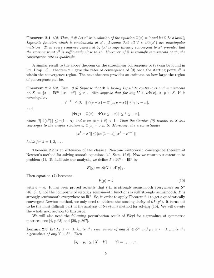
Theorem 2.1 [42, Thm. 3.2] Let x∗ be a solution of the equation Φ(x) = 0 and let Φ be a locallyLipschitz function which is semismooth at x∗. Assume that all V ∈ ∂Φ(x∗) are nonsingularmatrices. Then every sequence generated by (9) is superlinearly convergent to x∗ provided thatthe starting point x0 is sufficiently close to x∗. Moreover, if Φ is strongly semismooth at x∗, theconvergence rate is quadratic.

A similar result to the above theorem on the superlinear convergence of (9) can be found in[32, Prop. 3]. Theorem 2.1 gave the rates of convergence of (9) once the starting point x0 iswithin the convergence region. The next theorem provides an estimate on how large the regionof convergence can be.

Theorem 2.2 [42, Thm. 3.3] Suppose that Φ is locally Lipschitz continuous and semismoothon S := {x ∈ IRm | ||x − x0‖ ≤ r}. Also suppose that for any V ∈ ∂Φ(x), x, y ∈ S, V isnonsingular,

‖V −1‖ ≤ β, ‖V (y − x) − Φ′(x; y − x)‖ ≤ γ‖y − x‖,

and‖Φ(y) − Φ(x) − Φ′(x; y − x)‖ ≤ δ‖y − x‖,

where β‖Φ(x0)‖ ≤ r(1 − α) and α := β(γ + δ) < 1. Then the iterates (9) remain in S andconverges to the unique solution of Φ(x) = 0 in S. Moreover, the error estimate

‖xk − x∗‖ ≤ [α/(1 − α)]‖xk − xk−1‖

holds for k = 1, 2, . . . .

Theorem 2.2 is an extension of the classical Newton-Kantorovich convergence theorem ofNewton’s method for solving smooth equations [40, Sect. 12.6]. Now we return our attention toproblem (1). To facilitate our analysis, we define F : IRn 7→ IRn by

F (y) := A(G + A∗y)+.

Then equation (7) becomesF (y) = b (10)

with b = e. It has been proved recently that (·)+ is strongly semismooth everywhere on Sn

[46, 8]. Since the composite of strongly semismooth functions is still strongly semismooth, F isstrongly semismooth everywhere on IRn. So, in order to apply Theorem 2.1 to get a quadraticallyconvergent Newton method, we only need to address the nonsingularity of ∂F (y∗). It turns outto be the most difficult part in the analysis of Newton’s method for solving (10). We will devotethe whole next section to this issue.

We will also need the following perturbation result of Weyl for eigenvalues of symmetricmatrices, see [4, p.63] and [26, p.367].

Lemma 2.3 Let λ1 ≥ · · · ≥ λn be the eigenvalues of any X ∈ Sn and µ1 ≥ · · · ≥ µn be theeigenvalues of any Y ∈ Sn. Then

|λi − µi| ≤ ‖X − Y ‖ ∀i = 1, . . . , n.

5

3 Newton’s method

In this section, we consider the nonsmooth Newton method for equation (10):

yk+1 = yk − V −1k (F (yk) − b), Vk ∈ ∂F (yk), k = 0, 1, 2, . . . . (11)

As we briefly discussed in Section 2, the core issue for (11) is the nonsingularity of ∂F (y) wheny is near y∗, which is a solution of (10). Our main result in this section is that every element in∂F (y∗) is positive definite. Since F is already known strongly semismooth, Theorem 2.1 impliesthat method (11) is quadratically convergent if the initial point y0 is sufficiently near y∗.

To facilitate our proofs for the positive definiteness of ∂F (y∗) we need a few more notions.For any given X ∈ Sn, let λ(X) denote the eigenvalue vector of X arranged in the nonincreasingorder, i.e., λ1(X) ≥ λ2(X) ≥ · · · ≥ λn(X). Let O denote the set of all orthogonal matrices inIRn×n and OX be the set of orthonormal eigenvectors of X defined by

OX :={P ∈ O| X = PDiag[λ(X)]P T

}.

Let f : IR → IR be a continuous function. Then one can define Lowner’s function f : Sn →Sn (we adopt the convention of using f to denote both the scalar-valued and matrix-valuedfunctions) by

f(X) := PDiag[f(λ1(X)), f(λ2(X)), · · · , f(λn(X))]P T , P ∈ OX . (12)

The study on the matrix valued function f(X) defined in (12) was initiated by Lowner in hislandmark paper [33]. See Donoghue [16] and Bhatia [4] for detailed discussions on (12).

For any µ = (µ1, . . . , µn)T ∈ IRn such that f is differentiable at µ1, . . . , µn, we denote byf [1](µ) the n × n symmetric matrix whose (i, j)th entry is

(f [1](µ)

)ij

=

{f(µi) − f(µj)

µi − µjif µi 6= µj

f ′(µi) if µi = µj .

The matrix f [1](µ) is called the first divided difference of f at µ. The following result of Lowneris well known. For a proof, see Donoghue [16, Ch. VIII] or [4, Ch. V.3.3].

Lemma 3.1 Let P ∈ O be such that X = PDiag[λ1(X), · · · , λn(X)]P T . Let (a1, a2) be an openinterval in IR that contains λj(X), j = 1, . . . , n. If f is continuously differentiable on (a1, a2),then f is differentiable at X and its derivative, for any H ∈ Sn, is given by

f ′(X)H = P(f [1](λ(X)) ◦ (P T HP )

)P T . (13)

Throughout the remainder of the paper, we let f(t) = t+ := max(0, t), t ∈ IR. It is easyto derive from Moreau’s theorem on the characterization of the metric projection operator overclosed convex cones that (see [24, 50] for a proof)

X+ = f(X) = PDiag[max{λ1(X), 0},max{λ2(X), 0}, · · · ,max{λn(X), 0}]P T .

By using Lemma 3.1 (by considering any continuously differentiable scalar-valued function withvalue one on an open set containing all the nonnegative eigenvalues of X and zero on an open setcontaining all negative eigenvalues of X) and the fact that (·)+ is (continuously) differentiableat X ∈ Sn if and only if X is nonsingular, we obtain the following useful result.

6

Proposition 3.2 Let P ∈ O be such that X = PDiag[λ1(X), · · · , λn(X)]P T . Then ΠSn+(·) is

(continuously) differentiable at an X ∈ Sn with eigenvalues λ1(X), . . . , λn(X) if and only ifλi(X) 6= 0, i = 1, . . . , n. Moreover, if λi(X) 6= 0, i = 1, . . . , n, then the derivative of ΠSn

+(·) at

X, for any H ∈ Sn, is given by (13) with f(t) = t+, t ∈ IR.

See [8, Props. 4.3, 4.4] for a generalization on Proposition 3.2. We further let

C(y) := G + A∗y and λ(y) := λ(C(y)).

We define three index sets associated with λ(y):

α(y) := {i| λi(y) > 0}, β(y) := {i| λi(y) = 0} and γ(y) := {i| λi(y) < 0}.

We also let Λ(y) := Diag[λ(y)]. When no confusion is involved, we often omit y for brevity. Lety∗ be a solution of (4) throughout this section. For simplicity, we let

λ∗ := λ(y∗), α∗ := α(y∗), γ∗ := γ(y∗) and Λ∗ := Λ(y∗).

Now we present our first technical result which is a direct consequence of the positiveness of b.

Lemma 3.3 Suppose that b > 0 in (10). Then α∗ 6= ∅. Moreover, for any P ∈ OC(y∗) we have∑

`∈α∗

P 2i` > 0, ∀i = 1, . . . , n.

Proof. Suppose that P ∈ OC(y∗) is arbitrarily given. Then

(C(y∗))+ = P

Λ∗α

00

P T

and (10) implies

AP

Λ∗α

00

P T = b ,

where Λ∗α is a diagonal matrix of |α∗| × |α∗| with its diagonal elements given by λ∗

i , i ∈ α∗. Thefact that b 6= 0 implies that α∗ is not empty. Equivalently, we have

(∑

`∈α∗

λ∗`P

21`,∑

`∈α∗

λ∗`P

22`, . . . ,

∑

`∈α∗

λ∗`P

2n`

)= (b1, b2, . . . , bn).

Since λ∗` > 0 for all ` ∈ α∗, the lemma is proved to be true. �

Letδ∗ :=

12

mini∈α∗∪γ∗

|λ∗i |

andB(y∗, δ∗) := {y ∈ IRn| ‖y − y∗‖ ≤ δ∗}.

Then the perturbation result in Lemma 2.3 implies that for all y ∈ B(y∗, δ∗),

|λi(y) − λ∗i | ≤ ‖C(y) − C(y∗)‖ ≤ ‖y − y∗‖ ≤ δ∗ ∀ i = 1, . . . , n.

7

Lemma 3.4 F is differentiable at y if and only if f is differentiable at C(y). And in this case

F ′(y)h = Af ′(C(y))H ∀h ∈ IRn ,

where H := A∗h = Diag[h] and

f ′(C(y))H = P(f [1](λ(y)) ◦ (P T HP )

)P T ∀P ∈ OC(y).

Moreover, when y ∈ B(y∗, δ∗), we have(f [1](λ(y))

)ij

= 1 ∀ i, j ∈ α∗

and (f [1](λ(y))

)ij

= 0 ∀ i, j ∈ γ∗,

i,e., (f [1](λ(y))

)α∗α∗

= Eα∗α∗ ,(f [1](λ(y))

)γ∗γ∗

= 0γ∗γ∗ . (14)

Proof. It is obvious that if f is differentiable at C(y), then F is differentiable at y becauseit is composition of f with linear transformations.

Suppose f is not differentiable at C(y). Then Proposition 3.2 implies that f is not differ-entiable at λi(y) for some i ∈ {1, . . . , n}. The special structure of f(t) = max{0, t} yields thatλi(y) = 0. Since f(t) is directionally differentiable and nondecreasing, it holds that

f ′(x; 1) ≥ f ′(x;−1) ∀x ∈ IR.

In particular,f ′(λi; 1) = 1 > 0 = f ′(λi;−1).

We let d, d ∈ IRn be defined respectively by

d` = f ′(λ`; 1) and d` = f ′(λ`;−1), ` = 1, . . . , n.

Since di = 1 > di = 0, we see that d 6= d and d ≥ d. Consider two sequences respectivelyspecified by {y + te}t>0 and {y − te}t>0. We have

C(y + te) = PDiag[λ + te]P T and C(y − te) = PDiag[λ − te]P T , P ∈ OC(y).

Hence,

limt↓0

F (y + te) − F (y)t

= APDiag[d]P T and limt↓0

F (y − te) − F (y)−t

= APDiag[d]P T .

With a bit further calculation, we see by noticing d` ≥ d` for ` = 1, . . . , n and di > di that

APDiag[d]P T −APDiag[d]P T =

∑n`=1(d` − d`)P 2

1`...∑n

`=1(d` − d`)P 2n`

6= 0.

8

This means thatlimt↓0

F (y + te) − F (y)t

6= limt↓0

F (y − te) − F (y)−t

,

implying that F is not differentiable at y. This establishes the first part of the lemma.The formula for F ′ just follows from the chain rule and Proposition 3.2. The relation in (14)

follows from the definition of f [1] and the fact that for any y ∈ B(y∗, δ∗), λi(y) > 0 for all i ∈ α∗

and λi(y) < 0 for all i ∈ γ∗. �

We now define a collection of matrices in relation to λ∗:

M :=

M ∈ IRn×n | M =

Eα∗α∗ Eα∗β∗ (τij) i∈α∗j∈γ∗

Eβ∗α∗ (ωij) i∈β∗j∈β∗

0

(τji) i∈α∗j∈γ∗

0 0

,

ωij = ωji ∈ [0, 1]for i, j ∈ β∗

τij = λ∗i /(λ

∗i − λ∗

j)for i ∈ α∗, j ∈ γ∗

.

We note that M is a compact set and 1 > τij > 0 for any M ∈ M.

Lemma 3.5 For any h ∈ IRn we have

∂BF (y∗)h ⊆ {AWH : W ∈ W} ,

where H := A∗h = Diag[h] and

W :={W | WH = P

(M ◦ (P T HP )

)P T , P ∈ OC(y∗), M ∈ M and h ∈ IRn

}.

Proof. Let V ∈ ∂BF (y∗). By the very definition of ∂BF we have a sequence {yk} convergingto y∗ such that F is differentiable at each yk and F ′(yk) → V . Equivalently, we have

limk→∞

F ′(yk)h = V h ∀h ∈ IRn. (15)

Then it follows from Lemma 3.4 that there exists P k ∈ OC(yk) such that

F ′(yk)h = Af ′(C(yk))H,

where H = A∗h = Diag[h] and

f ′(C(yk))H = P k(f [1](λ(yk)) ◦ ((P k)T HP k)

)(P k)T .

Denoting λk := λ(yk) for simplicity. When yk ∈ B(y∗, δ∗),

λki > 0 for i ∈ α∗ and λk

i < 0 for i ∈ γ∗,

and λki for i ∈ β∗ could be positive or nonpositive, but converges to λ∗

i = 0. Hence, the definitionof f [1] yields

(f [1](λk)

)ij

=

1, i, j ∈ α∗

0, i, j,∈ γ∗

λki − (λk

j )+λk

i − λkj

, i ∈ α∗, j ∈ β∗

λki

λki − λk

j

, i ∈ α∗, j ∈ γ∗

9

and (f [1](λk))ij = (f [1](λk))ji (i.e., it is symmetric). Because 0 ≤ (f [1](λk))ij ≤ 1 for all i, j,there exists a sequence (still denoted by {yk} without loss of generality) such that f [1](λk)converges to a matrix, say M∗. It is easy to see that M∗ ∈ M. The boundedness of {P k} alsoimplies that there exists a sequence (also denoted by {yk}) such that P k → P ∗. Then we have

C(y∗) = limk→∞

C(yk) = limk→∞

P kDiag[λk](P k)T = P ∗Diag[λ](P ∗)T .

Hence, P ∗ ∈ OC(y∗) and consequently we have by (15) that

V h = limk→∞

F ′(yk)h ∈ {AWH : W ∈ W} ∀h ∈ IRn.

Since V ∈ ∂BF (y∗) is arbitrary, we establish our result. �Now we are ready to prove our main result in this section.

Proposition 3.6 Each element V ∈ ∂BF (y∗) is positive definite. Consequently, each elementV ∈ ∂F (y∗) is also positive definite.

Proof. Let V ∈ ∂BF (y∗) be arbitrarily chosen. We want to show that for any 0 6= h ∈ IRn

hT V h > 0.

We note that it follows from Lemma 3.5 that there exist M ∈ M and P ∈ OC(y∗) such that

V h = A(P (M ◦ (P T HP )

)P T .

Then

〈h, V h〉 = 〈A∗h, P (M ◦ (P T HP ))P T 〉= 〈P T HP,M ◦ (P T HP )〉.

Let H := P T HP . Then we have

〈h, V h〉 = 〈H,M ◦ H〉

≥∑

i∈α∗

∑

j∈α∗∪β∗

H2ij +

∑

j∈γ∗

τijH2ij

≥ τ∑

i∈α∗

n∑

j=1

H2ij,

where τ = mini∈α∗,j∈γ∗ τij > 0. Because V is positive semidefinite, we see that 〈h, V h〉 = 0 onlyif

Hij = 0 ∀i ∈ α∗ and j ∈ {1, . . . , n}.

The above condition is equivalent

(Hi1, Hi2, . . . , Hin) = (0, 0, . . . , 0) ∀i ∈ α∗.

10

By recalling that H = P T HP and H = Diag[h], we have

(Hi1, Hi2, . . . , Hin) = (h1P1i, h2P2i, . . . , hnPni)P = (0, 0, . . . , 0)

if and only if

(h1P21i, h2P

22i, . . . , hnP 2

ni) = (0, 0, . . . , 0) (because P is nonsingular).

Summarizing over i ∈ α∗ in the above relation yields

(h1

∑

i∈α∗

P 21i, h2

∑

i∈α∗

P 22i, . . . , hn

∑

i∈α∗

P 2ni) = (0, 0, . . . , 0).

According to Lemma 3.3, the above condition holds if and only if

(h1, h2, . . . , hn) = (0, 0, . . . , 0),

i.e., h = 0. This establishes the positive definiteness of V .Since ∂BF (y∗) is compact and its every element is positive definite, any convex combination

of its elements is also positive definite. That is, every element of ∂F (y∗) is positive definite. �

The first of two important consequences of the above regularity result is on the convergenceof Newton’s method (11). It is just a direct application of Theorem 2.1, given that we havealready known that F is strongly semismooth and every element in ∂F (y∗) is positive definite.

Corollary 3.7 Newton’s method (11) is quadratically convergent provided that y0 is sufficientlyclose to y∗.

The second corollary is on the uniqueness of the solution to (10) and its strong semismooth-ness.

Corollary 3.8 For any given G ∈ Sn and 0 < b ∈ IRn, there is a unique solution y∗ to equation(10). If y∗ is viewed as a function of G and b, denoted y∗(G, b), then y∗ is strongly semismoothwith respect to (G, b) ∈ Sn × IRn

++. Consequently, X∗ as a function of G and b is also stronglysemismooth with respect to (G, b) ∈ Sn × IRn

++.

Proof. The proof for Prop. 3.6 is independent of the choice of G and b as long as it belongsto Sn × IRn

++. Hence, the Clarke inverse theorem says that there is a unique solution y∗(G, b)for any (G, b) ∈ Sn × IRn

++. We note that the existence of a solution is guaranteed because0 < b ∈ IRn

++ and b ∈ intA(Sn+). The strong semismoothness of y∗ follows from a result of

Sun [45] on an implicit theorem of strongly semismooth functions. Since X∗ is a composition ofstrongly semismooth functions, it is also strongly semismooth with respect to (G, b) ∈ Sn×IRn

++.�

11

4 Extensions

4.1 The W -weighted version

In practice, the W -weighted version of (1) is very useful [25]:

min12‖G − X‖2

W

s.t. Xii = 1, i = 1, . . . , nX � 0,

(16)

where W ∈ Sn is positive definite and for any Y ∈ Sn,

‖Y ‖W = ‖W 1/2Y W 1/2‖.

LetG = W 1/2GW 1/2 and X = W 1/2XW 1/2 .

Then problem (16) becomes standard in the form of (1):

min12‖G − X‖2

s.t.(W−1/2XW−1/2

)ii

= 1, i = 1, . . . , nX � 0.

In fact, the constraint X � 0 should be W−1/2XW−1/2 � 0. It is easy to see that they areequivalent. For simplicity, we drop the bars in the above formulation and have

min12‖G − X‖2

s.t.(W−1/2XW−1/2

)ii

= 1, i = 1, . . . , nX � 0.

(17)

Define the linear operator A : Sn 7→ IRn by

(AX)i =(W−1/2XW−1/2

)ii

, i = 1, . . . , n. (18)

The adjoint operator A∗ : IRn 7→ Sn is given by

〈A∗y,X〉 = 〈y,AX〉= 〈y,diag[W−1/2XW−1/2]〉= 〈Diag[y],W−1/2XW−1/2〉= 〈W−1/2Diag[y]W−1/2,X〉.

HenceA∗y = W−1/2Diag[y]W−1/2. (19)

It is easy to see that e ∈ intASn+. With this fact, we once again get equation (10) with A and

A∗ defined by (18) and (19) respectively. With no difficulty, we can develop parallel results asin Lemmas 3.3–3.5 and in Proposition 3.6. For example, Lemma 3.3 now becomes

12

Lemma 4.1 Suppose that b > 0 in (10) and that A and A∗ are defined by (18) and (19)respectively. Then α∗ 6= ∅. Moreover, for any P ∈ OC(y∗) we have

∑

`∈α∗

P 2i` > 0, ∀i = 1, . . . , n ,

where P = W−1/2P .

The proof just follows that of Lemma 3.3 and makes use of (18). Lemmas 3.4 and 3.5 remaintrue with H = A∗h = W−1/2Diag[h]W−1/2 for h ∈ IRn. The proof for Proposition 3.6 is alsotrue with now H = P T HP and H is as just defined. Starting from

(Hi1, Hi2, . . . , Hin) = (0, 0, . . . , 0) ∀i ∈ α∗

in the proof of Proposition 3.6, we have

(h1

∑

i∈α∗

P 21i, h2

∑

i∈α∗

P 22i, . . . , hn

∑

i∈α∗

P 2ni) = (0, 0, . . . , 0)

by noticingH = P T W−1/2Diag[h]W−1/2P = PDiag[h]P .

According to Lemma 4.1, the above condition holds if and only if

(h1, h2, . . . , hn) = (0, 0, . . . , 0).

This proves Proposition 3.6 with A and A∗ defined by (18) and (19) respectively. Therefore, forthe W -weighted version, Newton’s method is quadratically convergent.

4.2 The case of lower bounds

The nearest correlation matrix is often rank-deficient [25]. To avoid the ill-conditionedness andto increase the stability, one often requires the matrix to be not less than a positive diagonalmatrix. This gives the so-called the calibration of correlation matrices, i.e.,

min 12‖G − X‖2

s.t. X � αIAX = e ,

(20)

where α ∈ (0, 1) and AX = diag[X]. We will see that it is quite straightforward to apply thegeneralized Newton method to this case.

First we note that the following condition is automatically valid:{A∗y : (1 − α)yT e ≥ 0, y ∈ IRn

}∩ (−Sn

+) = {0}.

This condition corresponds to the condition [37, (2.17)], so that [37, Thm. 2.2] (This theoremonly considers the case which corresponds to G = 0 in (20); however, it also holds for G 6= 0)implies that the unique solution of (20) has the following representation:

X∗ = (G − αI + A∗y∗)+ + αI,

13

where y∗ is a solution of the following equation:

A(G − αI + A∗y)+ + αAI = e,

which is obviously equivalent to

A(G − αI + A∗y)+ = (1 − α)e. (21)

We now note that this equation actually defines a new problem similar to (1):

min 12‖(G − αI) − X‖2

s.t. Ae = (1 − α)eX ∈ Sn

+.

(22)

Hence, by following the discussion in Section 1 and noting that (1 − α)e > 0, we know that theunique solution of problem (22) has the form

X∗ = (G − αI + A∗y∗)+,

where y∗ is the unique solution of (21). We note that the uniqueness of y∗ follows from Corol-lary 3.8 applied to (22). Therefore, Newton’s method also applies to (21) and is quadraticallyconvergent by Corollary 3.7, and hence solves (20).

A more complicated problem of the calibration of covariance matrix was also discussed byMalick [35] and is defined by

min 12‖X − Q‖2

s.t. X � αI

〈I,X〉 = tr(Q)〈Gi,X〉 = σ2

i , i = 1, . . . ,m

(23)

where α > 0, Q is a first estimate of the true covariance matrix Q used in portfolio risk analysis,and σ2

i represent “ex-post” volatilities of well-chosen portfolios; Gi ∈ Sn. We now demonstratehow Newton’s method can be applied to this problem.

The feasibility of problem (23) requires

tr(Q) ≥ nα.

To facilitate our analysis, let

b0 := tr(Q), bi := σ2i , i = 1, . . . ,m and b := (b0, b1, . . . , bm)T ∈ IRm+1,

G0 := I, A := (G0, G1, . . . , Gm)

withAX := (〈G0,X〉, 〈G1,X〉, . . . , 〈Gm,X〉)T ∈ IRm+1.

Suppose that Gi’s are positive semidefinite nonzero matrices. Then tr(Gi) > 0 for each i. Let αbe chosen such that

0 < α < min{bi/tr(Gi) | i = 0, 1, . . . ,m}. (24)

14

We also assume that if for any y ∈ IRm+1 with y` > 0 for some ` ∈ {0, 1, . . . ,m}, we have

A∗y :=m∑

i=1

Giyi 6� 0. (25)

Conditions (24) and (25) indicate how α and Gi are chosen in problem (23). Under these twoconditions, we see that condition (2.17) in [37] is valid for problem (23), i.e.,

{A∗y : yT (b − αz0) ≥ 0} ∩ (−Sn+) = {0},

where z0 := AI = (tr(G0), tr(G1), . . . , tr(Gm))T ∈ IRm+1. Hence, once again [37, Thm. 2.2]implies that the unique solution of (23) has the representation:

X∗ = (Q − αI + A∗y∗)+ + αI ,

where y∗ is a solution to the following equation:

A(Q − αI + A∗y)+ = b − αz0. (26)

Now the generalized Newton method can be applied to this equation. If we further assume thatthe matrices Gi, i = 1, . . . ,m are mutually diagonalizable, Newton’s method is also quadraticallyconvergent following our results in the last section. To see this, let P ∈ O be a matrix such thatGi are simultaneously diagonalizable by P , i.e.,

Gi = PΓiP T , i = 1, . . . ,m,

where each Γi is a nonnegative diagonal matrix. Let Γ0 = I and define

L := (Γ0,Γ1, . . . ,Γm)

so thatLX = (〈Γ0,X〉, 〈Γ1,X〉, . . . , 〈Γm,X〉)T

and

L∗y =m∑

i=0

Γiyi.

Then equation (26) becomes

L(P T (Q − αI)P + L∗y)+ = b , (27)

where b := diag[P T (b−αz0)P ]. Since b−αz0 > 0 by the assumed conditions, we see that b > 0.Now we note that equation (27) defines a new problem given by

min 12‖P

T (Q − αI)P − X‖2

s.t. 〈Γi,X〉 = bi, i = 0, . . . ,mX ∈ Sn

+.

It is easy to repeat the arguments for problem (1) to verify that Newton’s method for the aboveproblem is quadratically convergent.

Finally we note that all the assumptions made so far for problem (23) are automaticallysatisfied if each Gi = Ei, where Ei is the diagonal matrix whose only nonzero element is its ithdiagonal element and equals 1.

15

4.3 The nonsymmetric case

In some applications [31], X may be only required to be positive semidefinite but not necessarilysymmetric. Then we have the following matrix nearness problem

min12‖X − G ‖2

s.t. AX = bX ∈ Kn ,

(28)

where Kn is the cone of n × n positive semidefinite matrices (not necessarily symmetric)

Kn = {X ∈ IRn×n |X is positive semidefinite} .

By assuming the strong CHIP on {Kn,A−1(b)}, we know from Section 1 that the unique solutionX∗ to problem (28) has the representation

X∗ = ΠKn(G + A∗y∗) (29)

and y∗ is a solution of the equation

F (y) := AΠKn(G + A∗y) = b, y ∈ IRn . (30)

Next, we derive an explicit formula for computing ΠKn(X) for a given X ∈ IRn×n. It is easyto see that ΠKn(X) is the unique solution to

min12‖Y − X ‖2

s.t.12(Y + Y T ) ∈ Sn

+ .(31)

Since the Slater condition for problem (31) holds automatically, ΠKn(X), together with theLagrange multiplier Λ ∈ Sn

+, satisfies the KKT conditions [34, Ch.8]{

Y − X − Λ = 0,12(Y + Y T ) ∈ Sn

+ , Λ ∈ Sn+ ,

12(Y + Y T )Λ = 0 .

These conditions can be equivalently written as{

Y − X − Λ = 0,Λ − ΠSn

+[Λ − 1

2 (Y + Y T )] = 0 ,

which imply

Λ − 12(Y + Y T ) = −1

2(X + XT )

andΛ =

12ΠSn

+[−(X + XT )] .

HenceΠKn(X) = X +

12ΠSn

+[−(X + XT )] =

12(X − XT ) +

12ΠSn

+(X + XT ) .

Therefore, by [46, Thm 4.13], we get

16

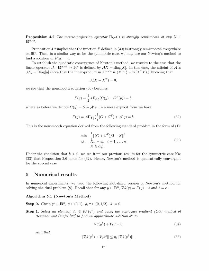
Proposition 4.2 The metric projection operator ΠKn(·) is strongly semismooth at any X ∈IRn×n.

Proposition 4.2 implies that the function F defined in (30) is strongly semismooth everywhereon IRn. Then, in a similar way as for the symmetric case, we may use our Newton’s method tofind a solution of F (y) = b.

To establish the quadratic convergence of Newton’s method, we restrict to the case that thelinear operator A : IRn×n 7→ IRn is defined by AX = diag[X]. In this case, the adjoint of A isA∗y = Diag[y] (note that the inner-product in IRn×n is 〈X,Y 〉 = tr(XT Y ).) Noticing that

A(X − XT ) = 0,

we see that the nonsmooth equation (30) becomes

F (y) =12AΠSn

+(C(y) + CT (y)) = b,

where as before we denote C(y) = G + A∗y. In a more explicit form we have

F (y) = AΠSn+(12(G + GT ) + A∗y) = b. (32)

This is the nonsmooth equation derived from the following standard problem in the form of (1):

min12‖(G + GT )/2 − X‖2

s.t. Xii = bi, i = 1, . . . , nX ∈ Sn

+ .

(33)

Under the condition that b > 0, we see from our previous results for the symmetric case like(33) that Proposition 3.6 holds for (32). Hence, Newton’s method is quadratically convergentfor the special case.

5 Numerical results

In numerical experiments, we used the following globalized version of Newton’s method forsolving the dual problem (8). Recall that for any y ∈ IRn, ∇θ(y) = F (y) − b and b = e.

Algorithm 5.1 (Newton’s Method)

Step 0. Given y0 ∈ IRn, η ∈ (0, 1), ρ, σ ∈ (0, 1/2). k := 0.

Step 1. Select an element Vk ∈ ∂F (yk) and apply the conjugate gradient (CG) method ofHestenes and Stiefel [23] to find an approximate solution dk to

∇θ(yk) + Vkd = 0 (34)

such that‖∇θ(yk) + Vkd

k‖ ≤ ηk‖∇θ(yk)‖ , (35)

17

where ηk := min{η, ‖∇θ(yk)‖}. If (35) is not achievable or if the condition

∇θ(yk)T dk ≤ −ηk‖dk‖2 (36)

is not satisfied, let dk := −B−1k ∇θ(yk), where Bk is any symmetric positive definite matrix

in Sn.

Step 2. Let mk be the smallest nonnegative integer m such that

θ(yk + ρmdk) − θ(yk) ≤ σρm∇θ(yk)T dk.

Set tk := ρmk and yk+1 := yk + tkdk.

Step 3. Replace k by k + 1 and go to Step 1.

An alternative to calculating the Newton direction is to apply the CG method to the followingperturbed Newton equation:

∇θ(yk) + (Vk + εkI) d = 0 with εk > 0.

The classical choice of εk is the norm of the residue, i.e., εk = ‖F (yk) − b‖. Since Vk is alwayspositive semidefinite, the matrix (Vk + εkI) is always positive definite for any εk > 0.

The global convergence analysis of Algorithm 5.1 is quite standard. Since the CG methodis used to calculate the Newton direction, it is actually an inexact Newton direction that wasused in our implementation. Hence, our local convergence analysis is a bit different from thestandard ones. We provide a proof for the sake of completeness.

First, we need the following result due to Facchinei [21, Thm. 3.3 & Remark 3.4]. A similarresult was also obtained by Pang and Qi [41].

Lemma 5.2 Suppose that, for every k,

∇θ(yk)T dk ≤ −ρ‖dk‖2

for some ρ > 0. Then, for any µ ∈ (0, 1/2), there exists a k such that for all k ≥ k,

θ(yk + dk) ≤ θ(yk) + µ∇θ(yk)T dk .

Theorem 5.3 Suppose that in Algorithm 5.1 both {‖Bk‖} and {‖B−1k ‖} are uniformly bounded.

Then the iteration sequence {yk} generated by Algorithm 5.1 converges to the unique solution y∗

of F (y) = b quadratically.

Proof. Since for any k ≥ 0, dk is always a descent direction of θ(·) at yk, Algorithm 5.1 iswell defined. Moreover, from the coercive property of θ we know that {yk} is bounded. Then,by employing standard convergence analysis (cf. [12, Thm 6.3.3]), we can conclude that

limk→∞

∇θ(yk) = 0 ,

which, together with the convexity of θ(·) and the boundedness of {yk}, implies that yk → y∗.

18

Since, by Proposition 3.6, any element V ∈ ∂F (y∗) is positive definite, it holds that for allk sufficiently large, Vk is positive definite and {‖V −1

k ‖} is uniformly bounded. Hence, for all ksufficiently large, the CG method can find dk such that both (35) and (36) are satisfied. This,together with the facts that ∇θ(y∗) = 0 and ∇θ(·) is strongly semismooth at y∗, further impliesthat for all k sufficiently large,

‖yk + dk − y∗‖ = ‖yk + V −1k [(∇θ(yk) + Vkd

k) −∇θ(yk)] − y∗‖

≤ ‖yk − y∗ − V −1k ∇θ(yk)‖ + ‖V −1

k (∇θ(yk) + Vkdk)‖

≤ ‖V −1k ‖‖∇θ(yk) −∇θ(y∗) − Vk(yk − y∗)‖ + ηk‖V −1

k ‖‖∇θ(yk)‖

≤ O(‖yk − y∗‖2) + ‖V −1k ‖‖∇θ(yk)‖2

≤ O(‖yk − y∗‖2) + O(‖∇θ(yk) −∇θ(y∗)‖)2,

= O(‖yk − y∗‖2), (37)

where in the last equality we used the Lipschitz continuity of ∇θ(·). From (37) and the factthat yk → y∗, we have for all k sufficiently large that

yk − y∗ = −dk + O(‖dk‖2) and ‖dk‖ → 0. (38)

For each k ≥ 0, let rk := ∇θ(yk) + Vkdk. Then for all k sufficiently large,

−∇θ(yk)T dk = 〈dk, Vkdk〉 − 〈dk, rk〉

≥ 〈dk, Vkdk〉 − ‖dk‖‖rk‖

≥ 〈dk, Vkdk〉 − ηk‖dk‖‖∇θ(yk)‖

= 〈dk, Vkdk〉 − ‖dk‖‖∇θ(yk)‖2

≥ 〈dk, Vkdk〉 − ‖dk‖‖yk − y∗‖2, (39)

which, together with (38) and the uniform positive definiteness of Vk, implies that there existsρ > 0 such that for all k sufficiently large,

−∇θ(yk)T dk ≥ ρ‖dk‖2.

It then follows from Lemma 5.2 that for all k sufficiently large tk = 1 and

yk+1 = yk + dk .

The proof is completed by observing (37). �

Next, we discuss several issues regarding the implementation of Algorithm 5.1.

(a) Forming the Newton matrix. In Algorithm 5.1, we need to find a V ∈ ∂F (y) to formequation (34). For a given y ∈ IRn, let C(y) have the following spectral decomposition

C(y) = PDiag[λ(y)]P T , P ∈ OC(y).

19

Let

My :=

Eαα Eαβ (τij(y)) i∈αj∈γ

Eβα 0 0(τji(y)) i∈α

j∈γ0 0

, τij(y) :=

λi(y)λi(y) − λj(y)

, i ∈ α, j ∈ γ.

Define the matrix Vy ∈ IRn×n by

Vyh = AP(My ◦ (P T HP )

)P T , h ∈ IRn , (40)

where H := Diag[h].

Proposition 5.4 Let the matrix Vy be defined by (40). Then

Vy ∈ ∂BF (y) ⊆ ∂F (y).

Proof. Recall that the scalar-valued function f(t) = max(0, t), t ∈ IR. For each k > 0, lettk := −1/k. We now consider the sequence {zk} with zk given by zk := y − tke = y + (1/k)e.Then, λ(y) − tke is the spectrum of C(zk), i.e.,

C(zk) = C(y) − tkC(e) = PDiag[λ(y) − tke]P T = PDiag[λ(y) + (1/k)e]P T .

Let k > 0 be sufficiently large such that 1/k < min{|λi(y)| | i ∈ α ∪ γ} (recall the definitions ofα and γ). Then, for each k ≥ k, the matrix valued function f : Sn → Sn is differentiable atC(zk) because C(zk) is nonsingular and in this case, by Lemma 3.1, f is differentiable at C(zk)and for any Z ∈ Sn,

f ′(C(zk))Z = P(f [1](λ(y) + (1/k)e) ◦ (P T ZP )

)P .

Therefore, from Lemma 3.4 we know that for each k ≥ k, F is differentiable at zk and for anyh ∈ IRn,

F ′(zk)h = Af ′(C(zk))H,

where H := Diag[h]. After direct computations we can see that

My = limk→∞

f [1](λ(y) + (1/k)e).

Hence, for each h ∈ IRn,

limk→∞

F ′(zk)h = AP(My ◦ (P T HP )

)P T ,

which, together with (40), implies that

Vy = limk→∞

F ′(zk).

20

Thus, by the definition of ∂BF (y), Vy ∈ ∂BF (y). The proof is completed by observing that∂F (y) = co ∂BF (y). �

We see from Proposition 5.4 that we can obtain an element Vy ∈ ∂F (y) by the spectraldecomposition of C(y). Since we use the CG method to solve (34), we do not need to form Vy

explicitly.(b) Testing examples. We tested the following four classes of problems:

Example 5.5 C is a randomly generated n×n correlation matrix by MATLAB 7.0.1’s gallery(’randcorr’,n). R is a random n × n symmetric matrix with Rij ∈ [−1, 1], i, j = 1, 2, . . . , n.Then we set

G = C + αR ,

where α = 0.01, 0.1, 1.0, 10.0. We fix n = 1000 in our numerical reports. This problem wastested by Higham [25].

Example 5.6 G is a randomly generated symmetric matrix as in the first example of Malick[35] with Gij ∈ [−1, 1] and Gii = 1.0, i, j = 1, 2, . . . , n and n = 500, 1000, 1500, 2000.

Example 5.7 G is a randomly generated symmetric matrix with Gij ∈ [0, 2] and Gii = 1.0,i, j = 1, 2, . . . , n and n = 500, 1000, 1500, 2000.

Example 5.8 G is a randomly generated symmetric matrix as in the second example of Malick[35] with

Gii ∈ [−2.0 × 104, 2.0 × 104], i = 1, 2, . . . , n.

We add to G a perturbed n × n random symmetric matrix with entries in [−α, α], where α =0.0, 0.01, 0.1, 1.0. We report our numerical results for n = 1000.

(c) Initial parameters. In our numerical experiments, two initial points were used: (i) b −diag(G); and (ii) b − diag(G) + e. Other initial points may be used. For example, we maystart from a positive point, i.e., y0 > 0, such that C(y0) is positive definite. The performanceof Newton’s method is similar as we reported below. We set other parameters as η = 10−5,ρ = 0.5, and σ = 2.0 × 10−4. For simplicity, we fix Bk ≡ I for all k ≥ 0.

(d) Comparison and observations. For the purpose of comparison, we tested the performanceof the BFGS method with the Wolfe line-search used by Malick [35] and the alternating projec-tion method employed by Higham [25]. The details of the implementation of the BFGS methodcan be found in [39, Ch. 8]. As observed by Malick [35, Thm. 5.1], Higham’s method is thefollowing standard gradient optimization algorithm applied to (8):

yk+1 := yk −∇θ(yk) , k = 0, 1, . . . ,

and is therefore called the gradient method. We also tested a hybrid method that combines theBFGS method and Newton’s method. The hybrid method, which is called BFGS-N here, startswith the BFGS method and switches to Newton’s method when ‖∇θ(yk)‖ ≤ 1.0.

21

All tests were carried out in MATLAB 7.0.1 running on a PC Pentium IV. In our experiments,our stopping criterion is

‖∇θ(yk)‖ ≤ 10−5 .

The reason that we chose 10−5 instead of 10−6 or higher accuracy is because the the BFGSmethod and the gradient method ran into difficulty for a higher accuracy in a few cases. Ournumerical results are reported in Tables 1-4, where Init., Iter., Func., and Res. stand for, respec-tively, the initial point used, the number of iterations and the number of function evaluationsof θ, and the residual ‖∇θ(yk)‖ at the final iterate of an algorithm (we set a maximum of 500iterations). LS failed means that the line search failed (the steplength is too small to proceed)during the computation.

An outstanding observation is that Newton’s method took less than 10 iterations for allthe problems to reach the reported accuracy and the quadratic convergence was observed. TheBFGS method performed quite well for Examples 5.5, 5.6, and 5.8 while there are four linesearch failures in Example 5.7. Sometimes it took much longer time to reach the requiredaccuracy. Numerical results for BFGS-N clearly showed that Newton’s method can be used tosave a lot of computing time required by the BFGS method. The gradient method is generallyoutperformed by the BFGS method. Compared with the numerical results reported in [49]on the inexact primal-dual path following interior point methods (IMPs) for the similar testedexamples, our proposed Newton method is much faster (4 to 5 times) in terms of the cputime.The main reason is that the proposed Newton method needs fewer number of iterations andat each iteration it needs only one eigenvalue decomposition instead of two as in the inexactprimal-dual path following IMPs [49].

More specific observations are included in the following remarks.

Remark 5.9 Newton’s method takes less cputime and less number of iterations. For all thetested examples, it is observed that the Newton method always took the unit steplength andachieved the quadratic convergence at the last several iterations. Typically, Newton’s methodwas terminated in two or three steps after the residue of the gradient is below 10−1 or 10−2.

Remark 5.10 The major cost in Newton’s method includes two parts: 1) the spectral decompo-sition; and 2) the CG method for solving the linear system. In order to form the linear system,we need the computation of the full eigensystem. So it seems that the computing time involvedin part 1) is inevitable. The computing time in part 2) may be reduced by making use of thespecial structure of ∂BF (y), y ∈ IRn. We did not explore the latter in our implementation as weare quite satisfied with the performance of Newton’s method.

Remark 5.11 The major cost in the BFGS method and the gradient is the spectral decomposi-tion. By doing a partial spectral decomposition as outlined in [25], we may be able to save somecputime. We did not exploit this as we do not know the distributions of the eigenvalues of theoptimal correlation matrix.

Remark 5.12 It can be seen clearly from the numerical results for BFGS-N that Newton’ssteps reduced the cputime committed by the BFGS method substantially. If one can calculateF (y) much less costly than via the computation of the full eigensystem, then it may be a good

22

choice to start with a method like the BFGS, which costs less than Newton’s method at each step,and then switch to Newton’s method when the iterates are close to the solution. In this case,BFGS-N may be an ideal choice.

6 Conclusion

In this paper, a close look at the nearest correlation matrix problem as the best approximationfrom a convex set in a Hilbert space lead us to consider Newton’s method. Theoretically, weproved that Newton’s method is well defined and is quadratically convergent. Our theoreticalresults were then extended to such problems as the W -weighted nearest correlation problem, thecase with lower bounds and the nonsymmetric case. Numerically, Newton’s method is shownto be extremely efficient, taking less than 10 iterations to solve all the test problems. Thisresearch opens the possibility of developing Newton’s method for other least-square semidefiniteproblems. We shall pursue this possibility in our future research.

Acknowledgement. The authors are grateful to Professor N.J. Higham for suggesting thepresent title and the referees for their helpful comments.

References

[1] L.-E. Andersson and T. Elfving, An algorithm for constrained interpolation, SIAMJ. Sci. Statist. Comput. 8 (1987), pp. 1012–1025.

[2] H.H. Bauschke, J.M. Borwein, and W. Li, Strong conical hull intersection property,bounded linear regularity, Jameson’s property (G), and error bounds in convex optimiza-tion, Math. Program. 86 (1999), pp. 135–160.

[3] H.H. Bauschke, J.M. Borwein, and P. Tseng, Bounded linear regularity, strongCHIP, and CHIP are distinct properties, J. Convex Anal. 7 (2000), pp. 395–412.

[4] R. Bhatia, Matrix Analysis, Springer-Verlag, New York, 1997.

[5] J. Borwein and A. S. Lewis, Partially finite convex programming I: Quasi relativeinteriors and duality theory, Math. Programming 57 (1992), pp. 15–48.

[6] J. Borwein and H. Wolkowicz, A simple constraint qualification in infinite-dimensional programming, Math. Programming 35 (1986), pp. 83–96.

[7] S. Boyd and L. Xiao, Least-squares covariance matrix adjustment, Technical report,Department of Electrical Engineering, Stanford University, June 2004.

[8] X. Chen, H.-D. Qi, and P. Tseng, Analysis of nonsmooth symmetric matrix valuedfunctions with applications to semidefinite complementarity problems, SIAM J. Optim. 13(2003), pp. 960–985.

23

[9] C.K. Chui, F. Deutsch, and J.D. Ward, Constrained best approximation in Hilbertspace, Constr. Approx. 6 (1990), pp. 35–64.

[10] C.K. Chui, F. Deutsch, and J.D. Ward, Constrained best approximation in Hilbertspace II, J. Approx. Theory 71 (1992), pp. 213–238.

[11] F.H. Clarke, Optimization and Nonsmooth Analysis, John Wiley & Sons, New York,1983.

[12] J.E. Dennis and R.B. Schnabel, Numerical Methods for Unconstrained Optimizationand Nonlinear Equations, Prentice-Hall, New Jersey, 1983.

[13] F. Deutsch, Best Approximation in Inner Product Spaces, CMS Books in Mathematics7, Springer-Verlag, New York, 2001.

[14] F. Deutsch, W. Li, and J.D. Ward, A dual approach to constrained interpolation froma convex subset of Hilbert space, J. Approx. Theory 90 (1997), pp. 385–414.

[15] F. Deutsch, W. Li, and J.D. Ward, Best approximation from the intersection of aclosed convex set and a polyhedron in Hilbert space, weak Slater conditions, and the strongconical hull intersection property, SIAM J. Optim. 10 (1999), pp. 252–268

[16] W.F. Donoghue, Monotone Matrix Functions and Analytic Continuation, Springer, NewYork, 1974.

[17] A. L. Dontchev and B. D. Kalchev, Duality and well-posedness in convex interpola-tion, Numer. Funct. Anal. and Optim. 10 (1989), pp. 673-689.

[18] A. L. Dontchev, H.-D. Qi, and L. Qi, Convergence of Newton’s method for convexbest interpolation, Numer. Math. 87 (2001), pp. 435–456.

[19] A. L. Dontchev, H.-D. Qi, and L. Qi, Quadratic convergence of Newton’s method forconvex interpolation and smoothing, Constr. Approx. 19 (2003), pp. 123–143.

[20] R.L. Dykstra, An algorithm for restricted least squares regression, J. Amer. Stat. Assoc.78 (1983), pp. 837–842.

[21] F. Facchinei, Minimization of SC1 functions and the Maratos effect, Oper. Res. Lett.17 (1995), pp. 131–137.

[22] J. Favard, Sur l’interpolation, J. Math. Pures Appl. 19 (1940), pp. 281–306.

[23] M.R. Hestenes and E. Stiefel, Methods of conjugate gradients for solving linear sys-tems, J. Res. Nat. Bur. Stand. 49 (1952), pp. 409–436.

[24] N.J. Higham, Computing a nearest symmetric positive semidefinite matrix, Linear Alge-bra Appl. 103 (1988), pp. 103–118. 1988.

[25] N.J. Higham, Computing the nearest correlation matrix – a problem from finance, IMAJ. Numer. Analysis 22 (2002), pp. 329–343.

24

[26] R.A. Horn and C.R. Johnson, Matrix Analysis, Cambridge University Press, Cam-bridge, UK, 1985.

[27] U. Hornung, Interpolation by smooth functions under restriction on the derivatives, J.Approx. Theory 28 (1980), pp. 227–237.

[28] L. D. Irvine, S. P. Marin, and P. W. Smith, Constrained interpolation and smoothing,Constr. Approx. 2 (1986), pp. 129–151.

[29] G. Iliev and W. Pollul, Convex interpolation by functions with minimal Lp norm(1 < p < ∞) of the kth derivative, Mathematics and mathematical education (SunnyBeach, 1984), pp. 31–42, Bulg. Akad. Nauk, Sofia, 1984.

[30] M. Kojima and S. Shindo, Extensions of Newton and quasi-Newton methods to systemsof PC1 equations, Journal of Operations Research Society of Japan 29 (1986), pp. 352-374.

[31] N. Krislock, J. Lang, J. Varah, and D. K. Pai, Local compliance estimation viapositive semidefinite constrained least squares, IEEE Transactions on Robotics and Au-tomation 20 (2004), pp. 1007–1011.

[32] B. Kummer, Newton’s method for nondifferentiable functions, Advances in MathematicalOptimization, 114–125, Math. Res., 45, Akademie-Verlag, Berlin, 1988.

[33] K. Lowner. Uber monotone matrixfunctionen, Mathematische Zeitschrift 38 (1934), pp.177–216.

[34] D.G. Luenberger, Optimization by Vector Space Methods, John Wiley & Sons, NewYork, 1969.

[35] J. Malick, A dual approach to semidefinite least-squares problems, SIAM J. Matrix Anal.Appl. 26 (2004), pp. 272–284.

[36] C. A. Micchelli, P. W. Smith, J. Swetits and J. D. Ward, Constrained Lp ap-proximation, Constr. Approx. 1 (1985), pp. 93–102.

[37] C. A. Micchelli and F. I. Utreras, Smoothing and interpolation in a convex subsetof a Hilbert space, SIAM J. Sci. Statist. Comput. 9 (1988), pp. 728–747.

[38] R. Mifflin, Semismoothness and semiconvex functions in constrained optimization, SIAMJ. Control Optim. 15 (1977), pp. 959–972.

[39] J. Nocedal and S.J. Wright, Numerical Optimization, Springer, New York, 1999.

[40] J.M. Ortega and W.C. Rheinboldt, Iterative Solution of Nonlinear Equations inSeveral Variables, SIAM, Philadelphia, 2000

[41] J.S. Pang and L. Qi, A globally convergent Newton method for convex SC1 minimizationproblems, Journal of Optimization Theory and Applications, 85 (1995), pp. 633–648.

25

[42] L. Qi and J. Sun, A nonsmooth version of Newton’s method, Math. Programming 58(1993), pp. 353–367.

[43] R.T. Rockafellar, Conjugate Duality and Optimization, SIAM, Philadelphia, 1974.

[44] R.T. Rockafellar and R.J.-B. Wets, Variational Analysis, Springer, Berlin, 1998.

[45] D. Sun, A further result on an implicit function theorem for locally Lipschitz functions,Oper. Res. Lett. 28 (2001), pp. 193–198.

[46] D. Sun and J. Sun, Semismooth matrix valued functions, Math. Oper. Res. 27 (2002),pp. 150–169.

[47] D. Sun and J. Sun, Lowner’s operator and spectral functions in Euclidean Jordan al-gebras, Technical Report, Department of Mathematics, National University of Singapore,Singapore, December 2004.

[48] K.C. Toh, Personal Communication, February 8, 2005.

[49] K.C. Toh, R.H. Tutuncu, and M.J. Todd, Inexact primal-dual path-following algo-rithms for a special class of convex quadratic SDP and related problems, Technical Report,Department of Mathematics, National University of Singapore, Singapore, March 2005.

[50] P. Tseng, Merit functions for semi-definite complementarity problems, Math. Program-ming 83 (1998), pp. 159–185.

26

Init. Algorithm α cputime Iter. Func. Res.(i) Newton 0.01 2 m 13 s 1 2 2.6 × 10−7

0.1 2 m 58 s 3 4 2.0 × 10−8

1.0 3 m 38 s 5 6 2.7 × 10−8

10.0 4 m 13 s 7 8 9.9 × 10−8

BFGS 0.01 2 m 19 s 2 3 2.3 × 10−7

0.1 3 m 03 s 5 6 8.0 × 10−7

1.0 6 m 27 s 18 19 9.7 × 10−6

10.0 15 m 10 s 53 54 6.4 × 10−6

BFGS-N 0.01 2 m 16 s 1 2 7.2 × 10−8

0.1 3 m 10 s 4 5 4.9 × 10−11

1.0 3 m 50 s 7 8 4.0 × 10−6

10.0 6 m 00 s 15 16 2.6 × 10−10

Gradient 0.01 2 m 20s 2 3 6.0 × 10−6

0.1 4 m 56 s 13 14 6.6 × 10−6

1.0 24 m 38 s 107 108 9.3 × 10−6

10.0 1 h 57 m 54 s 500 501 8.2 × 10−3

(ii) Newton 0.01 0.22 s 2 3 1.4 × 10−6

0.1 3 m 12 s 4 5 1.1 × 10−10

1.0 3 m 41 s 5 6 4.5 × 10−7

10.0 4 m 39 s 7 8 1.2 × 10−7

BFGS 0.01 2 m 50 s 3 4 6.9 × 10−8

0.1 3 m 25 s 6 7 6.9 × 10−6

1.0 8 m 09 s 19 20 6.3 × 10−6

10.0 15 m 11 s 53 54 7.9 × 10−6

BFGS-N 0.01 2 m 39 s 2 3 4.6 × 10−6

0.1 3 m 08 s 4 5 6.3 × 10−7

1.0 4 m 16 s 7 8 4.0 × 10−6

10.0 6 m 37 s 15 16 2.3 × 10−9

Gradient 0.01 02 m 48s 3 4 5.1 × 10−6

0.1 5 m 24 s 14 15 6.0 × 10−6

1.0 24m 06 s 106 107 9.2 × 10−6

10.0 1 h 59 m 53 s 500 501 8.4 × 10−3

Table 1: Numerical results of Example 5.5

27

Init. Algorithm n cputime Iter. Func. Res.(i) Newton 500 16.6 s 5 6 1.0 × 10−9

1,000 1 m 49 s 5 6 3.3 × 10−8

1,500 5 m 44 s 5 6 2.7 × 10−7

2,000 12 m 34 s 5 6 1.5 × 10−6

BFGS 500 32.1 s 16 17 5.5 × 10−6

1,000 4 m 03 s 19 20 5.7 × 10−6

1,500 13 m 26 s 20 21 9.1 × 10−6

2,000 33 m 10 s 22 23 3.9 × 10−6

BFGS-N 500 15.1 s 6 7 4.0 × 10−6

1,000 2 m 00 s 7 8 3.6 × 10−6

1,500 7 m 44 s 7 8 7.4 × 10−6

2,000 17 m 06 s 8 9 1.9 × 10−11

Gradient 500 2 m 43 s 76 77 9.2 × 10−6

1,000 25 m 26 s 106 107 9.0 × 10−6

1,500 1 h 24 m 44 s 126 127 9.5 × 10−6

2,000 3 h 41 m 16 s 144 145 1.0 × 10−5

(ii) Newton 500 16.4 s 5 6 4.3 × 10−9

1,000 1 m 50 s 5 6 9.4 × 10−8

1,500 6 m 10 s 5 6 7.0 × 10−7

2,000 13 m 38 s 5 6 2.2 × 10−6

BFGS 500 32.2 s 17 18 8.1 × 10−6

1,000 4 m 14 s 19 20 7.0 × 10−6

1,500 15 m 23 s 21 22 4.9 × 10−6

2,000 35 m 04 s 22 23 3.9 × 10−6

BFGS-N 500 14.8 s 6 7 6.7 × 10−6

1,000 2 m 02 s 7 8 3.3 × 10−6

1,500 5 m 57 s 7 8 9.5 × 10−6

2,000 18 m 35 s 8 9 8.3 × 10−11

Gradient 500 2 m 25 s 78 79 9.4 × 10−6

1,000 21 m 31 s 105 106 9.0 × 10−6

1,500 1 h 46 m 40 s 127 128 9.7 × 10−6

2,000 3 h 34 m 59 s 144 145 9.4 × 10−6

Table 2: Numerical results of Example 5.6

28

Init. Algorithm n cputime Iter. Func. Res.(i) Newton 500 34.3 s 8 9 3.7 × 10−9

1,000 4 m 55 s 9 10 3.1 × 10−9

1,500 14 m 04 s 9 10 4.5 × 10−7

2,000 33 m 52 s 9 10 2.6 × 10−6

BFGS 500 2 m 46 s 88 89 9.4 × 10−6

1,000 LS failed 110 119 2.3 × 10−5

1,500 LS failed 111 123 4.7 × 10−5

2,000 LS failed 112 129 8.1 × 10−5

BFGS-N 500 43.1 s 12 13 1.4 × 10−7

1,000 6 m 09 s 15 17 9.8 × 10−10

1,500 19 m 03 s 15 17 3.6 × 10−10

2,000 1 h 08 m 36 s 20 28 1.1 × 10−7

Gradient 500 15 m 53 s 500 501 3.7 × 10−2

1,000 2 h 01 m 01 s 500 501 1.3 × 10−1

1,500 5 h 25 m 42 s 500 501 2.0 × 10−1

2,000 – – – –(ii) Newton 500 35.6 s 8 9 1.7 × 10−7

1,000 4 m 34 s 9 10 6.1 × 10−8

1,500 15 m 37 s 9 10 6.2 × 10−7

2,000 40 m 06 s 9 10 3.8 × 10−6

BFGS 500 2 m 51 s 89 90 9.3 × 10−6

1,000 26 m 01 s 116 118 9.6 × 10−6

1,500 LS failed 122 126 2.6 × 10−5

2,000 3 h 43 m 33 s 139 140 1.0 × 10−5

BFGS-N 500 45.2 s 12 15 2.4 × 10−6

1,000 6 m 16 s 15 17 2.6 × 10−9

1,500 18 m 55 s 15 17 8.3 × 10−8

2,000 50 m 56 s 14 18 7.0 × 10−7

Gradient 500 15 m 13 s 500 501 3.7 × 10−2

1,000 1 h 54 m 18 s 500 501 1.2 × 10−1

1,500 5 h 22 m 08 s 500 501 1.9 × 10−1

2,000 – – – –

Table 3: Numerical results of Example 5.7

29

Init. Algorithm α cputime Iter. Func. Res.(i) Newton 0.0 9.4 s 1 2 2.3 × 10−13

0.01 1 m 52 s 5 6 1.4 × 10−6

0.1 2 m 33 s 6 7 3.9 × 10−7

1.0 4 m 19 s 8 9 1.6 × 10−8

BFGS 0.0 28.0 s 2 9 4.6 × 10−13

0.01 5 m 00 s 23 27 1.4 × 10−6

0.1 5 m 23 s 27 29 8.9 × 10−6

1.0 9 m 24 s 50 52 9.1 × 10−6

BFGS-N 0.0 8.7 s 1 2 1.6 × 10−13

0.01 2 m 03 s 5 6 1.4 × 10−6

0.1 2 m 25 s 11 12 4.1 × 10−9

1.0 6 m 11 s 20 25 2.0 × 10−9

Gradient 0.0 27 m 29 s 500 501 1.6 × 10−2

0.01 1 h 36 m 35 s 500 501 5.6 × 10−2

0.1 1 h 26 m 35 s 500 501 4.0 × 10−1

1.0 1 h 51 m 23 s 500 501 4.0 × 100

(ii) Newton 0.0 14.3 s 2 3 1.4 × 10−13

0.01 2 m 19 s 6 7 1.3 × 10−6

0.1 3 m 08 s 7 8 2.1 × 10−7

1.0 4 m 11 s 8 9 1.7 × 10−7

BFGS 0.0 32.6 s 3 10 7.2 × 10−11

0.01 3 m 47 s 17 20 4.6 × 10−6

0.1 5 m 50 s 25 28 6.9 × 10−7

1.0 LS failed 60 74 1.1 × 10−5

BFGS-N 0.0 12.7 s 2 3 2.7 × 10−13

0.01 2 m 06 s 6 7 1.3 × 10−6

0.1 2 m 33 s 9 10 2.5 × 10−9

1.0 6 m 36 s 21 25 3.4 × 10−7

Gradient 0.0 27 m 35 s 500 501 1.6 × 10−2

0.01 1 h 25 m 10 s 500 501 5.6 × 10−2

0.1 1 h 28 m 51 s 500 501 4.0 × 10−1

1.0 1 h 23 m 17 s 500 501 4.0 × 100

Table 4: Numerical results of Example 5.8

30