a qualitative investigation of deposition velocities of a non
TRANSCRIPT

PNNL-17973 WTP-RPT-178 Rev. 0
A Qualitative Investigation of Deposition Velocities of a Non-Newtonian Slurry in Complex Pipeline Geometries
S. T. Yokuda N. K. Karri
A. P. Poloski M. Luna H. E. Adkins M. J. Minette A. M. Casella J. M. Tingey R. E. Hohimer May 2009

DISCLAIMER This report was prepared as an account of work sponsored by an agency of the United States Government. Neither the United States Government nor any agency thereof, nor Battelle Memorial Institute, nor any of their employees, makes any warranty, express or implied, or assumes any legal liability or responsibility for the accuracy, completeness, or usefulness of any information, apparatus, product, or process disclosed, or represents that its use would not infringe privately owned rights. Reference herein to any specific commercial product, process, or service by trade name, trademark, manufacturer, or otherwise does not necessarily constitute or imply its endorsement, recommendation, or favoring by the United States Government or any agency thereof, or Battelle Memorial Institute. The views and opinions of authors expressed herein do not necessarily state or reflect those of the United States Government or any agency thereof.
PACIFIC NORTHWEST NATIONAL LABORATORY operated by
BATTELLE
for the UNITED STATES DEPARTMENT OF ENERGY
under Contract DE-AC05-76RL01830
Printed in the United States of America Available to DOE and DOE contractors from the
Office of Scientific and Technical Information, P.O. Box 62, Oak Ridge, TN 37831-0062;
ph: (865) 576-8401 fax: (865) 576-5728
email: [email protected]
Available to the public from the National Technical Information Service, U.S. Department of Commerce, 5285 Port Royal Rd., Springfield, VA 22161
ph: (800) 553-6847 fax: (703) 605-6900
email: [email protected] online ordering: http://www.ntis.gov/ordering.htm
This document printed on recycled paper.

PNNL-17973 WTP-RPT-178 Rev. 0
A Qualitative Investigation of Deposition Velocities of a Non-Newtonian Slurry in Complex Pipeline Geometries S. T. Yokuda N. K. Karri
A. P. Poloski M. Luna H. E. Adkins M. J. Minette A. M. Casella J. M. Tingey R. E. Hohimer May 2009 Test Scoping Statement(s): SCN 023; 24590-WTP-RTD-RT-07-0002, Rev. 0 Test Specification: 24590-WTP-TSP-RT-07-005, Rev. 0 Test Plan: TP-RPP-WTP-494, Rev. 0 Test Exception(s): none Pacific Northwest National Laboratory Richland, Washington 99352


iii
Executive Summary The External Flowsheet Review Team (EFRT) has identified the issues relating to the Waste Treatment and
Immobilization Plant (WTP) pipe plugging. Per the review’s executive summary, “Piping that transports slurries will plug unless it is properly designed to minimize this risk. This design approach has not been followed consistently, which will lead to frequent shutdowns due to line plugging.”
To evaluate the potential for plugging, testing was performed to determine critical velocities and velocities for
avoiding deposition (VFAD) for the complex WTP piping layout. Critical velocity is defined as the point at which a moving bed of particles begins to form on the pipe bottom during slurry-transport operations whereas VFAD is defined as the velocity at which no particle deposition occurs. Pressure drops across the fittings of the test pipeline were measured with differential pressure transducers, from which the critical velocities and VFADs were determined. A WTP prototype flush system was installed and tested upon the completion of the pressure-drop measurements. Data is also provided for the overflow relief system representing a WTP complex piping geometry with a non-Newtonian slurry. A waste simulant composed of alumina (nominally 50 μm in diameter) suspended in a kaolin clay slurry was used for this testing. The target composition of the simulant was 10 vol% alumina in a suspending medium with a yield stress of 3 Pa.
No publications or reports are available to confirm the critical velocities for the complex geometry evaluated in
this testing; therefore, for this assessment, the results were compared to those reported by Poloski et al. (2008) for which testing was performed for a straight horizontal pipe. The results of the flush test are compared to the WTP design guide 24590-WTP-GPG-M-0058, Rev. 0 (Hall 2006) in an effort to inspect flushing-velocity requirements.
The major findings of this testing are as follows:
A complete flow blockage by pipe plugging did not occur at the smallest flow velocity used for the pressure-drop measurements; however, the flow velocity was kept constant by the feedback system of the pump with the variable frequency drive.
Due to high uncertainty in the critical velocity evaluations, VFADs provide the velocities at which it is assured that no particle deposition occurs. Critical velocities for the fittings used for in this testing are lower than that for a straight horizontal pipe reported by Poloski et al. (2008), except in the case of a tee; however, high uncertainty in the critical velocity evaluations is expected. For the overflow-relief piping testing, a complete flow blockage by pipe plugging did not occur at the smallest flow rate used for the testing: Three tests with the 8-inch pipe slopes of 1:125, 1:50, and 1:20 were performed by observing the slurry particle deposition process of gravity-driven partially-filled pipe flow through the transparent sections. The observations include: 1) for a test slope of 1:125, substantial solids deposition occurred at the flow rate of 161 gpm and below; 2) for the test slope of 1:50, substantial solids deposition occurred at 93 gpm and below and small amounts of solids deposition at 115 gpm; and, 3) for the test slope of 1:20, no deposition occurred at any of the flow rates used in the testing. For all three slopes, removing the deposited particles from the pipe surface was difficult; therefore, it is recommended to assure that the overflow channel system is thoroughly flushed out after a vessel-overflow event.
For the flush system, it was found that a flush-to-line volume ratio of 3 was needed to remove sediment bed from the pipeline test system used for the pressure-drop measurements whereas design-guide 24590-WTP-GPG-M-0058, Rev. 0 (Hall 2006) provides a minimum flush-volume ratio of 1.7 for non-Newtonian fluids.

iv
Acknowledgments
The authors would like to acknowledge the assistance of the following staff members in supporting the entire project including construction of the flow loop, conducting research, and obtaining the necessary data.
J. M. Alzheimer
S. K. Bapanapalli
B. E. Butcher
J. Chun
R.C. Daniel
C. C. Duncan
A. D. Guzman
C. C. Kovalchick
P. J. MacFarlan
W. R. Park
K. L. Peterson
J. H. Sachs
G. L. Smith
L. Zhong
D. S. Sklarew

v
Contents
Executive Summary .......................................................................................................................... iii
Acknowledgments..............................................................................................................................iv
Acronyms and Abbreviations .............................................................................................................x
Testing Summary ...............................................................................................................................xi
1.0 Introduction .............................................................................................................................1.1
2.0 Quality Requirements ..............................................................................................................2.1
3.0 Background..............................................................................................................................3.1
3.1 Critical Velocity and Velocity for Avoiding Deposition (VFAD)..................................3.2
3.2 Gravity-Driven Partially-Filled (GDPF) Pipe Flow Test ................................................3.3
3.3 Flush System Test ...........................................................................................................3.3
3.4 Modular Test Section ......................................................................................................3.4
3.5 Test Strategy....................................................................................................................3.4
4.0 Test Materials ..........................................................................................................................4.1
4.1 Simulant Composition.....................................................................................................4.1
4.2 Physical Properties ..........................................................................................................4.2
5.0 Test Setup and Apparatus ........................................................................................................5.1
5.1 Piping and Test Spools....................................................................................................5.8
5.2 Slurry Pump ....................................................................................................................5.9
5.3 Mixing Tank..................................................................................................................5.10
5.4 Flush System .................................................................................................................5.10
5.5 Data Acquisition System...............................................................................................5.11
5.6 Differential Pressure Transducers .................................................................................5.11
5.7 Coriolis Meters..............................................................................................................5.12
5.8 Video Camera Recorder ................................................................................................5.12
6.0 Test Procedure .........................................................................................................................6.1
6.1 Procedure for Pressure-Drop Measurement and Flush Tests ..........................................6.1
6.2 Procedure for GDPF Pipe Flow Tests .............................................................................6.2
7.0 Critical Velocity and Velocity for Avoiding Deposition.........................................................7.1
7.1 Test Results .....................................................................................................................7.1
7.2 Discussion .....................................................................................................................7.13
8.0 Gravity-Driven Partially-Filled Pipe Flow Test ......................................................................8.1
8.1 Test Apparatus ................................................................................................................8.1
8.2 Observation Methods ......................................................................................................8.3
8.3 Observations....................................................................................................................8.6
8.3.1 Test 1, Slope = 1:125............................................................................................8.6
8.3.2 Test 2, Slope = 1:20............................................................................................8.12

vi
8.3.3 Test 3, Slope = 1:50............................................................................................8.15
8.4 Discussion .....................................................................................................................8.17
9.0 Flush-System Test ...................................................................................................................9.1
9.1 Test Results .....................................................................................................................9.1
9.2 Discussion .......................................................................................................................9.5
10.0 Findings .................................................................................................................................10.1
11.0 References .............................................................................................................................11.1

vii
Figures
Figure 3.1. Pressure drop across a straight horizontal pipeline versus velocity for a non-Newtonian fluid .......................................................................................................................3.3
Figure 4.1. Micrograph of 50-m Alumina (Washington Mills Duralum 220 grit) ....................4.2
Figure 4.2. Shear stress versus shear rate......................................................................................4.11
Figure 5.1. Schematic of Flow-loop System...................................................................................5.2
Figure 5.2. Drawing of the gravity-feed and process-drain spool...................................................5.3
Figure 5.3. Drawing of the jumper spool ........................................................................................5.4
Figure 5.4. Drawing of the complex-geometry spool .....................................................................5.5
Figure 5.5. Drawing of the reducer and vertical-rise spool.............................................................5.6
Figure 5.6. Schematic of the GDPF pipe flow test section .............................................................5.7
Figure 5.7. Side view diagram of the GDPF pipe flow test arrangement .......................................5.7
Figure 5.8. Top view diagram of the GDPF pipe flow test section ................................................5.7
Figure 5.9. Photograph of Georgia Iron Works 2X3LCC Slurry Pump (Source: www.giwindustries.com) .........................................................................................................5.9
Figure 5.10. Schematic of Mixing Tank Internal Components.....................................................5.10
Figure 5.11. Schematic of Flush Tank Internal Components........................................................5.11
Figure 7.1. Plots of pressure drop vs. pipeline velocity for the gravity-feed and process-drain module. ....................................................................................................................................7.4
Figure 7.2. Plots of pressure drop vs. pipeline velocity for the jumper module. ............................7.6
Figure 7.3. Plots of pressure drop vs. pipeline velocity for the complex geometry module...........7.9
Figure 7.4. Plots of pressure drop vs. pipeline velocity for the reducer and vertical-rise module.7.12
Figure 8.1. Side View Schematic of the GDPF Pipe Flow Test Arrangement ...............................8.1
Figure 8.2. Top View of GDPF Pipe Flow Test Module ................................................................8.2
Figure 8.3. Side View of Upstream Transparent (Clear) Section with Measuring Tape ................8.4
Figure 8.4. Close-up of Transparent (Clear) Section with Measuring Tape ...................................8.4
Figure 8.5. Measurement Conversion Parameters ..........................................................................8.5
Figure 8.6. Common Observation Parameters in Transparent (Clear) Sections .............................8.6
Figure 8.7. Upstream Post-Test Deposition ....................................................................................8.9
Figure 8.8. Upstream Post-Test Deposition ....................................................................................8.9
Figure 8.9. Downstream Post-test Deposition ..............................................................................8.10
Figure 8.10. Pipe Entrance from Upstream Reservoir ..................................................................8.10
Figure 8.11. Downstream Reservoir Post-Test .............................................................................8.11
Figure 8.12. Pipe End to Reservoir Post-Test ...............................................................................8.11
Figure 8.13. Upstream Transparent Section, Post Test (Test 2, Slope = 1:20) .............................8.14
Figure 8.14. Downstream Transparent Section, Post Test (Test 2, Slope = 1:20) ........................8.14
Figure 8.15. Upstream, Slope = 1:50, Post-Test Deposition.........................................................8.16
Figure 8.16. Downstream, Slope = 1:50, Post-Test Deposition....................................................8.16

viii
Figure 8.17. Downstream, Slope = 1:50, Post-Test Deposition (Close-up)..................................8.17
Figure 9.1. Flush Data for the gravity-feed and process-drain test module as a flush-to-pipe loop-volume ratio, showing the flush before disk rupture ...............................................................9.2
Figure 9.2. Flush data for the gravity-feed and process-drain test module as a flush-to-pipe loop-volume ratio, showing two complete flushes after disk replacement (continuation of Figure 9.1) ...........................................................................................................................................9.3
Figure 9.3. Flush data for the jumper test module as a flush-to-pipe loop-volume ratio, showing three complete flushes .............................................................................................................9.3
Figure 9.4. Flush data for the complex-geometry test module as a flush-to-pipe loop-volume ratio, showing four complete flushes .......................................................................................9.4
Figure 9.5. Flush data for the reducer and vertical-rise test module as a flush-to-pipe loop-volume ratio, showing four complete flushes ..........................................................................9.4
ix
Tables
Table 3.1. Test matrix with test spools used ...................................................................................3.5
Table 4.1. Slurry Materials Selected for Critical-Velocity Testing ................................................4.2
Table 4.2. Properties of Simulant for Gravity-Feed and Process Drain Module Test ....................4.4
Table 4.3. Properties of Simulant for Jumper Module Test ............................................................4.5
Table 4.4. Properties of Simulant for Complex-Geometry Module Test........................................4.6
Table 4.5. Properties of Simulant for Reducer and Vertical-Rise Module Test .............................4.7
Table 4.6. Properties of Simulant for Gravity-Driven Partially-Filled Pipe Flow Test ..................4.8
Table 4.7. Particle Size Standard for the Microtrac S3000 Particle Size Analyzer ........................4.9
Table 4.8. Particle Size Standard for the Malvern Mastersizer 2000 Analyzer ..............................4.9
Table 7.1. Critical velocity and VFAD evaluated from the uncorrected DPT data ......................7.16
Table 7.2. Pressure drop, density, yield stress, consistency, and Reynolds number for the gravity-feed and process drain module test ........................................................................................7.17
Table 7.3. Pressure drop, density, yield stress, consistency, and Reynolds number for the jumper module test .............................................................................................................................7.18
Table 7.4. Pressure drop, density, yield stress, consistency, and Reynolds number for the complex geometry module test.............................................................................................................7.19
Table 7.5. Pressure drop, density, yield stress, consistency, and Reynolds number for the reducer and vertical rise module test ..................................................................................................7.20
Table 8.1. Deposition Recorded in Test 1 (Slope = 1:125).............................................................8.7
Table 8.2. Slurry Heights Recorded in Test 2 (Slope = 1:20).......................................................8.12
Table 8.3. Observed Upstream Parameters (Test 3, Slope = 1:50) ...............................................8.15
Table 8.4. Observed Downstream Parameters (Test 3, Slope = 1:50) ..........................................8.15

x
Acronyms and Abbreviations
BNI Bechtel National, Inc.
CFR Code of Federal Regulations
DOE U.S. Department of Energy
DPT differential pressure transducer
EFRT External Flowsheet Review Team
GDPF gravity-driven partially-filled
HLW high level waste
NIST National Institute of Standards and Technology
ORP Office of River Protection
P&ID piping and instrumentation diagram
PNNL Pacific Northwest National Laboratory
QA quality assurance
QAM Quality Assurance Manual
QAP Quality Assurance Plan
QARD Quality Assurance Requirements and Descriptions
RPP River Protection Project
VFAD velocity for avoiding deposition
VFD variable frequency drive
WTP Hanford Waste Treatment and Immobilization Plant
WTPSP WTP Support Project

xi
Testing Summary
The U.S. Department of Energy (DOE) Office of River Protection’s (ORP) Waste Treatment and Immobilization Plant (WTP) will process and treat radioactive waste that is stored in tanks at the Hanford Site. Piping, pumps, and mixing vessels will transport, store, and mix the high-level waste (HLW) slurries in the WTP.
The WTP pipe plugging issue, as stated by the External Flowsheet Review Team (EFRT) Executive Summary, is as follows: “Piping that transports slurries will plug unless it is properly designed to minimize this risk. This design approach has not been followed consistently, which will lead to frequent shutdowns due to line plugging.”(a) Additional details relating to the EFRT summary are provided in a supplemental background document.(b) The WTP Project is implementing a strategy to address the above EFRT issue identified as “Issue M1-Plugging in Process Piping.”
The testing described herein is to determine critical velocities and velocities for avoiding deposition (VFAD) for the complex WTP piping layout. Critical velocity is defined as the point where a moving bed of particles begins to form on the pipe bottom during slurry-transport operations whereas VFAD is defined as the velocity at which no particle deposition occurs in the slurry transporting process. Pressure drops across the fittings of the test pipeline were measured, from which critical velocities and VFADs were determined. Upon completion of the pressure-drop measurement, the flow loop was flushed to test the WTP prototype flush system. This testing is also to provide data for the overflow-relief system representing a WTP piping geometry with a non-Newtonian slurry.
A waste simulant composed of alumina (nominally 50 μm in diameter) suspended in a kaolin clay
slurry was used for this testing. The target composition of the simulant was 10 vol% alumina in a suspending medium with a yield stress of 3 Pa.
An experimental flow loop was constructed with a modular test section, mixing tank, slurry pump, and instrumentation for measuring flow rate and pressure drop across the modular components. Five spools were tested in this experimental work as follows: a test was performed with a spool installed in the modular test section, and then the modular test section was replaced with the next test spool for the next test.
To measure the pressure drop across the components of a test module, the slurry flow velocity was set
to 7.5 or 8 ft/sec at the beginning of a test. The flow was then decreased in increments and steady-state pressure drop values across the components of the test spool were measured at each flow velocity (note: the feedback system of the pump with the variable frequency drive (VFD) maintained the flow velocity constant during the measurement). A rise in the pressure-drop value as the flow velocity decreases
(a) WTP Project Doc. No. CCN 132846 “Comprehensive Review of the Hanford Waste Treatment Plant Flowsheet
and Throughput-Assessment Conducted by an Independent Team of External Experts,” March 2006.
(b) WTP Project Doc. No. CCN 132847 “Background Information and Interim Reports for the Comprehensive Review of the Hanford Waste Treatment Plant Flowsheet and Throughput-Assessment Conducted by an Independent Team of External Experts,” March 2006.
xii
indicates that the pipe cross-sectional area is filled with settled slurry particles. The distribution of pressure-drop versus velocity is referred to as a “J-curve.” Velocity at which the minimum pressure drop is observed in the J-curve is referred to as the “critical velocity.” The VFAD is determined in such a way that pressure drop corresponding to the VFAD is adequately large to assure that slurry flow does not undergo particle deposition from the pressure drop versus velocity curve.
Data for the overflow-relief piping of the WTP geometry with a non-Newtonian slurry were obtained
by observing the slurry-particle deposition process. The test was started with the nominal slurry pipeline flow velocity of 8 ft/sec. The flow was then decreased in increments and held constant for a minimum of 30 minutes (note: the feedback system of the pump with the VFD maintained the nominal flow velocity constant during the observation), during which time the observation was performed.
To remove the sediment bed from the system, a WTP prototype flush system was installed and tested. This system consists of a pressure vessel containing an initial charge of water. The pressure was then increased to a target value, nominally 100 to 110 psig. Upon completion of the pressure-drop measurements, a valve was opened, and the high-pressure water flush removed deposited slurry particles from the pipeline loop.
The critical velocities determined are compared to that of a straight horizontal pipe reported by Poloski et al. (2008). The results of the flush test are compared to the WTP design guide 24590-WTP-GPG-M-0058, Rev. 0 (Hall 2006) in an effort to inspect the flushing-velocity requirements established in the design guide.
A differential pressure transducer (DPT) was used to measure the pressure drop across a component of a test module. The DPTs measure the pressure drop between the two pressure ports on the test module components that have upward and downward slopes. Due to the density difference between the slurry flowing inside the pipeline of the modular components and water inside the tubes that connect the DPTs to the pressure ports on the modular components, the vertical distances between the two ports on the test module components cause DPT readings to include the hydrostatic pressure due to gravity. This effect was removed from the measured DPT data by adding (or subtracting, in the case of upward flow) the
correction factor c to (or from) the DPT readings, with
ghwaterSlurryc [S.1]
where Slurry is the slurry density
water is the water density
g is the acceleration due to gravity
h is the vertical distance between the pressure ports on the modular component. To perform accurate DPT data corrections with Equation [S.1], the following items need to be
satisfied: (1) the accurate slurry densities inside the modular components are measured and (2) the DPT pressure tubes that connect the DPTs to the pressure ports on the modular components contain only water.
For this correction of the DPT data, the slurry density obtained with the Coriolis flow meter at a position well upstream of the modular test section was used. Therefore, it is expected that, in low

xiii
velocity conditions, the density given by the Coriolis flow meter differs from the density at the pressure ports where the DPT measurements are performed, possibly due to particle settling. In addition, high uncertainty is expected in the pressure measurements since the static pressure measured by a DPT was the local static pressure in the immediate vicinity of the pressure ports which was considered to be different from the average pressure in the pipe cross section due to the complex flow structure produced by the geometry of the modular component. The high uncertainty in the density and pressure measurements is deemed to be significant for the DPT data analyses, but no corrective method is available.
Table S.1 presents the critical velocities evaluated from the uncorrected DPT data. The uncorrected DPT data can provide only a qualitative description since these data include the hydrostatic pressure due to gravity. The critical velocities reported in Table S.1 were evaluated by applying the critical-velocity definition used by Poloski et al. (2008). However, as seen in Table S.1, the critical velocities correspond in most cases to the smallest velocities used in the tests. The smallest velocities obtained need not to be the critical velocities since the J-curve profile could not be obtained. High uncertainty in DPT data is expected for the lower-velocity region (possibly due to slurry-particle deposition and complex flow structure produced by the geometry of the modular component) and a definite profile of the J-curve was not obtained from the DPT data measured in this testing. Therefore it is not certain that the critical velocities were evaluated from the DPT data obtained.
Table S.1 includes the test spool types with their components used for the pressure-drop
measurements. For each test spool, the pressure measurements were repeated in triplicate to confirm the repeatability of the test. The critical velocities reported by Poloski et al. (2008) where the same pipe diameter of 3 inches as that used in this testing and the slurry composition and rheology similar to those used in this testing were used for a straight pipe are also included in Table S.1 for comparison.
The critical velocity of 3.5 ft/sec evaluated for the fifth component, a 90o 3D elbow, for the repeated
third test run of the gravity-feed and process-drain test spool, was due to the fact that the measurement was not performed for velocities less than 2.5 ft/sec and this value of 3.5 ft/sec is not considered to be a critical velocity as the J-curve obtained was incomplete. The critical velocity of 2.5 ft/sec for the second, third, and fourth components for the repeated third test of the gravity-feed and process-drain test spool was the smallest velocity used for this test run. The high uncertainty in the DPT data of the fifth component, a 45o 3D elbow, of the reducer and vertical-rise test spool is expected due to high pressure fluctuations as the pressure drops across the short distance of about 16 inches were measured in high-intensity turbulent flow produced by the complex geometry of the modular component. The configuration of the reducer and vertical-rise test spool suggests that the evaluated high critical velocities of 3.5 and 2.5 ft/sec for the fifth component are unrealistic.
In addition to the critical velocity, the velocity for avoiding deposition (VFAD) is reported in Table S.1. As discussed above, due to the high fluctuations, it is difficult to determined critical velocities since a definite profile of the J-curve was not obtained in this testing. The high uncertainty makes it difficult to use the evaluated critical velocities for the accurate prediction of particle deposition. Therefore, VFADs are used to provide velocities at which it is assured that no particle deposition occurs.
In Table S.1, the obtained VFADs are reported as velocity ranges where slurry flow does not undergo
particle deposition. Table S.2 through Table S.5 include uncorrected pressure drops, corrected pressure drops, densities measured at a point upstream of the modular test section, and densities measured at a

xiv
point downstream of the modular test section. These values correspond to the smallest VFADs reported herein. In addition, included in Table S.2 through Table S.5 are Bingham yield stresses, Bingham consistencies, and ranges of Reynolds numbers used for each test run. The Reynolds number of about 4100 for non-Newtonian fluids may be in laminar or transition. The Reynolds numbers were calculated with:
yconsistenc
Slurry DV
Re [S.2]
where Slurry is the slurry density
V is the pipeline velocity D is the pipe internal diameter of 3.068 inches
yconsistenc is the Bingham consistency.
All Reynolds numbers reported are based on the nominal pipe size of 3 inches (3.068 inches ID) and
this characteristic dimension of 3.068 inches does not properly apply to the first modular component, a tee, of the gravity-feed and process-drain test module and the first modular component, a reducer and a 90o 3D elbows, of the reducer and vertical-rise test module. As seen in Table S.1, the VFADs for the second modular component, a 90o 3D elbow, of the jumper test module and for the second and fifth modular components, a 45o 3D elbow, of the reducer and vertical-rise test module were undetermined due to high uncertainty.
From Table S.1, the following findings are reported for the pressure-drop measurements:
A complete flow blockage by pipe plugging did not occur at the smallest flow velocity used for the testing; however, the flow velocity was kept constant by the feedback system of the pump with the VFD
Due to high uncertainty in the critical velocity evaluations in the absence of a definite J-curve profile, VFADs provide the velocities at which it is assured that no particle deposition occurs
A definite profile of the J-curve was not obtained in this testing due to high fluctuations in DPT data
Smallest velocities obtained in this testing need not to be critical velocities
Critical velocities for the fittings used for in this testing are lower than that for a straight horizontal pipe reported by Poloski et al. (2008), except in the case of a tee in the gravity-feed and process-drain test spool; however, high uncertainty in the critical velocity evaluations is expected
For the overflow-relief piping test, an 8-inch pipeline test spool with geometry identical to the gravity-feed and process-drain test spool (Section 5 presents the test spools in detail) used for the pressure-drop measurements was used. The tests were performed by observing the particle-deposition process of the gravity-driven partially-filled pipe flow for the spool with three downward slopes of 1:125, 1:50, and 1:20 (a slope of 1:125 indicates one foot of vertical drop/rise for every 125 feet of horizontal distance). For the minimum flow rate of 45 gpm for the 1:125 slope and the minimum flow rate of 33 gpm for the 1:50 and 1:20 slopes, a complete flow blockage by pipe plugging did not occur and the following findings were reported:

xv
At the slope of 1:125, 1) substantial solids deposition occurred at a flow rate of 161 gpm and below, where 3-inch deposition height in an 8-inch pipe is defined as substantial solids deposition, and 2) it is conceivable that a complete flow blockage is possible under certain conditions
At the slope of 1:50, 1) substantial solids deposition occurred at a flow rate of 93 gpm and below and 2) small amounts of solids deposition occurred at the flow rate of 115 gpm
At the slope of 1:20, no deposition occurred at any of the flow rates used in testing
For all three slopes, removing the deposited particles from the pipe surface was difficult; therefore, it is recommended to assure that the overflow channel system is thoroughly flushed out after a vessel-overflow event
From the flush tests, it was found that a flush-to-line volume ratio of 3 was needed to remove sediment beds from the flow-loop system with the gravity-feed and process-drain test spool whereas design-guide 24590-WTP-GPG-M-0058, Rev. 0 (Hall 2006) provides a minimum flush-volume ratio of 1.7 for non-Newtonian fluids. The design-guide appears to be satisfied for the jumper test spool, the complex-geometry test spool, and the reducer and vertical-rise test spool. For all of the test spools, the flushing operations were performed with the following caveats:
The pneumatic flush system must be opened slowly to erode the sediment bed from the top down. If the pneumatic flush system is opened quickly, the sediment bed is simply pushed to the nearest corner, and a granular plug develops and completely fills the line cross-sectional area.
The flush volume and flush velocity provided by design-guide 24590-WTP-GPG-M-0058, Rev. 0 (Hall 2006) were difficult to achieve manually. Depending on the process line geometry, flows in the range of 500 to 1,000 gpm can be achieved with this system. Since piping volumes may be on the order of 50 to 100 gallons, manually closing a valve to hit this target volume may be challenging. Compounding this problem, valves need to be closed slowly to avoid water hammer.

xvi
Table S.1. Critical velocity and VFAD evaluated from the uncorrected DPT data
Evaluated Critical Velocities of Modular Components (ft/sec)
Test Spool
DPT # Component Run
1 Run
2 Run
3
Range of Velocity for Avoiding Deposition
(VFAD) (ft/sec)
Critical Velocity of
Straight Pipe (ft/sec)
1 Tee 3.5 3.5 3.5 >= 4.0
2 90o 3D Elbow 2.5 1.5 2.5^ >= 3.5
3 90o 3D Elbow 2.0 2.0 2.5^ >= 3.5
4 90o 3D Elbow 1.5^ 2.0 2.5^ >= 3.5
Gravity Feed and
Process Drain
5 90o 3D Elbow 2.0 1.0^ 3.5 >= 3.5
1 90o Miter Bend 0.5^ 1.0^ 0.5^ >= 2.0
2 90o 3D Elbow 0.5^ 3.0 0.5^ * Jumper
3 90o Miter Bend 0.5^ 1.0^ 0.5^ >= 2.0
1 90o 3D Elbow 1.0 1.0^ 0.5^ >= 3.0
2 90o + 45o 3D Elbows 0.5^ 1.0^ 0.5^ >= 3.0
3 45o + 45o 3D Elbows 1.0 1.0^ 0.5^ >= 3.0
4 90o 5D Elbow 1.0 1.0^ 1.5 >= 3.5
Complex Geometry
5 90o 5D Elbow 1.5 1.0^ 1.5 >= 3.5
1 Reducer + 90o 3D
Elbow 1.5^ 1.0^ 1.5^ >= 3.0
2 45o 3D Elbow 1.5^ 1.0^ 1.5^ *
3 45o 3D Elbow 1.5^ 1.0^ 1.5^ >= 3.0
4 45o + 45o 3D Elbows 1.5^ 1.0^ 1.5^ >= 3.0
Reducer and
Vertical Rise
5 45o 3D Elbow 3.5 1.0^ 2.5 *
2.7
^ This is the velocity corresponding to the smallest measured pressure drop: however, this value needs not necessarily to be critical velocity as the entire J-curve could not be obtained.
* VFADs for these components were undetermined due to high uncertainties in the data.

xvii
Table S.2. Pressure drop, density, yield stress, consistency, and Reynolds number for the gravity-feed and process drain module test
Gravity Feed and Process Drain
Tee 90o 3D Elbow 90o 3D Elbow 90o 3D Elbow 90o 3D Elbow Run1 Run2 Run3 Run1 Run2 Run3 Run1 Run2 Run3 Run1 Run2 Run3 Run1 Run2 Run3
Velocity for Avoiding
Deposition (VFAD) (ft/sec)
4.0 4.0 4.0 3.5 3.5 3.5 3.5 3.5 3.5 3.5 3.5 3.5 3.5 3.5 3.5
Uncorrected Pressure Drop (psi) at VFAD
0.037 0.034 0.035 0.050 0.049 0.048 0.045 0.025 0.041 0.032 0.034 0.033 0.057 0.050 0.053
Corrected Pressure Drop (psi) at VFAD
0.044 0.041 0.042 0.062 0.061 0.060 0.058 0.037 0.053 0.044 0.046 0.046 0.066 0.059 0.062
Density* (g/mL) at VFAD
1.403 1.403 1.402 1.403 1.402 1.402 1.403 1.402 1.402 1.403 1.402 1.402 1.403 1.402 1.402
Density** (g/mL) at VFAD
1.397 1.396 1.395 1.398 1.397 1.396 1.398 1.397 1.396 1.398 1.397 1.396 1.398 1.397 1.396
Bingham Yield Stress (Pa)
2.97 2.82 3.07 2.97 2.82 3.07 2.97 2.82 3.07 2.97 2.82 3.07 2.97 2.82 3.07
Bingham Consistency (cP)
7.16 7.82 6.80 7.16 7.82 6.80 7.16 7.82 6.80 7.16 7.82 6.80 7.16 7.82 6.80
Range of Reynolds
numbers used***
6800^ ~
37100^
4100^ ~
33900^
12100^ ~
39000^
6800 ~
37100
4100 ~
33900
12100 ~
39000
6800 ~
37100
4100 ~
33900
12100 ~
39000
6800 ~
37100
4100 ~
33900
12100 ~
39000
6800 ~
37100
4100 ~
33900
12100 ~
39000
^ Reynolds numbers are based on the nominal pipe size of 3 inches (3.068 inches ID).
* The density measurements were taken at a point upstream of the modular test section.
** The density measurements were taken at a point downstream of the modular test section.
*** Reynolds number of about 4100 for a non-Newtonian fluid may be in laminar or transition.
xviii
Table S.3. Pressure drop, density, yield stress, consistency, and Reynolds number for the jumper module test
Jumper
90o Miter Bend 90o 3D Elbow 90o Miter Bend Run1 Run2 Run3 Run1 Run2 Run3 Run1 Run2 Run3
Velocity for Avoiding
Deposition (VFAD) (ft/sec)
2.0 2.0 2.0 ***** ***** ***** 2.0 2.0 2.0
Uncorrected Pressure Drop (psi) at VFAD
0.223 0.202 **** ***** ***** ***** 0.279 0.273 ****
Corrected Pressure Drop (psi) at VFAD
0.105 0.085 **** ***** ***** ***** 0.075 0.070 ****
Density* (g/mL) at
VFAD 1.357 1.355 **** ***** ***** ***** 1.357 1.355 ****
Density** (g/mL) at
VFAD 1.356 1.351 **** ***** ***** ***** 1.356 1.351 ****
Bingham Yield Stress (Pa)
2.83 2.79 2.45 2.83 2.79 2.45 2.83 2.79 2.45
Bingham Consistency
(cP) 7.40 6.60 6.23 7.40 6.60 6.23 7.40 6.60 6.23
Range of Reynolds numbers used***
2100 ~
35100
4700 ~
39300
2400 ~
41500
2100 ~
35100
4700 ~
39300
2400 ~
41500
2100 ~
35100
4700 ~
39300
2400 ~
41500
* The density measurements were taken at a point upstream of the modular test section.
** The density measurements were taken at a point downstream of the modular test section.
*** Reynolds number of about 4100 for a non-Newtonian fluid may be in laminar or transition.
**** Pressure drops and densities were not available at VFAD of 2 (ft/sec) for Run 3 since the testing was not performed at this velocity.
***** VFADs for 90o 3D Elbow were undetermined due to high uncertainties in the data.

xix
Table S.4. Pressure drop, density, yield stress, consistency, and Reynolds number for the complex geometry module test
Complex Geometry
90o 3D Elbow 90o + 45o 3D Elbows 45o + 45o 3D Elbows 90o 5D Elbow 90o 5D Elbow Run1 Run2 Run3 Run1 Run2 Run3 Run1 Run2 Run3 Run1 Run2 Run3 Run1 Run2 Run3
Velocity for Avoiding
Deposition (VFAD) (ft/sec)
3.0 3.0 3.0 3.0 3.0 3.0 3.0 3.0 3.0 3.5 3.5 3.5 3.5 3.5 3.5
Uncorrected Pressure Drop (psi) at VFAD
0.291 0.290 **** 0.305 0.304 **** 0.105 0.102 **** 0.281 **** 0.267 0.258 **** 0.275
Corrected Pressure Drop (psi) at VFAD
0.045 0.044 **** 0.045 0.045 **** 0.074 0.071 **** 0.046 **** 0.059 0.065 **** 0.047
Density* (g/mL) at VFAD
1.333 1.332 **** 1.333 1.332 **** 1.333 1.332 **** 1.335 **** 1.333 1.335 **** 1.333
Density** (g/mL) at VFAD
1.330 1.328 **** 1.330 1.328 **** 1.330 1.328 **** 1.331 **** 1.329 1.331 **** 1.329
Bingham Yield Stress (Pa)
2.71 2.85 2.75 2.71 2.85 2.75 2.71 2.85 2.75 2.71 2.85 2.75 2.71 2.85 2.75
Bingham Consistency (cP)
5.72 6.30 5.74 5.72 6.30 5.74 5.72 6.30 5.74 5.72 6.30 5.74 5.72 6.30 5.74
Range of Reynolds
numbers used***
2600 ~
44000
4800 ~
40000
2500 ~
41100
2600 ~
44000
4800 ~
40000
2500 ~
41100
2600 ~
44000
4800 ~
40000
2500 ~
41100
2600 ~
44000
4800 ~
40000
2500 ~
41100
2600 ~
44000
4800 ~
40000
2500 ~
41100
* The density measurements were taken at a point upstream of the modular test section.
** The density measurements were taken at a point downstream of the modular test section.
*** Reynolds number of about 4100 for a non-Newtonian fluid may be in laminar or transition.
**** Pressure drops and densities were not available at VFAD of 3 (ft/sec) for Run 3 and VFAD of 3.5 (ft/sec) for Run 2 since the testing was not performed at these velocities.

xx
Table S.5. Pressure drop, density, yield stress, consistency, and Reynolds number for the reducer and vertical rise module test
Reducer and Vertical Rise
Reducer+90o 3D Elbow 45o 3D Elbow 45o 3D Elbow 45o+45o 3D Elbows 45o 3D Elbow Run1 Run2 Run3 Run1 Run2 Run3 Run1 Run2 Run3 Run1 Run2 Run3 Run1 Run2 Run3
Velocity for Avoiding
Deposition (VFAD) (ft/sec)
3.0 3.0 3.0 ***** ***** ***** 3.0 3.0 3.0 3.0 3.0 3.0 ***** ***** *****
Uncorrected Pressure Drop (psi) at VFAD
0.412 0.411 **** ***** ***** ***** 0.444 0.440 **** 0.655 0.652 **** ***** ***** *****
Corrected Pressure Drop (psi) at VFAD
0.113 0.114 **** ***** ***** ***** 0.044 0.041 **** 0.036 0.037 **** ***** ***** *****
Density* (g/mL) at VFAD
1.375 1.373 **** ***** ***** ***** 1.375 1.373 **** 1.375 1.373 **** ***** ***** *****
Density** (g/mL) at VFAD
1.372 1.371 **** ***** ***** ***** 1.372 1.371 **** 1.372 1.371 **** ***** ***** *****
Bingham Yield Stress (Pa)
3.16 3.00 2.89 3.16 3.00 2.89 3.16 3.00 2.89 3.16 3.00 2.89 3.16 3.00 2.89
Bingham Consistency (cP)
6.35 6.51 5.78 6.35 6.51 5.78 6.35 6.51 5.78 6.35 6.51 5.78 6.35 6.51 5.78
Range of Reynolds
numbers used***
7500^ ~
41000^
4800^ ~
39900^
8200^ ~
42000^
7500 ~
41000
4800 ~
39900
8200 ~
42000
7500 ~
41000
4800 ~
39900
8200 ~
42000
7500 ~
41000
4800 ~
39900
8200 ~
42000
7500 ~
41000
4800 ~
39900
8200 ~
42000
^ Reynolds numbers are based on the nominal pipe size of 3 inches (3.068 inches ID).
* The density measurements were taken at a point upstream of the modular test section.
** The density measurements were taken at a point downstream of the modular test section.
*** Reynolds number of about 4100 for a non-Newtonian fluid may be in laminar or transition.
**** Pressure drops and densities were not available at VFAD of 3 (ft/sec) for Run 3 since the testing was not performed at this velocity.
***** VFADs for the first and third 45o 3D Elbows were undetermined due to high uncertainties in the data.

xxi
S.1 Test Objectives
The test objectives are provided in test specification 24590-WTP-TSP-RT-07-005, Rev. 0 (BNI 2007) and PNNL Test Plan TP-RPP-WTP-494, Rev. 0, and test results are discussed in Table S.6.
Table S.6. Test Objectives and Results
Test Objective Objective Met? (Yes/No)
Results/Comments
Verify critical flow velocity correlations used by the WTP project for physical properties relevant to Hanford slurries are conservative(a)
NA Since the WTP design guide (a) is applicable only to Newtonian fluids in straight horizontal piping, the objective of the current testing was to provide critical velocities and velocities at which no particle deposition occurs for a non-Newtonian slurry in the WTP pipeline fittings. The testing also provides data for an overflow-relief piping layout presented by a WTP complex geometry. The WTP design guide(a) was found to be inadequate for a flushing operation with the complex piping geometry with a non-Newtonian slurry of a yield stress of 3 Pa.
S.2 Test Exceptions
No test exception was applied to this investigation.
S.3 Results and Performance Against Success Criteria
The success criteria are provided in test specification 24590-WTP-TSP-RT-07-005, Rev. 0 (BNI 2007) and PNNL Test Plan TP-RPP-WTP-494, Rev. 0, and test results are discussed in Table S.7.
(a) WTP Project Doc. No. 24590-WTP-GPG-M-0058, Rev 0, Minimum Flow Velocity for Slurry Lines, November
27, 2006.

xxii
Table S.7. Success Criteria and Results
Success Criteria/Findings Results Verify that solids do not settle at the design-basis velocity.
In the absence of a design guide, the current testing provided data for the critical velocities and velocities at which no particle deposition occurs for a non-Newtonian slurry in the WTP pipeline fittings. The evaluated critical velocities were lower than that reported by Poloski et al. (2008), except for a tee fitting; however, high uncertainty in the critical velocity evaluations is expected. This testing also provides data for an overflow-relief piping layout presented by a WTP complex geometry. For the flush system, the design guide recommends a flush-to-line volume ratio of 1.7 for non-Newtonian fluids; however, the current testing suggests a minimum flush-to-line volume ratio was as high as 3.
Determine the velocity at which solids settle to document the design margin.
In the absence of a design guide to predict the critical velocities for the pipeline layout pertinent to the current testing, this success criterion is inapplicable.
Demonstrate the adequacy of the design basis to avoid plugging due to particle settling in piping.
A complete flow blockage by pipe plugging did not occur at the smallest flow velocity used for this testing; however, the flow velocity was kept constant by the feedback system of the pump with the variable frequency drive.
S.4 Quality Requirements PNNL’s Quality Assurance Program is based on requirements defined in U.S. Department of Energy (DOE) Order 414.1C, Quality Assurance, and 10 CFR 830, Energy/Nuclear Safety Management, Subpart A–Quality Assurance Requirements (a.k.a. the Quality Rule). PNNL has chosen to implement the requirements of DOE Order 414.1C and 10 CFR 830, Subpart A by integrating them into the Laboratory’s management systems and daily operating processes. The procedures necessary to implement the requirements are documented through PNNL’s Standards-Based Management System. PNNL implements the RPP-WTP quality requirements by performing work in accordance with the River Protection Project—Waste Treatment Plant Support Program (RPP-WTP) Quality Assurance Plan (RPP-WTP-QA-001, QAP). Work was performed to the quality requirements of NQA-1-1989 Part I, Basic and Supplementary Requirements, NQA-2a-1990, Part 2.7, and DOE/RW-0333P, Rev. 13, Quality Assurance Requirements and Descriptions (QARD). These quality requirements are implemented through the River Protection Project—Waste Treatment Plant Support Program (RPP-WTP) Quality Assurance Manual (RPP-WTP-QA-003, QAM).

xxiii
S.5 Test Conditions Test conditions were controlled with administrative hold points. Several hold points are identified in the “Test Conditions” section of test specification 24590-WTP-TSP-RT-07-005, Rev. 0 (BNI 2007). These hold points were translated into PNNL Test Plan TP-RPP-WTP-494, Rev. 0. The status of each of the hold points is summarized in Table S.8:
Table S.8. Status of Project Hold Points
Test Plan Hold Point Approved On WTP Project
Document Number
#1 a. BNI approve test plan. b. BNI approve test simulants.
a. 6/19/07 b. 11/9/07
a.(Signed Test Plan) b. CCN 163048
#2 BNI provide specifications for each modular system
9/19/07 CCN 160527
#3 a. BNI approve part number identification (P&ID)/drawing before fabrication. b. BNI approve test matrix.
a. 9/19/07 b. 12/17/07
a. CCN 160527 b. CCN 163054
TP-RPP-WTP-494, Rev. 0
#4 BNI define flush-tank operating pressures and an acceptable solids residue after flushing tests.
12/17/07 CCN 163054
S.6 Simulant Use
A physical simulant was used in this testing. As discussed in the Test Conditions section, hold point #1 allowed BNI to review and accept the test simulants before testing. The initial simulant for the modular tests was prepared by adding alumina and a premixed kaolin clay and water slurry to the alumina simulant used in the reference case testing by Poloski et al. (2008). Kaolin clay and alumina were added to increase the volume of the simulant while maintaining the rheology and volume fraction of coarse particles. The target composition of the simulant was 10 vol% alumina suspended in a kaolin clay and water slurry with a Bingham plastic yield stress of 3 Pa. A detailed description of simulants used in the testing is presented in Section 4 of this report.
S.7 Recommended Follow-on Tests
Follow-on Test Recommendation #1—In order to accurately determine the velocity at which solids deposit in piping components by reducing uncertainty in pressure-drop data, it is recommend to set pressure ports on the locations where steady-uniform flow is assured. In addition, it is recommended that the density be measured at the point where the pressure is measured.
Follow-on Test Recommendation #2—The overflow-relief piping test performed did not find pipe plugging; however, testing for a longer time period with the smallest flow rate is recommended to observe whether particle deposition continues to develop and plug the system.

xxiv
Follow-on Test Recommendation #3—It is recommended that the flush system be supplemented by a closed-loop feedback system consisting of a flow meter, a level indicator, and an automatic control valve for flushing operations.
Follow-on Test Recommendation #4—In order to increase confidence in the results presented in
this report, a series of chemical simulant tests are recommended. Dilutions of the chemical simulant will be made to span the entire range of yield stresses permitted in the plant (0 to 30 Pa). Data from these tests will be used to validate the conclusions made with the physical simulants used in the reference case testing by Poloski et al. (2008). The chemical simulant should be designed to mimic the chemical, physical, and rheological properties of Hanford tank waste.

1.1
1.0 Introduction
The U.S. Department of Energy (DOE) Office of River Protection’s (ORP) Waste Treatment and Immobilization Plant (WTP) will process and treat radioactive waste that is stored in tanks at the Hanford Site. Piping, pumps, and mixing vessels will transport, store, and mix the high-level waste slurries in the WTP.
The WTP pipe-plugging issue, as stated by the External Flowsheet Review Team (EFRT) Executive Summary, is as follows: “Piping that transports slurries will plug unless it is properly designed to minimize this risk. This design approach has not been followed consistently, which will lead to frequent shutdowns because of line plugging” (WTP/CCN 132846).(a) Additional details relating to the EFRT summary are provided in a supplemental background document (CCN 132847).(b) The WTP Project is implementing a strategy to address the above EFRT issue identified as “Issue M1—Plugging in Process Piping.” For part of the strategy, the requirements for testing have been established by test specification 24590-WTP-TSP-RT-07-005, Rev. 0 (BNI 2007) in that document, the test objective is specified as “Verify critical flow velocity correlations used by the WTP project for physical properties relevant to Hanford slurries are conservative.”
The testing described herein is to determine critical velocities and velocities for avoiding deposition
(VFAD) for the complex WTP piping layout. Critical velocity is defined as the point where, during slurry-transport operations, a moving bed of particles begins to form on the pipe bottom whereas VFAD is defined as the velocity at which no particle deposition occurs in the slurry transporting process. Pressure drops across the fittings of the test pipeline were measured, from which critical velocities and VFADs were determined. Upon completion of the pressure-drop measurement, the flow loop was flushed to test the WTP prototype flush system. This testing also provides data for the overflow-relief system representing the WTP piping geometry with a non-Newtonian slurry.
A waste simulant composed of alumina (nominally 50 μm in diameter) suspended in a kaolin clay
slurry was used for this testing. The target composition of the simulant was 10 vol% alumina in a suspending medium with a yield stress of 3 Pa.
An experimental flow loop was constructed with a modular test section, mixing tank, slurry pump, and instrumentation for measuring flow rate and pressure drop across the modular components. Five spools were tested as follows: a test was performed with a spool installed in the modular test section and then the modular test section was replaced with the next test spool for the next test.
To measure the pressure drop across the components of a test module, the slurry flow velocity was set
to 7.5 or 8 ft/sec at the beginning of a test. The flow was then decreased in increments and steady-state pressure-drop values across the components of the test spool were measured at each flow velocity (note:
(a) WTP Project Doc. No. CCN 132846 “Comprehensive Review of the Hanford Waste Treatment Plant Flowsheet
and Throughput-Assessment Conducted by an Independent Team of External Experts,” March 2006.
(b) WTP Project Doc. No. CCN 132847 “Background Information and Interim Reports for the Comprehensive Review of the Hanford Waste Treatment Plant Flowsheet and Throughput-Assessment Conducted by an Independent Team of External Experts,” March 2006.

1.2
the feedback system of the pump with the variable frequency drive (VFD) maintained the flow velocity constant during the measurement). A rise in the pressure-drop value as the flow velocity decreases indicates that the pipe cross-sectional area is filled with settled slurry particles. The minimum point in the pressure drop versus velocity curve is referred to as the critical velocity. The VFAD is determined in such a way that pressure drop corresponding to the VFAD is adequately large to assure that slurry flow does not undergo particle deposition from the pressure drop versus velocity curve.
The data for the overflow-relief piping of the WTP geometry with a non-Newtonian slurry were
obtained by observing the slurry particle deposition process. The test was started with the nominal slurry pipeline flow velocity of 8 ft/sec. The flow was then decreased in increments and held constant for a minimum of 30 minutes (note: the feedback system of the pump with the VFD maintained the nominal flow velocity constant during the observation); during which time observations were made.
To remove the sediment bed from the system, a WTP prototype flush system was installed and tested. This system consists of a pressure vessel containing an initial charge of water. The pressure was then increased to a target value, nominally 100 to 110 psig. Upon completion of the pressure-drop measurements, a valve was opened, and the high-pressure water flush removed deposited slurry particles from the pipeline loop.
The critical velocities determined are compared to that of a straight horizontal pipe reported by Poloski et al. (2008). The results of the flush test are compared to the WTP design guide 24590-WTP-GPG-M-0058, Rev. 0 (Hall 2006) in an effort to inspect the flushing-velocity requirements as established in the design guide.

2.1
2.0 Quality Requirements
PNNL’s Quality Assurance Program is based on requirements defined in U.S. Department of Energy
(DOE) Order 414.1C, Quality Assurance, and Title 10 of the Code of Federal Regulations (CFR) Part 830, Energy/Nuclear Safety Management, Subpart A–Quality Assurance Requirements (a.k.a. the Quality Rule). PNNL has chosen to implement the requirements of DOE Order 414.1C and 10 CFR 830, Subpart A by integrating them into PNNL’s management systems and daily operating processes. The procedures necessary to implement the requirements are documented through PNNL’s Standards-Based Management System.
PNNL implements the RPP-WTP quality requirements by performing work in accordance with the River Protection Project—Waste Treatment Plant Support Program (RPP-WTP) Quality Assurance Plan (RPP-WTP-QA-001, QAP). Work was performed to the quality requirements of NQA-1-1989 Part I, Basic and Supplementary Requirements, NQA-2a-1990, Part 2.7 and DOE/RW-0333P, Rev. 13, Quality Assurance Requirements and Descriptions (QARD). These quality requirements are implemented through the River Protection Project—Waste Treatment Plant Support Program (RPP-WTP) Quality Assurance Manual (RPP-WTP-QA-003, QAM).

3.1
3.0 Background
The WTP of the U.S. DOE Office of River Protection (ORP) will process and treat radioactive waste that is stored in tanks at the Hanford Site. The EFRT identifies issues regarding interruptions in the process of the waste transfer operation from the Hanford tank farms to the WTP facility due to pipe plugging caused by settling solids.
The flow regime at the pipeline wall under settling conditions is unstable, and progresses from solid particles settling out of the fluids to the formation of a moving bed of solid particles, and eventually to the formation of a stagnant (stationary) bed of solid particles. In order to prevent mechanical pipeline plugging by the formation of a stationary bed of solid particles, a minimum flow velocity is required to maintain the solid particles in suspension.
The WTP Project has addressed the determination of the critical velocity to preclude solid particles
settling and has issued design guide 24590-WTP-GPG-M-058, Rev. 0 (Hall 2006), which provides methods for predicting the critical velocity. The issued WTP design guide 24590-WTP-GPG-M-058, Rev. 0 (Hall 2006) is applicable only to Newtonian fluids in straight horizontal piping. Generally, the critical velocity depends on slurry rheological properties, particle size, particle shape, solids concentration, and piping layout. In fact, some of the Hanford tank slurries are non-Newtonian, and the WTP piping layout is complex as it includes fittings such as short elbows, miter bends, and vertical risers. These fittings can cause stagnation or low-velocity fields where solids tend to settle. Length-of-approach to fittings can also be a critical parameter in plug formation.
Critical velocity tests on physical simulants have been performed, and were reported by Poloski et al.
(2008). Tests performed included simulant test particles ranging in density from 2.5 to 8 g/cc, while the nominal particle sizes ranged from 10 to 100 μm with target Bingham-plastic yield-stress values of 0, 3, and 6 Pa. Even though several tank samples had Bingham yield stresses that exceed 6 Pa, fluids with moderate yield stresses were selected by Poloski et al. (2008) since the critical-velocity equations are derived for Newtonian, turbulent flow conditions. Laminar, not turbulent, flow conditions would be observed in fluids with higher yield stresses at flow rates in the 4 ft/sec velocity range. Poloski et al. (2008) showed that the deposition of slurry particles for the simulants used was a strong function of slurry rheological properties. The critical velocities were calculated with the WTP design guide methodology for simulants whose slurry physical and rheological properties were applicable to the design guide 24590-WTP-GPG-M-058, Rev. 0 (Hall 2006) and compared to critical velocities obtained in the tests.
The WTP pipelines are flushed after a slurry transfer to remove solid particles that have settled. The
report by Poloski et al. (2008) includes evaluation of the pipeline flushing system velocity and flush volume from the test data, and compares them with those determined with design guide 24590-WTP-GPG-M-058, Rev. 0 (Hall 2006) for the simulants and pipeline layout that were applicable to design guide 24590-WTP-GPG-M-058, Rev. 0 (Hall 2006).
From the critical velocity tests reported by Poloski et al. (2008), it is evident that design guide 24590-
WTP-GPG-M-058, Rev. 0 (Hall 2006) has limited applications to Hanford tank slurries. To provide an analytical guide to design the Hanford pipelines with complex geometry, the WTP has issued design guide 24590-WTP-GPG-M-016, Rev. 2 (Hall 2007) to determine the pressure drop across valves and fittings for Bingham-plastic fluids. However, there is no design guide available to predict critical

3.2
velocity, flush velocity, and flush volume for the complex geometry of the WTP piping layout; the existing experimental database does not include the effect of the pipe fittings on critical velocity determination.
To address the issues of slurry transport from the overfilled vessel to the reservoir of the WTP
overflow relief system through an unpressurized (atmospheric pressure) pipe obstructed by slurry particle deposition, the WTP has issued two separate design guides: 1) design guide 24590-WTP-GPG-M-027, Rev. 5(Kloster 2007) to provide piping-slope recommendations for pressure- and gravity-transfer process systems and utility services and 2) design guide 24590-WTP-GPG-M-032, Rev. 3 (Donoso 2007) to provide guidance for sizing vessel overflow nozzles and gravity overflow lines. However, the application of these two design guides includes neither non-Newtonian slurries nor overflow pipelines of complex geometry.
To provide an engineering basis to support DOE ORP obligations to close the issues identified by the
EFRP related to pipeline plugging caused by complex piping geometry, testing was performed to determine critical velocity and velocity for avoiding deposition (VFAD) and to inspect the applicability of design guide 24590-WTP-GPG-M-058, Rev. 0 (Hall 2006) for flush velocity, flush volume and flush duration to unique piping geometry (non-horizontal sections) representing the WTP design. In addition, this testing provides data for the WTP overflow relief system with unique piping geometry, representing the WTP design with a non-Newtonian slurry.
3.1 Critical Velocity and Velocity for Avoiding Deposition (VFAD)
The WTP has issued design guide 24590-WTP-GPG-M-016, Rev. 2 (Hall 2007) to determine the pressure drop across valves and fittings for Bingham-plastic fluids. However, this design guide does not provide methods to predict critical velocity.
It is practical to use the distribution of pressure-drop versus velocity for evaluation of the critical velocity. Poloski et al. (2008) measured the pressure drop across a distance of 224.75 inches of a straight horizontal pipe for non-Newtonian fluids for the pipeline velocity range of approximately 1 to 8 ft/sec. A distribution curve typical of the pressure-drop-versus-pipeline-velocity they obtained is shown in Figure 3.1. It is seen in Figure 3.1 that, as the pipeline velocity decreases from the maximum, the pressure drop decreases to the minimum. Below that, while the pipeline velocity continues to decrease, the pressure drop increases. This distribution profile is referred to as a “J-curve.” The pipeline velocity at which the minimum pressure drop is observed is referred to as the “critical velocity.” Below this critical velocity, the slurry particles are assumed to settle on the bottom of the modular components. The definition of critical velocity used by Poloski et al. (2008) was applied to the current report to evaluate critical velocities for unique piping geometries (non-straight and non-horizontal sections) representing the WTP design. For the data in which the minimum pressure drop is observed at more than a single velocity, the largest velocity at which the minimum pressure drop is observed is defined as the critical velocity. In addition, for the data in which the minimum pressure drop is observed at the smallest velocity as the pressure drop continues to decrease as the velocity decreases, the smallest velocity is defined as the critical velocity in this report.
In addition to the critical velocity, the velocity for avoiding deposition (VFAD) was evaluated in this
report. VFAD is defined as the velocity at which no particle deposition occurs. From a distribution of
3.3
pressure-drop versus velocity, VFAD is determined in such a way that pressure drop corresponding to the VFAD is adequately large to assure that slurry flow does not undergo particle deposition. VFAD can be useful for data without a definite J-curve profile from which an accurate critical velocity evaluation is not possible.
Figure 3.1. Pressure drop across a straight horizontal pipeline versus velocity for a non-Newtonian fluid
3.2 Gravity-Driven Partially-Filled (GDPF) Pipe Flow Test
The specifications for an overflow-relief system of gravity-driven partially-filled (GDPF) pipe flow given by design guides 24590-WTP-GPG-M-027, Rev. 5 (Kloster 2007) and 24590-WTP-GPG-M-032, Rev. 3 (Donoso 2007) are applicable to the system in which the fluid of concern is either a Newtonian fluid, with properties similar to water, or Newtonian slurry with a viscosity/specific gravity ratio specified by Table 1 in Appendix A of design guide 24590-WTP-GPG-M-032, Rev.3 (Donoso 2007). The simulant used in this testing had a small but non-zero yield stress, which made it a Bingham plastic.
Three tests were performed with the 8-inch pipe slopes of 1:125, 1:50, and 1:20, respectively, which
correspond adequately to those provided in Table 1 of Appendix A of design guide 24590-WTP-GPG-M-032, Rev.3 (Donoso 2007). The slurry particle deposition process was observed through the transparent sections and through the open port on the test module, and inspected by inserting a hand through the open port on the test module.
3.3 Flush System Test
Critical velocity
Pipeline Velocity
P
ress
ure
Dro
p ac
ross
a F
itti
ng

3.4
Design guide 24590-WTP-GPG-M-0058, Rev. 0 (Hall 2006) specifies upper limits on the flushing velocity of 12 ft/sec and 10 ft/sec for the process streams with and without the glass-former chemicals (GFC), respectively. This upper limit is in place to limit pipe erosion. The flush volume upper limit is stated at 3 line volumes. The lower flush volume limits are 1.5 and 1.7 line volumes for Newtonian and non-Newtonian process lines, respectively. The flush system testing is conducted to determine whether the flush velocity, flush volume and flush duration provided by design guide 24590-WTP-GPG-M-058, Rev. 0 (Hall 2006) are applicable to the unique piping geometry (non-horizontal sections) representing the WTP design.
The transient flow rate of the flush solution rushing through the test flow loop and density of the simulant flowing into the spent simulant vessel are measured. Since the density of the flush solution is known, an assessment of the effectiveness of the flush can be made.
3.4 Modular Test Section
WTP Engineering has provided the general layout of the prototype test loop to be representative of the WTP plant pipe layout. The following mock-up components are tested in the modular test sections of the flow-loop system: Miter bends Vertical risers Gravity feed lines Gravity-driven partially-filled (GDPF) pipe flow geometries Vessel overflow geometries Process drain geometries Break pot geometries
For this testing, five slurry loop configurations including the mock-up components listed above were used. The five test spools of these configurations are described in Table 3.1 in the next section. The WTP piping to be represented is 3 inches in diameter.
3.5 Test Strategy
An experimental program was implemented to accomplish the test objective to “Verify critical flow velocity correlations used by the WTP project for physical properties relevant to Hanford slurries are conservative” as given in test specification 24590-WTP-TSP-RT-07-005, Rev. 0 (BNI 2007). Furthermore, the test specification defines the test objective as to: 1) “Perform slurry loop/flushing tests with simulants on a mock-up of unique piping geometry challenges representing the WTP design to confirm that the selected design basis flow velocity is adequate” and 2) “Include jumper connections and long vertical pipelines in flushing tests. ”
An experimental flow-loop system was constructed with a modular test section. Five spools were
tested. The test matrix is given in Table 3.1, where the spools used in this testing are summarized as well. A test was performed with a spool installed in the modular test section, and then the modular test section was replaced with another spool for the next test. Thus, five test sets for five spools were conducted. In order to confirm the repeatability of the tests, the first, second, third, and fourth test sets were repeated in

3.5
triplicate (see Table 3.1). For the fifth test set, the test was performed for 3 different spool slopes as described in Subsection 3.2. Therefore, a total of 15 test runs were conducted. In this testing, as shown in Table 3.1, the first test set is referred to as the “gravity-feed and process-drain module test,” the second test set as the “jumper module test,” the third test set as the “complex-geometry module test,” the fourth test set as the “reducer and vertical-rise module test,” and the fifth test set as the “gravity-driven partially-filled (GDPF) pipe flow test.” For the jumper module test, the test section was set up by connecting the jumper module to the gravity-feed and process-drain module in such a way that slurry flow from the jumper module entered the gravity-feed and process-drain module. The details of the test spools used and the experiment setup are given in Section 5.
Table 3.1. Test matrix with test spools used
Test Set Number
Geometries Tested
Number of Test Runs
Test Name
1
Gravity feed lines Process drain geometries
3
Gravity-feed and process-drain module test
2 Miter bends 3 Jumper module test 3 Complex geometry 3 Complex-geometry module test
4 Reducers Vertical risers
3
Reducer and vertical-rise module test
5
Vessel overflow geometries Gravity-driven partially-filled
pipe flow geometries Break pot geometries
3
Gravity-driven partially-filled pipe flow test
Total Test Runs
--- 15 ---
In order to provide the engineering basis to accomplish the test objectives given in test specification
24590-WTP-TSP-RT-07-005, Rev. 0 (BNI 2007), the tests were performed: o to evaluate critical velocities and VFADs as described in Subsection 3.1 in the “gravity-feed and
process-drain module test,” the “jumper module test,” the “complex-geometry module test,” and “reducer and vertical-rise module test”
o to inspect the slurry particle deposition process of the GDPF pipe flow as described in Subsection 3.2 in the “GDPF pipe flow test”
o to measure the flush velocity, flush volume and flush duration as described in Subsection 3.3 in the “gravity-feed and process-drain module test,” the “jumper module test,” the “complex-geometry module test,” and “reducer and vertical-rise module test.”
The slurry simulant used for this testing consisted of kaolin clay and nominal 50 µm alumina (Al2O3)
particles suspended in water. The composition of solids in this simulant was such that target Bingham-plastic yield stress values of 3 Pa were achieved for all of the tests conducted. Section 4 describes the simulant used in detail.
The flow-loop system consists of a 400-gallon mixing tank, a Georgia Iron Works slurry pump, a
400-gallon pneumatic flush tank, and a 1,000-gallon capture tank. The test instrumentation includes two Coriolis flow meters to measure the slurry flow rate and the slurry density at the inlet and outlet of the

3.6
flow-loop system, and differential pressure transducers to measure pressure differences across the components of the test modules. The details of the test apparatus are given in Section 5.
The tests for evaluating the critical velocity and the VFAD with the gravity-feed and process-drain test module, the jumper test module, the complex-geometry test module, and the reducer and vertical-rise test module were started with a nominal slurry pipeline flow velocity of either 7.5 or 8 ft/sec. The flow was then decreased in increments and a steady-state pressure-drop value was measured at each flow velocity. The flow velocity was kept constant during the measurement by the feedback system of the pump with the variable frequency drive (VFD). A rise in the pressure-drop value as the flow velocity decreases indicates that the pipe cross-sectional area is filled with settled slurry particles.
In the repeated test runs of the first, second, third, and fourth test sets, the pressure-drop
measurements were not performed at all of the flow velocities at which the measurements were performed in the original test runs.
The test results and discussion are given in Section 7 where the critical velocities are compared to that
reported by Poloski et al. (2008) for the same simulant property. The GDPF pipe flow tests were started with the nominal slurry pipeline flow velocity of 8 ft/sec
where the nominal slurry pipeline flow velocity (or nominal velocity) was measured by the Coriolis meter with a 3-inch pipe. The flow was then decreased in increments and held constant at each flow velocity for a minimum of 30 minutes. During this period, the slurry particle deposition process was observed through the transparent sections and through the open port on the test module, and inspected by inserting a hand through the open port on the test module. The nominal slurry pipeline flow velocity was kept constant during the observation by the feedback system of the pump with the VFD. The results and discussion of the GDPF pipe flow tests are given in Section 8.
In order to remove the sediment bed from the flow-loop system with the modular test sections, a flush
system was installed and tested. This system consists of a pressure vessel containing an initial charge of water. The pressure in this vessel was then increased to a target value, nominally 100 to 110 psig. Upon completion of the pressure-drop measurements, a valve was opened, and the high-pressure water flush removed deposited slurry particles from the pipeline loop. The results and discussion of the flush test are given in Section 9. Finally, the findings of this testing are given in Section 10.

4.1
4.0 Test Materials
The technical approach to answer the questions posed in Section 3.1 involved building a full-scale pipeline system and evaluating critical velocities and velocities for avoiding deposition (VFAD) on test materials. Reference-case materials were prepared and tested previously, as reported by Poloski et al. (2008). These slurries were designed to possess particle-size, density, and non-Newtonian rheological property values that bounded the range of those expected under WTP operating conditions. The basis for the particle-size, density, and rheological property values tested is explained in detail in Section 4 of the report by Poloski et al. (2008).
A single test material was selected to determine critical velocities and VFADs for the unique piping
geometry (non-horizontal sections) representing the WTP design, and whether the flush parameters and specifications provided by the issued design guides 24590-WTP-GPG-M-027, Rev. 5 (Kloster 2007) and 24590-WTP-GPG-M-032, Rev. 3 (Donoso 2007) are applicable to non-Newtonian slurries in these unique piping geometries. Plugging of pipes results when the turbulent and other lifting forces are no longer sufficient to fully maintain suspension and prevent the particles from settling in the bottom of the pipe. Eventually, the bed thickens to form a stationary bed and the pressure gradient to maintain flow increases rapidly, resulting in blockage of the pipe. Rheological properties of the suspending medium and physical properties of the solids determine the flow velocity at which settling begins. These properties include the viscosity and yield stress of the suspending medium, and the density and size of the coarse particles.
Test material was selected that has rheological and physical properties in the center of the range of
those tested in the reference case. Alumina particles (50 µm in diameter with a nominal density of 4.0 g/cc) suspended at 10 vol% in a slurry of kaolin clay with a shear strength target of 3 Pa was selected as the test material. This selection is similar to a majority of the particles being fed to WTP as described in the report by Poloski et al. (2008) (particles in the 2 to 4 g/cm3 range as aluminum species) and was one of the test materials used in the reference case tests. A description of the slurry physical and rheological properties of this test material is provided in the following section.
4.1 Simulant Composition
Alumina was selected as the coarse particle fraction in the experimental matrix. Alumina has a nominal density of 4.0 g/cc. A 50-m alumina powder was selected to simulate coarse particles in the middle of the size range observed in actual Hanford tank wastes. A slurry of water and kaolin clay (Feldspar EPK) was used to adjust the rheology of the test simulant to obtain a Bingham yield stress of approximately 3 Pa. The kaolin clay formed the fine particle fraction of the test mixture. The simulant used for these modular tests is in the center of the range of simulants used in the reference case tests (Poloski et al. 2008). A description of the range used in the reference case tests, and justification for the selected range, is provided in the Background section of this report (Section 3.0). Manufacturer and product information for each of the components is shown in Table 4.1.

4.2
Table 4.1. Slurry Materials Selected for Critical-Velocity Testing
Insoluble Particles Slurry Density (g/cm3)
Coarse 50 m 4 g/cm3
Fines 1 m
2-3 g/cm3 1.33 - 1.41
Material: Aluminum Oxide Manufacturer: Washington Mills Product: Duralum 220 grit
Material: Slurries of Kaolin Clay in Water
Manufacturer: Feldspar Corp. Product:
EPK Kaolin
A scanning electron microscope image of the alumina (coarse particle component) is shown in Figure
4.1. The alumina medium is fractured and angular with at least one dimension being approximately 50 μm in length.
Figure 4.1. Micrograph of 50-m Alumina (Washington Mills Duralum 220 grit)
4.2 Physical Properties The physical properties of the resulting test slurries are documented in Table 4.2 through Table 4.6
for each geometry tested. For each test, the bulk density of the slurry was measured in situ with Coriolis flow meters while the flow loop and agitation system were operating. The mass of coarse particles was

4.3
determined while preparing the test simulant, and the total volume in the system was measured via level probes in the mixing vessel. These data allow for calculation of the theoretical volume fraction of coarse particles in the flow-loop system. Coupled with the bulk density measured with the Coriolis meter, the density of the interstitial fluid (i.e., water or kaolin/water slurry) can be calculated. From the interstitial fluid density, the fraction of fines (i.e., kaolin clay) and water can be calculated. With this information, the density and compositional data for the coarse, fine, and water fractions can be calculated. Particle densities were taken from data provided by the manufacturer. These values were substantiated by separate laboratory measurements on test samples.
The initial simulant for the modular tests was prepared by adding alumina and a premixed kaolin clay
and water slurry to the alumina simulant used in the reference case testing (Poloski et al. 2008). Kaolin clay and alumina were added to increase the volume of the simulant while maintaining the rheology and volume fraction of coarse particles. Additional simulant volume was required because the modular portions of the test loop increased the total volume of the system. The largest volume increase was observed with the gravity-driven partially-filled (GDPF) pipe flow test module which increased the volume of the reference case loop (excluding the tanks) from 60.5 to 106.8 gallons. The mass of alumina in the simulant was calculated from the mass of alumina in the reference-case simulant and the amount of alumina added prior to the modular testing.

4.4
Table 4.2. Properties of Simulant for Gravity-Feed and Process Drain Module Test
Test Number 1 2 3
Mass per Unit Volume
Coarse Particles g/L 393 393 393
Fine Particles g/L 181 176 178
Water g/L 823 825 825
Volume Fraction
Coarse Particles vol% 10.4% 10.4% 10.4%
Fine Particles vol% 7.2% 7.0% 7.1%
Water vol% 82.3% 82.5% 82.5%
Mass Fraction
Coarse Particles mass% 28.1% 28.1% 28.1%
Fine Particles mass% 13.0% 12.6% 12.8%
Water mass% 58.9% 59.2% 59.1%
Component Density
Coarse Particles kg/L 3.77 3.77 3.77
Fine Particles kg/L 2.5 2.5 2.5
Water kg/L 1 1 1
Bulk kg/L 1.40 1.39 1.40
Particle Size Distribution
d5 µm 1.0 2.2 1.3
d10 µm 2.2 6.6 3.1
d20 µm 6.0 36.7 9.5
d30 µm 14.0 48.9 30.2
d40 µm 33.8 58.4 43.2
d50 µm 46.2 67.5 53.3
d60 µm 57.2 77.2 63.5
d70 µm 68.9 88.3 74.7
d80 µm 83.0 102.1 88.6
d90 µm 103.5 122.1 109.0
d95 µm 120.4 138.5 125.9
Bingham Flow Curve (0-800 s-1)
Bingham Yield Stress Pa 2.97 2.82 3.07
Bingham Consistency cP 7.16 7.82 7.28

4.5
Table 4.3. Properties of Simulant for Jumper Module Test
Test Number 1 2 3
Mass per Unit Volume
Coarse Particles g/L 379 379 379
Fine Particles g/L 146 142 140
Water g/L 841 843 843
Volume Fraction
Coarse Particles vol% 10.1% 10.1% 10.1%
Fine Particles vol% 5.9% 5.7% 5.6%
Water vol% 84.1% 84.3% 84.3%
Mass Fraction
Coarse Particles mass% 27.8% 27.8% 27.8%
Fine Particles mass% 10.7% 10.4% 10.3%
Water mass% 61.5% 61.8% 61.9%
Component Density
Coarse Particles kg/L 3.77 3.77 3.77
Fine Particles kg/L 2.5 2.5 2.5
Water kg/L 1 1 1
Bulk kg/L 1.37 1.36 1.36
Particle Size Distribution
d5 µm 1.5 1.5 1.7
d10 µm 3.1 3.0 3.6
d20 µm 8.4 8.1 10.7
d30 µm 22.9 21.9 30.4
d40 µm 42.9 43.1 46.2
d50 µm 53.7 54.2 55.7
d60 µm 62.8 63.5 64.4
d70 µm 72.3 73.3 73.9
d80 µm 84.3 86.1 86.6
d90 µm 103.6 107.7 109.2
d95 µm 123.1 131.2 134.8
Bingham Flow Curve (0-800 s-1)
Bingham Yield Stress Pa 2.83 2.79 2.45
Bingham Consistency cP 7.4 6.6 6.2

4.6
Table 4.4. Properties of Simulant for Complex-Geometry Module Test
Test Number 1 2 3
Mass per Unit Volume
Coarse Particles g/L 366 366 366
Fine Particles g/L 104 102 102
Water g/L 861 862 862
Volume Fraction
Coarse Particles vol% 9.7% 9.7% 9.7%
Fine Particles vol% 4.1% 4.1% 4.1%
Water vol% 86.1% 86.2% 86.2%
Mass Fraction
Coarse Particles mass% 27.5% 27.5% 27.5%
Fine Particles mass% 7.8% 7.7% 7.7%
Water mass% 64.7% 64.8% 64.8%
Component Density
Coarse Particles kg/L 3.77 3.77 3.77
Fine Particles kg/L 2.5 2.5 2.5
Water kg/L 1 1 1
Bulk kg/L 1.33 1.33 1.33
Particle Size Distribution
d5 µm 1.3 2.5 2.1
d10 µm 2.5 5.7 4.6
d20 µm 6.4 23.5 16.2
d30 µm 14.1 44.5 40.5
d40 µm 32.8 54.1 52.0
d50 µm 47.3 61.9 60.4
d60 µm 57.4 69.7 68.5
d70 µm 67.5 78.8 77.9
d80 µm 80.3 91.2 90.5
d90 µm 102.7 113.5 113.3
d95 µm 128.0 138.6 139.0
Bingham Flow Curve (0-800 s-1)
Bingham Yield Stress Pa 2.71 2.85 2.75
Bingham Consistency cP 5.72 6.3 5.74

4.7
Table 4.5. Properties of Simulant for Reducer and Vertical-Rise Module Test
Test Number 1 2 3
Mass per Unit Volume
Coarse Particles g/L 408 408 408
Fine Particles g/L 121 117 111
Water g/L 844 845 847
Volume Fraction
Coarse Particles vol% 10.8% 10.8% 10.8%
Fine Particles vol% 4.8% 4.7% 4.4%
Water vol% 84.4% 84.5% 84.7%
Mass Fraction
Coarse Particles mass% 29.7% 29.7% 29.7%
Fine Particles mass% 8.8% 8.5% 8.1%
Water mass% 61.5% 61.7% 62.0%
Component Density
Coarse Particles kg/L 3.77 3.77 3.77
Fine Particles kg/L 2.5 2.5 2.5
Water kg/L 1 1 1
Bulk kg/L 1.37 1.37 1.37
Particle Size Distribution
d5 µm 2.6 2.8 1.6
d10 µm 6.2 6.6 3.3
d20 µm 26.6 27.8 9.4
d30 µm 46.4 45.8 25.9
d40 µm 55.9 54.9 44.4
d50 µm 63.7 62.6 54.6
d60 µm 71.7 70.4 63.5
d70 µm 81.2 79.6 73.2
d80 µm 94.2 92.4 86.0
d90 µm 117.7 116.0 108.5
d95 µm 144.1 143.4 133.6
Bingham Flow Curve (0-800 s-1)
Bingham Yield Stress Pa 3.16 3 2.89
Bingham Consistency cP 6.35 6.51 5.78

4.8
Table 4.6. Properties of Simulant for Gravity-Driven Partially-Filled Pipe Flow Test
Test Number 1 2 3
Mass per Unit Volume
Coarse Particles g/L 455 439 393
Fine Particles g/L 117 84 93
Water g/L 832 850 858
Volume Fraction
Coarse Particles vol% 12.1% 11.6% 10.4%
Fine Particles vol% 4.7% 3.4% 3.7%
Water vol% 83.2% 85.0% 85.8%
Mass Fraction
Coarse Particles mass% 32.4% 32.0% 29.2%
Fine Particles mass% 8.3% 6.1% 6.9%
Water mass% 59.2% 61.9% 63.8%
Component Density
Coarse Particles kg/L 3.77 3.77 3.77
Fine Particles kg/L 2.5 2.5 2.5
Water kg/L 1 1 1
Bulk kg/L 1.41 1.37 1.35
Particle Size Distribution
d5 µm 0.9 1.6 1.5
d10 µm 2.0 3.8 3.8
d20 µm 4.9 11.2 11.4
d30 µm 9.4 35.5 32.4
d40 µm 19.6 47.6 43.6
d50 µm 36.4 57.7 53.1
d60 µm 49.9 67.9 62.7
d70 µm 63.2 79.3 73.5
d80 µm 78.8 93.4 87.0
d90 µm 101.2 114.1 106.6
d95 µm 119.8 131.3 122.8
Bingham Flow Curve (0-800 s-1)
Bingham Yield Stress Pa 3.25 2.8 2.77
Bingham Consistency cP 6.43 6.48 6.78
Particle size distribution of the each of the simulants was measured using laser diffraction technology.
A Microtrac S3000 Particle Size Analyzer was used to measure the samples from the jumper module, complex-geometry module, and reducer and vertical-rise module tests. A Malvern Mastersizer 2000 was used to measure the samples from the gravity-feed and process-drain module and GDPF pipe flow tests. Preparation of the samples was similar for both analyzers. Software for the particle size analyzer calculates the particle size distribution from the light scattering patterns using Mie scattering theory.

4.9
Particles with diameters between 0.02 and 1400 microns (μm) were analyzed to determine the particle size distribution of the simulants.
Particle size standards were measured prior to measuring the distribution of these simulants. The standard run on the Microtrac was a polydisperse NIST traceable standard with diameters between 10 and 100 microns. The cumulative percent undersize values obtained in the particle size analyzer are compared with certificate values in Table 4.7. The uncertainty, defined as the 95% confidence, of the reported values (certificate) is provided along with the difference between the measured and reported values. A particle size standard supplied by Malvern was measured prior to performing measurements on the Malvern Mastersizer 2000. The results obtained during the measurement, and the reported values, are provided in Table 4.8. The mean particle size (50% cumulative undersize) is within the uncertainty of the reported value, and none of the measured values are more than 4% above the certificate value plus the uncertainty.
Table 4.7. Particle Size Standard for the Microtrac S3000 Particle Size Analyzer
Particle Diameter at the Cumulative Percent Undersize (μm)
10 25 50 75 90 Certificate Value 25.37 31.68 41.26 52.62 62.93 Uncertainty* 2.08 3.00 3.26 2.88 3.08 Measured Value 28.19 34.86 43.36 54.10 68.13 Difference 2.82 3.18 2.10 1.48 5.20
* 95% Confidence
Table 4.8. Particle Size Standard for the Malvern Mastersizer 2000 Analyzer
Particle Diameter at the Cumulative Percent Undersize (μm)
10 50 90 Certificate Value 37.64 62.55 90.72 Uncertainty* 1.13 1.25 2.72 Measured Value 39.75 63.25 90.37 Difference 2.11 0.70 0.35
* Based on upper and lower limit
Small aliquots of the simulant samples (< 1 ml) were diluted in water in a variable-speed recirculator (Microtrac VSR for the Microtrac analyzer and Hydro G for the Malvern analyzer) prior to taking the particle size measurements. The total volume of the recirculator is 300 ml for the Microtrac and 800 ml for the Malvern. Appropriate dilutions were determined by the amount of light passing through the diluted material (obscuration), which was measured by the particle size analyzer. Measurements were taken at 45% of the maximum circulation rate (90 ml/sec) in the Microtrac and 2000 rpm in the Malvern.
All of the simulant samples were shaken prior to taking aliquots for particle size distribution. Measurements were taken on samples with no further treatment, and on samples that were sonicated after adding a deflocculant. All treatments were performed prior to dilution. Sonication was performed with a Microson ultrasonic cell disruptor with a microtip probe. Twenty short pulses (< 10 seconds) were used

4.10
to deagglomerate and/or disperse the particles in the aliquot. To improve the sonication, the samples were diluted by approximately a factor of 10 prior to sonication. A polymer deflocculant (Darvan 821 A) was used to improve dispersion of the alumina particles. Particle size data reported were on sonicated aliquots with deflocculant added.
Real-time particle size data was obtained in the pipe loop with a Mettler-Toledo Lasentec focused
beam reflectance measurement (FBRM) system. Installation and operation of this system in the pipe loop is described in detail in the reference case testing report (Poloski et al. 2008). Particle size data from the Lasentec system is not provided in this report but is available upon request.
A sample of the simulant was taken from the mixing tank at the beginning of each test and a flow
curve was measured to determine what adjustment was needed to match the target rheology of 3-Pa Bingham yield stress. The rheology of the simulant was adjusted to approach the 3-Pa Bingham yield stress target by adding water to reduce the yield stress, or by either removing water via settle/decant or adding MgSO4 to increase the yield stress. On the order of 10 parts per million of MgSO4 were required to significantly raise the yield stress of the slurry. For this reason, the rheological properties sometimes do not follow the same trend as solids concentration. After the rheology was adjusted, another sample was drawn and a flow curve was again measured. Rheology samples were taken at regular intervals (generally every 4 hours) throughout the test.
Flow curves were obtained on a TA Instruments AR2000 rheometer configured with a standard-size
recessed end concentric-cylinder geometry with a 1 mm gap. The shear rate was ramped from 0 to 1000 s-1 over a 5-minute period (Smith and Prindiville 2002). The shear rate was held at 1000 s-1 for 1 minute and then ramped down from 1000 to 0 s-1 over another 5-minute period. An example curve of the shear stress versus the shear rate obtained this testing is shown in Figure 4.2. The temperature of the sample was controlled at 25°C. Bingham-plastic curve fits were obtained for the up and down ramp portions of the curve over a typical range of 0 to 800 s-1. These upper limits were established because of Taylor vortex formation at higher rotational rates. A description of the Bingham-plastic curve fit model is provided in Appendix A of the reference case testing report (Poloski et al. 2008).
A silicon oil Newtonian viscosity standard was run at regular intervals (at least monthly) to verify that
the instrument was working properly. The viscosity of these standards was always within 10% of the reported value. The yield stress and viscosity values reported for each test in Table 4.2 through Table 4.6 are averages of the Bingham-plastic yield stress and viscosity from each of the up ramp portions of the flow curves measured on the rheology samples, after the target Bingham-plastic yield stress was achieved. The data for all of the curve fits can be obtained from the Laboratory Record Books (LRBs).
Scanning electron microscope images were obtained with an Amray Model 1610T Scanning Electron
Microscope (SEM) coupled with an x-ray fluorescence detector. Each sample was attached to a carbon backed microscope stud, carbon coated, and placed within the SEM chamber. SEM analysis was performed according to procedure RPL-611A-SEM Revision 0. System calibration was preformed in 2008. The system is computer controlled using IXRF Microanalysis software, which is also used to analyze the data.

4.11
Figure 4.2. Shear stress versus shear rate

5.1
5.0 Test Setup and Apparatus
This section describes the flow-loop test setup and the test equipment and instruments. A schematic
of the flow-loop test system is shown in Figure 5.1. The drawings for the four test spools, 1) gravity feed and process drain, 2) jumper, 3) complex geometry, and 4) reducer and vertical-rise are given in Figure 5.2 to Figure 5.5. The 8-inch gravity-driven partially-filled (GDPF) pipe spool is described in Figure 5.6 to Figure 5.8. The details of these spools are given in Section 5.1.
Before a test, a batch of simulant is placed in a slurry-mixing tank. During operation, the slurry is
transported around the flow loop driven by the slurry pump (P1 in Figure 5.1). The slurry enters an inlet Coriolis flow meter (C-1) and then flows into the modular test section. The pressure-drop measurements across the components of the modular test section are performed with differential pressure transducers for the gravity-feed and process-drain spool, the jumper spool, the complex-geometry spool, and the reducer and vertical-rise spool (see Section 5.1 for the positions of the differential pressure transducers). For the 8-inch GDPF pipe flow test spool, observation though transparent sections is mainly used to inspect the flow sedimentation (see Section 5.1 for the 8-inch GDPF pipe flow test spool). After leaving the modular test section, the slurry flow returns to the mixing tank through an outlet Coriolis flow meter (C-2), and the process is repeated.
A chiller is connected to the mixing tank water jacket to maintain constant temperature throughout
the test. The pressure drop across the flow-loop system (flow-loop pressure drop) is measured with a differential pressure transducer. The high pressure port was located approximately five inches downstream of the first Coriolis meter and the low pressure port was located approximately nine feet downstream of the second Coriolis meter.
At the conclusion of the test, the system is flushed by a pneumatically-driven flush tank. A charge of flush water is loaded into the flush tank. The air compressor then charges the air-receiver tank to the target flush pressure. Valves are aligned to isolate the slurry-mixing tank and allow a path from the flush tank, through the flow loop, to a simulant capture tank. The description of the flow-loop test system is provided in the following subsection.

5.2
Figure 5.1. Schematic of Flow-loop System

5.3
Figure 5.2. Drawing of the gravity-feed and process-drain spool

5.4
Figure 5.3. Drawing of the jumper spool

5.5
Figure 5.4. Drawing of the complex-geometry spool
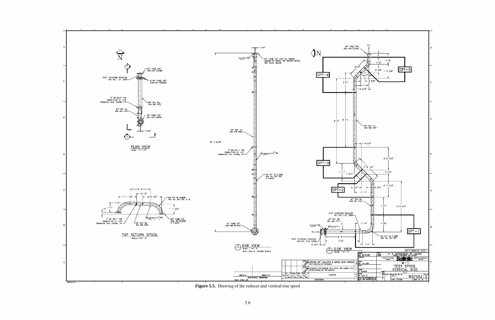
5.6
Figure 5.5. Drawing of the reducer and vertical-rise spool

5.7
Figure 5.6. Schematic of the GDPF pipe flow test section
Figure 5.7. Side view diagram of the GDPF pipe flow test arrangement
Figure 5.8. Top view diagram of the GDPF pipe flow test section

5.8
5.1 Piping and Test Spools
The piping used for the flow-loop system consists primarily of 3-inch, schedule-40, 304-stainless steel (with some recycled 316-stainless steel pieces). The spools used for this testing are described herein.
The pressure-drop measurements across the components of the gravity-feed and process-drain test
module, the jumper test module, the complex-geometry test module, and the reducer and vertical-rise test module were performed with a differential pressure transducer (DPT). The DPTs used are referred to as DPT-1, DPT-2, and so on according to their locations as shown in Figure 5.2 to Figure 5.5. The location of a modular component can be easily identified by counting its location starting from the first component of the test module and increasing in the flow direction. The count numbers correspond with the numbers following the abbreviation “DPT.” In this manner, a DPT can be easily associated with the modular component across which the DPT is taking measurements.
Figure 5.2 presents the drawing of the gravity-feed and process-drain test module. DPT-1 is used to
measure the pressure drop across the first modular component of a tee, followed downstream by DPT-2, DPT-3, DPT-4 and DPT-5 for measurements across the second, third, fourth, and fifth modular components, 90o 3D elbows. This test module is configured so that the slurry flows through modular components with a 1:50 downward slope (Figure 5.2 does not reflect this slope).
Figure 5.3 presents the drawing of the jumper test module. DPT-1 and DPT-3 are used to measure the pressure drop across the first and third modular components, 90o miter bends. The measurement with DPT-2 is performed for the second modular component, a 90o 3D elbow located between the two 90o miter bends. The jumper test module is configured so the slurry flows horizontally until the first 90o miter bend redirects it upward, a 90o 3D elbow returns it to horizontal flow, and the second 90o miter bend directs it once again to the vertical. Due to time constraints, the jumper test module was set up by connecting the jumper test module to the gravity-feed and process-drain test module in such a way that the slurry flow from the jumper test module entered into the gravity-feed and process-drain test module.
Figure 5.4 presents the drawing of the complex-geometry test module. DPT-1 is used to measure the pressure drop across the first modular component, a 90o 3D elbow, followed downstream by DPT-2 for measurement across the second modular component, a 90o 3D elbow combined with a 45o 3D elbow. The measurement across the third modular component, a combination of two 45o 3D elbows, is performed with DPT-3. Following DPT-3 downstream, DPT-4 and DPT-5 are used for the pressure-drop measurements across the fourth and fifth modular components, 90o 5D elbows.
The complex-geometry module was configured so that the slurry flow entered the first modular
component horizontally and was redirected vertically upward through the first component. The second modular component changed the flow direction from vertical to an upward slope 1:20 from horizontal. After passing through the third modular component with the 1:20 upward slope, the flow was redirected vertically downward through the fourth component. The fifth component changed the flow from vertically downward to horizontal. Figure 5.4 does not reflect the 1:20 slope between the exit of the 90 o 3D elbow (the second component) and the entrance of the 90 o 5D elbow (the fourth component).

5.9
Figure 5.5 presents the drawing of the reducer and vertical-rise test module. DPT-1 is used to
measure the pressure drop across the first modular component, a reducer combined with a 90o 3D elbow, followed downstream by DPT-2 and DPT-3 for measurements across the second and third modular components, which are 45o 3D elbows. The measurements across the fourth and fifth modular components, two 45o 3D elbows, are performed with DPT-4 and DPT-5.
The reducer and vertical-rise module was configured so the slurry flow entered the reducer
horizontally and underwent expansion and reduction before being redirected vertically upward through the 90o 3D elbow (Note: the reducer and 90o 3D elbow comprise the first modular component). This slurry flow remained in the upward direction through the rest of the components of this reducer and vertical-rise test module.
Figure 5.6 to Figure 5.8 present the diagrams of the 8-inch GDPF pipe flow test module. The slurry flow driven by the slurry pump is contained in the 50-gallon reservoir tank before it is introduced into the test section. The slurry flow is then driven by gravity from the slurry height in the reservoir tank through the first transparent section (labeled ‘Clear Section’ in Figure 5.6), then the four 90o 3D elbows (see Figure 5.8), and finally the second transparent section before it infuses into the 50-gallon receiving tank. The slurry height in the receiving tank is maintained below the pipe end that connected the receiving tank with a transfer pump to avoid interference from the slurry height in the receiving tank on the slurry flow. Three downward slopes of 1:125, 1:50, and 1:20 are used for the 8-inch GDPF pipe flow test module for three tests, respectively (see Figure 5.7).
5.2 Slurry Pump
The slurry pump is a Georgia Iron Works GIW 2X3LCC-M9 (LCC-M 50-230.2K M1). A picture of a similar pump is shown in Figure 5.9. The pump is driven by a 15-hp, 1800 rpm, totally enclosed fan-cooled 460-V electric motor produced by Reliance XEX as model P25G3316. This motor is connected to the pump by a belt drive. A Flowserve SL-C single cartridge flushless mechanical seal is used in this pump.
Figure 5.9. Photograph of Georgia Iron Works 2X3LCC Slurry Pump (Source: www.giwindustries.com)

5.10
5.3 Mixing Tank
The mixing tank is a standard four-baffle mixing tank with a 54-inch internal diameter. The maximum capacity of this tank is approximately 400 gallons. The tank is agitated by a 25-inch-diameter, 4-bladed pitched-blade impeller (4PBT45) driven by a 10-hp overhead electric motor manufactured by Philadelphia Mixers. At full speed, the system rotates at 155 rpm. A dip-tube system is used to feed and return the slurry from the test loop. A drawing of the mixing tank internal components is shown in Figure 5.10.
Figure 5.10. Schematic of Mixing Tank Internal Components
5.4 Flush System
The flush tank was a “U” stamped pressure vessel (National Board Number 18,365) rated to a maximum working pressure of 150 psig. The tank’s diameter is 4 ft and its capacity is 400 gallons. The tank is jacketed to allow for temperature control. The flush tank was augmented with a jet mixer system. A drawing of the flush tank’s internal components is shown in Figure 5.11.

5.11
Figure 5.11. Schematic of Flush Tank Internal Components
5.5 Data Acquisition System
The data acquisition system took temperature, flow, level, and pressure data from the flow loop and stored it in data files. The system was running National Instruments LabView software with a nominal sampling rate of 300 ms.
5.6 Differential Pressure Transducers
Rosemount 1151 differential pressure transducers (DPT) were used for the pressure-drop measurements across the components of the modular test section. The accuracy is 0.25% of the measurement within the calibrated span of 0 to 150 inches H2O differential. The pressure transducers were connected to the flow loop through open horizontal weldolet connectors. The open design of the

5.12
ports was selected over diaphragm systems to allow for greater pressure sensitivity. Since sediment was expected to fill these ports during operation, a differential-pressure port purge system was also installed. This system allowed the DPTs to be isolated from the flow loop. The differential-pressure ports were then cleaned by briefly flushing lines with high-pressure water. This purge process was implemented as needed throughout testing. Two transducers with differing pressure measurement ranges were connected to a pair of weldolet ports. This allowed for a broad range of pressure measurements to be taken.
5.7 Coriolis Meters
The Coriolis meters used during testing were Micro-Motion F-Series sensors designed for 3-inch, schedule-40 pipe and made of 316L stainless steel.
5.8 Video Camera Recorder
A Sony® video camera recorder, CCD-TRV138NTSC Hi8, was used for videotaping the slurry flow observation.

6.1
6.0 Test Procedure
Tests to determine the effects of the piping geometry on the critical pipeline velocity were performed
for the four test spools as described in Section 5. In these tests, the pressure drop was measured across each component of the test spool to evaluate critical velocities and velocities for avoiding deposition (VFAD). After the pressure-drop measurements, the experimental work was continued to test the flushing operation. The experiments to measure the pressure drop and to conduct the flush testing are referred to as “pressure-drop measurement and flush tests” herein. In addition to the pressure-drop measurement and flush tests, three downward pipe slopes of 1:125, 1:50, and 1:20 were used to inspect the particle sedimentation process in the 8-inch gravity-driven partially-filled (GDPF) pipe flow. This testing is referred to as “GDPF pipe flow tests” herein. This section presents the procedures of the pressure-drop measurement and flush tests and the GDPF pipe flow tests.
6.1 Procedure for Pressure-Drop Measurement and Flush Tests
In order to produce the pressure-drop distributions from which critical velocities and VFADs were obtained, pressure drop was measured across each component of the gravity-feed and process-drain test module, the jumper test module, the complex-geometry test module, and the reducer and vertical-rise test module. Along with the pressure drop, the flow rate (velocity), slurry density, slurry temperature, mixing and flush tank temperatures, water heater and chiller temperatures, flow-loop pressure drop, and air tank pressure were measured. After taking those measurements, the flushing operation was tested. The procedure for the pressure-drop measurements and the flush operation testing is outlined, as a sequence of steps, below. 1) Start the Data Acquisition System
The data acquisition system was started to record the pressure drop, flow rate (velocity), slurry density, slurry temperature, mixing and flush tank temperatures, water heater and chiller temperatures, flow-loop pressure drop, and air tank pressure.
2) Load Simulant for Testing
The simulant described in Section 4 was loaded into a rinsed and drained mixing vessel and flow loop. Tap water, to be used as the flush solution, was added to the flush vessel.
3) Homogenize Simulant
The mechanical agitator on the mixing vessel was started for solids homogenization. The mixing-vessel temperature control system was set to the appropriate value, nominally 25ºC.
4) Start Pipe Flow
The flow-loop pump was started with a target flow velocity of 7.5 or 8 ft/sec as specified by the cognizant test engineer. The Coriolis meters on the flow loop were used to verify this reading.

6.2
5) Confirm Homogenization
The mixing-vessel flow loop was operated to determine slurry density in the vessel via Coriolis flow meters. Agitator rotational rates were adjusted such that the solid-volume fractions were within 20% of the theoretical calculated values for complete homogenization, as well as to minimize the entrainment of air in the pipe loop.
6) Take Samples and Measure Rheological Properties
A grab sample was taken from the mixing vessel, and a flow curve (see Section 4) was measured. During the testing, this rheological property measurement and the DPT purging were performed frequently under the direction of the cognizant test engineer.
7) Determine Steady-State Condition
A flow rate was held constant for a minimum of 30 minutes before a steady-state condition was assumed. If the transient pressure signal indicated a trend after this 30-minute period, the flow was held constant until a steady state was determined by the cognizant test engineer.
The temperature of the slurry was held constant during this testing via automatic temperature control on the jacketed mixing vessel. The temperature was maintained within 10ºC of target temperature.
8) Decrease Flow rate
The flow rate was decreased in increments under the direction of the cognizant test engineer and Step 7 was repeated until reaching the minimum velocity specified by the cognizant test engineer.
9) Stop Flow The pump was then stopped with the line partially filled with sediment.
10) Switch to Flush Mode
Valves were reconfigured to operate in flush mode. This mode allowed for flow from the flush tank to go to the spent simulant vessel. The flush tank was filled with water, which was then driven through the system at the specified operating pressure.
11) Stop the Data Acquisition System
6.2 Procedure for GDPF Pipe Flow Tests
Three downward pipe slopes of 1:125, 1:50, and 1:20 were used to inspect the particle sedimentation process of the 8-inch GDPF pipe flow. In this subsection, the procedure for the GDPF pipe flow tests is outlined, as a sequence of steps, below.

6.3
1) Start the Data Acquisition System
The data acquisition system was started to record the flow rate (velocity), slurry density, slurry temperature, mixing and flush tank temperatures, water heater and chiller temperatures, and air tank pressure.
2) Load Simulant for Testing
The simulant described in Section 4 was loaded into a rinsed and drained mixing vessel and flow loop. Tap water, to be used as the flush solution, was added to the flush vessel.
3) Homogenize Simulant
The mechanical agitator on the mixing vessel was started for solids homogenization. The mixing-vessel temperature control system was set to the appropriate value, nominally 25ºC.
4) Start Pipe Flow
The flow-loop pump was started, under the direction of the cognizant test engineer, with a target flow velocity of 8 ft/sec. The Coriolis meters on the flow loop were used to verify this reading.
5) Confirm Homogenization
The mixing-vessel flow loop was operated to determine slurry density in the vessel via Coriolis flow meters. Agitator rotational rates were adjusted so the solid-volume fractions were within 20% of the theoretical calculated values for complete homogenization, as well as to minimize the entrainment of air in the pipe loop.
6) Take Samples and Measure Rheological Properties
A grab sample was taken from the mixing vessel, and a flow curve (see Section 4) was measured. During the testing, this rheological property measurement and the DPT purging were performed frequently under the direction of the cognizant test engineer.
7) Minimum 30-Minute Flow Run
The flow rate was held constant for a minimum of 30 minutes or as instructed by the cognizant test engineer.
During this time period, the slurry deposition process was observed through the transparent sections and inspected by inserting a hand through the open port on the test module; results were recorded in the Laboratory Record Book. Videotaping was performed under the direction of the cognizant test engineer.
6.4
The temperature of the slurry was held constant via automatic temperature control on the jacketed mixing vessel. The temperature was maintained within 10ºC of the target temperature.
8) Decrease Flow Rate The flow rate was decreased in increments under the direction of the cognizant test engineer and Step 7 was repeated until the cognizant test engineer instructed to stop the slurry pump. Videotaping was performed during changes in the flow rate.
9) Inspect Slurry Deposition
With no flow condition after the slurry pump was stopped, the slurry deposition process was inspected by observation through the transparent sections and the open port on the test module. In addition, the inspection was performed by inserting a hand through the open port on the test module. Results were recorded in the Laboratory Record Book.
10) Flush Modular Test Section
Under the direction of the cognizant test engineer, the modular test section was flushed with tap water.
12) Stop the Data Acquisition System

7.1
7.0 Critical Velocity and Velocity for Avoiding Deposition
Tests to determine the effects of the piping geometry on the slurry particle deposition were performed for the four test spools. The test spools included the following pipeline configurations: 1) gravity feed and process drain, 2) jumper, 3) complex geometry, and 4) reducer and vertical-rise. This section presents and discusses the results of the tests with these test modules.
7.1 Test Results
The pressure drop across each component of the gravity-feed and process-drain test module, the jumper test module, the complex geometry test module, and the reducer and vertical-rise test module was measured with a differential pressure transducer (DPT). The DPTs are referred to as DPT-1, DPT-2, and so on according to their locations (see Figure 5.2 to Figure 5.5). The location of the modular component can be easily identified by counting from the first component of the test module and increasing in the flow direction. The count numbers correspond to the numbers following the abbreviation “DPT.” In this manner, a DPT can be simply associated with the modular component across which the DPT is taking measurements.
As described in Subsection 5.1, the DPTs measure the pressure drop between the two pressure ports
on the test module components that have rising and falling slopes. Due to the density difference between the slurry flowing inside the pipeline of the modular components, and water inside the tubes that connect DPTs to the pressure ports on the modular components, the vertical distances between the two ports on the test module components cause the DPT readings to include the hydrostatic pressure due to gravity. This effect can be removed from the measured DPT data by adding (or subtracting, in the case of upward
flow) the correction factor c to (or from) the DPT readings, with
ghwaterSlurryc [7.1]
where Slurry is the slurry density
water is the water density
g is the acceleration due to gravity
h is the vertical distance between the pressure ports on the modular component To perform accurate DPT data corrections with Equation [7.1], the following items need to be
satisfied: (1) the accurate slurry densities inside the modular components are measured and (2) the DPT pressure tubes that connect the DPTs to the pressure ports on the modular components contain only water.
For this correction of the DPT data, the slurry density obtained with the Coriolis flow meter at a position well upstream of the modular test section was used. Therefore, it is expected that, in low velocity conditions, the density given by the Coriolis flow meter differs from the density at the pressure ports where the DPT measurements are performed, possibly due to particle settling. The inaccuracy of the density measurements is considered to cause uncertainty for the data analysis. In addition, high uncertainty is expected in the pressure measurements since the static pressure measured by a DPT was the

7.2
local static pressure in the immediate vicinity of the pressure ports which was considered to be different from the average pressure in the pipe cross section due to the complex flow structure produced by the geometry of the modular component. The high uncertainty in the density and pressure measurements is deemed to significant but no corrective method is available.
In this section, the measured pressure-drop values (DPT data) with and without the correction by
applying Equation [7.1] are presented. The uncorrected DPT data can provide only a qualitative description since these data include the hydrostatic pressure due to gravity. It is pointed out that the hydrostatic pressure due to gravity is not constant over a test run since the density changes as the flow velocity changes. For the corrected DPT data, due to the expected high uncertainty in the density and pressure data as discussed above, accurate quantitative analyses are also not available. The data analyses of this study provide only a qualitative description of the pressure drop characteristics across the test module components. Gravity-Feed and Process-Drain Test Module
Figure 7.1 presents the plots of the pressure-drop distributions as a function of pipeline velocity for
the data obtained with DPTs across every modular component of the gravity-feed and process-drain test module. In Figure 7.1, the uncorrected DPT data are given in the left column while the right column includes the corrected DPT data. The top plots of Figure 7.1 are for the data of the first test, the middle plots are for the data of the second test, a repetition of the first, and the bottom plots are for the data of the third test, another repetition. DPT-1 was used to measure the pressure drop across the first modular component, a tee, followed downstream by DPT-2, DPT-3, DPT-4 and DPT-5 for the measurements across the second, third, fourth, and fifth modular components, which were 90o 3D elbows (see Figure 5.2). This test module was configured so the slurry flowed through the modular components with a 1:50 downward slope (Figure 5.2 does not reflect this slope). The hydrostatic pressure due to the 1:50 slope is small. Therefore, the differences between uncorrected and corrected data for this test module are expected to be small.
The general characteristic of the distributions observed in Figure 7.1 is that, as the pipeline velocity
decreases from a maximum, the pressure-drop value across the modular components decreases to a minimum and then slightly increases while the pipeline velocity continues to decrease. In some cases, the minimum pressure-drop values are observed at the smallest velocities used for the tests (note: the smallest velocity used for the repeated third test was 2.5 ft/sec).
Practically, the fluctuations in the smooth curve lines of Figure 7.1 are considered to be caused by the
geometry of the modular components since they vary for the repeated tests. Thus, the pressure-drop distributions for the data obtained with DPT-2, DPT-3, and DPT-4, which were used for the measurements across the same fitting of the 90o 3D elbow, could be considered similar.
The data obtained by DPT-5, which measured the pressure difference over the fifth component, a 90o
3D elbow, deviates from the general characteristic of the pressure-drop and pipeline-velocity distribution, as the distribution includes a spike point at a velocity of 2.5 ft/sec. This spike in pressure drop is observed for the repeated second and third tests as well (note: the repeated tests were performed for selected pipeline velocities). As seen in Figure 7.1, the repeated third test did not take measurements for the pipeline velocities below 2.5 ft/sec; however, it is inferred that the same distribution trend would be

7.3
obtained for the third test as the first and second tests since all of the measured values agree with each other for these three test runs.
The cause of the spike in DPT-5 data produced is not certain, however it can be pointed out that the
low-pressure port of DPT-5 was located at the end point of the 90o 3D elbow where the slurry flow entered the straight section of the modular component, and was located on the inner side of the 90o elbow arc (see Figure 5.2). The slurry particles were considered to be more uniformly distributed in high-velocity flow due to the high momentum of flow turbulence. However, as the velocity decreased to about 3 ft/sec, the flow might enter the transition regime between turbulent and laminar flow. At the pipeline velocity of 3 ft/sec, flowing in the 90o elbow arc, the slurry particles might experience a larger centrifugal force than the longitudinal force given by the carrier fluid due to the reduction in fluid flow momentum. This might cause the higher concentration of particles in the outer side of the 90o elbow arc and the lower concentration in the inner side. Due to the lower particle density concentration, a significantly lower-than-average static pressure across the pipeline is expected in the vicinity of the lower-pressure DPT-5 port, which might produce the large spike in pressure differences for the pipeline velocity region from 2 to 3 ft/sec.
The critical velocity of the DPT-1 data for the first modular component of the tee was evaluated to be
3.5 ft/sec, which is markedly larger than those for the other modular components. The cause of this high critical velocity could be that expansion of the cross section area by the tee modular component reduced the slurry flow. Therefore, the slurry flow velocity in this tee section was lower than the pipeline velocity indicated by the Coriolis flow meter, and the particle settlement occurred at a pipeline flow velocity at which the slurry particles were suspended in the flow for the other modular components.
Large fluctuation is observed in all of the DPT data for the low velocity range. Due to the large
fluctuation in the DPT data, it is inconclusive that the J-curve profile (see Subsection 3.1) was obtained for the DPT data, except DPT-1 data, of the gravity-feed and process-drain test module. The geometry of the modular components is considered to be responsible for the large fluctuations. Since the locations of the pressure ports used for the pressure-drop measurements were near to the modular components, it is expected that the flow in the vicinities of the pressure ports were unstable and caused the large fluctuation in DPT data. In addition, formation of the unstable bed of particles may cause the large fluctuation in DPT data. For the velocity range lower than 3 ft/sec (2 ft/sec for DPT-5 data), the flow might become laminar and the unstable bed of particles might be formed on the bottom of the modular components. The particles that settled on the bottom of the modular component might be lifted up by the fluid flow and then settle again downstream in this velocity range.
The locations of the pressure ports near to the modular components and the formation of the unstable
particle bed are considered to cause the large fluctuation in pressure drop (even a negative value was measured) at these velocities, as seen in Figure 7.1 for the three test runs.

7.4
Un-corrected DPT Data (1st test run)
0.00
0.05
0.10
0.15
0.20
0.25
0.30
0 1 2 3 4 5 6 7 8 9
Velocity (fps)
Pre
ssu
re D
rop
(p
si)
DPT-1 DPT-2 DPT-3 DPT-4 DPT-5
Corrected DPT Data (1st test run)
0.00
0.05
0.10
0.15
0.20
0.25
0.30
0 1 2 3 4 5 6 7 8 9
Velocity (fps)
Pre
ssu
re D
rop
(p
si)
DPT-1 DPT-2 DPT-3 DPT-4 DPT-5
Un-corrected DPT Data (2nd test run)
-0.05
0.00
0.05
0.10
0.15
0.20
0.25
0.30
0 1 2 3 4 5 6 7 8 9
Velocity (fps)
Pre
ssu
re D
rop
(p
si)
DPT-1 DPT-2 DPT-3 DPT-4 DPT-5
Corrected DPT Data (2nd test run)
-0.05
0.00
0.05
0.10
0.15
0.20
0.25
0.30
0 1 2 3 4 5 6 7 8 9
Velocity (fps)
Pre
ssu
re D
rop
(p
si)
DPT-1 DPT-2 DPT-3 DPT-4 DPT-5
Un-corrected DPT Data (3rd test run)
0.00
0.05
0.10
0.15
0.20
0.25
0.30
0 1 2 3 4 5 6 7 8 9
Velocity (fps)
Pre
ssu
re D
rop
(p
si)
DPT-1 DPT-2 DPT-3 DPT-4 DPT-5
Corrected DPT Data (3rd test run)
0.00
0.05
0.10
0.15
0.20
0.25
0.30
0 1 2 3 4 5 6 7 8 9
Velocity (fps)
Pre
ssu
re D
rop
(p
si)
DPT-1 DPT-2 DPT-3 DPT-4 DPT-5
Figure 7.1. Plots of pressure drop vs. pipeline velocity for the gravity-feed and process-drain module. The left column is the uncorrected DPT data and the right column is the corrected DPT data.
The top plots are of the first test run, the middle are of the second test run, and the bottom are of the third test run. DPT-1 is the DPT used for the first modular component of the tee, followed downstream by DPT-2, DPT-3, DPT-4, and DPT-5 for the second, third, fourth and fifth components of the 90° 3D elbows, respectively.

7.5
Jumper Test Module
Figure 7.2 presents plots of the pressure-drop distributions as a function of the pipeline velocity for the data obtained with DPT-1, DPT-2, and DPT-3 for the jumper test module. In Figure 7.2, the uncorrected DPT data are given in the left column while the right column includes the corrected DPT data. The top plots of Figure 7.2 are for the data of the first test, the middle plots are for the data of the second test, a repetition of the first, and the bottom plots are for the data of the third test, another repetition. DPT-1 and DPT-3 were used to measure the pressure drop across the first and third modular components, 90o miter bends. The measurement with DPT-2 was performed for the second modular component, a 90o 3D elbow located between the two 90o miter bends (see Figure 5.3). The jumper test module is configured so the slurry flows horizontally until the first 90 o miter bend redirects it upward, a 90 o 3D elbow returns it to horizontal flow, and the second 90 o miter bend directs it once again to the vertical.
The general characteristic of the distribution for the data obtained with DPT-1 and DPT-3 is
analogous to that of the gravity-feed and process-drain module as presented in Figure 7.1, whereas the DPT-2 data present a drastically different distribution (negative values for the corrected DPT data). For both the uncorrected and corrected data from the DPT-1 and DPT-3 measurements, the minimum pressure-drop values are observed at the smallest velocities used for the tests.
For this jumper test module, the same port on the modular pipe was used to measure the pressure at
the low pressure port of DPT-1 and at the high pressure port of DPT-2. Likewise, the same port on the modular pipe was used to measure the pressure at the low pressure port of DPT-2 and at the high pressure port of DPT-3 (see Figure 5.3). It is seen that the DPT-2 measurement over the 90o 3D elbow indicates a significantly small gradient in the pressure-drop distribution with high fluctuation. The cause for this may be that the upstream flow entering the second modular component, the 90o 3D elbow, was extremely disturbed by the presence of the first modular component, a 90o miter bend. Due to the complex flow structure of high-intensity turbulence, the static pressure obtained by DPT-2 could not represent the average pressure of the cross section of the 90o 3D elbow at the location of the high pressure DPT-2 port, and the small gradient in pressure distribution for DPT-2 data could be produced. It seems the flow was regulated by going through the 90o elbow and less-disturbed flow entered the third modular component of the 90o miter bend. Thus, DPT-1 and DPT-3 could measure a similar pressure-drop distribution.
The high turbulence of the slurry flow generated by the presence of the 90o miter bends could explain
the large gradients in the pressure-drop distributions for the DPT-1 and DPT-3 data seen in Figure 7.2.

7.6
Un-corrected DPT Data (1st test run)
0.00
0.20
0.40
0.60
0.80
1.00
0 1 2 3 4 5 6 7 8 9
Velocity (fps)
Pre
ssu
re D
rop
(p
si)
DPT-1 DPT-2 DPT-3
Corrected DPT Data (1st test run)
-0.10
0.10
0.30
0.50
0.70
0.90
0 1 2 3 4 5 6 7 8 9
Velocity (fps)
Pre
ssu
re D
rop
(p
si)
DPT-1 DPT-2 DPT-3
Un-corrected DPT Data (2nd test run)
0.00
0.20
0.40
0.60
0.80
1.00
0 1 2 3 4 5 6 7 8 9
Velocity (fps)
Pre
ssu
re D
rop
(p
si)
DPT-1 DPT-2 DPT-3
Corrected DPT Data (2nd test run)
-0.10
0.10
0.30
0.50
0.70
0.90
0 1 2 3 4 5 6 7 8 9
Velocity (fps)
Pre
ssu
re D
rop
(p
si)
DPT-1 DPT-2 DPT-3
Un-corrected DPT Data (3rd test run)
0.00
0.20
0.40
0.60
0.80
1.00
0 1 2 3 4 5 6 7 8 9
Velocity (fps)
Pre
ssu
re D
rop
(p
si)
DPT-1 DPT-2 DPT-3
Corrected DPT Data (3rd test run)
-0.10
0.10
0.30
0.50
0.70
0.90
0 1 2 3 4 5 6 7 8 9
Velocity (fps)
Pre
ssu
re D
rop
(p
si)
DPT-1 DPT-2 DPT-3
Figure 7.2. Plots of pressure drop vs. pipeline velocity for the jumper module. The left column is the uncorrected DPT data and the right column is the corrected DPT data.
The top plots are of the first test run, the middle are of the second test run and the bottom are of the third test run. DPT-1 is the DPT used for the first modular component of the 90° miter bend, followed downstream by DPT-2 and DPT-3 for the second and third components, the 90° 3D elbow and the 90° miter bend, respectively.

7.7
Complex-Geometry Test Module Figure 7.3 presents the plots of the pressure-drop distributions as a function of pipeline velocity for
the data obtained with DPTs across every modular component of the complex-geometry test module. In Figure 7.3, the uncorrected DPT data are given in the left column while the right column includes the corrected DPT data. The top plots of Figure 7.3 are for the data of the first test, the middle plots are for the data of the second test, a repetition of the first, and the bottom plots are for the data of the third test, another repetition. DPT-1 was used to measure the pressure drop across the first modular component, a 90o 3D elbow, followed downstream by DPT-2 for the measurement across the second modular component, a 90o 3D elbow combined with a 45o 3D elbow. The measurement across the third modular component, a combination of two 45o 3D elbows, was performed with DPT-3. Following DPT-3 downstream, DPT-4 and DPT-5 were used for the pressure-drop measurements across the fourth and fifth modular components, 90o 5D elbows (see Figure 5.4).
This complex-geometry module was configured so the slurry flow entered the first modular
component horizontally and was redirected vertically upward through the first component. The second modular component changed the flow direction from vertical to an upward slope 1:20 from horizontal. After passing through the third modular component with the 1:20 upward slope, the flow was redirected vertically downward through the fourth component. The fifth component changed the flow from vertically downward to horizontal. Figure 5.4 does not reflect the 1:20 slope between the exit of the 90 o 3D elbow (the second component) and the entrance of the 90 o 5D elbow (the fifth component).
Figure 7.3 shows that the pressure-drop distributions for the uncorrected DPT-4 and DPT-5 data are
significantly different from those for the corrected DPT-4 and DPT-5 data. This is because the pressure-drop measurements were performed by connecting the high (or low) DPT ports to the low (or high) pressure ports on these modular components. For the flow in the downward direction with the regular DPT connection setup, the hydrostatic pressure due to gravity causes a DPT to measure a negative value. The reverse DPT connection setup for the DPT-4 and DPT-5 were employed since the hydrostatic pressures due to gravity became adversely larger than the pressure-drop values across modular components in the low velocity region due to the large vertical distances between pressure ports as the negative values became lower than the minimum negative value (-0.169 psig) that DPT-4 and DPT-5 could measure. The DPT-4 and DPT-5 data obtained with the reverse DPT connections were corrected by reversing the sign after applying Equation [7.1] (subtracting the hydrostatic pressure due to gravity from measured DPT-4 and DPT-5 data). Plots in the right column of Figure 7.3 show the correct pressure-drop distributions.
Figure 7.3 shows that, for the uncorrected DPT data, the minimum pressure-drop values are observed
at the smallest velocities used for the tests in most cases (see the next subsection for a detailed discussion of critical velocities). For the corrected DPT data, Figure 7.3 shows the same general characteristic of the pressure-drop distribution as seen for the gravity-feed and process-drain test module. The data obtained with DPT-4 and DPT-5 show the same spike as seen in the DPT-5 data for the gravity-feed and process-drain test module. As in the case of the gravity-feed and process-drain module, the low pressure port of DPT-5 of this complex-geometry test module was located at the end point of the 90o 5D elbow where the slurry flow enters the straight section of the modular component (see Figure 5.4). The DPT-5 low-pressure port of this complex geometry test module was located at the end point of the 90o 5D elbow, at the height of the central axis of the pipe, while the location of the DPT-5 low pressure port of the gravity-

7.8
feed and process-drain test module was on the inner side of the 90o elbow arc. Regardless of this difference, it is rational that the same description used for the spike in the gravity-feed and process-drain test module data applies to the spike in DPT-5 data for this complex-geometry test module.
The low-pressure port of DPT-4 was located 3 inches downstream of the end point of the 90o 5D
elbow. It is conjectured that this difference in the low-pressure port location caused the low magnitude of the spike for DPT-4 data. It is interesting to point out that the spike occurred at the pipeline velocity of 2.5 ft/sec for all of these data.
The pressure-drop distribution for the corrected DPT-3 data is higher than for the other corrected DPT
data. The cause of the higher pressure-drop distribution for corrected DPT-3 data is not certain. It is considered possible that the second modular component could produce high intensity turbulence flow as the flow direction was changed from the vertical to an upward 1:20 slope from horizontal by the 90o 3D elbow, and then the slurry flowed through the 45o 3D elbow with a 1:20 slope (see Figure 5.4). This high intensity turbulence flow could cause a high pressure field in the area where the DPT-2 low pressure port and the DPT-3 high pressure port were located (the distance between the DPT-2 low pressure port and the DPT-3 high pressure port is about 10 inches). The turbulence intensity of this flow is considered to be reduced as the slurry flowed though the third modular component, a combination of two 45o 3D elbows, which could reduce the pressure at the DPT-3 low pressure port. Thus, the high pressure at the DPT-3 high pressure port and the low pressure at the DPT-3 low pressure port could be used to explain the high pressure-drop distribution for corrected DPT-3 data. In addition, the high pressure at the DPT-2 low pressure port could cause the low pressure-drop distribution for corrected DPT-2 data.
It is also pointed out that, as seen in Figure 7.3 for the corrected DPT data, large values of the
correction factor c were used for data correction except in the case of DPT-3 data. Therefore, it is
considered that data corrections were performed with high uncertainty, except in the case of DPT-3 data,
as the large values of correction factor c could account for high uncertainty.

7.9
Un-corrected DPT Data (1st test run)
0.00
0.10
0.20
0.30
0.40
0.50
0.60
0 1 2 3 4 5 6 7 8 9
Velocity (fps)
Pre
ssu
re D
rop
(p
si)
DPT-1 DPT-2 DPT-3 DPT-4 DPT-5
Corrected DPT Data (1st test run)
0.00
0.10
0.20
0.30
0.40
0.50
0.60
0 1 2 3 4 5 6 7 8 9
Velocity (fps)
Pre
ssu
re D
rop
(p
si)
DPT-1 DPT-2 DPT-3 DPT-4 DPT-5
Un-corrected DPT Data (2nd test run)
0.00
0.10
0.20
0.30
0.40
0.50
0.60
0 1 2 3 4 5 6 7 8 9
Velocity (fps)
Pre
ssu
re D
rop
(p
si)
DPT-1 DPT-2 DPT-3 DPT-4 DPT-5
Corrected DPT Data (2nd test run)
0.00
0.10
0.20
0.30
0.40
0.50
0.60
0 1 2 3 4 5 6 7 8 9
Velocity (fps)
Pre
ssu
re D
rop
(p
si)
DPT-1 DPT-2 DPT-3 DPT-4 DPT-5
Un-corrected DPT Data (3rd test run)
0.00
0.10
0.20
0.30
0.40
0.50
0.60
0 1 2 3 4 5 6 7 8 9
Velocity (fps)
Pre
ssu
re D
rop
(p
si)
DPT-1 DPT-2 DPT-3 DPT-4 DPT-5
Corrected DPT Data (3rd test run)
0.00
0.10
0.20
0.30
0.40
0.50
0.60
0 1 2 3 4 5 6 7 8 9
Velocity (fps)
Pre
ssu
re D
rop
(p
si)
DPT-1 DPT-2 DPT-3 DPT-4 DPT-5
Figure 7.3. Plots of pressure drop vs. pipeline velocity for the complex geometry module. The left column is uncorrected DPT data and the right column is corrected DPT data. The top
plots are of the first test run, the middle are of the second test run and the bottom are of the third test run. DPT-1 is the DPT used for the first modular component, a 90° 3D elbow, followed downstream by DPT-2 for the second component, a 90° 3D elbow combined with a 45° 3D elbow, followed by DPT-3 for the third component, a combination two 45° 3D elbows. Following DPT-3 downstream are DPT-4 and DPT-5 for the fourth and fifth components, two 90° 5D elbows.

7.10
Reducer and Vertical-Rise Test Module
Figure 7.4 presents plots of the pressure-drop distributions as a function of pipeline velocity for the
data obtained with DPTs across every modular component of the reducer and vertical-rise test module. In Figure 7.4, the uncorrected DPT data are given in the left column while the right column includes corrected DPT data. The top plots of Figure 7.4 are for data from the first test, the middle plots are for data from the second test, a repetition, and the bottom plots are for data from the third test, another repetition. DPT-1 was used to measure the pressure drop across the first modular component, a reducer combined with a 90o 3D elbow, followed downstream by DPT-2 and DPT-3 for measurements across the second and third modular components, two 45o 3D elbows. The measurements across the fourth and fifth modular components, 45o 3D elbows, were performed with DPT-4 and DPT-5 (see Figure 5.5).
This reducer and vertical-rise module was configured so the slurry flow entered the reducer
horizontally and underwent expansion and reduction before the flow was redirected vertically upward through the 90o 3D elbow (Note: the reducer and 90o 3D elbow comprise the first modular component). The slurry flow remained in the upward direction through the remaining components of this reducer and vertical-rise test module.
Once again it is pointed out that fluctuations in the smooth curves of Figure 7.4 are considered to be
caused by the geometry of the modular components since they vary in the repeated tests. General characteristics of the pressure-drop distribution seen in Figure 7.4 are consistent with those of the gravity-feed and process-drain test module, the jumper test module, and the complex-geometry test module. For the uncorrected DPT data, Figure 7.4 shows that minimum pressure-drop values are observed at the smallest velocities used for the tests in most cases (see the next subsection for a detailed discussion of critical velocities).
It is expected that slurry flow would decelerate as it enters the reducer and accelerate on exit due to
the expansion and reduction in area of the reducer. Therefore, the slowed slurry flow inside the 4-inch-diameter reducer resulted in a higher static pressure where the high-pressure port of DPT-1 was located. In addition, it is expected that the slurry flow inside the reducer could undergo slurry particle settlement at the pipeline velocity at which the particles were suspended in the flow. This slurry flow structure could explain the high gradient in the pressure-drop distribution for data obtained with DPT-1 as the lower pressure port was located on the 3-inch diameter pipeline (see both the uncorrected and corrected DPT-1 data in Figure 7.4).
The corrected DPT data in Figure 7.4 shows that the magnitude of the pressure-drop distribution for
the DPT-2 data is half of that for DPT-3 data for the higher-velocity region, even though both the DPT-2 and DPT-3 data were measured for 45o 3D elbows. DPT-2 measured the pressure drop across the first 45o 3D elbow, followed downstream by DPT-3 which measured the pressure drop across the second 45o 3D elbow. The distance between the low-pressure port of DPT-2 and the high-pressure port of DPT-3 was about 8 inches. The flow entered the first 45o 3D elbow from a straight pipe section and became high intensity turbulent through the elbow for higher velocities. Since the lower pressure port was located downstream of the elbow, it is possible that turbulence caused a high-pressure field in the vicinity of the lower pressure port of DPT-2. The pressure of the DPT-2 lower pressure port could increase by

7.11
increasing the turbulence intensity as the velocity increased, which could result in the low pressure-drop distribution for DPT-2 data for the high-velocity region, as the higher pressure port could measure the pressure of less turbulent flow since the DPT-2 higher pressure port was located on the straight pipe section upstream of the elbow.
Since the high-pressure port of DPT-3 was located only 8 inches from the low pressure-port of DPT-
2, the high-turbulence static pressure could be measured in the vicinity of the DPT-3 high-pressure port, which could result in the high pressure-drop distribution for DPT-3 data, as the low-pressure port of DPT-3 was located on the straight pipe section downstream of the second 45o 3D elbow.
The fourth modular component for DPT-4 was composed of two 45o 3D elbows, and was longer than
the third modular component, a single 45o 3D elbow for DPT-3. However, Figure 7.4 presents similar pressure-drop distributions for both DPT-3 and DPT-4 corrected data. The two combined 45o 3D elbows of the fourth modular component were actually followed by a 90o 5D elbow 5 inches downstream of the low-pressure port of DPT-4. Therefore, a high static pressure field could be expected in the vicinity of the DPT-4 low-pressure port due to the presence of the 90o 5D elbow, which could result in a lower pressure drop than that of the two combined 45o 3D elbows in the absence of the 90o 5D elbow.
In Figure 7.4, the data obtained with DPT-5 show a low gradient in the pressure-drop distribution and, for corrected DPT-5 data, high pressure-drop values in the pressure-drop distribution are observed. For the fifth modular component of the reducer and vertical-rise test module, the DPT-4 low-pressure port was used for the DPT-5 low-pressure port as well. Therefore, the DPT-5 low-pressure port could measure comparatively high static pressure due to the presence of the 90o 5D elbow. The DPT-5 high-pressure port was located downstream of the fourth modular component, a 45o 3D elbow. This elbow could produce a higher-pressure field due to turbulence in the vicinity of the DPT-5 high-pressure port. The pressure at the DPT-5 higher port might remain comparatively high at the lower velocities due to the turbulence produced by the fourth modular component of a 45o 3D elbow and might result in the high pressure-drop values in the pressure-drop distribution of the low gradient.

7.12
Un-corrected DPT Data (1st rest run)
0.00
0.20
0.40
0.60
0.80
1.00
0 1 2 3 4 5 6 7 8 9
Velocity (fps)
Pre
ssu
re D
rop
(p
si)
DPT-1 DPT-2 DPT-3 DPT-4 DPT-5
Corrected DPT Data (1st test run)
0.00
0.20
0.40
0.60
0.80
1.00
0 1 2 3 4 5 6 7 8 9
Velocity (fps)
Pre
ssu
re D
rop
(p
si)
DPT-1 DPT-2 DPT-3 DPT-4 DPT-5
Un-corrected DPT Data (2nd test run)
0.00
0.20
0.40
0.60
0.80
1.00
0 1 2 3 4 5 6 7 8 9
Velocity (fps)
Pre
ssu
re D
rop
(p
si)
DPT-1 DPT-2 DPT-3 DPT-4 DPT-5
Corrected DPT Data (2nd test run)
0.00
0.20
0.40
0.60
0.80
1.00
0 1 2 3 4 5 6 7 8 9
Velocity (fps)
Pre
ssu
re D
rop
(p
si)
DPT-1 DPT-2 DPT-3 DPT-4 DPT-5
Un-corrected DPT Data (3rd test run)
0.00
0.20
0.40
0.60
0.80
1.00
0 1 2 3 4 5 6 7 8 9
Velocity (fps)
Pre
ssu
re D
rop
(p
si)
DPT-1 DPT-2 DPT-3 DPT-4 DPT-5
Corrected DPT Data (3rd test run)
0.00
0.20
0.40
0.60
0.80
1.00
0 1 2 3 4 5 6 7 8 9
Velocity (fps)
Pre
ssu
re D
rop
(p
si)
DPT-1 DPT-2 DPT-3 DPT-4 DPT-5
Figure 7.4. Plots of pressure drop vs. pipeline velocity for the reducer and vertical-rise module. The left column is the uncorrected DPT data and the right column is the corrected DPT data.
The top plots are of the first test run, the middle are of the second test run and the bottom are of the third test run. DPT-1 is the DPT used for the first modular component, a reducer combined with a 90° 3D elbow, followed downstream by DPT-2 and DPT-3 in that order for the second and third components, 45° 3D elbows. Following DPT-3 downstream are DPT-4 and DPT-5 used for the fourth component, two 45° 3D elbows, and the fifth component, a 45° 3D elbow, respectively.

7.13
7.2 Discussion
The pressure drop across each component of the test module spool was measured and Figure 7.1 to Figure 7.4 present the measured pressure-drop distributions as a function of the pipeline velocity for both uncorrected and corrected DPT data. From the pressure-drop versus pipeline-velocity distributions for the uncorrected DPT data, the minima of the pressure-drop values were found with Microsoft Excel spreadsheet function “MIN,” and function “VLOOKUP” was used to find velocities corresponding to the obtained minimum pressure-drop values, except the cases of the fourth and fifth components of the complex-geometry module test. For the fourth and fifth components of the complex-geometry module test, function “MAX” was used to find the maxima of the pressure-drop values, and function “VLOOKUP” was used to find velocities corresponding to the obtained maximum pressure-drop values. The evaluated velocities are reported as “critical velocities” herein.
The critical velocities evaluated from uncorrected DPT data for all of the modular components for
each test run are summarized in Table 7.1. The critical velocity for a straight horizontal pipe was evaluated and reported by Poloski et al. (2008); Table 7.1 includes the critical velocity for a straight horizontal pipe for comparison. The critical velocities reported in Table 7.1 were based on the critical velocity definition used by Poloski et al. (2008). However, it is seen in Figure 7.1 to Figure 7.4 that pressure-drop-versus-velocity curves do not have a definite profile of the J-curve used to unambiguously determine the critical velocity as used by Poloski et al. (2008) (see Figure 3.1). As seen in Table 7.1, the critical velocities correspond in most cases to the smallest velocities used in the tests. The smallest velocities obtained need not to be the critical velocities since the J-curve profile could not be obtained. The uncorrected DPT data include the hydrostatic pressure due to gravity, as discussed in Subsection 7.1, which is not constant over a test run because density changes as the flow velocity changes. Pressures were considered to be measured with high uncertainty due to the complex flow structure produced by the geometry of the modular component. High uncertainty in uncorrected DPT data is seen from high fluctuation in Figure 7.1 to Figure 7.4 and makes it very difficult to determine the critical velocity. Therefore it is not certain that critical velocities were evaluated from the DPT data obtained.
For the gravity-feed and process-drain module test, the critical velocities for the first modular
component, a tee, are 3.5 ft/sec. This high critical velocity could be due to expansion of the cross-sectional area of the tee reducing the slurry flow, which resulted in lower slurry flow velocity in this tee section than the pipeline velocity indicated by the Coriolis flow meter, and sedimentation occurred at a pipeline flow velocity at which slurry particles were suspended in the flow for the other modular components. The critical velocity of 3.5 ft/sec evaluated for the fifth component, a 90o 3D elbow, for the repeated third test run, was because the measurement was not performed for velocities less than 2.5 ft/sec and this value of 3.5 ft/sec is not considered to be a critical velocity as the J-curve obtained was incomplete. The critical velocity of 2.5 ft/sec for the second, third, and fourth components for the repeated third test was the smallest velocity used for this test run. Except for the first modular component, a tee, all modular components of the gravity-feed and process-drain test module present critical velocities lower than those evaluated for a straight horizontal pipe.
For the jumper module test, comparatively higher critical velocities were evaluated for the second
component, a 90o 3D elbow, for the second test run. However, as discussed in Subsection 7.1, it is considered that complex flow structure due to high-intensity turbulence caused high fluctuation in the

7.14
pressure data for the second component, a 90o 3D elbow and it is indeterminate whether the critical velocity is obtained for the second component. The critical velocities (smallest velocities) obtained for the first and third components of 90o miter bend are lower than those evaluated for a straight horizontal pipe.
For the complex-geometry module test, the critical velocities evaluated for all modular components
are lower than those evaluated for the straight horizontal pipe. It is indeterminate whether the smallest velocities in Table 7.1 for the complex-geometry test module are critical velocities or merely smallest velocities due to high uncertainty in the DPT data.
For the reducer and vertical-rise module test, the data obtained for the fifth modular component, a 45o
elbow, present high critical velocities of 3.5 ft/sec for the first test and 2.5 ft/sec for the third test. A low gradient in the pressure-drop distribution was obtained for this modular component, and the fluctuation in DPT-5 data is high compared with this low distribution gradient. The low gradient of the pressure-drop distribution and the high fluctuation make it difficult to accurately predict the critical velocity. The configuration of this test module suggests that slurry-particle settling inside this modular component is very unlikely to occur and the obtained high values of the critical velocity for this modular component are highly unrealistic.
It is found that the critical velocities evaluated for all components of the reducer and vertical-rise test module except for the fifth modular component, a 45o elbow, are lower than those evaluated for a straight horizontal pipe. Except for the first component, a reducer combined with a 90o 3D elbow, the geometry of the reducer and vertical-rise test module strongly suggests that the critical velocities in Table 7.1 for the reducer and vertical-rise test module are smallest velocities used in these test runs.
In addition to the critical velocity, the velocity for avoiding deposition (VFAD) is reported in Table
7.1. As discussed above, due to the high fluctuations, it is difficult to determined critical velocities since a definite profile of the J-curve was not obtained in Figure 7.1 through Figure 7.4. The high uncertainty makes it difficult to use the evaluated critical velocities for the accurate prediction of particle deposition. Therefore, VFADs are used to provide velocities at which it is assured that no particle deposition occurs.
In Table 7.1, the obtained VFADs are reported as velocity ranges where slurry flow does not undergo
particle deposition. The VFADs were selected from Figure 7.1 through Figure 7.4 (see Subsection 3.1 for the determination of VFAD). As seen in Table 7.1, the VFADs for the second modular component, a 90o 3D elbow, of the jumper test module and for the second and fifth modular components, a 45o 3D elbow, of the reducer and vertical-rise test module were undetermined due to the high uncertainty (see Subsection 7.1)
Table 7.2 through Table 7.5 include uncorrected pressure drops, corrected pressure drops, densities
measured at a point upstream of the modular test section, and densities measured at a point downstream of the modular test section. These values correspond to the smallest VFADs reported herein. In addition, included in Table 7.2 through Table 7.5 are Bingham yield stresses, Bingham consistencies, and ranges of Reynolds numbers used for each test run. The Reynolds number of about 4100 for non-Newtonian fluids may be in laminar or transition. The Reynolds numbers were calculated with:

7.15
yconsistenc
Slurry DV
Re [7.2]
where Slurry is the slurry density
V is the pipeline velocity D is the pipe internal diameter of 3.068 inches
yconsistenc is the Bingham consistency.
It is pointed out that all Reynolds numbers reported are based on the nominal pipe size of 3 inches
(3.068 inches ID) and this characteristic dimension of 3.068 inches does not properly apply to the first modular component, a tee, of the gravity-feed and process-drain test module and the first modular component, a reducer and a 90o 3D elbows, of the reducer and vertical-rise test module.

7.16
Table 7.1. Critical velocity and VFAD evaluated from the uncorrected DPT data
Evaluated Critical Velocities of Modular Components (ft/sec)
Test Spool
DPT # Component Run
1 Run
2 Run
3
Range of Velocity for Avoiding Deposition
(VFAD) (ft/sec)
Critical Velocity of
Straight Pipe (ft/sec)
1 Tee 3.5 3.5 3.5 >= 4.0
2 90o 3D Elbow 2.5 1.5 2.5^ >= 3.5
3 90o 3D Elbow 2.0 2.0 2.5^ >= 3.5
4 90o 3D Elbow 1.5^ 2.0 2.5^ >= 3.5
Gravity Feed and
Process Drain
5 90o 3D Elbow 2.0 1.0^ 3.5 >= 3.5
1 90o Miter Bend 0.5^ 1.0^ 0.5^ >= 2.0
2 90o 3D Elbow 0.5^ 3.0 0.5^ * Jumper
3 90o Miter Bend 0.5^ 1.0^ 0.5^ >= 2.0
1 90o 3D Elbow 1.0 1.0^ 0.5^ >= 3.0
2 90o + 45o 3D Elbows 0.5^ 1.0^ 0.5^ >= 3.0
3 45o + 45o 3D Elbows 1.0 1.0^ 0.5^ >= 3.0
4 90o 5D Elbow 1.0 1.0^ 1.5 >= 3.5
Complex Geometry
5 90o 5D Elbow 1.5 1.0^ 1.5 >= 3.5
1 Reducer + 90o 3D
Elbow 1.5^ 1.0^ 1.5^ >= 3.0
2 45o 3D Elbow 1.5^ 1.0^ 1.5^ *
3 45o 3D Elbow 1.5^ 1.0^ 1.5^ >= 3.0
4 45o + 45o 3D Elbows 1.5^ 1.0^ 1.5^ >= 3.0
Reducer and
Vertical Rise
5 45o 3D Elbow 3.5 1.0^ 2.5 *
2.7
^ This is the velocity corresponding to the smallest measured pressure drop: however, this value needs not necessarily to be critical velocity as the entire J-curve could not be obtained.
* VFADs for these components were undetermined due to high uncertainties in the data.

7.17
Table 7.2. Pressure drop, density, yield stress, consistency, and Reynolds number for the gravity-feed and process drain module test
Gravity Feed and Process Drain
Tee 90o 3D Elbow 90o 3D Elbow 90o 3D Elbow 90o 3D Elbow Run1 Run2 Run3 Run1 Run2 Run3 Run1 Run2 Run3 Run1 Run2 Run3 Run1 Run2 Run3
Velocity for Avoiding
Deposition (VFAD) (ft/sec)
4.0 4.0 4.0 3.5 3.5 3.5 3.5 3.5 3.5 3.5 3.5 3.5 3.5 3.5 3.5
Uncorrected Pressure Drop (psi) at VFAD
0.037 0.034 0.035 0.050 0.049 0.048 0.045 0.025 0.041 0.032 0.034 0.033 0.057 0.050 0.053
Corrected Pressure Drop (psi) at VFAD
0.044 0.041 0.042 0.062 0.061 0.060 0.058 0.037 0.053 0.044 0.046 0.046 0.066 0.059 0.062
Density* (g/mL) at VFAD
1.403 1.403 1.402 1.403 1.402 1.402 1.403 1.402 1.402 1.403 1.402 1.402 1.403 1.402 1.402
Density** (g/mL) at VFAD
1.397 1.396 1.395 1.398 1.397 1.396 1.398 1.397 1.396 1.398 1.397 1.396 1.398 1.397 1.396
Bingham Yield Stress (Pa)
2.97 2.82 3.07 2.97 2.82 3.07 2.97 2.82 3.07 2.97 2.82 3.07 2.97 2.82 3.07
Bingham Consistency (cP)
7.16 7.82 6.80 7.16 7.82 6.80 7.16 7.82 6.80 7.16 7.82 6.80 7.16 7.82 6.80
Range of Reynolds
numbers used***
6800^ ~
37100^
4100^ ~
33900^
12100^ ~
39000^
6800 ~
37100
4100 ~
33900
12100 ~
39000
6800 ~
37100
4100 ~
33900
12100 ~
39000
6800 ~
37100
4100 ~
33900
12100 ~
39000
6800 ~
37100
4100 ~
33900
12100 ~
39000
^ Reynolds numbers are based on the nominal pipe size of 3 inches (3.068 inches ID).
* The density measurements were taken at a point upstream of the modular test section.
** The density measurements were taken at a point downstream of the modular test section.
*** Reynolds number of about 4100 for a non-Newtonian fluid may be in laminar or transition.

7.18
Table 7.3. Pressure drop, density, yield stress, consistency, and Reynolds number for the jumper module test
Jumper
90o Miter Bend 90o 3D Elbow 90o Miter Bend Run1 Run2 Run3 Run1 Run2 Run3 Run1 Run2 Run3 Velocity for Avoiding
Deposition (VFAD) (ft/sec)
2.0 2.0 2.0 ***** ***** ***** 2.0 2.0 2.0
Uncorrected Pressure Drop (psi) at VFAD
0.223 0.202 **** ***** ***** ***** 0.279 0.273 ****
Corrected Pressure Drop (psi) at VFAD
0.105 0.085 **** ***** ***** ***** 0.075 0.070 ****
Density* (g/mL)
at VFAD 1.357 1.355 **** ***** ***** ***** 1.357 1.355 ****
Density** (g/mL)
at VFAD 1.356 1.351 **** ***** ***** ***** 1.356 1.351 ****
Bingham Yield Stress
(Pa) 2.83 2.79 2.45 2.83 2.79 2.45 2.83 2.79 2.45
Bingham Consistency
(cP) 7.40 6.60 6.23 7.40 6.60 6.23 7.40 6.60 6.23
Range of Reynolds numbers used***
2100 ~
35100
4700 ~
39300
2400 ~
41500
2100 ~
35100
4700 ~
39300
2400 ~
41500
2100 ~
35100
4700 ~
39300
2400 ~
41500
* The density measurements were taken at a point upstream of the modular test section.
** The density measurements were taken at a point downstream of the modular test section.
*** Reynolds number of about 4100 for a non-Newtonian fluid may be in laminar or transition.
**** Pressure drops and densities were not available at VFAD of 2 (ft/sec) for Run 3 since the testing was not performed at this velocity.
***** VFADs for 90o 3D Elbow were undetermined due to high uncertainties in the data.

7.19
Table 7.4. Pressure drop, density, yield stress, consistency, and Reynolds number for the complex geometry module test
Complex Geometry
90o 3D Elbow 90o + 45o 3D Elbows 45o + 45o 3D Elbows 90o 5D Elbow 90o 5D Elbow Run1 Run2 Run3 Run1 Run2 Run3 Run1 Run2 Run3 Run1 Run2 Run3 Run1 Run2 Run3
Velocity for Avoiding
Deposition (VFAD) (ft/sec)
3.0 3.0 3.0 3.0 3.0 3.0 3.0 3.0 3.0 3.5 3.5 3.5 3.5 3.5 3.5
Uncorrected Pressure Drop (psi) at VFAD
0.291 0.290 **** 0.305 0.304 **** 0.105 0.102 **** 0.281 **** 0.267 0.258 **** 0.275
Corrected Pressure Drop (psi) at VFAD
0.045 0.044 **** 0.045 0.045 **** 0.074 0.071 **** 0.046 **** 0.059 0.065 **** 0.047
Density* (g/mL) at VFAD
1.333 1.332 **** 1.333 1.332 **** 1.333 1.332 **** 1.335 **** 1.333 1.335 **** 1.333
Density** (g/mL) at VFAD
1.330 1.328 **** 1.330 1.328 **** 1.330 1.328 **** 1.331 **** 1.329 1.331 **** 1.329
Bingham Yield Stress (Pa)
2.71 2.85 2.75 2.71 2.85 2.75 2.71 2.85 2.75 2.71 2.85 2.75 2.71 2.85 2.75
Bingham Consistency (cP)
5.72 6.30 5.74 5.72 6.30 5.74 5.72 6.30 5.74 5.72 6.30 5.74 5.72 6.30 5.74
Range of Reynolds
numbers used***
2600 ~
44000
4800 ~
40000
2500 ~
41100
2600 ~
44000
4800 ~
40000
2500 ~
41100
2600 ~
44000
4800 ~
40000
2500 ~
41100
2600 ~
44000
4800 ~
40000
2500 ~
41100
2600 ~
44000
4800 ~
40000
2500 ~
41100
* The density measurements were taken at a point upstream of the modular test section.
** The density measurements were taken at a point downstream of the modular test section.
*** Reynolds number of about 4100 for a non-Newtonian fluid may be in laminar or transition.
**** Pressure drops and densities were not available at VFAD of 3 (ft/sec) for Run 3 and VFAD of 3.5 (ft/sec) for Run 2 since the testing was not performed at these velocities.

7.20
Table 7.5. Pressure drop, density, yield stress, consistency, and Reynolds number for the reducer and vertical rise module test
Reducer and Vertical Rise
Reducer+90o 3D Elbow 45o 3D Elbow 45o 3D Elbow 45o+45o 3D Elbows 45o 3D Elbow Run1 Run2 Run3 Run1 Run2 Run3 Run1 Run2 Run3 Run1 Run2 Run3 Run1 Run2 Run3
Velocity for Avoiding
Deposition (VFAD) (ft/sec)
3.0 3.0 3.0 ***** ***** ***** 3.0 3.0 3.0 3.0 3.0 3.0 ***** ***** *****
Uncorrected Pressure Drop (psi) at VFAD
0.412 0.411 **** ***** ***** ***** 0.444 0.440 **** 0.655 0.652 **** ***** ***** *****
Corrected Pressure Drop (psi) at VFAD
0.113 0.114 **** ***** ***** ***** 0.044 0.041 **** 0.036 0.037 **** ***** ***** *****
Density* (g/mL) at VFAD
1.375 1.373 **** ***** ***** ***** 1.375 1.373 **** 1.375 1.373 **** ***** ***** *****
Density** (g/mL) at VFAD
1.372 1.371 **** ***** ***** ***** 1.372 1.371 **** 1.372 1.371 **** ***** ***** *****
Bingham Yield Stress (Pa)
3.16 3.00 2.89 3.16 3.00 2.89 3.16 3.00 2.89 3.16 3.00 2.89 3.16 3.00 2.89
Bingham Consistency (cP)
6.35 6.51 5.78 6.35 6.51 5.78 6.35 6.51 5.78 6.35 6.51 5.78 6.35 6.51 5.78
Range of Reynolds
numbers used***
7500^ ~
41000^
4800^ ~
39900^
8200^ ~
42000^
7500 ~
41000
4800 ~
39900
8200 ~
42000
7500 ~
41000
4800 ~
39900
8200 ~
42000
7500 ~
41000
4800 ~
39900
8200 ~
42000
7500 ~
41000
4800 ~
39900
8200 ~
42000
^ Reynolds numbers are based on the nominal pipe size of 3 inches (3.068 inches ID).
* The density measurements were taken at a point upstream of the modular test section.
** The density measurements were taken at a point downstream of the modular test section.
*** Reynolds number of about 4100 for a non-Newtonian fluid may be in laminar or transition.
**** Pressure drops and densities were not available at VFAD of 3 (ft/sec) for Run 3 since the testing was not performed at this velocity.
***** VFADs for the first and third 45o 3D Elbows were undetermined due to high uncertainties in the data.

8.1
8.0 Gravity-Driven Partially-Filled Pipe Flow Test
This section addresses the gravity-driven partially-filled (GDPF) pipe flow tests used to characterize the behavior of slurry flowing from an overfilled vessel through an unpressurized (atmospheric pressure) pipe to a reservoir. The specifications for an overflow relief system are discussed in design guides 24590-WTP-GPG-M-032, Rev. 3 (Donoso 2007) and 24590-WTP-GPG-M-027, Rev. 5 (Kloster 2007). Both of these design guides address systems in which the fluid of concern is either a Newtonian fluid with properties similar to water or a Newtonian slurry with a viscosity/specific gravity ratio specified by Table 1 in Appendix A of design guide 24590-WTP-GPG-M-032, Rev. 3 (Donoso 2007). The simulant used in the tests described thus far in this report had a small but non-zero yield stress which made it a Bingham plastic. The GDPF pipe flow tests were conducted with this simulant in order to inspect the particle sedimentation process and to determine how applicable the specifications in the design guides mentioned above are to slurries that are slightly non-Newtonian.
8.1 Test Apparatus
The basic components of the experimental setup (i.e., slurry pump, mixing tank, flush tank, capture tank, and connecting pipe) did not change from the previously described modular tests to the GDPF pipe flow tests. However, since the slurry surface of the GDPF pipe flow was open to the atmosphere, it could not be flushed with the flush tank in the same manner in which the previous modular sections were. After a test, the slurry was pumped from the loop directly back to the mixing tank. Thus, the flush tank and capture tank were not used in the GDPF pipe flow tests. Design changes to the flow loop for the GDPF pipe flow tests occurred in the piping between the slurry pump and the return line to the mixing tank, where a test spool was inserted in each of the other modular tests. Figure 8.1 is a side-view schematic of the GDPF pipe flow test arrangement. The two 50-gallon reservoirs shown in Figure 8.1, located at either end of the schematic, were connected by an 8-inch pipe section which contained four 90º elbows.
Figure 8.1. Side View Schematic of the GDPF Pipe Flow Test Arrangement
Figure 8.2 is a top-view schematic of the GDPF pipe flow test setup that displays these elbows. The arrangement of the 8-inch piping depicted in Figure 8.2 is properly oriented with respect to Figure 8.1 such that the left side of Figure 8.2 connects to the reservoir that appears on the left side of Figure 8.1 and vice versa. The bend created by the four 90º elbows in Figure 8.2 is oriented in a way that points out of Figure 8.1 toward the viewer. The observation port indicated in Figure 8.2 was open to the atmosphere and allowed for direct real-time observation of the slurry during operation. Although not pictorially described in Figure 8.2, a transparent section was located at each end of the GDPF pipe flow test module as indicated. Each of these transparent sections was 2 feet in length, making the total linear distance between the two reservoirs 24’4.5”. The total flow-length between the two reservoirs was an additional
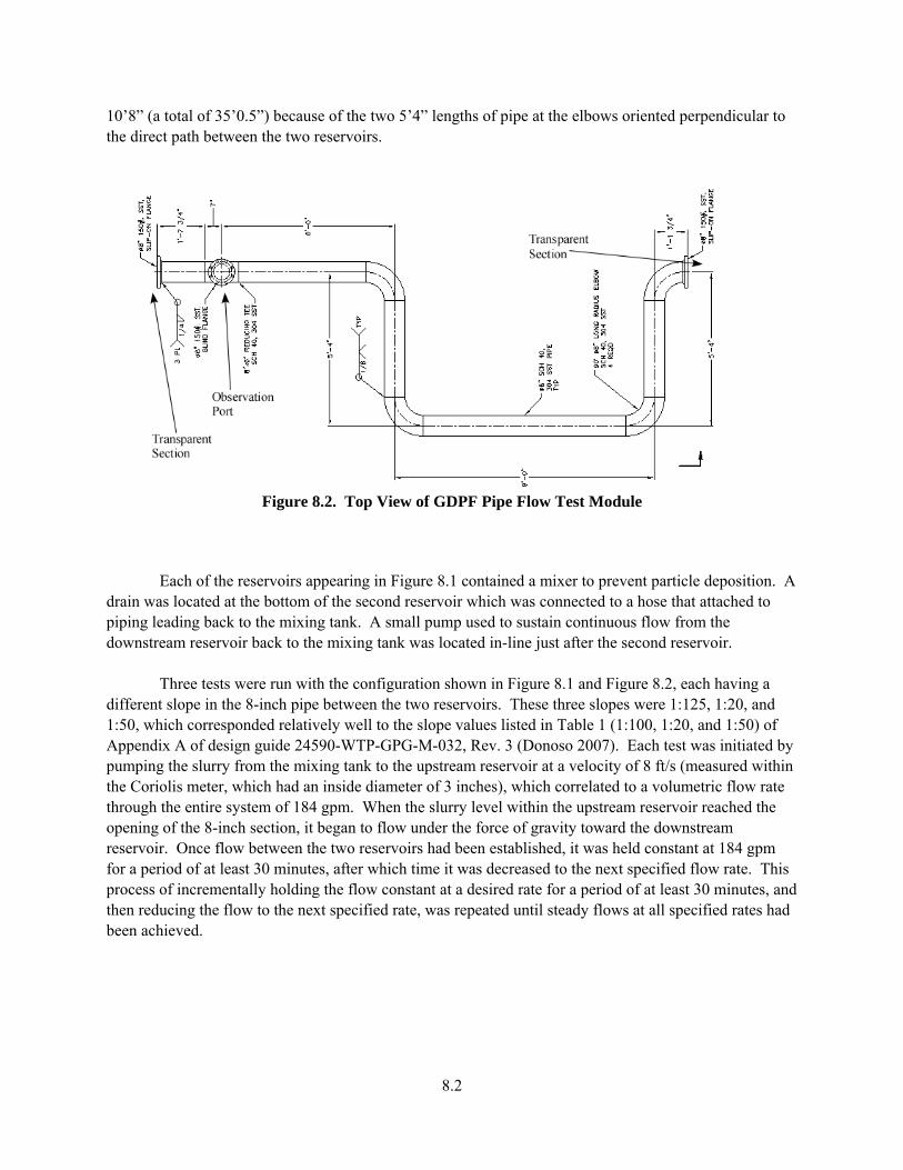
8.2
10’8” (a total of 35’0.5”) because of the two 5’4” lengths of pipe at the elbows oriented perpendicular to the direct path between the two reservoirs.
Figure 8.2. Top View of GDPF Pipe Flow Test Module
Each of the reservoirs appearing in Figure 8.1 contained a mixer to prevent particle deposition. A drain was located at the bottom of the second reservoir which was connected to a hose that attached to piping leading back to the mixing tank. A small pump used to sustain continuous flow from the downstream reservoir back to the mixing tank was located in-line just after the second reservoir. Three tests were run with the configuration shown in Figure 8.1 and Figure 8.2, each having a different slope in the 8-inch pipe between the two reservoirs. These three slopes were 1:125, 1:20, and 1:50, which corresponded relatively well to the slope values listed in Table 1 (1:100, 1:20, and 1:50) of Appendix A of design guide 24590-WTP-GPG-M-032, Rev. 3 (Donoso 2007). Each test was initiated by pumping the slurry from the mixing tank to the upstream reservoir at a velocity of 8 ft/s (measured within the Coriolis meter, which had an inside diameter of 3 inches), which correlated to a volumetric flow rate through the entire system of 184 gpm. When the slurry level within the upstream reservoir reached the opening of the 8-inch section, it began to flow under the force of gravity toward the downstream reservoir. Once flow between the two reservoirs had been established, it was held constant at 184 gpm for a period of at least 30 minutes, after which time it was decreased to the next specified flow rate. This process of incrementally holding the flow constant at a desired rate for a period of at least 30 minutes, and then reducing the flow to the next specified rate, was repeated until steady flows at all specified rates had been achieved.

8.3
8.2 Observation Methods
The gravity-driven partially-filled (GDPF) pipe flow tests did not include differential pressure transducer measurements, as did the other modular tests, because the slurry surface was open to the atmosphere. For this reason, system characterization by data analysis, as had been done for previous cases, was not possible. Instead, characterization of slurry behavior for the GDPF pipe flow tests was largely accomplished by visually monitoring the slurry flow through the transparent sections and through physical inspection of the slurry through the open ports, as well as inspecting the 8-inch pipe after the slurry pump had been stopped. Initially, qualitative observations were made about the slurry as it flowed through the transparent sections. Quantitative measurements were made during this initial testing period by holding a ruler up to each transparent section and directly measuring the solids deposition height. To better quantify such observations, a measuring tape was wrapped around each transparent section of the pipe. A picture of the upstream transparent section with this measuring tape in place is shown in Figure 8.3. Figure 8.4 is a close-up view of the measuring tape shown in Figure 8.3. It is a close enough view to show that the slurry height is measured at 5.75 inches on the measuring tape (the 5 cannot be seen in Figure 8.4 due to the presence of the reinforcement bar). Behavior of the slurry within the metal (non-transparent) sections of pipe, which included the four 90º elbows, had to be deduced from observations of slurry behavior in the transparent sections.

8.4
Figure 8.3. Side View of Upstream Transparent (Clear) Section with Measuring Tape
Figure 8.4. Close-up of Transparent (Clear) Section with Measuring Tape
Slurry Surface Slurry Surface
Slurry Surface Slurry Surface

8.5
The value taken from the measuring tape is a measure of the circumferential length from the top of the transparent section to the point of interest. For simplicity, this reading was converted into a vertical height from the bottom of the pipe correlating to a slurry height and a deposition height. Conversion from the measuring tape reading to deposition or slurry height follows from a geometric argument based on Figure 8.5.
Figure 8.5. Measurement Conversion Parameters
The measurement taken from the measuring tape will be equal to the arc-length “s” that appears in Figure 8.5. This length is related to the radius of the circular cross-section of the pipe by the equation Rs [8.1]
The value of h is then determined with the equation

8.6
2sinRh [8.2]
Equation [8.2] is valid even if the value of θ is greater than 2 . The result will simply be a negative
value for h. The value of H, which is equal to the height of the slurry or deposition layer, is then computed with the equation hRH [8.3] The inside diameter of the pipe used for the GDPF pipe flow tests was 7.981 inches. Standard observations at each flow rate were categorized according to several parameters indicated in Figure 8.6.
Figure 8.6. Common Observation Parameters in Transparent (Clear) Sections
8.3 Observations
During each test, observations were recorded in the Laboratory Record Book. Additionally, video recordings were made of slurry behavior in the transparent sections for each flow condition. For flow rates above 3.0 ft/s in the first test, the solid-deposition measurements were taken directly from a ruler held up to each transparent section. For the lower flow rates in the first test, and all flow rates in the second and third tests, measurements were taken with the measuring tape and converted as described in the previous section.
8.3.1 Test 1, Slope = 1:125 Test 1 had the shallowest slope and thus presented the greatest possibility for solids deposition and flow disruption. Table 8.1 lists the maximum deposition heights observed in the upstream and downstream transparent sections at each axial velocity tested. The observed values were recorded just prior to adjustment of the velocity, therefore maximum deposition had occurred for the test condition. The maximum deposition height tended to be at the downstream end of the upstream transparent section, but tended to fluctuate for the downstream section. The deposition length tended to increase for both
Upstream End
Fluid Height
Deposition Length
Downstream End
Maximum Deposition
Height

8.7
sections as the test progressed to lower velocities. Unfortunately, the deposition length and the axial position of the maximum deposition height were not quantitatively measured due to the continuously shifting shape of the solids deposition. Instead, sketches of the solids deposition patterns in each transparent section were made and recorded in a Laboratory Record Book. Duplications of these sketches are presented in Appendix B.
Table 8.1. Deposition Recorded in Test 1 (Slope = 1:125)
Volumetric Flow Rate (gpm)
Axial Velocity (through 3” Coriolis meter) (ft/s)
Upstream Clear Section Maximum Deposition Height “MDH” (inches)
Downstream Clear Section Maximum Deposition Height “MDH” (inches)
184 8.0 None Observed None Observed 173 7.5 None Observed None Observed 161 7.0 1* 1 150 6.5 1.5 1 138 6.0 2 1 126 5.5 2.5 1 115 5.0 3 1.5 103 4.5 3 1.5 93 4.0 3 1.5 80 3.5 2 1.2 68 3.0 2.3 1.1 58 2.5 2.8 1.1 45 2.0 2.8 1.1
*Italicized numbers were taken from measurements performed with a ruler. Non-italicized numbers were taken from measurements performed with a measuring tape.
The slurry-fluid height and shape during the tests changed more rapidly and dramatically than the solid-deposition height and shape. These slurry characteristics are included in the sketches mentioned above located in Appendix B. In addition to the sketches, still-frame clips were taken from video recordings of the transparent sections that were taken during testing to corroborate values included in the sketches. Selections from these clips showing slurry-fluid shape and height in each transparent section for each axial flow rate tested are included in Appendix A. The clips are listed in pairs, with a picture of the upstream transparent section placed just above a picture of the downstream section for each test condition. These pictures show that even at a velocity as high as 6 ft/s, slurry in the upstream transparent section became noticeably higher than slurry in the downstream transparent section. Some of this disparity between observations in the two transparent sections is due to more solids deposition in the upstream transparent section than in the downstream transparent section as documented in Table 8.1. The pictures do indicate, however, that the difference between slurry heights in the two transparent sections seems to become greater for lower flow rates. According to Table 8.1, however, the difference in solid-deposition heights in the two transparent sections does not seem to increase in the same pattern as the slurry height difference. This discrepancy is most likely due to solid deposition within the metal (non-transparent) portion of the pipe, where direct visual observation is not possible. Observations through the viewport located just downstream of the upstream transparent section indicated that the solid-deposition layers observed in the upstream transparent section continued down the pipe. It is likely that the solid-deposition layer may be higher near the elbows in the pipe. This would account for what appears in the pictures to be a gradual backup of slurry as the test progressed.

8.8
It is important to understand that the pictures in Appendix A are snapshots of the slurry height in each transparent section at specified times. The slurry did not flow smoothly, but would change shape and height erratically during a test. Thus, during a given test, it would be possible to obtain still frames that indicate that the difference in the slurry heights in the two transparent sections would be quite different than what is indicated by the pictures in the appendix. Effort was taken in the selection of the frames in this report to ensure that a good representation is given of average slurry behavior during a test condition. Figure 8.7 and Figure 8.8 show two views of the upstream transparent section after the conclusion of the test. Likewise, Figure 8.9 shows the downstream transparent section after conclusion of the test. The material seen in Figure 8.7 through Figure 8.9 is a combination of deposited solids and slurry that failed to drain from the pipe after the pump had stopped. Figure 8.10 through Figure 8.12 show the interiors of the upstream and downstream reservoirs, including the connections with the 8-inch pipe. These figures show that the slurry levels in the reservoirs were not influencing the post-test slurry levels or the solid-deposition levels shown in Figure 8.7 through Figure 8.9. In the test case with a slope of 1:125, deposition was seen at relatively high flow rates. As shown in Table 8.1 and Figure 8.7 through Figure 8.9, substantial quantities of solids settled during the test where 3-inch deposition height in an 8-inch pipe is defined as substantial solids deposition. These solid deposits were not easily removed from the piping after conclusion of the test. In an attempt to remove the deposits, the slurry was pumped through the pipe at a flow rate of 220 gpm. This did not successfully remove the deposits, which ultimately had to be removed with a pressurized water spray.

8.9
Figure 8.7. Upstream Post-Test Deposition
Figure 8.8. Upstream Post-Test Deposition
Deposited Solids Deposited Solids
Deposited Solids

8.10
Figure 8.9. Downstream Post-test Deposition
Figure 8.10. Pipe Entrance from Upstream Reservoir
Deposited Solids

8.11
Figure 8.11. Downstream Reservoir Post-Test
Figure 8.12. Pipe End to Reservoir Post-Test

8.12
8.3.2 Test 2, Slope = 1:20 Test 2 represented the design with the greatest slope and thus served as a bounding case to determine whether or not the GDPF pipe flow test arrangement would function within the scope of the current tests. In this case, no solids deposition was observed in either transparent section at any flow rate under normal operating conditions. However, a pump malfunction during the test caused the slurry to remain stationary within the pipe for a period of time, which resulted in some solids buildup. After fixing the pump and restarting the test, no deposition was observed at any flow rate under normal operating conditions. As no solid deposition was directly observed in this test case, observations of the slurry height in each transparent section were recorded. As mentioned in the description of the previous test, the slurry behavior was quite erratic. However, the slurry height was observed over a period of time and the height that most accurately represented the average slurry height was recorded. The observed slurry heights for both transparent sections are recorded in Table 8.2. Contrary to the results from Test 1, the slurry height was greater in the downstream transparent section than in the upstream transparent section for nearly every condition in Test 2. This was largely an effect of the greater slope and did not provide evidence of solid deposition within the elbows of the pipe until the last test condition of 1.5 ft/s. The decrease in slurry height in the downstream transparent section, and the rise in the upstream transparent section slurry height between the last two test conditions, may be indicative of some solid deposition within the elbows. To supplement the values in Table 8.2, as with the previous test, pictures of the slurry behavior in both transparent sections for each test condition are located in Appendix A. Fewer test cases were run for this slope (only integer-value velocities were studied, except for the final test condition of 1.5 ft/s). For some test cases, a regular view and a close-up view of the same transparent section are provided. The close-up views allow the slurry heights to be correlated to values on the measuring tape. Unfortunately, one of the braces used to secure the downstream transparent section obscured the view of the top of the slurry for velocities above 2.0 ft/s. One must be careful not to confuse the brace seen on the back side of the transparent section with the slurry.
Table 8.2. Slurry Heights Recorded in Test 2 (Slope = 1:20)
Volumetric Flow Rate (gpm)
Axial Velocity (through
3” Coriolis meter) (ft/s) Upstream Slurry Height (inches)
Downstream Slurry Height (inches)
184 8.0 2.3 3.3 161 7.0 2.3 3.3 138 6.0 1.9 2.8 115 5.0 1.9 2.3 93 4.0 1.5 2.1 68 3.0 1.3 1.9 45 2.0 0.9* 1.3 33 1.5 1.8 0.9 *The upstream slurry height of 0.9 was the minimum height observed in this configuration. This behavior is analogous to a J-curve for determining critical velocities and indicates that deposition began to occur between the two transparent sections at this flow rate.
Figure 8.13 and Figure 8.14 are pictures of the post-test solid deposition in the upstream and downstream transparent sections, respectively. These figures confirm that very little solid deposition

8.13
occurred during the test. However, during the course of Test 2, the pump located downstream of the second reservoir tank broke down and the test had to be postponed. While the system was being reconfigured to transfer slurry from the reservoirs back to the mixing tank, solids were observed to deposit within the tube. After the pump was replaced, Test 2 was completed. Prior to the pump failure, the test condition of 3 ft/s had been completed, so the final two test conditions of 2 ft/s and 1.5 ft/s were run after the pump had been replaced. Figure 8.13 and Figure 8.14 are pictures taken after the conclusion of the 1.5 ft/s test condition. The material that can be seen in the two pictures is not from solids deposition during the test. Instead, it is slurry that did not drain from the pipe after the slurry pump was shut down. When the pump stopped, the slurry in the pipe continued to flow to the downstream reservoir and the slurry above the entrance level of the 8-inch pipe in the upstream reservoir continued to flow into the pipe. The material that appears in Figure 8.13 and Figure 8.14 is the slurry that remained after the slurry level in the upstream reservoir dropped to the pipe entrance level and the slurry in the pipe stopped flowing into the downstream reservoir. The perspectives shown in the two figures are not the same, making direct comparisons between them difficult. However, there does appear to be more material in the upstream transparent section than in the downstream transparent section. This disparity in the slurry heights in the two transparent sections may be an indication of a gradual increase in remaining material from the downstream to the upstream section of the pipe.
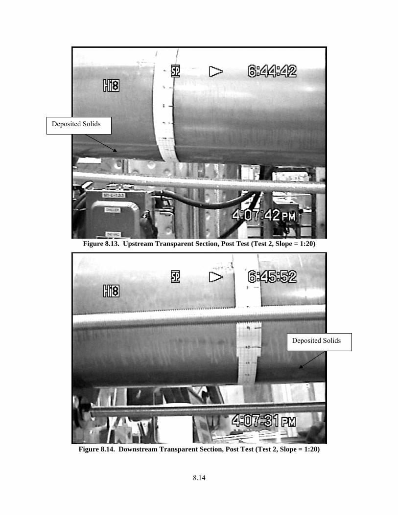
8.14
Figure 8.13. Upstream Transparent Section, Post Test (Test 2, Slope = 1:20)
Figure 8.14. Downstream Transparent Section, Post Test (Test 2, Slope = 1:20)
Deposited Solids
Deposited Solids

8.15
8.3.3 Test 3, Slope = 1:50 Test 3 represented a design with an intermediate slope and thus was used to determine a graded relation between the first and second tests. Observations made during Test 3 are recorded in Table 8.3 and Table 8.4. Particle deposition was observed in both transparent sections; however, the deposition occurred at higher flow rates and in greater quantities in the upstream transparent section than in the downstream transparent section. As in Test 1, the slurry height differences between the two transparent test sections for the final three test conditions is likely a result of solid deposition within the elbows of the pipe.
Table 8.3. Observed Upstream Parameters (Test 3, Slope = 1:50)
Volumetric Flow Rate (gpm)
Axial Velocity (through 3” Coriolis meter) (ft/s)
Maximum Deposition Height “MDH” (inches)
Deposition Length (inches)
Slurry Height (inches)
184 8.0 0 0 2.8 161 7.0 0 0 2.5 138 6.0 0 0 2.3 115 5.0 Trace 14 3.0 93 4.0 0.1 16 3.0 68 3.0 0.6 22 3.0 45 2.0 0.8 22 3.0 33 1.0 1.5 22 2.8
Table 8.4. Observed Downstream Parameters (Test 3, Slope = 1:50)
Volumetric Flow Rate (gpm)
Axial Velocity (through 3” Coriolis meter) (ft/s)
Maximum Deposition Height “MDH” (inches)
Deposition Length (inches)
Slurry Height (inches)
184 8.0 0 0 2.8 161 7.0 0 0 2.5 138 6.0 0 0 2.3 115 5.0 0 0 2.1 93 4.0 0 0 1.9 68 3.0 0 0 1.5 45 2.0 Trace 1 1.1 33 1.0 0.3 15 1.1 As with the first two tests, still frames from video recordings from both transparent sections at each test condition are located in Appendix A. Figure 8.15 through Figure 8.17 are post-test pictures of the transparent sections. As with the post-test pictures of the other two tests, the material seen in Figure 8.15 through Figure 8.17 is a combination of solid deposits and slurry that did not drain after the pump stopped.

8.16
Figure 8.15. Upstream, Slope = 1:50, Post-Test Deposition
Figure 8.16. Downstream, Slope = 1:50, Post-Test Deposition
Deposited Solids

8.17
Figure 8.17. Downstream, Slope = 1:50, Post-Test Deposition (Close-up)
8.4 Discussion
The results of the GDPF pipe flow tests cannot be directly compared to design guides 24590-WTP-GPG-M-027, Rev. 5 (Kloster 2007) and 24590-WTP-GPG-M-032, Re. 3 (Donoso 2007) because the tests used a Bingham-plastic slurry and the design guides only address Newtonian fluids and slurries. However, the test results do give some indication of how to design vessel-overflow lines for systems using slurries with yield stresses and viscosities similar to those of the slurry used in the tests. The results are limited in that they do not encompass the full transient nature of any specific overflow conditions. For instance, if the vessel overflow was not steady, but consisted of several “pulses” of slurry flowing at a low flow rate, then it can be expected that more settling would occur than is indicated by the results of this test. This statement is exemplified by the fact that in the test with a pipe slope of 1:20, no solid deposition was seen during normal operation at specified test conditions, but deposition did occur when the slurry was allowed to stand within the pipe for brief periods after the pump malfunction and after conclusion of the test.
The GDPF pipe flow test results suggest that a slope of 1:125 may not be suitable for the slurry type
and test conditions used in these tests. For this test condition, solid deposition was observed for flow velocities as high as 7.0 ft/s. Much larger deposition quantities were observed at lower velocities. Additionally, after the completion of the test, these deposits were very difficult to remove from inside the pipe. Although no line plugging was observed over the course of the test, significant deposition of solid
Deposited Solids

8.18
material was observed. It is possible that given longer term build-up, line plugging may become a problem. The shallowest slope discussed in design guide 24590-WTP-GPG-M-032, Re. 3 (Donoso 2007) is 1:100, for which it is suggested that a Newtonian slurry with a viscosity/specific gravity ratio of less than 41 centistokes would properly drain. Although the viscosity/specific gravity ratio of the slurry used in this test was well below this value, it was non-Newtonian and the slope of the pipe was less than 1:100.
Although significant solid deposition did not occur until lower flow velocities in the case of the 1:50
slope relative to the 1:125 slope, the test results indicate that the 1:50 slope may also be inadequate for the conditions considered. Any flow velocity less than 5.0 ft/s can be expected to result in some solid deposition. As was the case in the system with the 1:125 slope, the solid deposition was difficult to remove from the pipe upon conclusion of the test. Once again, although solid deposition was observed, plugging did not occur during the test, and it is difficult to tell what may have happened had the test been run at lower flow rates for a longer period of time.
The system with a 1:20 slope appeared to be adequate for overflow removal for most of the test
conditions considered. Although no solid deposition was observed during normal test conditions, slurry height measurements indicate that deposition may be occurring within the elbows for flow velocities at or below 1.5 ft/s. Additionally, stagnant conditions that occurred at the conclusion of the test resulted in some solid deposition.
Of the three test conditions studied in the GDPF pipe flow tests, only the system with the greatest
slope appeared to function as desired during normal test conditions. Even that system, with a slope of 1:20, showed indications of possible deposition at low flow velocities. In each case, stagnant conditions resulted in the formation of solid deposition layers within the pipe, and in each case, these deposits were difficult to flush from the pipe. Even after the pipe had been thoroughly flushed at the end of each test, when the system was disassembled for reconfiguration, it was discovered that deposits remained within the pipe. It is apparent that for any system used, it will be necessary to thoroughly flush out the overflow channel after a vessel-overflow event has occurred.

9.1
9.0 Flush-System Test Design guide 24590-WTP-GPG-M-0058, Rev. 0 (Hall 2006) specifies upper limits on the flushing
velocity of 12 ft/sec and 10 ft/sec for the process streams with and without the glass-former chemicals, respectively. This upper limit is in place to limit pipe erosion. The flush-volume upper limit is stated as 3 line volumes. The lower flush-volume limits are 1.5 and 1.7 line volumes for Newtonian and non-Newtonian process lines, respectively. The experimental flow loop under each test configuration setup was determined to have approximately 65 gallons of line volume. This section discusses how the prototypic flush performed with respect to the constraints of design guide 24590-WTP-GPG-M-058, Rev. 0 (Hall 2006) for the flow-loop test system with modular test sections of the gravity-feed and process-drain test module, the jumper test module, the complex-geometry test module, and the reducer and vertical-rise test module.
During each test the flush tank (pressure vessel) would be filled with an initial charge of water. Once a set of tests was done under any given configuration, valves were reconfigured to operate in flush mode. This mode allowed for flow from the flush tank to go to the spent-simulant vessel. The pressure in the tank was then increased to a target value, nominally 100 to 110 psig. A valve was opened, and the high-pressure water flush removed deposited slurry particles from the pipe loop.
9.1 Test Results
Following the procedure presented in Subsection 6.1, a high-pressure flush was conducted after the pressure-drop measurements. The initial charge pressure for line flushes was set between 100 and 110 psig. The flush system was opened, and the data acquisition system recorded pressures, flow rates, and slurry density.
The level in the flush tank was recorded and converted to a volume using a calibration curve. The ratio of the cumulative flush tank volume discharge to the 65-gallon loop volume is used as the flush-to-line-volume ratio.
The reported pressure is the flow-loop pressure drop described in Section 5. The reported velocities are from the loop-entrance Coriolis flow meter. If the settled solids in the system form a stationary plug of material, water should flow through that plug slowly, providing a near-zero velocity reading on the system flow meters while the flush-tank level drops.
The reported density is taken from the outlet Coriolis flow meter. When the measured density is high, the flush is still removing particles from the system. As density approaches the value of the flush water, the effectiveness of the flush is nearing completion.
A target flush volume of 1.5 to 2 line volumes was selected, and multiple flushes were performed. This resulted in a total flush-to-line-volume ratio typically between 5 and 6. After this point, the system was purged with compressed air. This is reflected by the abrupt drop in instrumentation signal at the end of several of the plots. Data from the flush testing is shown in Figure 9.1 to Figure 9.5 for each modular test configuration. The flush operation was conducted in the last test run for each modular test configuration.

9.2
Figure 9.1 and Figure 9.2 belong to the same test flush set as the gravity-feed and process-drain test module. Here, the disk ruptured during the first flush, resulting in replacement of the disk. The disk rupture occurred due to a pressure surge (wave) produced by manually opening the valve rapidly. After the disk replacement, the remaining flushes were continued as shown in Figure 9.2. Figure 9.3, Figure 9.4 and Figure 9.5 show the flush plots for the jumper test module, the complex-geometry test module, and the reducer and vertical-rise test module, respectively.
0
10
20
30
40
50
60
0 0.5 1 1.5 2 2.5 3
Flush to Loop Volume Ratio
Pre
ssu
re [
psi
g]
an
d V
elo
city
[ft
/s]
0
0.2
0.4
0.6
0.8
1
1.2
1.4
1.6
1.8
Den
sity
[g
/mL
]
Pressure
Velocity
Density
Figure 9.1. Flush Data for the gravity-feed and process-drain test module as a flush-to-pipe loop-volume
ratio, showing the flush before disk rupture

9.3
0
5
10
15
20
25
30
35
0 1 2 3 4 5 6 7
Tank to Loop Volume ratio
Pre
ss
ure
[p
sig
] a
nd
Ve
loc
ity
[ft
/s]
-0.2
0
0.2
0.4
0.6
0.8
1
1.2
De
nsi
ty [
g/m
L]
Density
Pressure
Velocity
Figure 9.2. Flush data for the gravity-feed and process-drain test module as a flush-to-pipe loop-volume
ratio, showing two complete flushes after disk replacement (continuation of Figure 9.1)
0
10
20
30
40
50
60
70
0 1 2 3 4 5 6 7
Tank to Loop Volume Ratio
Pre
ss
ure
[p
sig
] a
nd
Ve
loc
ity
[ft
/s]
-0.5
0
0.5
1
1.5
2
Den
sity
[g
/mL
]
Pressure
Velocity
Density
Figure 9.3. Flush data for the jumper test module as a flush-to-pipe loop-volume ratio, showing three
complete flushes

9.4
0
10
20
30
40
50
60
70
80
0 1 2 3 4 5 6 7
Tank to Loop Volume Ratio
Pre
ssu
re [
ps
ig]
and
Vel
oci
ty [
ft/s
ec]
-0.2
0
0.2
0.4
0.6
0.8
1
1.2
1.4
1.6
1.8
2
Des
nit
y [g
/mL
]
PressureVelocity
Density
Figure 9.4. Flush data for the complex-geometry test module as a flush-to-pipe loop-volume ratio,
showing four complete flushes
0
10
20
30
40
50
60
70
0 1 2 3 4 5 6 7
Tank to Loop Volume Ratio
Pre
ssu
re [
psi
g]
and
Vel
oci
ty [
ft/s
ec]
-0.2
0
0.2
0.4
0.6
0.8
1
1.2
1.4
1.6
Den
sity
[g
/mL
]
Pressure
Velocity
Density
Figure 9.5. Flush data for the reducer and vertical-rise test module as a flush-to-pipe loop-volume ratio,
showing four complete flushes

9.5
9.2 Discussion
The flushing operations for this testing were performed by employing the recommendation provided by Poloski et al. (2008) as: “The pneumatic flush system must be opened slowly to erode the sediment bed from the top down. If the pneumatic flush system is opened quickly, the sediment bed is simply pushed to the nearest corner, and a granular plug develops and completely fills the line cross-sectional area.”
From Figure 9.1 to Figure 9.5, the following observations are made:
o The flush system is effective in removing sediment beds from the flow-loop system
o The total flush-to-line-volume ratio is approximately 6
o For all of the test modules, except the gravity-feed and process-drain test module, the minimum flush-to-line volume ratio of 1.7 (for non-Newtonian fluids) appears to be satisfied
o The flush-to-line volume ratio for the flow-loop system with the gravity-feed and process-drain test module is approximately 2.9
o For all of the test modules, a flush-to-line volume ratio of 3 appears to be sufficient to remove the particles from the flow-loop system
o For all of the test modules, except the gravity-feed and process-drain test module, the highest flushing velocities are nearly 20 ft/sec
o The highest flushing velocity for the flow-loop system with the gravity-feed and process-drain test module is nearly 30 ft/sec
For the flow-loop system with the gravity-feed and process-drain test module, the solid settlement
was expected within the “tee” fitting. In addition, the solids were considered to be trapped within all of the 90o 3D elbows. Therefore, it is deemed that these factors caused the higher flush-to-line volume ratio for the flow-loop system with the gravity-feed and process-drain test module.
The values of the flush volume and the flush velocity specified by design guide 24590-WTP-GPG-M-
0058, Rev. 0 (Hall 2006) were difficult to be satisfied manually. Depending on the process-line geometry, flows in the range of 500 to 1,000 gpm can be achieved with this system. Since the piping volumes may be on the order of 50 to 100 gallons, manually closing a valve to hit this target volume may be challenging. Compounding this problem, the valves need to be closed slowly to avoid water hammer.

10.1
10.0 Findings The following findings are obtained from the test results provided in this report:
A complete flow blockage by pipe plugging did not occur at the smallest flow velocity used for the testing; however, the flow velocity was kept constant by the feedback system of the pump with the variable frequency drive (VFD)
Due to high uncertainty in the critical velocity evaluations in the absence of a definite J-curve profile, velocities for avoiding deposition (VFAD) provide velocities at which it is assured that no particle deposition occur
A definite profile of the J-curve was not obtained in this testing due to high fluctuations in DPT data
Smallest velocities obtained in this testing need not to be critical velocities
The critical velocities were evaluated from the uncorrected DPT data by applying the critical velocity definition used by Poloski et al. (2008) and it was found that, except in the case of a tee in the gravity-feed and process-drain test spool, the evaluated critical velocities for the fittings used for in this testing are lower than that for a straight horizontal pipe reported by Poloski et al. (2008) where the same pipe diameter of 3 inches as that used in this testing and the slurry composition and rheology similar to those used in this testing were used; however, high uncertainty in the critical velocity evaluations is expected
In the overflow-relief piping test, for the minimum flow rate of 45 gpm for the 1:125 slope, and the minimum flow rate of 33 gpm for the 1:50 and 1:20 slopes, a complete flow blockage by pipe plugging did not occur and the following observations are reported:
o At the slope of 1:125, 1) substantial solids deposition occurred at a flow rate of 161 gpm and below, where 3-inch deposition height in an 8-inch pipe is defined as substantial solids deposition, and 2) it is conceivable that a complete flow blockage is possible under certain conditions
o At the slope of 1:50, 1) substantial solids deposition occurred at a flow rate of 93 gpm and below and 2) small amounts of solids deposition occurred at the flow rate of 115 gpm
o At the slope of 1:20, no deposition occurred at any of the flow rates used in the testing
o For all three slopes, removing the deposited particles from the pipe surface was difficult; therefore, it is recommended to assure that the overflow channel system is thoroughly flushed out after a vessel-overflow event
From the flush tests, it was found that a flush-to-line volume ratio of 3 was needed to remove sediment beds from the flow-loop system with the gravity-feed and process-drain test spool whereas design-guide 24590-WTP-GPG-M-0058, Rev. 0 (Hall 2006) provides a minimum flush-volume ratio of 1.7 for non-Newtonian fluids. The design-guide appears to be satisfied for the jumper test spool, the complex-geometry test spool, and the reducer and vertical-rise test spool. For all of the test spools, the flushing operations were performed with the following caveats:
o The pneumatic flush system must be opened slowly to erode the sediment bed from the top down. If the pneumatic flush system is opened quickly, the sediment bed is simply pushed to the nearest corner, and a granular plug develops and completely fills the line cross-sectional area.

10.2
o The design guide values for flush volume and flush velocity were difficult to achieve manually. Depending on the process-line geometry, flows in the range of 500 to 1,000 gpm can be achieved with this system. Since the piping volumes may be on the order of 50 to 100 gallons, manually closing a valve to hit this target volume may be challenging. Compounding this problem, valves need to be closed slowly to avoid water hammer.
A definite profile of the J-curve was not obtained in this testing due to high uncertainty in the DPT data. The following are considered sources of the uncertainty:
o The uncorrected DPT data include the hydrostatic pressure due to gravity that varies over a test run since the density changes as the flow velocity changes. The density change is considered to be significant in the lower-velocity region, possibly due to the slurry-particle deposition.
o Complex slurry flow is expected in the immediate vicinity of the pressure ports produced by the geometry of the modular component and considered to cause the high fluctuations in DPT data.
o High uncertainty in the corrected DPT data is expected since the slurry density was measured at a position well upstream of the modular test section and considered to be different, especially in low velocity conditions, from the density at the pressure ports. In addition, the expected complex slurry flow structure produced by the geometry of the modular component might cause density variations.

11.1
11.0 References 10 CFR 830. “Nuclear Safety Management.” Code of Federal Regulations, U.S. Department of Energy. Bechtel National, Inc. (BNI). 2007. Evaluation of Waste Slurry Critical Velocity and Line Flush Capabilities in WTP Process Piping. 24590-WTP-TSP-RT-07-005, Rev. 0, BNI, Richland, Washington. DOE Order 414.1C. 2005. “Quality Assurance.” U.S. Department of Energy, Washington, D.C. Donoso ED. 2007. Vessel Overflow and Gravity Line Sizing. WTP Project Doc. No. 24590-WTP-GPG-M-032, Rev. 3, Bechtel National, Inc., Richland, Washington. Hall MN. 2006. Minimum Flow Velocity for Slurry Lines. WTP Project Doc. No. 24590-WTP-GPG-M-0058, Rev. 0, Bechtel National, Inc., Richland, Washington. Hall MN. 2007. Pipe Sizing for Lines with Liquids Containing Solids—Bingham Plastic Model. WTP Project Doc. No. 24590-WTP-GPG-M-016, Rev. 2, Bechtel National, Inc., Richland, Washington. Kloster G. 2007. Recommended Slopes for Piping Systems. WTP Project Doc. No. 24590-WTP-GPG-M-027, Rev. 5, Bechtel National, Inc., Richland, Washington. Poloski AP. 2007. M1/M6 Flow Loop Testing with Prototypic WTP Test Modules. TP-RPP-WTP-494, Rev. 0, Pacific Northwest National Laboratory, Richland, Washington. Poloski AP, HE Adkins, J Abrefah, AM Casella, RE Hohimer, F Nigl, MJ Minette, JJ Toth, JM Tingey, and ST Yokuda. 2008. Deposition Velocities of Newtonian and Non-Newtonian Slurries in Pipelines. WTP-RPT-175, Rev. 0 (PNNL-17638), Pacific Northwest National Laboratory, Richland, Washington. Smith GL, and K Prindiville. 2002. Guidelines for Performing Chemical, Physical, and Rheological Properties Measurements. 24590-WTP-GPG-RTD-001 Rev 0, Bechtel National, Inc., Richland, WA.

A.1
Appendix A: Gravity-Driven Partially-Filled Pipe Flow Test Condition Pictures
Each picture in this Appendix is identified by location, slope, and velocity. The location is either
“Upstream”, referring to the upstream transparent section or “Downstream”, referring to the downstream transparent section. The slope is either “1:125” which indicates that the picture comes from the first test,
“1:20” which indicates that the picture comes from the second test, or “1:50” which indicates that the picture comes from the third test. The listed velocity indicates the velocity at which the slurry was
flowing through the pipe when the picture was taken.

A.2
Figure A.1. Upstream, Slope = 1:125, Velocity = 8 ft/s
Figure A.2. Downstream, Slope = 1:125, Velocity = 8 ft/s
Slurry Surface
Slurry Surface
Slurry Surface
Slurry Surface

A.3
Figure A.3. Upstream, Slope = 1:125, Velocity = 7.5 ft/s
Figure A.4. Downstream, Slope = 1:125, Velocity = 7.5 ft/s
Slurry Surface
Slurry Surface
Slurry Surface
Slurry Surface

A.4
Figure A.5. Upstream, Slope = 1:125, Velocity = 7.0 ft/s
Figure A.6. Downstream, Slope = 1:125, Velocity = 7.0 ft/s
Slurry Surface
Slurry Surface
Slurry Surface
Slurry Surface

A.5
Figure A.7. Upstream, Slope = 1:125, Velocity = 6.5 ft/s
Figure A.8. Downstream, Slope = 1:125, Velocity = 6.5 ft/s
Slurry Surface
Slurry Surface
Slurry Surface
Slurry Surface
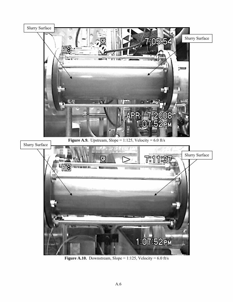
A.6
Figure A.9. Upstream, Slope = 1:125, Velocity = 6.0 ft/s
Figure A.10. Downstream, Slope = 1:125, Velocity = 6.0 ft/s
Slurry Surface
Slurry Surface
Slurry Surface
Slurry Surface
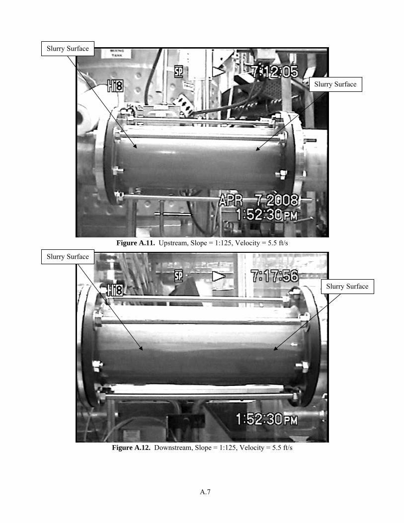
A.7
Figure A.11. Upstream, Slope = 1:125, Velocity = 5.5 ft/s
Figure A.12. Downstream, Slope = 1:125, Velocity = 5.5 ft/s
Slurry Surface
Slurry Surface
Slurry Surface
Slurry Surface

A.8
Figure A.13. Upstream, Slope = 1:125, Velocity = 5.0 ft/s
Figure A.14. Downstream, Slope = 1:125, Velocity = 5.0 ft/s
Slurry Surface
Slurry Surface
Slurry Surface
Slurry Surface

A.9
Figure A.15. Upstream, Slope = 1:125, Velocity = 4.5 ft/s
Figure A.16. Downstream, Slope = 1:125, Velocity = 4.5 ft/s
Slurry Surface
Slurry Surface
Slurry Surface
Slurry Surface

A.10
Figure A.17. Upstream, Slope = 1:125, Velocity = 4.0 ft/s
Figure A.18. Downstream, Slope = 1:125, Velocity = 4.0 ft/s
Slurry Surface
Slurry Surface
Slurry Surface
Slurry Surface

A.11
Figure A.19. Upstream, Slope = 1:125, Velocity = 3.5 ft/s
Figure A.20. Downstream, Slope = 1:125, Velocity = 3.5 ft/s
Slurry Surface Slurry Surface
Slurry Surface
Slurry Surface

A.12
Figure A.21. Upstream, Slope = 1:125, Velocity = 3.0 ft/s
Figure A.22. Downstream, Slope = 1:125, Velocity = 3.0 ft/s
Slurry Surface
Slurry Surface
Slurry Surface
Slurry Surface
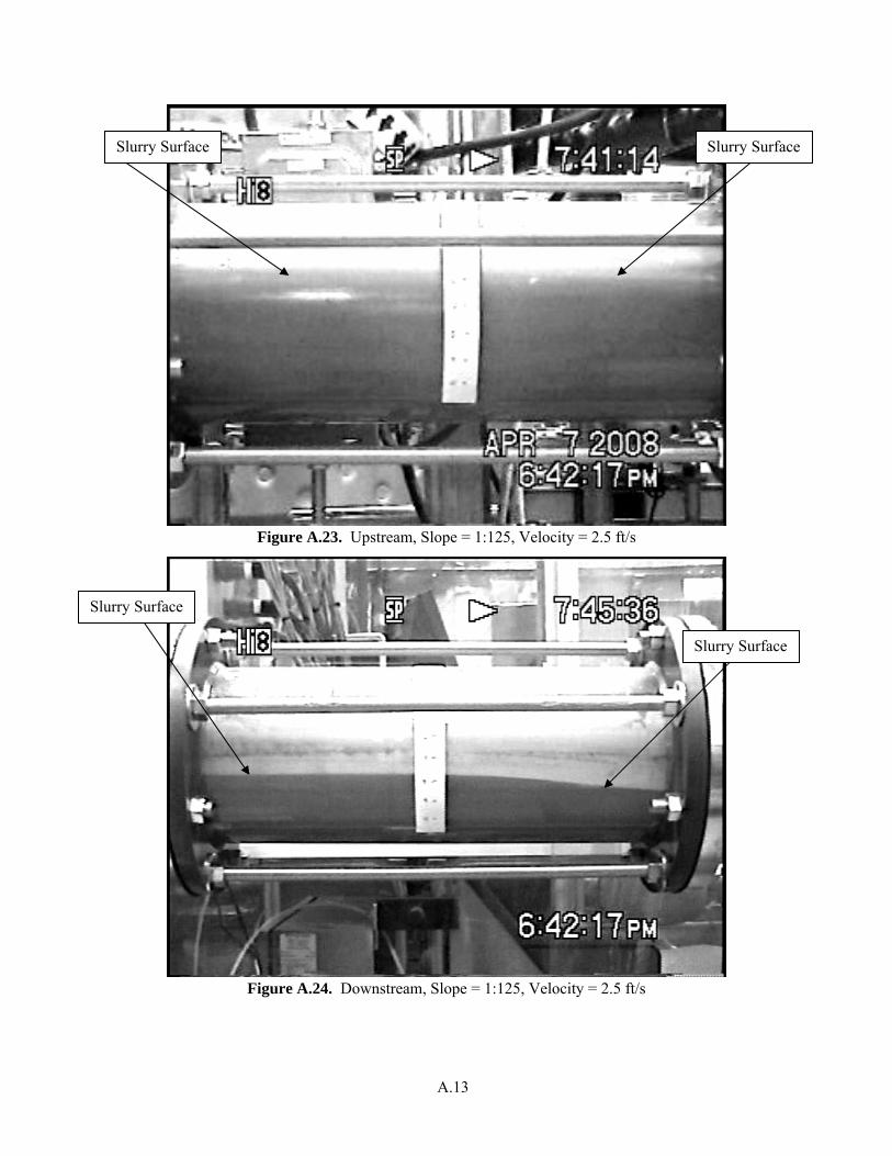
A.13
Figure A.23. Upstream, Slope = 1:125, Velocity = 2.5 ft/s
Figure A.24. Downstream, Slope = 1:125, Velocity = 2.5 ft/s
Slurry Surface
Slurry Surface
Slurry Surface
Slurry Surface

A.14
Figure A.25. Upstream, Slope = 1:125, Velocity = 2.0 ft/s
Figure A.26. Downstream, Slope = 1:125, Velocity = 2.0 ft/s
Slurry Surface
Slurry Surface
Slurry Surface
Slurry Surface

A.15
Figure A.27. Upstream, Slope = 1:20, Velocity = 8.0 ft/s
Figure A.28. Downstream, Slope = 1:20, Velocity = 8.0 ft/s
Slurry Surface
Slurry Surface
Slurry Surface Slurry Surface

A.16
Figure A.29. Upstream, Slope = 1:20, Velocity = 8.0 ft/s
Figure A.30. Downstream, Slope = 1:20, Velocity = 8.0 ft/s
Slurry Surface
Slurry Surface
Slurry Surface
Slurry Surface

A.17
Figure A.31. Upstream, Slope = 1:20, Velocity = 7.0 ft/s
Figure A.32. Downstream, Slope = 1:20, Velocity = 7.0 ft/s
Slurry Surface
Slurry Surface
Slurry Surface
Slurry Surface

A.18
Figure A.33. Upstream, Slope = 1:20, Velocity = 6.0 ft/s
Figure A.34. Downstream, Slope = 1:20, Velocity = 6.0 ft/s
Slurry Surface
Slurry Surface
Slurry Surface
Slurry Surface

A.19
Figure A.35. Upstream, Slope = 1:20, Velocity = 5.0 ft/s
Figure A.36. Downstream, Slope = 1:20, Velocity = 5.0 ft/s
Slurry Surface
Slurry Surface
Slurry Surface
Slurry Surface

A.20
Figure A.37. Upstream, Slope = 1:20, Velocity = 4.0 ft/s
Figure A.38. Downstream, Slope = 1:20, Velocity = 4.0 ft/s
Slurry Surface
Slurry Surface
Slurry Surface
Slurry Surface

A.21
Figure A.39. Upstream, Slope = 1:20, Velocity = 3.0 ft/s –pump broke soon after
Figure A.40. Downstream, Slope = 1:20, Velocity = 3.0ft/s
Slurry Surface
Slurry Surface
Slurry Surface
Slurry Surface

A.22
Figure A.41. Upstream, Slope = 1:20, Velocity = 2.0 ft/s
Figure A.42. Downstream, Slope = 1:20, Velocity = 2.0 ft/s
Slurry Surface
Slurry Surface
Slurry Surface
Slurry Surface
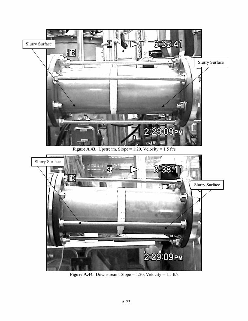
A.23
Figure A.43. Upstream, Slope = 1:20, Velocity = 1.5 ft/s
Figure A.44. Downstream, Slope = 1:20, Velocity = 1.5 ft/s
Slurry Surface
Slurry Surface
Slurry Surface
Slurry Surface

A.24
Figure A.45. Upstream, Slope = 1:50, Velocity = 8.0 ft/s
Figure A.46. Downstream, Slope = 1:50, Velocity = 8.0 ft/s
Slurry Surface
Slurry Surface
Slurry Surface
Slurry Surface

A.25
Figure A.47. Upstream, Slope = 1:50, Velocity = 7.0 ft/s
Figure A.48. Downstream, Slope = 1:50, Velocity = 7.0 ft/s
Slurry Surface
Slurry Surface
Slurry Surface
Slurry Surface

A.26
Figure A.49. Upstream, Slope = 1:50, Velocity = 6.0 ft/s
Figure A.50. Downstream, Slope = 1:50, Velocity = 6.0 ft/s
Slurry Surface
Slurry Surface
Slurry Surface
Slurry Surface

A.27
Figure A.51. Upstream, Slope = 1:50, Velocity = 5.0 ft/s
Figure A.52. Downstream, Slope = 1:50, Velocity = 5.0 ft/s
Slurry Surface
Slurry Surface
Slurry Surface Slurry Surface
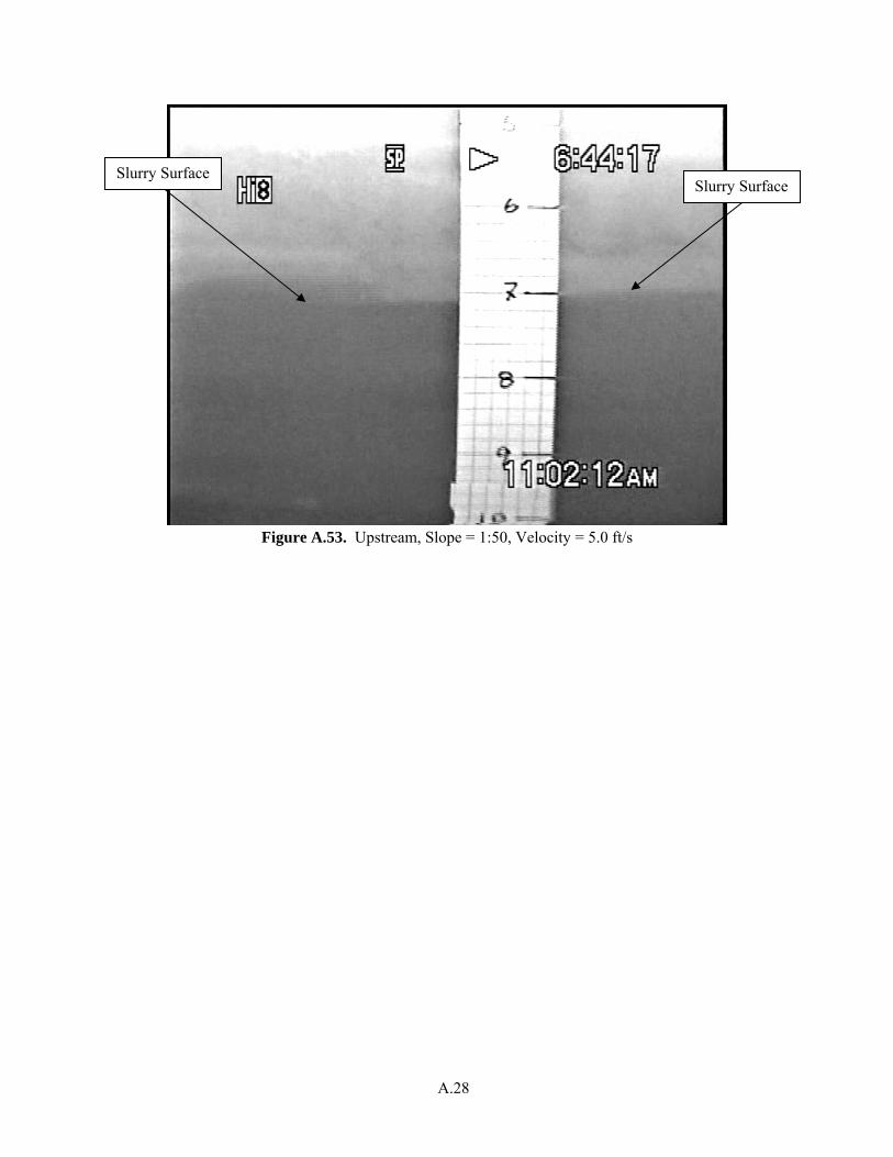
A.28
Figure A.53. Upstream, Slope = 1:50, Velocity = 5.0 ft/s
Slurry Surface Slurry Surface

A.29
Figure A.54. Upstream, Slope = 1:50, Velocity = 4.0 ft/s
Figure A.55. Downstream, Slope = 1:50, Velocity = 4.0 ft/s
Slurry Surface
Slurry Surface
Slurry Surface
Slurry Surface

A.30
Figure A.56. Upstream, Slope = 1:50, Velocity = 4.0 ft/s
Figure A.57. Downstream, Slope = 1:50, Velocity = 4.0 ft/s
Slurry Surface Slurry Surface
Slurry Surface
Slurry Surface

A.31
Figure A.58. Upstream, Slope = 1:50, Velocity = 3.0 ft/s
Figure A.59. Downstream, Slope = 1:50, Velocity = 3.0 ft/s
Slurry Surface
Slurry Surface
Slurry Surface
Slurry Surface

A.32
Figure A.60. Upstream, Slope = 1:50, Velocity = 3.0 ft/s
Figure A.61. Downstream, Slope = 1:50, Velocity = 3.0 ft/s
Slurry Surface
Slurry Surface
Slurry Surface Slurry Surface

A.33
Figure A.62. Upstream, Slope = 1:50, Velocity = 2.0 ft/s
Figure A.63. Downstream, Slope = 1:50, Velocity = 2.0 ft/s
Slurry Surface
Slurry Surface
Slurry Surface
Slurry Surface

A.34
Figure A.64. Upstream, Slope = 1:50, Velocity = 1.0 ft/s
Figure A.65. Downstream, Slope = 1:50, Velocity = 1.0 ft/s
Slurry Surface
Slurry Surface
Slurry Surface
Slurry Surface

A.35
Figure A.66. Upstream, Slope = 1:50, Velocity = 1.0 ft/s
Figure A.67. Downstream, Slope = 1:50, Velocity = 1.0 ft/s
Slurry Surface
Slurry Surface
Slurry Surface
Slurry Surface

B.1
Appendix B: Sketches of Slurry in Transparent Sections During Gravity-Driven Partially-Filled Pipe Flow Test
Conditions
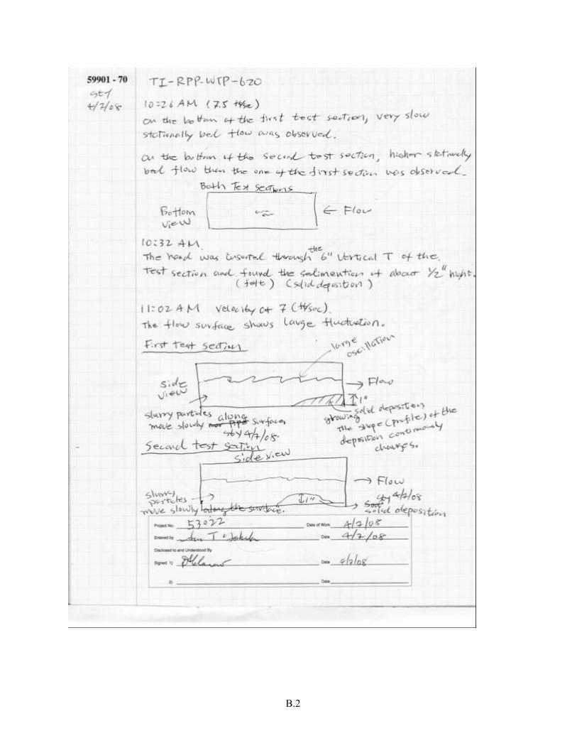
B.2

B.3

B.4

B.5

B.6

B.7

B.8

B.9

B.10

B.11

B.12

B.13

B.14

B.15

B.16
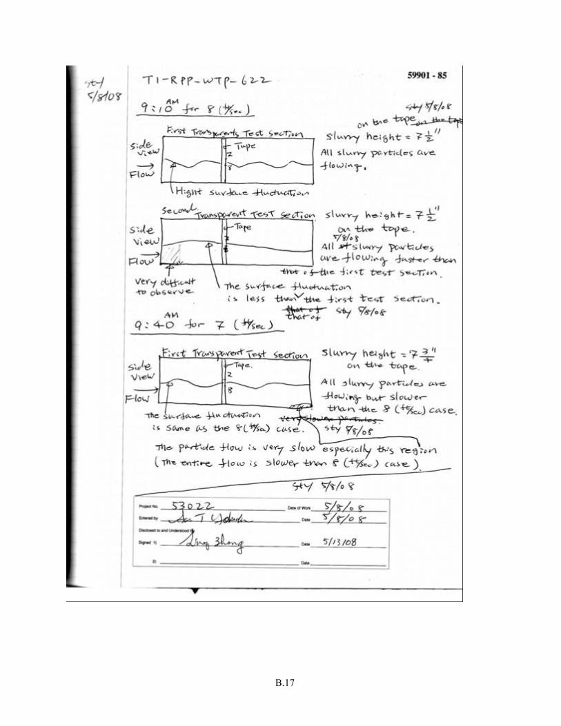
B.17

B.18

B.19

B.20

B.21

B.22

B.23
PNNL-17973 WTP-RPT-178 Rev. 0
Distr. 1
Distribution No. of Copies ONSITE 2 Bechtel National, Inc.
WTP R&T Docs (2) H4-02
5 Pacific Northwest National Laboratory H. E. Adkins K7-15 M. J. Minette P7-25 D. E. Kurath K3-52 S. T. Yokuda K7-15 Project Files K3-52 Information Release (pdf)