DP2009/12

A Quarterly Post-World War II Real GDP

Series for New Zealand

Viv B. Hall and C. John McDermott

November 2009

JEL classification: C22, C82, E01, E32

www.rbnz.govt.nz/research/discusspapers/

Discussion Paper Series

ISSN 1177-7567

DP2009/12

A Quarterly Post-World War II Real GDP Series for

New Zealand∗

Viv B. Hall and C. John McDermott†

Abstract

There are no official quarterly real GDP estimates for New Zealand, for theperiod prior to 1977. We report the development of a seasonally adjustedseries for a period of more than 60 years from mid-1947, and evaluate statis-tical properties. The series were developed by linking quarterly observationsfrom two recent official series to temporally disaggregated observations foran earlier time period. Annual real GDP series are disaggregated, usingthe information from two quarterly diffusion indexes, developed by Haywoodand Campbell (1976). Three econometric models are used: the Chow andLin (1971) model that disaggregates the level of GDP; and the Fernandez(1981) and Litterman (1983) models that disaggregate changes in GDP. Ourpreferred quarterly series is based on results generated from the Chow-Linmodel. We assess movements in the new series against qualitative findingsfrom New Zealand’s post-WWII economic history.

∗ The Reserve Bank of New Zealand’s discussion paper series is externally refereed. Theviews expressed in this paper are those of the author(s) and do not necessarily reflectthe views of the Reserve Bank of New Zealand. This paper is an updated version ofour earlier paper published as Motu Working Paper 07-13. We thank Arthur Grimes,Glenn Otto and Ozer Karagedikli for perceptive comments, and Brian Easton for hisvery helpful insights on key data periods. We are also grateful to Brian for supplyinghis Haywood and Campbell diffusion index data.

† Viv Hall (corresponding author), Victoria University of Wellington, School ofEconomics and Finance, PO Box 600, Wellington, New Zealand. Email ad-dress:viv.hall@vuw.ac.nz, John McDermott, Reserve Bank of New Zealand and Vic-toria University of Wellington, 2 The Terrace, PO Box 2498, Wellington, New Zealand.Email address: john.mcdermott@rbnz.govt.nz.ISSN 1177-7567 c©Reserve Bank of New Zealand

1 Introduction

The performance of the post-World War II (WWII) New Zealand economycannot be assessed effectively, without credible quarterly real GDP data thatspans a sufficiently long time period. This is so, whether one’s primary pur-pose is to establish classical business cycle turning points, evaluate competingtheories of the business cycle, or assess the impacts of various governmentpolicies and external shocks.

At present, there are no official quarterly real GDP estimates for New Zealand,for the period prior to 1977. The current official chain-linked series of quar-terly GDP goes back only to 1987. The span of time covered by this dataincludes only two completed classical business cycles and is thus inadequatefor establishing classical business cycle turning points and associated clas-sical cycle characteristics. There is a non-chain-linked series provided byStatistics New Zealand (SNZ) that covers the period 1977 to 1987 that al-lows researchers a little more leeway, but this span can still provide only fourcompleted cycles.

Annual data on New Zealand GDP back to 1955 is available from SNZ, butannual data is of rather limited use when it comes to establishing quarterlyclassical business cycle turning points. In addition to estimates availabledirectly from SNZ there are a number of unofficial estimates of annual GDPcovering more historical periods, including those of Lineham (1968), Hawke(1975), Easton (1990), and Rankin (1991).1 Most of these estimates are forthe period prior to WW II, and are therefore not directly relevant for thisstudy. The exception is the series provided by Easton (1990), covering theperiod 1913/14 to 1976/77. For the immediate post-WWII period, the onlyindicators available on a quarterly basis for broadly-based economic activitymovements are the diffusion indexes estimated by Haywood and Campbell(1976). These cover the period 1947 to 1974, and so the farthest we canpotentially backcast quarterly GDP is to 1947.

The primary object of this paper is therefore to develop a quarterly seasonallyadjusted real GDP series for New Zealand’s post-WWII period, by linkingrecent official quarterly observations to temporally disaggregated observa-tions for an earlier time period. The disaggregation is based on techniquesthat use seasonally adjusted indicator series which are available at a higherfrequency and are related as closely as possible to the series of interest.

1 Briggs (2003) provides a good summary of what each of these estimates involves andthe estimates are available on Statistics New Zealand’s long-term data series webpage(see http://www.stats.govt.nz/tables/ltds/default.htm).

1

Temporal disaggregation is commonly resorted to by researchers when officialstatistical agencies are unable to provide data at a required frequency. Themethod has also been used by official statistical agencies themselves whendirect estimation methods are unavailable.2

The remainder of the paper is as follows. Section 2 summarises the infor-mation available on economic activity in the New Zealand economy over thepost-WWII era. Section 3 sets out the Chow and Lin (1971) and relatedmethods for temporal disaggregation of the annual GDP data. Section 4explains the splicing of the new quarterly estimates for the period 1947 to1979, to official quarterly estimates for the period 1977 to 2008. Section5 evaluates statistical properties of the series, and their relative usefulnessfor business cycle analysis and policy appraisal. Section 6 concludes. Thequarterly seasonally adjusted data for our preferred series, based on resultsgenerated from the Chow-Lin model, are presented in Appendix Table A4.

2 The Data

2.1 The Source GDP Data

Our new quarterly real GDP time series covers the post-WWII sample period,1947q2 to 2008q3. Its construction has involved piecing together data fromvarious sources, and scaling the linked series to a 1995/96 base.

We use SNZ’s System of National Accounts series SNB, in 1991/92 prices,for the period 1977q2 to 1987q1. This seasonally adjusted series is not chain-linked. Their current series SNC, in 1995/96 prices, is chain-linked, and itsseasonally adjusted observations are used for the period 1987q2 to 2008q3.

For the period 1947 to 1977, however, annual observations obtained fromSNZ’s long-term data series webpage, had to be the starting point. For 1947to 1955, these observations are based on annual growth rates presented inEaston (1990), and for 1955 to 1977, the source is SNZ’s annual SNB series(1991/92 base). Growth rates of the annual series are shown in Figure 1 for

2 Proietti (2006, p 357) reports that “ ... a large share of the Euro area quarterly grossdomestic product is actually estimated by disaggregating annual data.” Ciammola, DiPalma, and Marini (2005, p 6) cite Italy, France, and Belgium as specific examples.SNZ use temporal disaggregation rather differently. Where data from different sourcesare used for the Annual and Quarterly National Accounts, they use a ‘benchmarking’process (see Bloem et al, 2001, pp 5-7), to ensure preliminary quarterly estimates areconsistent with the annual growth rates.

2

the years 1947 to 1979. Four periods involving negative economic growth caneasily be detected: 1949, 1952-53, 1968, and 1977-79.

Figure 1Growth Rate of Annual GDP (year ending March, 1947 to 1979 )

-6.00

-1.00

4.00

9.00

14.00

1947 1950 1953 1956 1959 1962 1965 1968 1971 1974 1977

Source: Statistics New Zealand’s long-term data series webpage,(see http://www.stats.govt.nz/tables/ltds/default.htm).

2.2 The Related Quarterly Series

Two diffusion indices constructed by Haywood and Campbell (1976) pro-vide the best information available on quarterly fluctuations in aggregateeconomic activity. For the period 1947q1 to 1974q4, from 63 seasonally ad-justed time series indicators3, they construct a weighted classical cycle indexand a weighted amplitude adjusted index4. The weights are based on each

3 For seasonal adjustment details, see Haywood and Campbell (1976, p 5, Chart A).4 The approach used for amplitude adjustment is similar to that of Shiskin (1961). Hay-

wood and Campbell’s computer programme also calculated deviation (or growth) cy-cles. Further details on their methodology are available in Haywood and Campbell(1976, ss 2, 3 and 4).

3

series’ relative economic significance, with consideration also being given tothe importance of the sector to which each series belongs.

Construction of the weighted classical cycle is based on the direction series

skt =

1, zkt > zk,t−1

0, zkt = zk,t−1

−1, zkt < zk,t−1

(1)

where zkt is the value of the kth time series indicator and sk1 = 0. Theweighted classical cycle index is then defined as

xt =t∑

i=1

K∑k=1

atskt (2)

for t = 1 to T , where ak is the relative weight of the kth indicator. Theweighted amplitude adjusted classical index is defined in a similar manner,except for the adjustment for the relative amplitudes of the indicator series.The underlying indicators and the weights used by Haywood and Campbell(1976) are shown in Appendix Tables A1 to A3.

The diffusion indices of Haywood and Campbell (1976, Tables 13 and 14, p22) end in 1974, and so leave us with a three year gap until the quarterlyGDP series start. Fortunately, however, the New Zealand Institute of Eco-nomic Research (NZIER) updated the weighted static deviation cycle indexof Haywood and Campbell (1976, Table 16, p 23) for a number of years, andpresented the outcomes in its Quarterly Predictions through till 1979. Thedeviation cycle index is closely related to the classical cycle index, and soafter further computation we were able to produce observations covering thenext three years. The difference between the classical and deviation cycleindices is that the deviation cycle is the aggregation of a direction indicatorof each indicator series. It takes on values of +1, 0% , or −1, dependingon whether a particular month’s deviation cycle was above, the same, orbelow its trend value. As such, the deviation cycle measure is suitable fordating growth cycles rather than classical cycles. This deviation cycle serieswas successfully matched by Kay (1984) to the NZIER’s surveyed BusinessOpinion measure of capacity utilization (CUBO), and in its extended formwas used by Easton (1997), to date turning points in growth cycles in theNew Zealand economy.

However, by assuming a trend consistent with the classical indices of Hay-wood and Campbell (HC), we were able to use the weighted static deviation

4

cycle index to extend both the weighted classical index and the weighted am-plitude adjusted classical index out to 1979q1. The assumed trend growthin both diffusion indices was 2.3 percent per annum, based on the averagegrowth rate over the period 1947 to 1974. These extended classical indicesare shown in Figure 2.

Figure 2Extended Haywood and Campbell Diffusion Indices (1947q1 to1981q1 )

0

1000

2000

3000

4000

5000

6000

1947 1949 1951 1953 1955 1957 1959 1961 1963 1965 1967 1969 1971 1973 1975 1977 1979

Weighted Amplitude Adjusted Classical Cycle Index

Weighted Classical Cycle Index

Source: Haywood and Campbell (1976), Easton (1997) and authors’ calculations.

3 Temporal Disaggregation Methods

The problem we face is that for the period 1947 to 1977 we have only annualreal GDP data, but would like quarterly data. The temporal disaggregationmethods most commonly used are those of Chow and Lin (1971), Fernandez(1981) and Litterman (1983)5. A key reason for their popularity for obtain-ing estimates of the desired high frequency data from low frequency data,is that they use relatively simple regression methods, dependent on a single

5 Proietti (2006) has investigated the potential use of state space methods for temporaldisaggregation purposes. He also refers to, but did not evaluate the multivariate timeseries approaches of Harvey and Chung (2000) and Moauro and Savio (2005). None ofthese methods seems to have been widely used yet.

5

autoregressive parameter. In this section, we therefore explain briefly thekey features of, and differences between, these methods, and present corre-sponding quarterly real GDP estimates.

The method most often used is that of Chow-Lin. It can be used to generateany higher frequency estimates from lower frequency source data (subjectto available higher frequency indicators), but from this point we restrictourselves to considering the problem of moving from annual data to quarterlydata.

Let y be a (4n × 1) vector of the unknown quarterly series. Let X be a(4n× p) vector of related series. For the current application p = 1. Assumethere exists a multiple regression of the form

y = Xβ + u (3)

where u is a vector of disturbances such that E[u] = 0, E[uu′] = V . Let i bea (4× 1) vector of ones so that C = In⊗ i′4 is an (n× 4n) matrix convertingquarterly into annual observations That is,

ya = Cy and Xa = CX. (4)

An optimal (in the BLUE sense) estimator y of y is given by

y = Xβ + V C ′(CV C ′)−1C(ya −Xaβ) (5)

whereβ = (X ′

a(CV C′)−1Xa)

−1X ′a(CV C

′)−1ya. (6)

A practical problem is that, in general, V is unknown and must be estimated.Chow-Lin assume a simple autoregressive structure for the disturbances ofthe form

ut = ρut−1 + εt (7)

where E[εt] = 0, E[ε2t ] = σ2. The resulting covariance matrix V has the

Toeplitz form

V =σ2

1− ρ2

1 ρ ρ2 · · · ρ4n−1

ρ 1 ρ · · · ρ4n−2

ρ2 ρ 1 · · · ρ4n−3

......

.... . .

...ρ4n−1 ρ4n−2 ρ4n−3 · · · 1

(8)

6

and the covariance of the annual residuals is then given by Va = CV C ′. Thefirst-order autocorrelation of the annual disturbances ρa is related to ρ in thefollowing way

ρa = f(ρ) =ρ (ρ+ 1) (ρ2 + 1)

2

2 (ρ+ ρ2 + 2). (9)

An iterative procedure can therefore be used to obtain an estimate of ρ. Firstregress ya on Xa to get an estimate of u1

a and then regress u1a on the first lag

of u1a to obtain an estimate ρ1

a. Obtain an estimate of ρ using ρ1 = f−1(ρ1a).

Take this estimate and form a set of annual regression residuals using

u2a = ya −Xa

[(X ′

a(CV1C′)−1Xa)

−1X ′a(CV1C

′)−1ya

](10)

where V1 is the Toeplitz matrix based on the estimate ρ1. From these residu-als compute a new estimate ρ2

a and thus a new ρ2 is obtained via the inversefunction of f(ρ). Continue until convergence is achieved. Plugging thesefinal estimates into (5) yields the best linear unbiased estimate of quarterlyreal GDP.

As long as the first order autocorrelation coefficient is positive the iterativeprocedure will converge. It is important to verify this condition before tryingto apply the Chow-Lin procedure. It is also important to verify that theChow-Lin regression model (3) forms a cointegrating relationship when theunderlying data contain stochastic trends.

We estimate the Chow-Lin regression over the period 1947q2 to 1979q1.Strictly speaking we need to estimate the regression only over the period1947q2 to 1977q1, since we have quarterly GDP data starting from 1977q2.However joining the Chow-Lin estimates at 1977 is problematic for two rea-sons: (i) SNZ quarterly and annual series do not match for this year; and (ii)

7

the SNZ growth estimates for this year are in dispute.6 Thus in order to spliceour new quarterly estimates to the existing quarterly estimates without anyawkward discontinuities we use the sample up to 1979q1 for the Chow-Linregression.

We consider the two cases: (i) the related series is the HC weighted classicaldiffusion index (denoted unadjusted); and (ii) the related series is the HCweighted amplitude adjusted classical diffusion index (denoted adjusted).Table 1 reports the estimated values of the autoregressive coefficient (for bothannual and quarterly data) and a residual based test of cointegration, usingthe augmented Dickey Fuller (ADF) statistic. In the first case, the necessaryconditions that the autoregressive coefficient is positive, and the Chow-Linregression is cointegrated, are satisfied. However, in the second case, whilethe autoregressive coefficient is positive, it is so close to the unit root value ofone that the cointegration condition is violated. For the Chow-Lin regressionmethod, the amplitude adjusted series can therefore be rejected in favour ofthe series without adjustment.

When the cointegration condition fails, alternative methods proposed by Fernandez (1981) and Litterman (1983) are considered potentially more suitable.The salient characteristic of the Fernandez-Litterman methods involves tem-

6 The Statistics New Zealand production-based real GDP series SNBA.2SAZAT re-ports annual growth of -2.6 percent for the year ending 31 March 1978. The se-ries was discontinued in June 2000. An earlier series SNBA.SX9 (discontinued inMarch 1985) shows annual growth of -3.5 percent. Brian Easton suggests thateven the -2.6 percent figure appears implausibly low, given other macroeconomicand sectoral data. (See “The 1977/78 Downturn in the New Zealand Economy”http://www.eastonbh.ac.nz/?p=776.) In personal communication, Brian Easton hasadvised us that the exaggerated contraction is due to the adoption of a new inventoryseries with no overlap between surveys. The problem is even worse when one examinesthe quarterly data. The official real GDP index (SNBQ.SY299) records growth ratesfor September 1977, December 1977 and March 1978 as -2.1 -4.3, and 0.0 percent, re-spectively. Such a substantial decline in output would surely have been noticed at thetime as a particularly major contraction, and have been widely commented on. Havingthe underlying surveys change and a new quarterly series start during a significantcontraction makes unravelling the truth of the matter impossible. So, given that thenegative quarterly official statistics for the second half of 1977 are almost certainlyimplausibly low, we have not including those observations in our series. Instead wehave used the estimates from the Chow-Lin procedure based on the annual data andthe Haywood and Campbell related indicators. This still leaves a large contractionfor the March 1978 year consistent with the official annual data. In generating ournew quarterly GDP estimates we believe it is important to stay as close as possible toofficial statistics, while at the same time recommending caution to potential users, whomay if they wish apply their own adjustments. For example, Brian Easton has guessedthe annual March 1978 contraction to be more like 1 to 1.5 percent.

8

Table 1Chow-Lin Regression Results (sample period 1947q2 to 1979q1 )

Statistic Unadjusted Adjusted

β0 5.575 6.411β1 3.109 2.282ρa 0.869 0.968ρ 0.949 0.988ADF Test −4.844 −2.116

Notes: The 5% critical values for the cointegration test is −3.385 from MacKin-non(1991). The results, for when the HC weighted classical diffusion index is usedas the related series, are shown in the column labelled unadjusted. Results forwhen the HC weighted amplitude adjusted classical diffusion index is used as therelated series, are shown in the column labelled adjusted.

poral disaggregation of the annual changes into quarterly changes. Thus wehave the regression model

∆y = ∆Xβ + u (11)

where ∆ denotes the first difference operator and we have the following for-mulation for the disturbance terms

ut = ut−1 + et (12)

whereet = ψet−1 + εt. (13)

The Fernandez model is the special case when ψ = 0. Under this assumptionthe resulting covariance matrix V has the form (D′D)−1 where the 4n× 4nmatrix D is given by

1 0 0 · · · 0 0−1 1 0 · · · 0 00 −1 1 · · · 0 0...

......

. . ....

...0 0 0 · · · −1 1

. (14)

Plugging the above formula into (5) yields the Fernandez estimate of quar-terly real GDP. We estimate the Fernandez regression over the period 1947q2to 1979q1. Again we consider the two cases: (i) the related series is the HC

9

Table 2Fernandez Regression Results (sample period 1947q2 to 1979q1 )

Statistic Unadjusted Adjusted

β0 6.518 6.360β1 2.015 1.805ρa −− −−ρ −− −−ADF Test −1.290 −1.228

Notes: See Table 1.

weighted classical diffusion index (denoted unadjusted); and (ii) the relatedseries is the HC weighted amplitude adjusted classical diffusion index (de-noted adjusted). Table 2 reports the estimated values of the autoregressivecoefficient (for both annual and quarterly data). Given that the value of ρwas set to unity, the tests for cointegration between the estimated quarterlyseries and the related series are rejected.

Finally, the Litterman (1983) method of temporally disaggregation is also apossible option. The Litterman model adds the problem of estimating theparameter ψ. In this case the resulting covariance matrix V has the form(D′H ′HD)−1 where the 4n× 4n matrix H is given by

1 0 0 · · · 0 0−ψ 1 0 · · · 0 00 −ψ 1 · · · 0 0...

......

. . ....

...0 0 0 · · · −ψ 1

. (15)

The first-order annual serial correlation coefficient, ψa, is related to thequarterly coefficient, ψ. To calculate this relationship one sets ψa equalto the ratio of the off-diagonal element to the diagonal element of the matrixQH−1H−1′Q′ (Silver, 1986), where Q = ∆CD−1 and the n × n matrix ∆ isgiven by

1 0 0 · · · 0 0−1 1 0 · · · 0 00 −1 1 · · · 0 0...

......

. . ....

...0 0 0 · · · −1 1

. (16)

10

Table 3Litterman Regression Results (sample period 1947q2 to 1979q1 )

Statistic Unadjusted Adjusted

β0 6.624 6.503β1 1.321 1.279ψa 0.633 0.633ψ 0.950 0.950ADF Test −0.956 −0.935

Notes: See Table 1.

Plugging this formula for V , together with the final estimate of ψ, into (5)yields the Litterman estimate of quarterly real GDP. We estimate the Lit-terman regression over the period 1947q2 to 1979q1, again using both theunadjusted and adjusted related series of HC. The estimated coefficient forthe regression using the unadjusted or the adjusted related series are broadlysimilar. As with the Fernandez regression the estimated quarterly GDP seriesis not cointegrated with the related series.

The Chow-Lin, Fernandez, and Litterman-based quarterly real GDP growthrate estimates, for the unadjusted HC diffusion index, are presented in Figure3. Visual inspection reveals the differences to be almost imperceptible. Theonly visible difference is that the amplitudes of the Chow-Lin series are afraction higher. Overall, therefore, including when viewed in the context ofthe annual growth rates presented in Figure 1, the temporally disaggregatedseries from all three methods seem to provide potentially valuable quarterlyreal GDP information.

4 Splicing the Data

One final computation remains. That is to combine the temporally disaggre-gated and official quarterly GDP series, to make a complete time series. Theestimated GDP observations for the period 1947q2 to 1979q1, and the SNBseries for the period 1979q2 to 1987q1 are converted into 1995/96 prices, soas to match the base year for the 1987q2 to 2008q3 SNC series.

The resulting quarterly series, covering the period 1947q2 to 2008q3, can besubdivided into four periods of potentially distinct quality and consistency.Issues involving credibility of the data for 1977, and the extent to which the

11

Figure 3Quarterly Real GDP Growth Estimates, from Chow-Lin,Fernandez and Litterman Methods (1947q2 to 1979q1, unadjustedHC series)

-4

-3

-2

-1

0

1

2

3

4

5

6

1949q1 1951q1 1953q1 1955q1 1957q1 1959q1 1961q1 1963q1 1965q1 1967q1 1969q1 1971q1 1973q1 1975q1 1977q1

Chow-Lin FernandezLitterman

annual and quarterly observations match for that year, were summarised insection 2 above, and results from testing for structural breaks (whether froma key economic event or due to different methods of series construction) arepresented below in section 5.

The first period, 1947q2 to 1954q1, potentially has the lowest quality data,being generated from temporally disaggregated unofficial annual estimates.This period also suffers from some very volatile fluctuations, associated withthe conversion of economic production from wartime to peacetime mode. Itfollowed World War II, and included the Korean War and associated woolboom, and the food rationing system still in place in the United Kingdom.At the time, the UK was still New Zealand’s major export destination.

The second period, 1954q2 to 1979q1, has data of somewhat of higher quality,in the sense that the annual data is based on official statistics. However,the quarterly track still contains an unknown degree of estimation error.

12

The closer the Haywood and Campbell diffusion index is to what actuallytranspired, the smaller this estimation error would be.

The quality of the third period data, from 1979q2 to 1987q1, is likely to bebetter still, since we no longer need to rely on a related indicator to assistwith estimating the quarterly track for GDP, and we can use the non-chain-linked series available from SNZ. Finally, the fourth period 1987q2 to 2008q3will have the highest quality data, since it is the current series of chain-linkeddata with SNZ preferred status.

The real GDP series for 1947q2 to 2008q3, based on the Chow-Lin unadjustedHC series estimates7, and the corresponding Fernandez- and Litterman-basedestimates, are presented in Figure 4. Visually, there are no detectable differ-ences between these natural log series.

But before proceeding to express preference for a Chow-Lin, Fernandez, orLitterman-based series, whether for the purposes of business cycle analysisor the dating of classical business cycle turning points, we examine the series’key statistical properties, and test for any structural breaks.

5 Series Evaluation

5.1 Unit Root and Cointegration Tests

Each of the four GDP series show strong trending behaviour. Unit roottests reported in Table 4 indicate that at the 5 percent significance level thehypothesis of a unit root in the level of GDP cannot be rejected, implyingthere is a stochastic trend in the data. The hypothesis of a unit root isrejected at the 5 percent level for the first difference of the series, implyingall four series are integrated of order one.

Whatever estimation method or related series are used we would expect thatover a long enough span of data our estimated GDP series should informus about the long run trends in the data. That is, each of the estimatedseries should be cointegrated with each other. Table 5 reports the Johansentrace statistics for cointegration statistics, and the results indicate that thereare five cointegrating equations at the 0.05 level. The five estimated coin-tegrating vectors are (1,−1) up to three decimal places. Thus, the most

7 Recall, from the cointegration test results presented in Table 1, that for the Chow-Linmethod, the amplitude adjusted series could be rejected in favour of the series withoutadjustment.

13

Figure 4Quarterly Real GDP Growth Estimates, from Chow-Lin,Fernandez and Litterman Methods (1947q2 to 2008q3, naturallogs)

8.5

8.7

8.9

9.1

9.3

9.5

9.7

9.9

10.1

10.3

10.5

1951q1 1955q1 1959q1 1963q1 1967q1 1971q1 1975q1 1979q1 1983q1 1987q1 1991q1 1995q1 1999q1 2003q1 2007q1

Chow-Lin FernandezLitterman

Source: SNZ from 1979q2 to 2008q3, and estimates based on Chow-Lin, Fernandez,and Litterman regressions for the period 1947q2 to 1979q1.

basic requirement from our estimation methods, is that we obtain consistentresults on the long run trends in the data.

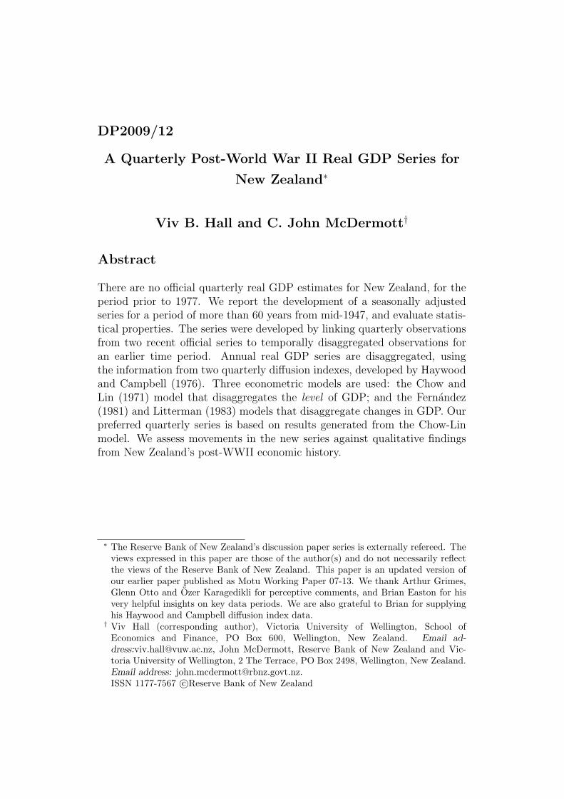
Next we compare the correlations of the growth rates (reported in Table 6)to see if different methods of disaggregating the annual data might producedifferent first difference growth cycles. We observe very high correlations be-tween growth rates irrespective of which estimation method or which relatedseries is used.

Both the cointegration test for the levels data, and the correlations of thegrowth rates, demonstrate that the choice of diffusion index used to convertannual series into quarterly series is largely immaterial. Therefore, for theremainder of the paper, we will report only the results generated from HC’sweighted classical cycle index. Results using the weighted amplitude adjusted

14

Table 4Unit Root Tests for Logarithms of GDP (sample 1947q2 to2008q3 )

Estimation method Related Series Levels First difference

Chow-Lin Unadjusted −1.998 −7.047Chow-Lin Adjusted −2.032 −7.066Fernandez Unadjusted −2.075 −6.720Fernandez Adjusted −2.065 −6.878Litterman Unadjusted −2.185 −6.552Litterman Adjusted −2.163 −6.593

Note: The 5% critical value is −3.429 (MacKinnion, 1991). The hypothesis of aunit root was tested against the alternative of a trend stationary process. The laglength for the unit root test was determined using the Akaike information criterionwith a maximum lag of 14.

Table 5Johansen Cointegration Test (sample 1947q2 to 1977q1 )

Hypothesised Number of Trace 5% CriticalCointegrating Equations Statistic Value

None* 410.0 95.8At most 1* 248.6 69.8At most 2* 163.9 47.9At most 3* 92.9 29.8At most 4* 33.0 15.5At most 5 0.3 3.8

Notes: The lag length for the cointegration test was 5, and was determined by usingthe Akaike information criterion with a maximum lag of 6. The model assumed alinear deterministic trend. * denotes significant at the 5% level.

15

Table 6Correlation of Growth Rates (sample 1947q2 to 1977q1 )

Series Chow-Lin Fernandez Litterman(unadj) (adj) (unadj) (adj) (unadj) (adj)

Chow-Lin(unadj) 1 0.964 0.981 0.965 0.945 0.942Chow-Lin(adj) 1 0.953 0.996 0.934 0.971Fernandez(unadj) 1 0.970 0.985 0.970Fernandez(adj) 1 0.958 0.985Litterman(unadj) 1 0.984Litterman(adj) 1

classical cycle index are almost identical.

5.2 Statistical Properties

In order to help establish the relative merits of the Chow-Lin, Fernandezand Litterman-based real GDP series, we summarize their stylised statisticalfacts. Tables 7 to 9 report statistics that summarize the properties of theseries, in terms of growth, volatility, normality, and persistence. One concernpotential users may have with the splicing of data generated by differentmethods is that the splicing may induce unsatisfactory properties in theseries. To check this, we also examine properties for the four sub-periodsreferred to above, corresponding approximately to the relative quality of thedata sub-period observations. Recall that these are as follows: period I,1947q2 to 1954q1; period II, 1954q2 to 1977q1; period III, 1977q2 to 1987q1;and period IV, 1987q2 to 2008q3. Naturally, the Full period is 1947q2 to2008q3.

For all three series, period II is the high growth period with a mean growthrate of about 0.9 percent per quarter (about 3.6 percent per year) while thelow growth period is period III with a mean growth rate of approximately0.4 percent per quarter (about 1.6 percent per year).

Period I was a time of extreme fluctuations in economic activity, with stan-dard deviations about twice the size of those for the sample as a whole. Therelatively benign periods for fluctuations in economic activity were periods IIand IV. Of more interest, is the volatility in the usual business cycle frequency(6 quarters to 32 quarters) which can be measured using the integrated nor-

16

Table 7Stylised Facts for GDP Growth (annual data converted to quar-terly using the Chow-Lin Model)

Statistic Sample PeriodPeriod I Period II Period III Period IV Full

Mean 0.548 0.909 0.403 0.624 0.686Median 0.299 1.001 0.198 0.716 0.766Std. Dev. 2.348 0.809 1.248 0.864 1.173Skewness 0.384 −0.475 0.109 −0.637 -0.015Kurtosis 2.661 2.766 3.002 4.298 5.614Jarque-Bera 0.796 3.668 0.079 11.860 69.800Half-life 2.941 0.711 0.372 0.535 0.915H(ω1, ω2) 0.831 0.448 0.413 0.343 0.400

Notes: The sample periods are: period I, 1947q2 to 1954q1; period II, 1954q2 to1977q1; period III, 1977q2 to 1987q1; and period IV, 1987q2 to 2008q3. The Fullperiod is 1947q2 to 2008q3. The Jarque-Bera statistic provides a test of normalitywhich has a χ2 - distribution with 2 degrees of freedom and thus a 5% critical valueof 5.991. The half-life is the length of time (in quarters) it takes for a shock toGDP growth to dissipate by half. The integrated normalised spectrum (H(ω1, ω2)provides the fraction of variance attributable to the business cycle frequency range6 quarters to 32 quarters.

malised spectrum (see for example Ahmed, Levin and Wilson (2004)). Theintegrated normalised spectrum for any band of frequencies can be estimatedusing

H(ω1, ω2) =

[ω2 − ω1

πΓ(0) +

2

π

T−1∑j=1

Γ(j)sin(ω2j)− sin(ω1j)

j

]/σ2 (17)

where Γ(j) represents the jth-order sample autocovariance and ω1 = π/16 andω2 = π/3 which corresponds to cycles of 6 to 32 quarters. The integratednormalised spectrum tells us that, for business cycle frequencies, the volatilityis similar for the 3 sub-periods II to IV, and for the Full period. The fact thatthe integrated normalised spectrum is higher in period I should be treatedwith some caution, given that it is only 28 quarters long.

The Jarque-Bera test for normality is clearly rejected for the full sample withstrong evidence of excess kurtosis. However, growth rates appear to follow anormal distribution in each sub-period, except for period IV. The rejection ofnormality seems to be due to the mixture of normals with different standard

17

deviations, rather than being drawn from a distribution with fat-tails.

Finally, we can examine the persistence of the innovation to growth usinga measure of the half-life, which is the length of time (in quarters) it takesfor a shock to GDP growth to dissipate by half, and is given by the formula|ln(0.5)/ ln(α)| ,where α is the parameter in an autoregressive model of orderone. A median-unbiased estimate of α was computed using the procedure ofAndrews (1993a). In general, the degree of persistence is small, with shocksdissipating by about half each quarter. The exception is period I which showsmore persistence. However, again we need to be cautious about reading toomuch into this result given the small sample size of this sub-period.

The stylised facts for the Chow-Lin, Fernandez and Litterman-based growthrate series are generally consistent across sub-periods. To this point, then,there is no compelling evidence to prefer one model over the other.

However, there are somewhat greater differences for period I, foreshadowedabove in section 4 as having potentially problematic observations associatedwith post-WWII exceptional events. This further suggests that considerablecaution should be exercised if observations from the beginning of the Fullsample are to be used. In fact, we recommend that for most statistical pur-poses the sample should be restricted to the period 1954q2 to 2008q3 becauseof the special feature imposed on the data by the changes in economic pro-duction following WWII and the Korean War. Treating these New Zealanddata observations in this way would be not be unusual, as in their macro-economic time series study of business cycle fluctuations in the US, Stockand Watson (1999) restricted their statistical analysis to the period 1953q1to 1996q4, for these very reasons.

5.3 Structural Breaks

To assess whether our splicing procedure has introduced any change in thegrowth rate or variance of the resulting series we apply the tests of Andrews(1993b) and Andrews and Ploberger (1994).

We test for a structural break in GDP growth using the regression

∆yt = µ+ εt. (18)

We also test for a structural break in the residual variance using the regression

ε2t = κ+ νt. (19)

18

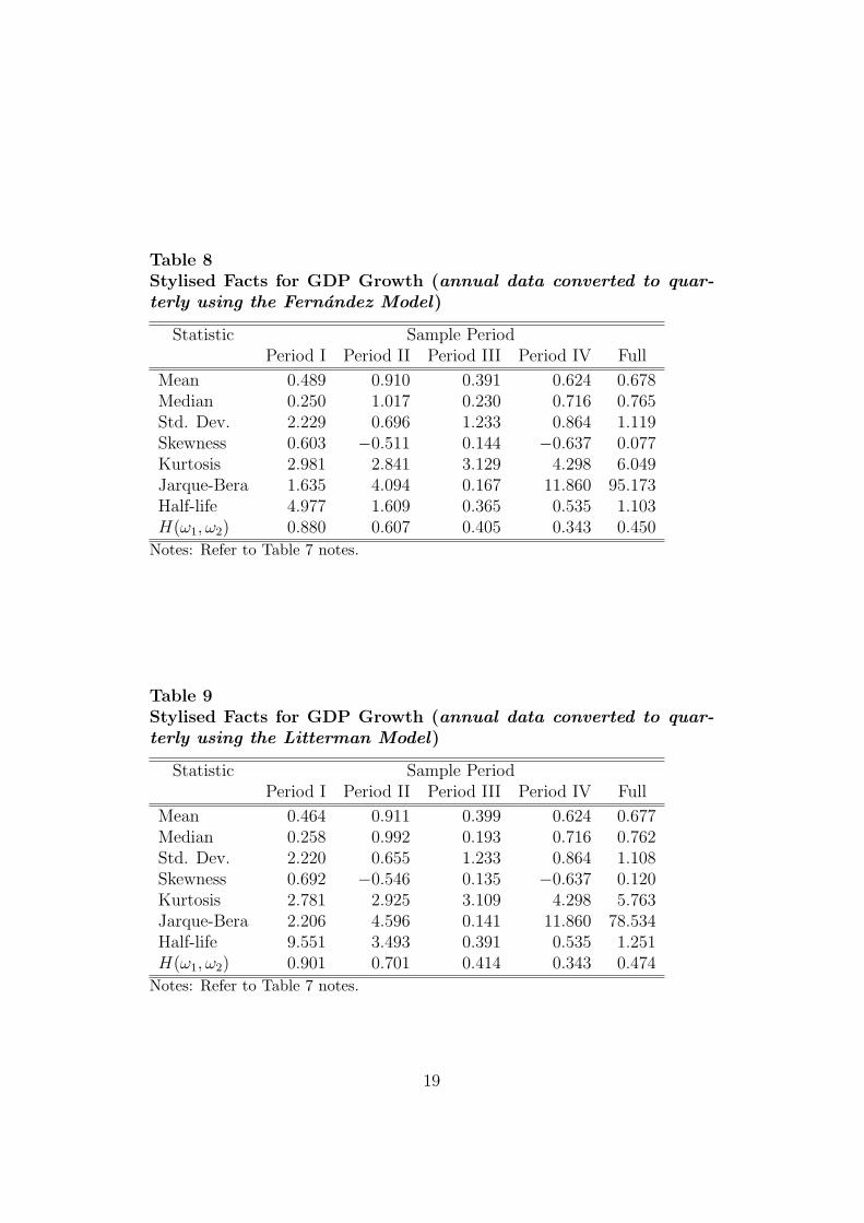
Table 8Stylised Facts for GDP Growth (annual data converted to quar-terly using the Fernandez Model)

Statistic Sample PeriodPeriod I Period II Period III Period IV Full

Mean 0.489 0.910 0.391 0.624 0.678Median 0.250 1.017 0.230 0.716 0.765Std. Dev. 2.229 0.696 1.233 0.864 1.119Skewness 0.603 −0.511 0.144 −0.637 0.077Kurtosis 2.981 2.841 3.129 4.298 6.049Jarque-Bera 1.635 4.094 0.167 11.860 95.173Half-life 4.977 1.609 0.365 0.535 1.103H(ω1, ω2) 0.880 0.607 0.405 0.343 0.450

Notes: Refer to Table 7 notes.

Table 9Stylised Facts for GDP Growth (annual data converted to quar-terly using the Litterman Model)

Statistic Sample PeriodPeriod I Period II Period III Period IV Full

Mean 0.464 0.911 0.399 0.624 0.677Median 0.258 0.992 0.193 0.716 0.762Std. Dev. 2.220 0.655 1.233 0.864 1.108Skewness 0.692 −0.546 0.135 −0.637 0.120Kurtosis 2.781 2.925 3.109 4.298 5.763Jarque-Bera 2.206 4.596 0.141 11.860 78.534Half-life 9.551 3.493 0.391 0.535 1.251H(ω1, ω2) 0.901 0.701 0.414 0.343 0.474

Notes: Refer to Table 7 notes.

19

Table 10Tests for Structural Change (sample period 1947q2 to 2008q3 )

Estimation method Exp Ave Sup Estimated Break

GDP growthChow-Lin 1.197 1.496 6.294 1975q2Fernandez 1.244 1.505 6.450 1975q2Litterman 1.207 1.469 6.338 1974q3

GDP varianceChow-Lin 57.045 16.700 124.316 1952q1Fernandez 53.022 13.810 116.609 1952q1Litterman 65.049 15.315 140.866 1952q1

Notes: Exp, Ave and Sup refer to the exponential, average and supremum teststatistics of Andrews and Ploberger (1994) and Andrews (1993b). The 5 percentcritical values are 2.06 (Exp), 2.88 (Ave), and 8.85 (Sup). The first 5 percent andlast 5 percent of the sample are excluded as possible break points. Thus the rangeof possible break points considered covers the period 1950q3 to 2005q1.

The estimated break dates reported in Table 10 are consistent with therebeing no clear evidence of breaks attributable to the splicing of official serieswhich have been compiled differently (which would be at 1987q1 and 1987q2),or to the splicing of temporally disaggregated and official series (which wouldbe between 1977q1 and 1979q1). The null of no break in the GDP growthseries cannot be rejected at the 5 per cent significance level, and the commonbreak date of 1952q1 for the GDP variance is consistent with material changesin economic activity, rather than with series-splicing or with chain-linkedversus non-chain-linked methodologies.

5.4 Link to New Zealand’s Post-WWII Economic His-tory

For the Chow-Lin, Fernandez and Litterman-based series, the cointegrationvector presented in section 5.1 has shown that the long run trends in the Fullsample series are consistent. The corresponding correlation of growth ratesfor their unadjusted series is also high, at 94.5 per cent or better.

Breaking the data by sub-periods reveals the biggest difference across timeoccurs in the variance of the growth rate over the immediate post-WWII

20

period to 1954q1. This provides further support to our recommendation insection 5.3 that, for most statistical purposes, the Full sample should beeither restricted to the period 1954q2 to 2008q3, or the earliest observationstreated with considerable caution. It is also consistent with the finding insection 5.3 of a structural break in all three series, at 1952q1.

But what of the relative merits of the Chow-Lin, Fernandez and Litterman-based levels of GDP series, for the purposes say of dating classical businesscycle turning points?8 Visual inspection of Figure 5 suggests, as expectedfrom the series’ common official data components, that they can clearly iden-tify the contractions of the early 1980s and 1990s, and the contraction asso-ciated with the Asian financial crisis and summer drought period of 1997-98.It is also the case that the series appear to behave very similarly for con-tractions around the ‘Black Budget’ of 1958, and the exchange rate crisis1966-67. A possible quibble, though, is that the slightly different amplitudesof the cycles have the potential to identify slightly different short periods ofnegative growth. Such minor differences could make the dating of any as-sociated growth or classical business cycle turning points sensitive to whichmethod has been employed to disaggregate the GDP series.

Overall, there is very little difference in the temporally disaggregated obser-vations estimated from the three methods. However, on balance, we preferto use the Chow-Lin-based series for most purposes. This preference is basedon the fact that the cointegration test cannot be rejected for the Chow-Linregression, implying there is minor specification error in the Fernandez andLitterman regressions.

6 Conclusion

We have developed a new quarterly seasonally adjusted real GDP series forpost-WWII New Zealand, spanning the period 1947q2 to 2008q3. It containstwo short periods of observations, which will remain somewhat controversial,namely 1947q2 to 1953q3, and 1977. Despite this, we believe this new seriesfor a considerably longer period than has previously been available, will bevaluable for a range of purposes. These include the identification of classi-

8 A new ‘benchmark’ set of Classical business cycle turning points, for the period 1947q2to 2006q2, and reference to the associated key events in New Zealand’s economic history,are reported in Hall and McDermott (2009). Utilising the series for 1947q2 to 2008q3presented in this paper adds a further ‘benchmark’ turning point to those presented inHall and McDermott’s (2009) Table 1 - a Classical business cycle peak at 2007q4.

21

cal business cycle turning points, the establishment of a more robust set ofbusiness cycle characteristics, and assistance with assessing the impacts ofvarious government policies and external shocks.

Our series were developed by linking quarterly observations from two recentofficial series to temporally disaggregated observations for an earlier timeperiod. Annual official and non-official real GDP series were disaggregatedusing the information from two quarterly diffusion indexes developed by Hay-wood and Campbell. Three econometric methods were used: the Chow-Linmodel that disaggregates the level of GDP; and the Fernandez and Littermanmethods that disaggregate the change in GDP.

Statistical properties of the series were evaluated, and movements in the newseries checked against qualitative findings from New Zealand’s post-WWIIeconomic history.

Consistent results were obtained for the long run trends in all three series,and this suggests any one of the series could be used for measuring economicgrowth, or testing growth theories. However, when it comes to measuringbusiness cycle fluctuations, results associated with the early post-War yearsmight be somewhat sensitive to which series is used. The quarterly obser-vations prior to 1954 reflect the special nature of the fluctuations in thatperiod, and the probability of these being repeated in the near future maynot be high. So, most users would be wise to discard from their sample thequarterly observations prior to 1954. We have done this when estimatingMarkov-switching growth models for post-War New Zealand, but for dat-ing classical business cycle turning points we have preferred the Full samplequarterly series based on results generated from the Chow-Lin model.

The quarterly seasonally adjusted data for this preferred series are presentedin Appendix Table A4.

References

Ahmed, S, Levin, A and B Wilson (2004), “Recent U.S. Macroeconomic Sta-bility: Good Policies, Good Practices, or Good Luck?” Review of Economicsand Statistics, 86, 824-832.

Andrews, D (1993a), “Exactly Median-Unbiased Estimation of First OrderAutogressive/Unit Root Models,” Econometrica, 61, 139-165.

22

Andrews, D (1993b), “Tests for Parameter Instability and Structural Changewith Unknown Change Point,” Econometrica, 61, 821-856.

Andrews, D and W Ploberger (1994), “Optimal Tests When a Nuisance Para-meter Is Present Only Under the Alternative,” Econometrica, 62, 1383-1414.

Bloem, A, Dippelsman, R and N Maehle (2001), Quarterly National AccountsManual: Concepts, Data Sources, and Compilation, International MonetaryFund, Washington DC.

Briggs, P (2003), Looking at the Numbers: A view of New Zealand’s eco-nomic History, New Zealand Institute of Economic Research, Wellington,New Zealand.

Chow, G and A-L Lin (1971), “Best Linear Unbiased Interpolation, Dis-tribution, and Extrapolation of Time Series by Related Series”, Review ofEconomics and Statistics, 53 (4), 372-375.

Ciammola, A, Di Palma, F and M Marini (2005), “Temporal DisaggregationTechniques of Time Series by Related Series: A comparison by a Monte Carloexperiment”, Eurostat, Working Paper.

Easton, B (1990), A GDP deflator series for New Zealand 1913/4-1976/7,Massey Economic Papers, 8 (B9004), December.

Easton, B (1997), In Stormy Seas: The Post-War New Zealand Economy,Dunedin: University of Otago Press.

Fernandez, R (1981), “A Methodological Note on the Estimation of TimeSeries”, Review of Economics and Statistics, 63, 471-476.

Hall, V B and C J McDermott (2009), “The New Zealand Business Cycle”,Econometric Theory, 25, 1050-1069.

23

Harvey, A and C Chung (2000), “Estimating the Underlying Change in Un-employment in the UK”, Journal of the Royal Statistics Society, Series A,163, 303-339.

Hawke, G (1975), “Income Estimation from Monetary Data: Further Explo-ration”, Review of Income and Wealth, 301-307.

Hawke, G (1985), The Making of New Zealand, an economic history, Cam-bridge: Cambridge University Press.

Haywood, E (1972), The dating of post war business cycles in New Zealand1946-1970, Reserve Bank of New Zealand Research Paper, No. 4.

Haywood, E and C Campbell (1976), The New Zealand economy: measure-ment of economic fluctuations and indicators of economic activity, ReserveBank of New Zealand Research Paper, No. 19.

Kay, L (1984), “The utilisation of capacity measure and the reference busi-ness cycle”, New Zealand Institute of Economic Research, Quarterly Surveyof Business Opinion, No. 93, 26-29.

King, M (2004), The Penguin History of New Zealand, Auckland: PenguinBooks.

Lineham, B (1968), “New Zealand’s Gross Domestic Product 1918/38”, NewZealand Economic Papers, 2, 15-36.

Litterman, R (1983), “A Random Walk, Markov Model for the Distribu-tion of Time Series”, Journal Business and Economics, 1, 169-173.

MacKinnon, J (1991), “Critical Values for Cointegration Tests”, in R Engleand C Granger (eds.) Long-Run Economic Relationships: Reading in Coin-tegration, Oxford University Press, Oxford.

Moauro, F and G Savio (2005), “Temporal Disaggregation using MultivariateStructural Time Series Models”, Econometrics Journal, 8, 214-234.

24

Proietti, T (2006), “Temporal Disaggregation by State Space Methods: Dy-namic Regression Methods Revisited”, Econometric Journal, 9, 357-372.

Rankin, K (1992), “Gross National Product Estimates for New Zealand 1859-1939”, Working Paper series 1/91, Graduate School of Business and Govern-ment Management, Victoria University of Wellington.

Shiskin, J (1961), Signals of Recession and Recovery, NBER, New York, 43-44.

Silver, J (1986), “Two Results Useful for Implementing Litterman’s Proce-dure for Interpolating a Time Series”, Journal of Business and EconomicsStatistics, 4, 129-130.

Stock, J and M Watson (1999), “Business Cycle Fluctuations in US Macro-economic Time series”, in J Taylor and M Woodford (eds.) Handbook ofMacroeconomics, Volume 1A, Elsevier North Holland, Amsterdam.

25

Appendix

26

Table 11Employment and Production Indicators

Haywood and Campbell IndicatorsIndicator Weights

Index of effective weekly wage rate, adult males 4Real net salary and wage payments 9Labour placements ×− 1 3Notified vacancies 9Registered unemployed ×− 1 9Employment in industry, female 5Employment in industry, male 5Employment in industry, total 10Industrial disputes, working days lost 1Meat production 2Gas production 3Electricity generation 5Production of cheese 2Production of butter 2Electric ranges 4Washing machines 4Refrigerators 4Paper 3Plywood production, 3/16 in. basis 3Chemical fertilisers, total make 4Cement 4Passenger cars assembled 5Trucks, vans and buses assembled 6Beer production 1RNBZ volume of domestic manufacturing production index 10

Source: Haywood and Campbell (1976, Table 1, p 6).

27

Table 12Investment, External, Transport, and Domestic Trade Indicators

Haywood and Campbell IndicatorsIndicator Weights

Building permits issued 9Wholesale turnover of machinery 6Manufacturers’ stocks, including primary processing 3Manufacturers’ stocks, excluding primary processing 9Terms of trade 5Exports, total f.o.b. 8Imports, total c.d.v. 8Surveyed import orders 6Surveyed import payments 6Current account balance 8Government railways, net ton-miles run 2Government railways, passenger journeys, motor 2Government railways, passenger journeys, railway 2Civil aviation, freight tonne-kilometres 2Civil aviation, passenger kilometres, domestic 2Motor vehicles licensed 4Wholesale automobile sales 4Wholesale trade turnover, all groups 8Real retail trade turnover, all groups 9Value of goods sold on hire-purchase 7T.A.B. turnover 3Sales tax collected 3

Source: Haywood and Campbell (1976, Table 1, pp 6-7).

28

Table 13Finance and Other Indicators

Haywood and Campbell IndicatorsIndicator Weights

Trading bank debits 8Trading bank velocity of circulation 3Volume of money 6Money supply, demand deposits and selected liquid assets 8Overseas assets of the New Zealand banking system 4Average rate of return on new mortgages 3Dividend yields on market prices of company shares ×− 1 3Reserve Bank share price index 5Average yield on Government securities, long-term ×− 1 3New mortgages registered, number 4Land transfers, urban, number 3Land transfers, rural, number 3Trading bank new lending 6Bankruptcies 5RBNZ real domestic expenditure 7RBNZ real aggregate expenditure 10

Source: Haywood and Campbell (1976, Table 1, p 7).

29

Table 14Quarterly real GDP Estimates, 1947q2 - 2008q3 (seasonally ad-justed, 1995-96 prices)

Year Mar Jun Sep Dec

1947 6289.90 6332.77 6418.831948 6332.35 6192.94 6007.33 5924.461949 5980.92 5996.65 6198.66 6388.011950 6721.52 7124.77 7387.85 7455.791951 7282.94 7035.60 6943.73 6830.151952 6832.40 6821.59 6966.67 6907.541953 6915.41 6936.14 7021.77 7192.311954 7292.07 7457.53 7574.79 7637.381955 7698.41 7790.12 7900.36 7879.811956 7925.11 7890.44 7961.45 8108.671957 8141.63 8248.17 8417.55 8474.201958 8630.23 8671.89 8671.87 8714.461959 8654.22 8810.38 8920.92 9063.441960 9282.72 9331.52 9530.36 9664.691961 9767.16 9894.22 9867.84 9896.701962 9915.63 10011.81 10111.11 10250.031963 10414.07 10540.71 10727.01 10946.211964 11058.71 11291.82 11342.71 11549.241965 11733.62 11920.61 12125.99 12261.221966 12407.69 12557.40 12673.00 12719.311967 12613.00 12666.70 12490.17 12404.721968 12564.96 12550.54 12707.61 12907.961969 13029.26 13178.57 13362.32 13598.181970 13641.63 13811.45 13914.60 13977.881971 14066.80 14127.66 14271.88 14344.401972 14446.46 14598.83 14733.40 15023.551973 15369.13 15596.16 15925.58 16165.921974 16322.14 16500.30 16595.26 16589.961975 16903.83 16994.49 16938.69 16887.061976 16890.67 17044.91 17027.33 16911.171977 16825.28 16661.41 16552.66 16495.241978 16344.19 16371.80 16448.85 16568.021979 16800.00 16802.00 16714.00 16826.001980 16999.00 16830.00 16842.00 17150.00

30

Table 15Quarterly real GDP Estimates, 1947q2 - 2008q3 (cont.)

Year Mar Jun Sep Dec

1981 17001.00 17405.00 17598.00 17825.001982 18057.00 18098.00 17957.00 17727.001983 17520.00 17666.00 18129.00 18435.001984 19086.00 19109.00 19094.00 19382.001985 19413.00 19416.00 19277.00 19494.001986 19412.00 19839.00 20147.00 19607.001987 19765.00 19864.00 19937.00 20035.001988 19973.00 19873.00 19951.00 19786.001989 20079.00 20223.00 19995.00 19959.001990 19945.00 19944.00 20097.00 20315.001991 19779.00 19637.00 19694.00 19844.001992 19914.00 19910.00 19735.00 20004.001993 20321.00 20779.00 21185.00 21411.001994 21745.00 21969.00 22299.00 22587.001995 22806.00 23009.00 23251.00 23377.001996 23778.00 23917.00 24089.00 24374.001997 24265.00 24742.00 24667.00 24564.001998 24358.00 24571.00 24539.00 24723.001999 24996.00 25248.00 25936.00 26262.002000 26615.00 26466.00 26627.00 26658.002001 26794.00 27175.00 27350.00 27830.002002 28044.00 28437.00 28794.00 29251.002003 29345.00 29481.00 30024.00 30417.002004 30889.00 31161.00 31229.00 31303.002005 31615.00 32142.00 32254.00 32148.002006 32554.00 32551.00 32712.00 32897.002007 33288.00 33585.00 33817.00 34101.002008 33987.00 33919.00 33793.00

31