a quartic system and a quintic system with fine focus of order 18

Bull. Sci. math. 132 (2008) 205–217www.elsevier.com/locate/bulsci

A quartic system and a quintic systemwith fine focus of order 18

Jing Huang, Fang Wang, Lu Wang, Jiazhong Yang ∗,1

LAMA, School of Mathematical Sciences, Peking University, Beijing 100871, China

Received 16 November 2006; accepted 18 December 2006

Available online 12 March 2007

Abstract

By using an effective complex algorithm to calculate the Lyapunov constants of polynomial systems En:z = iz + Rn(z, z), where Rn is a homogeneous polynomial of degree n, in this note we construct twoconcrete examples, E4 and E5, such that in both cases, the corresponding orders of fine focus can be ashigh as 18. The systems are given, respectively, by the following ordinary differential equations:

E4: z = iz + 2iz4 + izz3 +√

52278

20723eiθ z4,

where θ /∈ {kπ ± π6 , kπ + π

2 , k ∈ Z}, and

E5: z = iz + 3z5 +√

20(c + 3)

9c2 − 15z4z + zz4 +

√20(c + 3)c2

9c2 − 15z5,

where c is the root between (−3,−√5/3) of the equation

4155c6 − 10716c5 − 63285c4 − 18070c3 + 168075c2 + 205450c + 60375 = 0.

© 2007 Elsevier Masson SAS. All rights reserved.

Keywords: Center–focus; Fine focus; Quartic systems; Quintic systems; Lyapunov constants

* Corresponding author.E-mail address: [email protected] (J. Yang).

1 Supported in part by the NSCF project number 10571002 of China.

0007-4497/$ – see front matter © 2007 Elsevier Masson SAS. All rights reserved.doi:10.1016/j.bulsci.2006.12.006

206 J. Huang et al. / Bull. Sci. math. 132 (2008) 205–217

1. Introduction

Consider the following planar polynomial system in which the origin is assumed to be a centerof the linearized system:{

x = −y + P(x, y),

y = x + Q(x,y),(1)

where P , Q are polynomials with real coefficients. It is well known that the above system alwayshas either a center or a fine focus at the origin, and to distinguish between a center and a focusof (1), conventionally known as center–focus problem, is one of the most classical problems inthe qualitative theory of ordinary differential equations. On the other hand, in the case of a focus,the problem to determine its highest possible order is also one of the interesting challenges inthis field.

The center–focus problem, dating back to as early as the 19th century (see, for example,[9,11,14,21,22]), asks for the necessary and sufficient conditions on the nonlinear terms of thesystem (1), namely, on the coefficients of P and Q. Since the very beginning of the problem,it has caught much interest and attention. Throughout the whole 20th century, various kinds ofmethods and approaches have been attempted, different techniques and algorithms have beendeveloped, and an extensive literature has been consequently produced. For the related material,we refer the reader to some valuable surveys and monographs, say, [7,8,13,16–18,23,28,29] anda wide range of reference therein.

Recently this problem has been again stimulated considerably not only by mathematiciansin pure theory but also by experts in computation and applications, especially in the computeralgebra systems. For a recent account on these techniques we refer to, for example, [4–6,10,17–20,29]. As a result, certain previously intractable systems can be treated now and, some piecewiseresults or observation can be collected and compared, which in turn, make a further systematicalstudy accessible.

Strategically speaking, to solve the center–focus problem, one has to consider the followingthree steps.

• To establish some theoretical criteria by which one can determine if the equilibrium point ofa given system is a center or a focus.

• To realize the criteria of the first step, which typically involves massive computation.• To analyze the data obtained in the above step and to obtain the center–focus conditions in

a readable way.

In what follows, we shall present a little more detailed exposition about these steps. At thesame time, we shall also briefly recall the related background, theory and results, and introducesome necessary definitions.

From the time of Poincaré [22], several theoretical methods have already been given. Somewidely applied techniques include, say, normal form method (focal values) (see, for exam-ple, [15]), the successive derivatives of the return map method (see, for example, [10]), theLyapunov constant method (see, for example, [24,27]), etc. Certainly we can also mentionsome classical criteria such as the symmetry condition and the divergence free condition. Inthe former case it means that the system is invariant under either of the changes of coordinates(x, y, t) �→ (x,−y,−t) or (x, y, t) �→ (−x, y,−t), whereas in the latter case, it means that thesystem is Hamiltonian. In both cases it is clear that the equilibrium point is a center.

J. Huang et al. / Bull. Sci. math. 132 (2008) 205–217 207

To apply normal form method in the center–focus problem is one of the well-known ap-proaches. More precisely, taking system (1), under a near identity change of coordinates, one canalways transform it into the following real standard normal form{

u = −v − vR(r2) − uG(r2),

v = u + uR(r2) − vG(r2),(2)

where r2 = u2 + v2, and G(ξ) = g1ξ + g2ξ2 + · · ·. If all the coefficients gk vanish, for k =

1,2, . . . , then it is easy to see that r = 0. Consequently, the origin is a center. On the other hand,however, if there is an integer N satisfying gk = 0 for all k < N but gN �= 0, then from therelation r = gNr2N+1 + · · · we know that the system is a fine focus. Notice that although thenormal form (2) is not unique, the first nonzero number N is an invariant of the system, i.e., thenumber N is uniquely determined by the system.

Definition 1. The constant gk , k � 1, is said to be the kth focal value of system (1) at the origin.The number N is called the order of a fine focus of system (1) if the first nonzero focal valueis gN .

From time to time, in bibliography, one also frequently encounters another way to define focalvalues, i.e., by the Poincaré return map. More exactly, if we let d(h0) = P(h0) − h0, where P isthe Poincaré return map in a neighborhood of the origin, and if we denote by vk = d(k)(0)/k!,then the first nonzero focal value v2l+1 corresponds to an odd number k = 2l + 1. See [1,10] formore details.

Still another way to study the center–focus problem of system (1) is to calculate its Lyapunovconstant which is introduced in the following way. According to [21], for the polynomial sys-tem (1), there exists a formal power series

F(x, y) = x2 + y2 + F3(x, y) + · · · + Fk(x, y) + · · · , (3)

where Fk(x, y) is a homogeneous degree k polynomial of its variables, such that along the orbitsof (1)

dF

dt

∣∣∣∣(1)

= V1r4 + V2r

6 + · · · + Vnr2n+2 + · · · , (4)

where dFdt

= ∂F∂x

x + ∂F∂y

y.

Definition 2. The coefficient Vk of the term r2k+2 in (4) is called the kth Lyapunov constant ofsystem (1) at the origin.

For polynomial system (1), all the Lyapunov constants are also polynomials in the coefficientsof the system, with rational coefficients. For each Lyapunov constant Vk , there is an infinite num-ber of possibilities instead of being uniquely determined. On the other hand, however, all suchVk’s are in the same coset modulo the ideal generated by V1, . . . , Vk−1 in the ring of polynomialswith rational coefficients in the coefficients of the system (1).

In terms of the Lyapunov constants Vk , following the work of Poincaré [30], it is known thatsystem (1) has a center at the origin if and only if all Vk are zero. Notice that this is equivalentlyto say that all the focal values are zero. In fact, one can show that the number N such that VN isthe first nonzero Lyapunov constant coincides with the order of fine focus given in Definition 1.


Moreover, VN differs from gN only by a positive number (see, for example, [12]). Therefore VN

and gN equivalently characterize the order as well as the stability of fine focus of system (1) and,this gives the reason why in literature the two terms are used interchangeably.

In this paper we shall be interested in computing the Lyapunov constants instead of the focalvalues. This is mainly because, in practice, to normalize system (1) and consequently to find thefocal values involve more tedious calculation than to evaluate the Lyapunov constant.

Although theoretically to prove a singular point to be a center we have to examine if all theLyapunov constants vanish, it suffices to show that the first few of them are zero. This observationentirely relies on the Hilbert Basis Theorem, which says that the ideal of all Vk’s in the ring ofpolynomials with rational coefficients in the coefficients of the system (1) is finitely generated.In other words, if, up to certain number N , the first N Lyapunov constants Vk turn out to be zero,then the equilibrium point of the system is already to be concluded to be a center.

The Hilbert Basis Theorem in fact equivalently says that given a polynomial system, the orderof fine focus cannot reach as high as one wants. For instance, one can never expect a quadraticsystem of form (1) to have a fine focus of order 4. This is due to the result of Bautin [3]. It isproved in [3] that for quadratic systems the above ideal is determined by the values of Vj , j � 3.After Bautin, Sibirskii in [25] showed that cubic systems without quadratic terms cannot havea fine focus of order greater than 5.

Since Hilbert’s existential result says nothing about how to decide and how to seek the order offine focus of a given system, therefore to determine the number N aforementioned is completelya different story. Indeed, the progress of further study along the direction from lower degreesystems to higher degree ones is slow and frustrating. After a study on quadratic-like cubicsystems, only piecewise results dealing with some particular systems, say, Kukles system, aregiven. We refer to, say, [5,6,27]. Worthy to mention is a general result given by Bai and Liu [2].In [2] it is proved that for even order of system (1), the order of fine focus can be as high asn2 − n. As far as the authors know, this is the strongest results for general even n.

At this point, we can put forward the setting of our objectives. In this paper, we shall primarilyconsider systems of form (1) where the nonlinear part contains homogeneous degree 4 or degree 5terms. For convenience, in this paper, we shall call them, respectively, quadratic-like quarticsystems and quadratic-like quintic systems.

In recent years, these two kinds of systems have caught much interests [5,6,27]. However,a complete set of integrability conditions is far from being established. Actually, even the max-imal possible order of fine focus is still open. According to [2], we only know that the order offine focus can be greater than 12. In [27], an example of quartic system with order 15 is given.In this paper, we shall construct a particular example of quadratic-like quartic system of form (1)with the order of fine focus as high as 18 as well as an example of quadratic-like quintic systemwith the same order of fine focus.

Theorem 1. There are quadratic-like quartic systems which have a fine focus of order 18 at theequilibrium point.

There are quadratic-like quintic systems which have a fine focus of order 18 at the equilibriumpoint.

On the other hand, we have the following conjecture: The maximally possible order of finefocus of quadratic-like quartic systems is 21. The maximally possible order of fine focus of fullquartic systems (i.e. with quadratic and cubic terms) is 21, too. The maximally possible order of


fine focus of quadratic-like quartic systems is 18. The maximally possible order of fine focus offull quintic systems is 33.

Once we fix a theoretic criteria to determine the center–focus problem, it remains to take thesecond and the third steps. In our case, this means to compute the Lyapunov constants. To thisend, we have to look for an effective algorithm and to realize it with the help of computer, forany attempt to take this step by hand requires considerable courage, patience and ingenuity.

Like the bibliography related to the first step, there is also a very rich reference in algo-rithms like we cited above. In this paper we shall essentially follow the algorithm developedin [27] where the authors, by putting the system into a complex form, give a method to calculatethe Lyapunov constants for general planar polynomial systems. When restricting the algorithmin [27] to our quartic and quintic systems, we obtain an expression with less recursions so thatthe algorithm is more effectively applicable. A detailed technical explanation will be given inSection 2.

To analyze the data obtained in the second step and express the center–focus conditions ina readable way is far less trivial than it sounds. For example, we can compute the Lyapunov con-stants of, say, quartic systems up to quite high order. However, this means that we only obtaina series of necessary conditions for a given system to have a center at the singular point. Thesenecessary conditions are, however, just some long and messy codes which, without further es-sential simplification, are typically useless. Moreover, the most difficult part is that we have noinformation till which order further necessary conditions in the series can be generated by theprevious ones.

2. Preliminaries, the complex algorithm

Consider the planar polynomial system (1). By introducing complex variable z = x + iy, wecan rewrite the system in the form

z = iz + R(z, z), z ∈ C, (5)

where

R(z, z) = P

(z + z

2,z − z

2i

)+ iQ

(z + z

2,z − z

2i

).

Let F(x, y) be the formal series given in (3). Then it is easy to check that the correspondingcomplex power series G(z, z) = F(z+z

2 , z−z2i

) satisfies G(z, z) = G(z, z) and

dG

dt

∣∣∣∣(5)

= L1|z|4 + L2|z|6 + · · · + Lm|z|2(m+1) + · · · . (6)

On the other hand, if the formal power series G(z, z) = |z|2 + O(|z|3) satisfies G(z, z) = G(z, z)

and (6) where all Lk are real, then F(x, y) = G(x + iy, x − iy) and Lk must satisfy (3). Thereforethe numbers Lk in (6) in fact are Lyapunov constants of (1).

Lemma 1. (See [26,27].) If R(z, z) in (5) is a homogeneous polynomial of degree m, then Lk = 0if 2k

m−1 is not an integer.

For quadratic-like quartic systems, we have the following immediate corollary.

Corollary 1. If R(z, z) in (5) is a homogeneous polynomial of degree 4, then L3k+1 = 0 andL3k+2 = 0 for all k = 0,1, . . . .


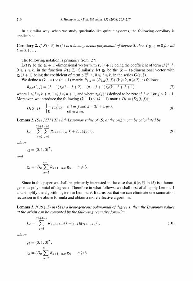
In a similar way, when we study quadratic-like quintic systems, the following corollary isapplicable.

Corollary 2. If R(z, z) in (5) is a homogeneous polynomial of degree 5, then L2k+1 = 0 for allk = 0,1, . . . .

The following notation is primarily from [27].Let rk be the (k + 1)-dimensional vector with rk(j + 1) being the coefficient of term zj zk−j ,

0 � j � k, in the function R(z, z). Similarly, let gk be the (k + 1)-dimensional vector withgk(j + 1) being the coefficient of term zj zk−j , 0 � j � k, in the series G(z, z).

We define a (k + n) × (n + 1) matrix Rk,n = (Rk,n(i, j)) (k � 2, n � 2), as follows:

Rk,n(i, j) = (j − 1)rk(i − j + 2) + (n − j + 1)rk(k − i + j + 1), (7)

where 1 � i � k + n,1 � j � n + 1, and where rk(j) is defined to be zero if j < 1 or j > k + 1.Moreover, we introduce the following (k + 1) × (k + 1) matrix Dk = (Dk(i, j)):

Dk(i, j) ={

− 1k−2i+2 if i = j and k − 2i + 2 �= 0,

0 otherwise.(8)

Lemma 2. (See [27].) The kth Lyapunov value of (5) at the origin can be calculated by

Lk =2k+1∑n=2

n+1∑j=1

R2k+3−n,n(k + 2, j)gn(j), (9)

where

g2 = (0,1,0)T ,

and

gn = iDn

n−1∑m=2

Rn+1−m,mgm, n � 3.

Since in this paper we shall be primarily interested in the case that R(z, z) in (5) is a homo-geneous polynomial of degree s. Therefore in what follows, we shall first of all apply Lemma 1and simplify the algorithm given in Lemma 9. It turns out that we can eliminate one summationrecursion in the above formula and obtain a more effective algorithm.

Lemma 3. If R(z, z) in (5) is a homogeneous polynomial of degree s, then the Lyapunov valuesat the origin can be computed by the following recursive formula:

Lk =2k+4−s∑

j=1

Rs,2k+3−s(k + 2, j)g2k+3−s(j), (10)

where

g2 = (0,1,0)T ,

gn = iDn

n−1∑m=2

Rn+1−m,mgm, n � 3.


Proof. If R(z, z) in (5) is a homogeneous polynomial of degree s, then rk(j) = 0 andRk,n(i, j) = 0 if k �= s. Therefore g2 = (0,1,0)T , gn = 0, for 3 � n � s + 1, and

gn = iDnRs,n+1−sgn+1−s , n � s + 1. (11)

Thus relation (10) follows. �Corollary 3. If s = 4 and, respectively, s = 5, then the Lyapunov values of the system at theorigin can be obtained, by the following formulas:

Lk =2k∑

j=1

R4,2k−1(k + 2, j)g2k−1(j), s = 4, (12)

and, respectively,

Lk =2k−1∑j=1

R5,2k−2(k + 2, j)g2k−2(j), s = 5. (13)

3. An example of quartic system having a fine focus of degree 18

In this section, we shall mainly work on system (5) where R(z, z) is homogeneous polynomialof degree 4. Rewrite the system into the following form:

z = iz + (α1 + iα2)z4 + (α3 + iα4)z

3z + (α5 + iα6)z2z2

+ (α7 + iα8)zz3 + (α9 + iα10)z

4, (14)

where all coefficients αi are real. By computing the Lyapunov constants of the system, we shalllook for systems within such a form which can have as high as possible order of fine focus.

First of all, according to Corollary 1, we know that Lk must be zero if k is not a natural numberdividable by 3. On the other hand, by the algorithm (12) in Corollary 13, we can compute L3straightforwardly:

L3 = −2(α5α4 + α3α6 + α1α8 + α2α7). (15)

Certainly, we have various kinds of possibilities to choose these parameters to let (15) hold.Yet for the moment we want to concentrate on some particular examples under study in this note.We present the following well-chosen set of parameters such that the order of fine focus canreach as high as 18. We tested quite a few other possibilities to produce a higher order of finefocus. On the other hand, we conjecture that the highest possible order of fine focus for quarticsystem is 21, one step away from 18.

Now in (15) we set α1 = α7 = α5 = α6 = 0. Then it follows that L3 = 0. Under these condi-tions, we can proceed the calculation one step further to L6. That is,

L6 = −2

5(α2 + 2α8)

(2α3α10α8 + 4α3α10α2 + 3α2

3α9

− 4α9α4α2 − 3α9α24 − 2α9α4α8 − 6α3α4α10

).

In order to let the relation L6 = 0 stand, we can set α3 = α4 = 0. In fact, with such an assump-tion, automatically, we shall have L9 = 0. Furthermore, we can find


L12 = − 4

525α9(α2 + 2α8)(α2 − 2α8)(4α2 − α8)

× (α2

9 − 3α210

)(59α8 + 30α2)(4α8 + α2).

Clearly, the relation L12 = 0 holds under the sufficiency condition α2 = 2α8. Thus we caneasily move one step further to obtain L15 as follows:

L15 = − 7

320α9α

58

(α2

9 − 3α210

)(52278α2

8 − 20723α29 − 20723α2

10

).

At this stage, if we put α9 = 0, then the origin of the system is a center because in this case thesystem is reversible. Below we assume that α9 �= 0. Therefore, under a scale of the parametersif necessary, we can naturally impose an extra relation α2

9 + α210 = 1. Equivalently, we take

α9 = cos θ , α10 = sin θ . Now in order to make L15 vanish, one can ask a sufficient condition

α8 =√

2072352278 .

Finally we can obtain the following Lyapunov constant L18:

L18 = −189333165503483774277911

381799174273650079066137600

√1083356994α9

(α2

9 − 3α210

).

Therefore if α9 �= 0 and if α29 − 3α2

10 �= 0, then L18 �= 0. This means that indeed there arequartic systems with homogeneous linear terms having a fine focus of degree 18.

If we move some steps further, we see that L21 is already proportional to L18. More exactly,we have

L21 = 189231441601580144758357543795895753

20550504270765144046888759879802880000

√1083356994α9

(α2

9 − 3α210

),

which means that

L21 = −152876554203535967575188481

8233069502645188206033600L18.

In conclusion, if α9 �= 0 and if α29 − 3α2

10 �= 0, then the system

z = iz + 2i

√20723

52278z4 + i

√20723

52278zz3 + (α9 + iα10)z

4

has the fine focus of order 18. We can put this system into the following form under a linear scaleof z and z:

z = iz + 2iz4 + izz3 +√

52278

20723eiθ z4.

Notice that the conditions α9 �= 0 and α29 − 3α2

10 �= 0 can be expressed as follows:

θ �= kπ + π

2, kπ ± π

6, k ∈ Z.

If we go on to find more Lyapunov values, as we have calculated up to L30, all the constantsare proportional to L18. In fact, when θ = kπ ± π

6 , the system is reversible and indeed it hasa center at the origin.2

2 We thank J. Giné for pointing out the reversibility of the system in this case.


4. An example of quintic system having a fine focus of degree 18

This section is devoted to finding an example of quintic system having a fine focus of de-gree 18. That is, we consider system (5), where R(z, z) is a homogeneous polynomial of degree 5,with the following explicit form:

z = iz + (α1 + iα2)z5 + (α3 + iα4)z

4z + (α5 + iα6)z3z2

+ (α7 + iα8)z2z3 + (α9 + iα10)zz

4 + (α11 + iα12)z5, (16)

where all αi are real constants.We shall use the same algorithm as adopted in the last section for quartic system. Although

the example we shall present has the same degree of fine focus like in the quartic case, we feelthat this order is the maximally possible one for quadratic-like quintic systems.

To calculate the Lyapunov constants of system (16), it suffices only to consider L2l , for l =1,2, . . . . This is because, by Corollary 1, one always has L2l+1 = 0.

By the formula (13), some straightforward computation gives

L2 = 2α5.

Thus we have only one possibility to take α5, i.e., α5 = 0.Now by putting α5 = 0, we can proceed the calculation to L4. Namely, we have

L4 = −2(α9α2 + α1α10 + α7α4 + α3α8).

To let this relation hold, we have different ways to fix the parameters. Again, like in the quarticcase, after certain attempts, we take the following particular set of parameters:

α7 = α8 = α2 = α10 = 0.

Consequently, we arrive at the following stage:

L6 = 2

3(α3α11 − α4α12)(−α1 + 3α9).

There are two factors in the expression of L6. Here we can simply assume that α1 = 3α9 to moveone step further:

L8 = 8α12α9α6α4 + 1

3α11α

34 + α12α3α

24 + 4α12α3α

29

− 4α11α4α29 − α11α

23α4 − 1

3α12α

33 − 8α11α6α3α9. (17)

In expression (17), we can put α12 = α6 = α4 = 0 to make the relation L8 = 0 hold. Conse-quently, we obtain the following relations:

L10 = −16α3α29 − 16

3α2

9α11 + 12

5α3α

211 − 4α3

3, (18)

L12 = 0,

and

L14 = 134α53 + 9856

9α3

3α29 − 128

35α2

3α311 + 6464

3α3α

49 − 478

105α3α

411

− 11968

45α2

9α3α211 − 4

15α4

3α11 + 3776

15α2

3α11α29 − 24292

315α3

3α211

+ 416α2

9α311 + 11456

α49α11. (19)

135 15


Without imposing any further restrictions, we can compute another two Lyapunov constants,L16 and L18. They are given by

L16 = 0,

and

L18 = 1087

54α3α

611 + 368357

756α4

3α311 + 4439

1260α2

3α511 − 204790

3α5

3α29

+ 21643673

14175α2

9α3α411 + 8471860

189α2

11α3α49 − 12581

2α7

3

− 1311328

9α6

9α11 − 134963

315α11α

63 − 4075753

315α11α

43α2

9

− 66195484

945α11α

23α4

9 − 820984

3α3

3α49 + 4488437

1260α5

3α211

+ 54464521

2835α2

11α33α2

9 − 430048

189α4

9α311 − 67904

8505α2

9α511

+ 413419

1620α3

3α411 − 405024α6

9α3 − 371723

945α2

3α311α

29 . (20)

Below it suffices to prove the existence of solutions, in terms of the parameters α’s, of thesystem of algebraic equations

L10 = 0, L14 = 0, L18 �= 0.

To this end, we assume that α9 = β1α3, α11 = β2α3, and substitute them into the above expres-sions (18), (19) and (20). We have

L10 = 4

15

(9β2

2 − 60β21 − 20β2β

21 − 15

)α5

3β1β2,

L14 =(

134 − 4

15β2 − 24292

315β2

2 − 128

35β3

2 − 478

105β4

2

+ 9856

9β2

1 + 3776

15β2

1β2 − 11968

45β2

1β22 + 416

135β2

1β32

+ 6464

3β4

1 + 11456

15β4

1β2

)α7

3β1β2,

and

L18 =(

−12581

2− 134963

315β2 + 4488437

1260β2

2 + 368357

756β3

2 + 413419

1620β4

2

+ 4439

1260β5

2 + 1087

54β6

2 − 204790

3β2

1 − 4075753

315β2

1β2

+ 54464521

2835β2

1β22 − 371723

945β2

1β32 + 21643673

14175β2

1β42

− 67904

8505β2

1β52 − 820984

3β4

1 − 66195484

945β4

1β2 + 8471860

189β4

1β22

− 430048β4

1β32 − 405024β6

1 − 1311328β6

1β2

)α9

3β1β2.
189 9


If we take β2 ∈ (−3,−√5/3) and

β21 = 3

20

(3β22 − 5)

(β2 + 3), (21)

then it follows that

9β22 − 60β2

1 − 20β2β21 − 15 = 0.

Consequently, L10 = 0. Moreover, by substituting the relation (21) into L14 and L18, we have

L14 = − 2α73β1β2

2625(β2 + 3)2F(β2),

L18 = α73β1β

22

47250(β2 + 3)3G(β2),

where

F(β2) = 4155β62 − 10716β5

2 − 63285β42 − 18070β3

2

+ 168075β22 + 205450β2 + 60375,

and

G(β2) = 781365β82 + 18402357β7

2 − 39352164β62

− 295090087β52 − 206364414β4

2 + 680783545β32

+ 1213555470β22 + 666947025β2 + 115223175.

The possibility to take β2 ∈ (−3,−√5/3) can be verified from the observation that F(−3) =

1951488 > 0, and F(−3/2) < −322 < 0. This means that indeed there exists β0 ∈ (−3,−√5/3)

such that F(β0) = 0. Since F(x) and G(x) have no common factors, therefore G(β0) �= 0 andconsequently L18 �= 0. Moreover, because

3

20

(3β20 − 5)

(β0 + 3)> 0,

it follows that if we take

α2 = α4 = α5 = α6 = α7 = α8 = α10 = α12 = 0,

and

α3 = ∓√

20

3

(β0 + 3)

(3β20 − 5)

, α1 = 3, α9 = 1, α11 = β0α3,

where β0 is the root of F(β) = 0 in (−3,−√5/3), then

Lk = 0, k = 1, . . . ,17, L18 �= 0.

That means that the following system has the fine focus of degree 18.

E5: z = iz + 3z5 +√

20(β0 + 3)

9β20 − 15

z4z + zz4 +√

20(β0 + 3)β20

9β20 − 15

z5. (22)

Notice that system (22) contains no parameter.


References

[1] A.A. Andronov, E.A. Leontovich, I.I. Gordon, A.G. Maier, Theory of Bifurcations of Dynamical Systems ona Plane, John Wiley, New York, 1973.

[2] J. Bai, Y. Liu, A class of planar degree n (even number) polynomial systems with a fine focus of order n2 − n,Chinese Sci. Bull. 12 (1992) 1063–1065.

[3] N.N. Bautin, On the number of limit cycles which appear with the variation of coefficients from an equilibriumposition of focus or center type, Mat. Sb. 30 (1952) 181–196; English transl. in: Math. USSR-SB 100 (1954) 397–413.

[4] M. Caubergh, F. Dumortier, Hopf–Takens bifurcations and centres, J. Differential Equations 202 (2004) 1–31.[5] J. Chavarriga, J. Giné, Integrability of a linear center perturbed by fourth degree homogeneous polynomial, Publ.

Mat. 40 (1996) 21–39.[6] J. Chavarriga, J. Giné, Integrability of a linear center perturbed by fifth degree homogeneous polynomial, Publ.

Mat. 41 (1997) 335–356.[7] C.S. Coleman, Hilbert’s 16th problem: How many cycles? in: Differential Equation Models, Modules in Applied

Mathematics, vol. 1, Springer-Verlag, New York, pp. 279–297.[8] W.A. Coppel, A survey of quadratic systems, J. Differential Equations 2 (1966) 293–304.[9] H. Dulac, Détermination et intégration d’une certaine classe d’équations différentielle ayant pour point singulier un

centre, Bull. Sci. Math. Sér. (2) 32 (1908) 230–252.[10] J.P. Françoise, Successive derivatives of a first return map, application to the study of quadratic vector fields, Ergodic

Theory Dynam. Syst. 16 (1996) 87–96.[11] M. Frommer, Über das Auftreten vem Wirbeln und Strudeln (geschlossener und spiralieger Integralkurven) in der

Umbegung rationaler Unbestimmtheitsstellen, Math. Ann. 109 (1933/1934) 395–424.[12] F. Gobber, K.D. Willamowskii, Lyapunov approach to multiple Hopf bifurcation, J. Math. Anal. Appl. 71 (1979)

333–350.[13] Yu.S. Ilyashenko, Finiteness for Limit Cycles, Transl. Math. Monographs, vol. 94, Amer. Math. Soc., Providence,

RI, 1991.[14] W. Kapteyn, On the midpoints of integral curves of differential equations of the first degree, Nederl. Akad. Weten-

sch. Verslag Afd. Natuurk. 20 (1912) 1354–1365.[15] W. Li, Theory and Applications of Normal Forms, Science Press, Beijing, 2000.[16] J. Li, Hilbert’s 16th problem and bifurcations of planar polynomial vector fields, Int. J. Bifurcation and Chaos 13

(2003) 47–106.[17] J. Llibre, Integrability of polynomial differential systems, in: Handbook of Differential Equations (Ordinary Differ-

ential Equations, vol. 1), Elsevier, North-Holland, Amsterdam, pp. 437–532.[18] N.G. Lloyd, Limit cycles of polynomial systems, some recent developments, in: T. Bedford, J. Swift (Eds.), New

Directions in Dynamical Systems, Lecture Notes, vol. 127, London Mathematical Soc., pp. 192–234..[19] N.G. Lloyd, J.M. Pearson, Conditions for a centre and the bifurcation of limit cycles in a class of cubic systems, in:

Lecture Notes in Mathematics, vol. 1455, pp. 231–242.[20] N.G. Lloyd, C.J. Christopher, J. Devlin, J.M. Pearson, N. Yasmin, Quadratic-like cubic systems, Differential Equa-

tions Dynam. Syst. 5 (1997) 329–345.[21] M.A. Lyapunov, Problème Général de la Stabilité de Mouvement, Princeton Univ. Press, Princeton, NJ, 1947 (First

printing, 1892, Harkov).[22] H. Poincaré, Mémoire sur les courbes définies par les équations différentielles, J. Math. Pures Appl. 1 (1885) 167–

244; Oeuvres de Henri Poincaré, vol. 1, Gauthier-Villars, Paris, pp. 95–114.[23] D. Schlomiuk, Algebraic and geometric aspects of the theory of polynomial vector fields, in: D. Schlomiuk (Ed.),

Bifurcations and Periodic Orbits of Vector Fields, NATO SAI Series C, vol. 408, Kluwer Academic, London,pp. 429–467.

[24] S. Shi, On the structure of Poincaré–Lyapunov constants for the weak focus of polynomial vector fields, J. Differ-ential Equations 52 (1984) 52–57.

[25] K.S. Sibirskii, The number of limit cycles in the neighborhood of a singular point, Differential Equations 1 (1965)36–47.

[26] D. Wang, A recursive formula and its applications to computations of normal forms and focal values in dynamicalsystems, in: S. Liao, T. Ding, Y. Ye (Eds.), Nankai Series in Pure, Applied Mathematics and Theoretical Physics,vol. 4, World Scientific Publishing Co. Pte. Ltd., Singapore, pp. 238–247.

[27] D. Wang, R. Mao, A complex algorithm for computing Lyapunov values, Random and Computational Dynamics 2(1994) 261–277.


[28] Y. Ye, et al., The Theory of Limit Cycles, Transl. Math. Monographs, vol. 66, Amer. Math. Soc., Providence, RI,1984.

[29] Y. Ye, Qualitative Theory of Polynomial Differential Systems, Shanghai Scientific and Technical Publishers, Shang-hai, 1995.

a quartic system and a quintic system with fine focus of order 18

Documents