a queueing model for mixed loss-delay systems with general interarrival processes for wide-band...

European Journal of Operational Research 180 (2007) 1201–1220

www.elsevier.com/locate/ejor

Stochastics and Statistics

A queueing model for mixed loss-delay systems with generalinterarrival processes for wide-band calls

Ming Fan *

Institute of Mathematics, Natural Sciences and Engineering, Dalarna University, 781 88 Borlange, Sweden

Received 19 April 2005; accepted 26 May 2006Available online 5 September 2006

Abstract

We investigate the single link mixed loss-delay FIFO system with the exponential holding time distribution, the Mar-kovian interarrival process for the narrow-band calls, and the general independently and identically distributed interarrivalprocess for the wide-band calls. This is achieved by combining the embedded Markov chain method and the matrix-ana-lytic technique.� 2006 Elsevier B.V. All rights reserved.

Keywords: Embedded Markov chain; Matrix-geometric solution; Mixed loss-delay system; Waiting room

1. Introduction and basic assumptions

The traditional call traffic model for network services, such as telephony, FTP transfers, and telnet sessions,is based on Poisson call arrivals and exponentially distributed call holding times. However, for the WorldWide Web (WWW) service which contributes to a large portion of the TCP traffic in the internet, the Poissonmodel is inadequate. Recent measurements indicate that TCP connection arrivals in the internet have self-sim-ilar behaviour, which exhibits structural similarities across a wide range of time scales. Measurements havealso shown that the call holding time distribution of the WWW service is more heavy tailed than the exponen-tial distribution [2].

The present paper deals with the queueing model of a single link mixed loss-delay FIFO system. A com-munication link is assumed to be offered two types of traffic: a narrow-band (NB) traffic type subject tothe loss model and a wide-band (WB) traffic type subject to the delay model. In 1988, De Serres and Masonstudied the traditional multi-server queue with the exponential holding time distribution and the Markovianinterarrival process [1]. One of their two approaches but more effective is to use the matrix-analytic techniquedue to Neuts [5]. We will focus on the single link mixed loss-delay system with the exponential holding timedistribution, the Markovian interarrival process for the narrow-band calls, and the general independently and

0377-2217/$ - see front matter � 2006 Elsevier B.V. All rights reserved.

doi:10.1016/j.ejor.2006.05.021

* Tel.: +46 23778853.E-mail address: [email protected]

mailto:[email protected]

1202 M. Fan / European Journal of Operational Research 180 (2007) 1201–1220

identically distributed renewal arrival process for the wide-band calls. The main idea is to combine the embed-ded Markov chain method and the matrix-analytic technique, and apply them on the queueing model studiesin the multi-service systems.

Assume the following:

• one narrow-band (NB) class subject to loss when the link is busy with the bandwidth unit bn = 1,• one wide-band (WB) class subject to delay when the link is busy with the bandwidth units bw > 1,• C servers, where C = rbw + s with 0 6 s < bw,• a finite or infinite waiting room,• cut-off factor r0, the maximal number of WB calls that can be in service simultaneously,• the call arrival process of NB class with a Markovian interarrival time distribution F1ðtÞ ¼ 1� e�k1t and

the mean arrival rate k1 ¼ 1=EfF1g,• the call arrival process of WB class with a general independent interarrival time distribution F2ðtÞ and the

mean arrival rate k2 ¼ 1=EfF2g,• the call holding time of NB class with an independent exponential distribution G1ðtÞ ¼ 1� e�l1t and the

mean departure rate l1 ¼ 1=EfG1g,• the call holding time of WB class with an independent exponential distribution G2ðtÞ ¼ 1� e�l2t and the

mean departure rate l2 ¼ 1=EfG2g,• load q ¼ k2

r0l2< 1.

Observe that, in this mixed loss-delay system, the bandwidth factor bw/C reserves a number of channels forthe NB traffic, while the cut-off factor r0 protects the NB traffic against overload of the WB traffic. Let nowX(t) and Y(t) be the numbers of NB and WB calls, respectively, in the system at epoch t, with the states (i, j) forwhich 0 6 i 6 C and j P 0. Define the following stationary distributions in the system with an infinite waitingroom:

• p(i, j) = the long-run fraction of calls who find upon arrival i other NB calls and j other WB calls present inthe system,

• p(i, j) = the long-run fraction of time that i NB calls and j WB calls are present in the system.

Let us introduce now the steady-state probability vectors by

~pðjÞ ¼ ðpð0; jÞ; pð1; jÞ; . . . ; pðC; jÞÞ;~pðjÞ ¼ ðpð0; jÞ; pð1; jÞ; . . . ; pðC; jÞÞ;

for j P 0, and let

~p ¼ ð~pð0Þ;~pð1Þ; . . . ;~pðjÞ; . . .Þ;~p ¼ ð~pð0Þ;~pð1Þ; . . . ;~pðjÞ; . . .Þ:

For~x ¼ ðx0; . . . ; xCÞ 2 RCþ1, the l1-norm of~x is given by

k~xk1 ¼XC

i¼0

jxij:

If~x ¼ ð~xð0Þ; . . . ;~xðjÞ; . . .Þ, for which~xðjÞ 2 RCþ1, j P 0, and
XjP0
k~xðjÞk1 <1;

we denote the l1-norm of~x by

k~xk1 ¼XjP0

k~xðjÞk1:

M. Fan / European Journal of Operational Research 180 (2007) 1201–1220 1203

For a C + 1 by C + 1 matrix A = (ami)06m, i6C, we consider its norm kAk and spectral radius sp(A) by

kAk ¼ max06m6C

XC

i¼0

jamij( )

¼ supfkA~xk1j~x 2 RCþ1; k~xk1 6 1g ð1:1Þ

and

spðAÞ ¼ maxfjnjjn is an eigenvalue of Ag;
respectively. It is known that
spðAÞ ¼ limk!1kAkk1=k

: ð1:2Þ

Moreover, for a, b P 0, we denote a _ b ¼ maxfa; bg; a ^ b ¼ minfa; bg, and denote [a] to be the largest inte-ger 6a.

This paper is organized as follows. In Section 2, we introduce the two-dimensional embedded Markovchain model for the above mentioned mixed loss-delay system, and formulate the transition rate matrix asa block-partitioned GI/M/r0 type Markov chain in the sense of [5, Chapter 1]. In Section 3, the ergodicity the-orem and the matrix-geometric solutions for the arrival stationary distribution~p at the embedded epoches arepresented. In Section 4, the recursive solutions for the time stationary distribution~p at an arbitrary time epochare given in terms of the birth–death equations, and the performance measures of the system are determined.Section 5 provides a comparison between systems with finite or infinite waiting rooms. We conclude the paperin Section 6 by a summary and some remarks concerning the forthcoming research.

2. Two-dimensional embedded Markov chain model and transition rate matrix

With the basic assumptions given in Section 1, a two-dimensional embedded Markov chain model can bedefined at WB call arrival instants. Let tn be the arrival instant of the nth WB call, and let Xn = X(tn � 0) andYn = Y(tn � 0) be the numbers of NB calls (in service only) and WB calls (in service or queue), respectively,found upon the arrival of the nth WB call. Then (Xn,Yn) is a two-dimensional embedded Markov chain withthe state space

X ¼ fði; jÞj0 6 i 6 C; j P 0g;
where the states are ordered lexicographically as below
ð0; 0Þ; ð1; 0Þ; . . . ; ðC; 0Þ; ð0; 1Þ; ð1; 1Þ; . . . ; ðC; 1Þ; . . .

For j P 0, the set of states {(0, j), (1, j), . . . , (C, j)} is called the level j.For k, j P 0 and 0 6 m, i 6 C, let p(m,k)(i,j) be the one step transition probability from the state (m,k) to the

state (i, j), which is independent of n, in the following way:

pðm;kÞði;jÞ ¼ PrfðX nþ1; Y nþ1Þ ¼ ði; jÞjðX n; Y nÞ ¼ ðm; kÞg:

Thus, the Markov chain (Xn,Yn) is homogeneous. With tn+1 � tn as the interarrival time between the nth andthe (n + 1)th WB calls, we denote

qmiðt; jÞ ¼ PrfX nþ1 ¼ ijX n ¼ m; Y nþ1 ¼ j; t ¼ tnþ1 � tng:
Now we turn to specify the transition probabilities p(m,k)(i,j).
• In case 0 6 m 6 C � r0bw and 0 6 i 6 C � ðj ^ r0Þbw:

qmiðt; jÞ ¼Xm1

m¼m0

mþ m

i

� �ðk1tÞm

m!ð1� e�l1tÞmþm�ie�ðk1þil1Þt

þX1

m¼m1þ1

mþ m1

i

� �ðk1tÞm

m!ð1� e�l1tÞmþm1�ie�ðk1þil1Þt; ð2:1Þ

where m0 ¼ ði� mÞ _ 0 and m1 ¼ C � m� ðj ^ r0Þbw.


If j 6 k + 1 6 r0, then

pðm;kÞði;jÞ ¼Z 1

0

k þ 1

j

� �ð1� e�l2tÞkþ1�je�jl2tqmiðt; jÞdF2ðtÞ: ð2:2Þ

If r0 6 j 6 k + 1, then


0

ðr0l2tÞkþ1�j

ðk þ 1� jÞ! e�r0l2tqmiðt; jÞdF2ðtÞ: ð2:3Þ

If j < r0 < k + 1, then


0

r0

j

� �e�jl2t

Z t

0

ðr0l2sÞk�r0

ðk � r0Þ!ðe�l2s � e�l2tÞr0�jr0l2 ds

!qmiðt; jÞdF2ðtÞ: ð2:4Þ

• In case sþ ðl� 1Þbw þ 1 6 m 6 sþ lbw and 0 6 i 6 C � ðj ^ ðr � lÞÞbw with r � r0 þ 1 6 l 6 r:

qmiðt; jÞ ¼Xm1

m¼m0

mþ m

i

� �ðk1tÞm

m!ð1� e�l1tÞmþm�ie�ðk1þil1Þt þ

X1m¼m1þ1

mþ m1

i

� �ðk1tÞm

m!ð1� e�l1tÞmþm1�ie�ðk1þil1Þt;

ð2:5Þ
where m0 ¼ ði� mÞ _ 0 and m1 ¼ C � m� ðj ^ ðr � lÞÞbw.If j 6 k + 1 6 r � l, then

0

k þ 1

j

� �ð1� e�l2tÞkþ1�je�jl2tqmiðt; jÞdF2ðtÞ: ð2:6Þ

If r � l 6 j 6 k + 1, then


0

ððr � lÞl2tÞkþ1�j

ðk þ 1� jÞ! e�ðr�lÞl2tqmiðt; jÞdF2ðtÞ: ð2:7Þ

If j < r � l < k + 1, then


0

r � l

j

� �e�jl2t

Z t

0

ððr � lÞl2sÞk�rþl

ðk � r þ lÞ! ðe�l2s � e�l2tÞr�l�jðr � lÞl2 ds

!qmiðt; jÞdF2ðtÞ:

ð2:8Þ
In particular, if C � bw + 1 6 m 6 C and 0 6 i 6 C, then
pðm;kÞði;kþ1Þ ¼Z 1

0

qmiðt; jÞdF2ðtÞ: ð2:9Þ

• In the other case:

pðm;kÞði;jÞ ¼ 0: ð2:10Þ

In fact, (2.2) and (2.6) follow from (2.1), (2.5) and [4, (6.9)], for which no WB calls are waiting and all presentare engaged with their own server prior to the arrival of the (n + 1)th WB call; (2.3) and (2.7) follow from(2.1), (2.5) and [4, (6.10)], for which all available servers for WB calls are busy throughout the interarrival per-iod prior to the arrival of the (n + 1)th WB call; and (2.4) and (2.8) follow from (2.1), (2.5) and [4, (6.13)], forwhich some WB calls are in service while other WB calls are waiting in queue prior to the arrival of the(n + 1)th WB call.

Let us place all of these one-step transition probabilities in the following matrix which is represented inblock-partitioned form as

P ¼ ðP kjÞk;jP0;

where Pkj = (p(m,k)(i,j))06m,i6C are C + 1 by C + 1 matrices.


Theorem 2.1. Let P = (Pkj) be the matrix given above.

(i) The first (C � bw) rows of Pk0 consist of positive entries; in each row and column of Pk,k+1, there exists at

least one positive entry; Pkj = 0 for k + 1 < j.(ii) P is stochastic, namely, for fixed m and k,
X
jP0

XC

i¼0

pðm;kÞði;jÞ ¼ 1:

(iii) Pkj = Pk+1,j+1 for k + 1 P j P r0.

(iv) If j P r0 � 1, then

XC

i¼0

Xj

l¼0

pðm;kÞði;lÞ PXC

i¼0

Xj

l¼0

pðm;kþ1Þði;lÞ:

Proof. Part (i) follows directly from (2.1) to (2.10). By (2.1) and (2.5), we have

Xmþm1

i¼0

qmiðt; jÞ ¼Xm1

m¼0

Xmþm

i¼0

mþ m

i

!ðk1tÞm

m!ð1� e�l1tÞmþm�ie�ðk1þil1Þt

þX1

m¼m1þ1

Xmþm1

i¼0

mþ m1

i

!ðk1tÞm

m!ð1� e�l1tÞmþm1�ie�ðk1þil1Þt

¼X1m¼0

ðk1tÞm

m!e�k1t ¼ 1:

Part (ii) can be obtained now by calculation as in [4, Chapter 6]. For part (iii), if k + 1 P j P r0 andr � r0 + 1 6 l 6 r, then k P j � 1 P r0 � 1 P r � l. Together with (2.3), (2.7) and the equality (k + 1) +1 � (j + 1) = k + 1 � j, we have

pðm;kÞði;jÞ ¼ pðm;kþ1Þði;jþ1Þ; ð2:11Þ

and hence Pkj = Pk+1,j+1 for k + 1 P j P r0. We turn now to part (iv). If k + 1 < j, then

XC

i¼0

Xj

l¼0

pðm;kÞði;lÞ ¼Xkþ1

l¼0

XC

i¼0

pðm;kÞði;lÞ ¼ 1 PXC

i¼0

Xj

l¼0

pðm;kþ1Þði;lÞ:

If k + 1 P j P r0 � 1, then

XC

i¼0

Xj

l¼0

pðm;kÞði;lÞ ¼ 1�Xkþ1

l¼jþ1

XC

i¼0

pðm;kÞði;lÞ

and

XC

i¼0

Xj

l¼0

pðm;kþ1Þði;lÞ ¼ 1�Xkþ2

l¼jþ1

XC

i¼0

pðm;kþ1Þði;lÞ ¼ 1�Xkþ1

l¼j

XC

i¼0

pðm;kÞði;lÞ

by (2.11). This implies the estimate in (iv). h

Let Ak ¼ P k;r0for k P r0 � 1. Now we can write the transition rate matrix P of the Markov chain (Xn,Yn) as

below:


P ¼

P 00 P 01

P 10 P 11 P 12 0

..

. . .. . .

. . ..

P r0�1;0. .

. . ..

P r0�1;r0�1 Ar0�1

P r0;0. .

. . ..

P r0;r0�1 Ar0Ar0�1

P r0þ1;0. .

. . ..

P r0þ1;r0�1 Ar0þ1 Ar0

. ..

..

. . .. . .

. . .. . .

. . .. . .

.

0BBBBBBBBBBBBBBBB@

1CCCCCCCCCCCCCCCCA: ð2:12Þ

This model is formulated for the loss-delay system with an infinite waiting room. In real life, however, oneusually consider the system with a finite waiting room of size K including servers. In that case, the systemcan be modeled as a finite two-dimensional embedded Markov chain ðX n; Y ðKÞn Þ with the state space

XðKÞ ¼ ði; jÞj0 6 i 6 C; 0 6 iþ jbw 6 K; j ¼ j0 þ j00 with j0 6C � i

bw

� �^ r0 and j00 P 0

� �:

Observe that if (m,k) 2 X(K) with k P 1, then (m,k � 1) 2 X(K). Thus, for (m,k), (i, j) 2 X(K), we have

pðKÞðm;kÞði;jÞ ¼ pðm;kÞði;jÞ if k <K � m

bw

� �
and
pðKÞðm;kÞði;jÞ ¼ pðm;k�1Þði;jÞ if k ¼ K � mbw

� �:

It is clear that, if k < K�mbw

h i, then
XC
i¼0

Xj

l¼0

pðKÞðm;kÞði;lÞ ¼XC

i¼0

Xj

l¼0

pðm;kÞði;lÞ: ð2:13Þ

Furthermore, if k ¼ K�mbw

h iand j P r0 � 1, then
XC
i¼0

Xj

l¼0

pðKÞðm;kÞði;lÞ PXC

i¼0

Xj

l¼0

pðm;kÞði;lÞ ð2:14Þ

by Theorem 2.1(iv). For (i, j) 2 X(K), we denote by p(K)(i, j) and p(K)(i, j) the corresponding steady-state prob-abilities. For simplicity, we may define

pðKÞði; jÞ ¼ pðKÞði; jÞ ¼ 0

for 0 6 i 6 C, 0 6 j 6 [K/bw] but (i, j) 62 X(K). Thus, the corresponding stationary distributions are given by

~pðKÞðjÞ ¼ ðpðKÞð0; jÞ; . . . ; pðKÞðC; jÞÞ; ~pðKÞðjÞ ¼ ðpðKÞð0; jÞ; . . . ; pðKÞðC; jÞÞ
for 0 6 j 6 [K/bw], and
~pðKÞ ¼ ð~pðKÞð0Þ; . . . ;~pðKÞð½K=bw�ÞÞ; ~pðKÞ ¼ ð~pðKÞð0Þ; . . . ;~pðKÞð½K=bw�ÞÞ:

3. Matrix-geometric solutions for the arrival stationary distribution

The transition rate matrix P in (2.12) determines a GI/M/r0 type Markov chain (Xn,Yn) with complexboundary behaviour in the sense of [5, Chapter 1], which is a natural generalization of the one-dimensionalmodel given in [3] or [4, Chapter 6]. Here each entry in the transition matrix is replaced with a C + 1 byC + 1 submatrix. It is easy to see that the Markov chain (Xn,Yn) is irreducible by Theorem 2.1(i) and induc-tion. In this section, we investigate the arrival stationary distribution


pði; jÞ ¼ limn!1

PrfðX n; Y nÞ ¼ ði; jÞg ð3:1Þ

for 0 6 i 6 C and j P 0.Let

A ¼X

kPr0�1

Ak: ð3:2Þ

By (2.3) and (2.7),
XkPr0�1
pðm;kÞði;r0Þ ¼Z 1

0

qmiðt; r0ÞdF2ðtÞ:

Thus,

A ¼ ðamiÞ06m;i6C;

where

ami ¼Z 1

0

qmiðt; r0ÞdF2ðtÞ

for 0 6 m 6 C � r0bw and 0 6 i 6 C � r0bw, or s + (l � 1)bw + 1 6 m 6 s + lbw and 0 6 i 6 C � (r � l)bw withr � r0 + 1 6 l 6 r; and ami = 0 otherwise. Thus, A is a stochastic matrix. Furthermore, let R be the minimalnonnegative solution of the matrix equation

R ¼X

kPr0�1

Rk�r0þ1Ak; ð3:3Þ

and let B[R] be the stochastic matrix given by

B½R� ¼

P 00 P 01 0

P 10 P 11 P 12

..

. ... ..

. . ..

P r0�2;0 P r0�2;1 P r0�2;2 . . . P r0�2;r0�1

B0½R� B1½R� B2½R� . . . Br0�1½R�

0BBBBBBB@

1CCCCCCCA; ð3:4Þ

where

Bj½R� ¼X

kPr0�1

Rk�r0þ1P kj for 0 6 j 6 r0 � 1:

Theorem 3.1. Let P be the transition rate matrix given in (2.12), and let R be the matrix given in (3.3).

(i) The eigenvalues of the matrix R lie inside the unit disk, and the eigenvalue with largest modulus is real and

positive. Consequently, (IC+1 � R)�1 exists, for which

ðICþ1 � RÞ�1 ¼XkP0

Rk:

(ii) The matrix P is positive recurrent.

Proof. We observe first that the eigenvalue of R with largest modulus is real and positive since P is irreducible.Let X = Aj (j P r0 � 1), A or R. By (2.3) and (2.7), X has the block-partitioned lower triangular form with thediagonal blocks Xll for 0 6 l 6 r0, where X00 is a C � r0bw + 1 by C � r0bw + 1 submatrix, and Xll (1 6 l 6 r0)are bw by bw submatrices. In addition, all All (0 6 l 6 r0) are irreducible, A00 is stochastic, and All are substo-chastic for 1 6 l 6 r0. Thus, sp(A00) = 1, while sp (All) < 1 for 1 6 l 6 r0. We claim

spðRÞ ¼ max06l6r0

spðRllÞ < 1:


By (3.3), Rll is the minimal nonnegative solution of the matrix equation

Rll ¼X

kPr0�1

ðRllÞk�r0þ1ðAkÞll;

and hence sp(Rll) 6 sp(All) for 0 6 l 6 r0 by [5, Lemma 1.3.1]. This implies that sp(Rll) < 1 for 1 6 l 6 r0. Forl = 0, we may apply the similar argument as in [5, Section 1.3] on the irreducible stochastic matrix A00. Let~e ¼ ð1; 1; . . . ; 1; . . .Þ, the row vector in R1 with all components equal to 1, and let

~ek ¼ ð1; 1; . . . ; 1|fflfflfflfflfflffl{zfflfflfflfflfflffl}k

; 0; 0; . . .Þ ¼ ð1; 1; . . . ; 1|fflfflfflfflfflffl{zfflfflfflfflfflffl}k

Þ

for k P 1. For k0 = C � r0bw + 1, we consider now the positive vectors ~a;~b 2 Rk0 given by

~aA00 ¼~a; ~a �~eTk0¼ 1;

and

~bT ¼X

kPr0�1

ðk þ 1� r0ÞðAkÞ00~eTk0:

By (2.3), we have
XC
i¼0

XkPr0�1

ðk þ 1� r0Þpðm;kÞði;r0Þ ¼ r0l2EfF2g ¼1

q

for 0 6 m 6 C � r0bw, which implies that ~b ¼ 1q~ek0

and hence

~a �~bT ¼ 1

q~a �~eT

k0¼ 1

q> 1:

By [5, Lemmas 1.3.4 and 1.3.5], sp(R00) < 1 and hence sp(R) < 1. Observe that B[R] is irreducible by Theorem2.1(i). By a slight modification on the proof of [5, Theorem 1.3.2], we can show that the transition matrix P ispositive recurrent. h

By combining Theorem 3.1 and [5, Theorems 1.2.1 and 1.5.1], we obtain

Theorem 3.2. The equilibrium probabilities given in (3.1) exist and are uniquely determined by

~p ¼~pP and ~p �~eT ¼ 1:

(i) If j P r0, then

~pðjÞ ¼X

kPj�1

~pðkÞAk�jþr0:

(ii) If j P r0 � 1, then ~pðjþ 1Þ ¼~pðjÞR, and hence ~pðjÞ ¼~pðr0 � 1ÞRj�r0þ1.

(iii) The vectors ~pðjÞ, 0 6 r0 � 1, are determined by

ð~pð0Þ; . . . ;~pðr0 � 1ÞÞB½R� ¼ ð~pð0Þ; . . . ;~pðr0 � 1ÞÞ
and
ð~pð0Þ; . . . ;~pðr0 � 2ÞÞ~eTCþ1 þ~pðr0 � 1ÞðICþ1 � RÞ�1~eT

Cþ1 ¼ 1:

The matrix R is called the rate matrix of the system, and the vectors ~pðjÞ, j P r0, are called the modified ma-trix-geometric probability vectors in the sense of [5, Section 1.5]. By [5, Theorem 1.2.3], the rate matrix R sat-isfies the conservation law:

Ar0�1 ¼XkPr0

Rk�r0þ1X

mPkþ1

Am~eTCþ1:

This identity serves as an internal accuracy check on the computation of R.


For illustrative example we consider the case where C = 3, bw = 2, r0 = 1, k1 = 0.7, l1 = 1, l2 = 0.5, and thestopping threshold e = 10�3. We assume that the WB calls have Weibull interarrival time distribution

F2ðtÞ ¼ 1� e�ffiffiffiffiffi0:8tp

;

which implies that

F02ðtÞ ¼

0:4ffiffiffiffiffiffiffiffi0:8tp e�

ffiffiffiffiffi0:8tp

and k2 ¼ 1=EfF2g ¼ 0:4:

Let us determine first the 4 by 4 matrices

Bk ¼ P k0 ¼ ðpðm;kÞði;0ÞÞ06m;i63 and Ak ¼ P k1 ¼ ðpðm;kÞði;1ÞÞ06m;i63

for k P 0. Observe that, for j = 0,1 and 0 6 m 6 3 � j,

qmiðt; jÞ ¼X3�m�2j

m¼ði�mÞ_0

mþ m

i

� �ð0:7tÞm

m!ð1� e�tÞmþm�ie�ð0:7þiÞt

þX1

m¼4�m�2j

3� 2j

i

� �ð0:7tÞm

m!ð1� e�tÞ3�2j�ie�ð0:7þiÞt

in (2.1). Now we have

pðm;0Þði;0Þ ¼ 0:4

Z 1

0

ð1� e�0:5tÞe�ffiffiffiffiffi0:8tp

qmiðt; 0Þdtffiffiffiffiffiffiffiffi0:8tp ;

pðm;kÞði;0Þ ¼ 0:4

Z 1

0

Z t

0

ð0:5sÞk�1

ðk � 1Þ! ðe�0:5s � e�0:5tÞds

!e�ffiffiffiffiffi0:8tp

qmiðt; 0Þdtffiffiffiffiffiffiffiffi0:8tp ;

pðm;0Þði;1Þ ¼ 0:4

Z 1

0

e�ð0:5tþffiffiffiffiffi0:8tp

Þqmiðt; 1Þdtffiffiffiffiffiffiffiffi0:8tp

pðm;kÞði;1Þ ¼ 0:4

Z 1

0

ð0:5tÞk

k!e�ð0:5tþ

ffiffiffiffiffi0:8tp

Þqmiðt; 1Þdtffiffiffiffiffiffiffiffi0:8tp

for m = 0,1 and k P 1 by (2.2)–(2.4); and p(m,k)(i,0) = 0 otherwise. We obtain the matrices given in (3.2)–(3.4)as follows:

A ¼

0:919 0:081 0 0

0:490 0:510 0 0

0:361 0:204 0:408 0:027

0:336 0:147 0:167 0:350

0BBBB@1CCCCA;

R ¼

0:842 0:082 0 0

0:436 0:487 0 0

0:766 0:242 0:408 0:027

0:736 0:182 0:167 0:350

0BBBB@1CCCCA

with sp(R) = 0.924, and

B½R� ¼XkP0

RkBk ¼

0:948 0:046 0:005 0:001

0:893 0:091 0:014 0:002

0:975 0:021 0:003 0:001

0:977 0:019 0:003 0:001

0BBB@1CCCA:


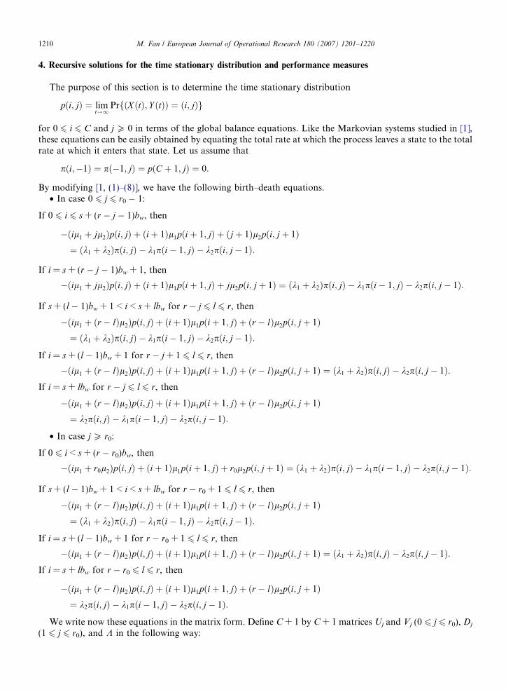
4. Recursive solutions for the time stationary distribution and performance measures

The purpose of this section is to determine the time stationary distribution

pði; jÞ ¼ limt!1

PrfðX ðtÞ; Y ðtÞÞ ¼ ði; jÞg

for 0 6 i 6 C and j P 0 in terms of the global balance equations. Like the Markovian systems studied in [1],these equations can be easily obtained by equating the total rate at which the process leaves a state to the totalrate at which it enters that state. Let us assume that

pði;�1Þ ¼ pð�1; jÞ ¼ pðC þ 1; jÞ ¼ 0:

By modifying [1, (1)–(8)], we have the following birth–death equations.• In case 0 6 j 6 r0 � 1:

If 0 6 i 6 s + (r � j � 1)bw, then

�ðil1 þ jl2Þpði; jÞ þ ðiþ 1Þl1pðiþ 1; jÞ þ ðjþ 1Þl2pði; jþ 1Þ¼ ðk1 þ k2Þpði; jÞ � k1pði� 1; jÞ � k2pði; j� 1Þ:

If i = s + (r � j � 1)bw + 1, then

�ðil1 þ jl2Þpði; jÞ þ ðiþ 1Þl1pðiþ 1; jÞ þ jl2pði; jþ 1Þ ¼ ðk1 þ k2Þpði; jÞ � k1pði� 1; jÞ � k2pði; j� 1Þ:

If s + (l � 1)bw + 1 < i < s + lbw for r � j 6 l 6 r, then

�ðil1 þ ðr � lÞl2Þpði; jÞ þ ðiþ 1Þl1pðiþ 1; jÞ þ ðr � lÞl2pði; jþ 1Þ¼ ðk1 þ k2Þpði; jÞ � k1pði� 1; jÞ � k2pði; j� 1Þ:

If i = s + (l � 1)bw + 1 for r � j + 1 6 l 6 r, then

�ðil1 þ ðr � lÞl2Þpði; jÞ þ ðiþ 1Þl1pðiþ 1; jÞ þ ðr � lÞl2pði; jþ 1Þ ¼ ðk1 þ k2Þpði; jÞ � k2pði; j� 1Þ:
If i = s + lbw for r � j 6 l 6 r, then
�ðil1 þ ðr � lÞl2Þpði; jÞ þ ðiþ 1Þl1pðiþ 1; jÞ þ ðr � lÞl2pði; jþ 1Þ¼ k2pði; jÞ � k1pði� 1; jÞ � k2pði; j� 1Þ:

• In case j P r0:

If 0 6 i < s + (r � r0)bw, then

�ðil1 þ r0l2Þpði; jÞ þ ðiþ 1Þl1pðiþ 1; jÞ þ r0l2pði; jþ 1Þ ¼ ðk1 þ k2Þpði; jÞ � k1pði� 1; jÞ � k2pði; j� 1Þ:

If s + (l � 1)bw + 1 < i < s + lbw for r � r0 + 1 6 l 6 r, then

�ðil1 þ ðr � lÞl2Þpði; jÞ þ ðiþ 1Þl1pðiþ 1; jÞ þ ðr � lÞl2pði; jþ 1Þ¼ ðk1 þ k2Þpði; jÞ � k1pði� 1; jÞ � k2pði; j� 1Þ:

If i = s + (l � 1)bw + 1 for r � r0 + 1 6 l 6 r, then

�ðil1 þ ðr � lÞl2Þpði; jÞ þ ðiþ 1Þl1pðiþ 1; jÞ þ ðr � lÞl2pði; jþ 1Þ ¼ ðk1 þ k2Þpði; jÞ � k2pði; j� 1Þ:
If i = s + lbw for r � r0 6 l 6 r, then
�ðil1 þ ðr � lÞl2Þpði; jÞ þ ðiþ 1Þl1pðiþ 1; jÞ þ ðr � lÞl2pði; jþ 1Þ¼ k2pði; jÞ � k1pði� 1; jÞ � k2pði; j� 1Þ:

We write now these equations in the matrix form. Define C + 1 by C + 1 matrices Uj and Vj (0 6 j 6 r0), Dj

(1 6 j 6 r0), and K in the following way:


U j ¼

uðjÞ0 0

l1 uðjÞ1

2l1. .

.

. .. . .

.

0 Cl1 uðjÞC

0BBBBBBBBB@

1CCCCCCCCCA; ð4:1Þ

where

uðjÞi ¼ �ðil1 þ jl2Þ for 0 6 i 6 C � jbw;

and

uðjÞi ¼ �ðil1 þ ðr � lÞl2Þ
for s + (l � 1)bw + 1 6 i 6 s + lbw with r � j + 1 6 l 6 r;
Dj ¼ l2 diagðjIC�jbwþ1; ðj� 1ÞIbw ; . . . ; Ibw ; 0IbwÞ; ð4:2Þ

V j ¼ diagðV ð0Þj ; V ð1Þ; . . . ; V ð1Þ|fflfflfflfflfflfflfflfflffl{zfflfflfflfflfflfflfflfflffl}j

Þ; ð4:3Þ

where

V ð0Þj ¼

k1 þ k2 �k1 0

k1 þ k2 �k1

. .. . .

.

k1 þ k2 �k1

0 k2

0BBBBBBB@

1CCCCCCCA;

which is an C � jbw + 1 by C � jbw + 1 matrix, and

V ð1Þ ¼

k1 þ k2 �k1 0

k1 þ k2 �k1

. .. . .

.

k1 þ k2 �k1

0 k2

0BBBBBBB@

1CCCCCCCA;

which is a bw by bw matrix; and

K ¼ �k2ICþ1: ð4:4Þ
In terms of matrices given in (4.1) to (4.4), we have
~pðjÞU j þ~pðjþ 1ÞDjþ1 ¼~pðjÞV j þ~pðj� 1ÞK for 0 6 j 6 r0 � 1; ð4:5Þ
and
~pðjÞU r0þ~pðjþ 1ÞDr0

¼~pðjÞV r0þ~pðj� 1ÞK for j P r0; ð4:6Þ

together with the normalization~p �~eT ¼ 1. If we denote D ¼ Dr0, U ¼ U r0

and V ¼ V r0, then by (4.5),~pðjÞ for

j P r0 can be determined by solving the following infinite system of linear equations

ð~pðr0Þ;~pðr0 þ 1Þ; . . .Þ ¼ ð~pðr0 � 1Þ;~pðr0Þ; . . .Þ

C0 0

C1 C0

C2 C1 C0

..

. . .. . .

. . ..

0BBBB@1CCCCA;


where C0 = �k2U�1 and, for k P 1,

Ck ¼ ðV þ k2U�1DÞU�1ð�DU�1Þk�1: ð4:7Þ

By (4.1) and (4.2), we obtain

�DU�1 ¼N 0

0 0

� �;

where N is a C � bw + 1 by C � bw + 1 lower triangular matrix with the following eigenvalues

ni ¼r0l2

il1 þ r0l2

for 0 6 i 6 C � r0bw

and

ni ¼ðr � lÞl2

il1 þ ðr � lÞl2

for s + (l � 1)bw + 1 6 i 6 s + lbw with r � r0 + 1 6 l 6 r. It is easy to see that

0 < nC�bw< � � � < n0 ¼ 1:

Thus, there exists a C + 1 by C + 1 invertible matrix T such that

DU�1 ¼ T diagðn0; . . . ; nC�bw; 0IbwÞT�1:

Consequently,

ðDU�1Þk ¼ T diagðnk0; . . . ; nk

C�bw; 0IbwÞT�1 for k P 1:

Moreover, kVk = 2k1 + k2 by (1.1) and (4.3). It turns out

kCkk 6 ð2k1 þ k2 þ k2kU�1DkÞkU�1kkICþ1 � DU�1kkTkkT �1k ð4:8Þ

for k P 1. We formulate now the recursive algorithm for ~pðjÞ as follows.

Theorem 4.1. Let R be the rate matrix given in (3.3). Then

~pðr0Þ ¼~pðr0 � 1ÞXkP0

RkCk;

which converges in the l1-norm. For j > r0,

~pðjÞ ¼~pðj� 1ÞR ¼~pðr0ÞRj�r0 :

For j = r0 � 1, . . . ,1,

~pðjÞ ¼ ð~pðjÞV j � k2~pðj� 1Þ �~pðjþ 1ÞDjþ1ÞU�1j :

For j = 0,

~pð0ÞU 0 ¼~pð1ÞV 0 �~pð1ÞD1 and ~p �~eT ¼ 1:

For the system with a finite waiting room of size K, one may follow the same algorithm to calculate~pðKÞ. Ob-serve that ~pðKÞðjÞ ¼~0 for j P [K/bw] + 1. Thus ~pðKÞðjÞ ¼~0 for j P [K/bw] + 2, and, for r0 6 j 6 [K/bw] + 1,

~pðKÞðjÞ ¼X½K=bw�

k¼j�1

~pðKÞðkÞCk�jþ1: ð4:9Þ


For the numerical example given in the end of Section 3, we have

U 0 ¼

0 0 0 0

1 �1 0 0

0 2 �2 0

0 0 3 �3

0BBBBB@

1CCCCCA; U ¼

�0:5 0 0 0

1 �1:5 0 0

0 2 �2 0

0 0 3 �3

0BBBBB@

1CCCCCA;

V 0 ¼

1:1 �0:7 0 0

0 1:1 �0:7 0

0 0 1:1 �0:7

0 0 0 0:4

0BBBBB@

1CCCCCA; V ¼

1:1 �0:7 0 0

0 0:4 0 0

0 0 1:1 �0:7

0 0 0 0:4

0BBBBB@

1CCCCCA;

D ¼ diagð0:5; 0:5; 0; 0Þ; K ¼ �0:4I4:

We conclude this section by the following performance measures: for~x ¼~p or~pðKÞ (resp.~x ¼~p or~pðKÞ), themean number of WB calls waiting for service found upon the arrival of any WB call (resp. at any time) is givenby

Q2f~xg ¼XC�r0bw

i¼0

XjPr0

ðj� r0Þxði; jÞ þXr

l¼1þr�r0;

Xsþlbw

i¼sþðl�1Þbwþ1;

XjPr�l

ðj� r þ lÞxði; jÞ;

the call (resp. time) probability of delay for WB calls is given by

P wf~xg ¼XC�r0bw

i¼0

XjPr0

xði; jÞ þXr

l¼1þr�r0;

Xsþlbw


XjPr�l

xði; jÞ;

and the call (resp. time) probability of blocking for NB calls is given by

P bf~xg ¼Xr

l¼r�r0;

XjPr�l

xðsþ lbw; jÞ:

Following Theorems 3.2 and 4.1, we have

Theorem 4.2. Let~v and ~di, 0 6 i 6 C, be vectors in RC+1 satisfying

~v ¼ ð0; . . . ; 0|fflfflfflffl{zfflfflfflffl}C�r0bwþ1

; 1; . . . ; 1|fflfflfflffl{zfflfflfflffl}bw

; . . . ; r0; . . . ; r0|fflfflfflfflffl{zfflfflfflfflffl}bw

Þ;

~di ¼ ð0; . . . ; 0|fflfflfflffl{zfflfflfflffl}i

; 1; 0; . . . ; 0|fflfflfflffl{zfflfflfflffl}C�i

Þ:

Then

Q2f~pg ¼~pðr0 � 1ÞR2ðI � RÞ�2~eTCþ1 þ~pðr0 � 1ÞRðI � RÞ�1~vT þ

Xr

l¼1þr�r0;

Xsþlbw


Xr0�1

j¼r�l

ðj� r þ lÞpði; jÞ;

P wf~pg ¼~pðr0 � 1ÞRðI � RÞ�1~eT

Cþ1 þXr

l¼1þr�r0;

Xsþlbw


Xr0�1

j¼r�l

pði; jÞ;

P bf~pg ¼Xr

l¼r�r0

~pðr0 � 1ÞRðI � RÞ�1~dsþlbw þXr0�1

j¼r�l

pðsþ lbw; jÞ !

;


and

Q2f~pg ¼~pðr0ÞR2ðI � RÞ�2~eTCþ1 þ~pðr0ÞRðI � RÞ�1~vT þ

Xr

l¼r�r0;

Xsþlbw


Xr0

j¼r�l

ðj� r þ lÞpði; jÞ;

P wf~pg ¼~pðr0ÞRðI � RÞ�1~eTCþ1 þ

Xr

l¼r�r0;

Xsþlbw


Xr0

j¼r�l

pði; jÞ;

P bf~pg ¼Xr

l¼r�r0

~pðr0ÞRðI � RÞ�1~dsþlbw þXr0

j¼r�l

pðsþ lbw; jÞ !

:

5. A comparison between systems with finite or infinite waiting rooms

In this section, we use the results for the systems with an infinite waiting room to investigate the systemswith a finite waiting room of size K, and to describe the convergence rate of the stationary distributions~pðKÞ and ~pðKÞ as K!1. We follow the approach of Simonot [6].

Assume that (m,k), (i, j) 2 X(K). Let

sðm;kÞði;jÞ ¼Xj

l¼0

pðm;kÞði;lÞ; sðKÞðm;kÞði;jÞ ¼Xj

l¼0

pðKÞðm;kÞði;lÞ;

and let ðUnÞnP1 be a sequence of i.i.d. random variables uniformly distributed on [0,1]. Then, by (2.13) and(2.14),

sðKÞðm;kÞði;jÞ ¼ sðm;kÞði;jÞ for k <K � m

bw

� �and j 6

K � mbw

� �;

sðKÞðm;kÞði;jÞ P sðm;kÞði;jÞ for k ¼ K � mbw

� �and r0 � 1 6 j 6

K � mbw

� �:

We construct now a couple of two-dimensional Markov chains ðX n; eY nÞ and ðX ðKÞn ; eY ðKÞn Þ by the followingalgorithm:

First, eY 1 ¼ eY ðKÞ1 ¼ 0.If ðX n; eY nÞ ¼ ðm; kÞ, then ðX nþ1; eY nþ1Þ ¼ ði; jÞ whenever

sðm;kÞði;j�1Þ < Un 6 sðm;kÞði;jÞ:

If ðX n; eY ðKÞn Þ ¼ ðm; kÞ, then ðX nþ1; eY ðKÞnþ1Þ ¼ ði; jÞ whenever

sðKÞðm;kÞði;j�1Þ < Un 6 sðKÞðm;kÞði;jÞ:

Observe that ðX n; eY nÞ and ðX ðKÞn ; eY ðKÞn Þ have the same transition probabilities as (Xn,Yn) and ðX ðKÞn ; Y ðKÞn Þrespectively.

Lemma 5.1. Assume that (m,k) 2 X(K) and K P C + r0bw.

(i) If ðX n; eY nÞ ¼ ðm; kÞ with k 6 r0 � 1, then ðX m; eY ðKÞm Þ ¼ ðX m; eY mÞ for n 6 m < L, where

L ¼ inf l l > n; eY l PK � m

bw

� �� :

(ii) Pr eY nþ1 6K�C

bw

h in o6 Pr eY n 6

K�Cbw

h in o:

Proof. Observe that, if k 6 r0 � 1, then k < K�mbw

h i. Part (i) can be obtained by the definition of the Markov

chains ðX n; eY nÞ and ðX ðKÞn ; eY ðKÞn Þ, (2.13) and induction. For part (ii), we write now

pnði; jÞ ¼ PrfðX n; eY nÞ ¼ ði; jÞg ¼ PrfðX n; Y nÞ ¼ ði; jÞg


and

~pn ¼ ðpnð0; 0Þ; . . . ; pnðC; 0Þ; . . . ; pnð0; jÞ; . . . ; pnðC; jÞ; . . .Þ:

Observe that ~pn ¼~p1Pn�1 and ~pnþ1 ¼~p2Pn�1, where P is the transition probability matrix given in (2.12).Moreover,

Pr eY nþ1 6K � C

bw

� �� ¼~pn �~eT

K�Cbw½ �þ1ð ÞðCþ1Þ;

It is clear that

~p2 �~eTK�Cbw½ �þ1ð ÞðCþ1Þ 6~p1 �~eT

K�Cbw½ �þ1ð ÞðCþ1Þ;

or equivalently,

ð~p1 �~p2Þ �~eTK�Cbw½ �þ1ð ÞðCþ1Þ P 0:

By using Theorem 2.1(iv) iteratively, we obtain that

ð~p1 �~p2ÞPn�1 �~eTK�Cbw½ �þ1ð ÞðCþ1Þ P 0:

This follows Pr eY nþ1 6K�C

bw

h in o6 Pr eY n 6

K�Cbw

h in o. h

Theorem 5.1. Let R be the rate matrix given in (3.3). Then

Pr ðX n; eY ðKÞn Þ 6¼ ðX n; eY nÞh i

¼ O RK�Cbw½ ��r0þ1

��
for all K P C + r0bw.
Proof. Let

Dðn;KÞ ¼ PrfðX n; eY ðKÞn Þ 6¼ ðX n; eY nÞg;
and let n and u be fixed positive integers. For r0 6 u 6 n and 0 6 m 6 C, we denote
un ¼ inffmjm P n� u; eY m 6 r0 � 1g;
and
snðmÞ ¼ inf mjm P un;X un ¼ m; eY m PK � m

bw

� �� :

Let now

D1ðn;KÞ ¼XC

m¼0

PrfeY ðKÞn 6¼ eY n; un 6 n; snðmÞ > ng;

D2ðn;KÞ ¼XC

m¼0

PrfeY ðKÞn 6¼ eY n; un 6 n; snðmÞ 6 ng;

D3ðn;KÞ ¼XC

m¼0

PrfeY ðKÞn 6¼ eY n; un > ng:

Observe first that D1(n,K) = 0 by Lemma 5.1(i). According to Lemma 5.1(ii), we have

Pr eY m PK � C

bw

� �� 6 Pr eY mþj P

K � Cbw

� �� ;


and hence

Pr eY m PK � C

bw

� �� 6

XjP K�C

bw½ �~pðjÞ �~eT

Cþ1

by letting j!1. This, together with Theorem 3.2, implies that

D2ðn;KÞ 6XC

m¼0

Pr supn�u<m6n

eY m PK � m

bw

� ��

6 ðC þ 1ÞXn

m¼n�uþ1

Pr eY m PK � C

bw

� �� 6 ðC þ 1Þu~pðr0 � 1ÞR K�C

bw½ ��r0þ1ðICþ1 � RÞ�1 �~eTCþ1

6 ðC þ 1Þ2uk~pðr0 � 1Þk1kðICþ1 � RÞ�1kkR K�Cbw½ ��r0þ1k:

Furthermore, if un > n, then eY n�u P r0; . . . ; eY n P r0. Together with the fact eY r0�1 6 r0 � 1, we obtain thatn � u P r0 and $m with r0 � 1 6 m 6 n � u � 1 satisfying eY m ¼ r0 � 1 but eY mþ1 P r0; . . . ; eY n P r0. This impliesthat

D3ðn;KÞ 6 Prfun > ng 6Xn�u�1

m¼r0�1

PrfeY m ¼ r0 � 1; eY mþ1 P r0; . . . ; eY n P r0g

¼Xn�u�1

m¼r0�1

PrfY m ¼ r0 � 1; Y mþ1 P r0; . . . ; Y n P r0g:

Let bm = the number of WB calls served during the time interval [tm, tm+1), and let am = 1 � bm. ThenYm+1 = Ym + 1 � bm = Ym + am, and hence

Y n ¼ Y m þ amþ1 þ � � � þ an�1: ð5:1Þ

If Ym P r0 � 1 and Ym+1 P r0, then

Prfbm ¼ kg ¼XC

m;i¼0

pðm;r0þk�1Þði;r0Þ

¼ ðC � r0bw þ 1ÞZ 1

0

ðr0l2tÞk

k!e�r0l2t dF2ðtÞ þ bw

Xr�1

l¼r�r0þ1

Z 1

0

ððr � lÞl2tÞk

k!e�ðr�lÞl2t dF2ðtÞ

by (2.3) and (2.7), and hence

Efbmg ¼XkP0

k � Prfbm ¼ kgP ðC � r0bw þ 1Þ r0l2

k2

P1

q> 1:

Moreover, am are i.i.d. distributed in case Ym P r0 � 1 and Ym+1 P r0. As in the proof of [6, Theorem 1],$ h P 0 such that d = E{exp(ham)} 2 (0,1). By combining this with (5.1), we obtain

PrfY m ¼ r0 � 1; Y mþ1 P r0; . . . ; Y n P r0g 6 PrfY m þ amþ1 þ � � � þ an�1 P r0g 6 Prfamþ1 þ � � � þ an�1 > 0g6 Prfexpðhðamþ1 þ � � � þ an�1ÞÞ > 1g 6 Efexpðhamþ1Þg � � �Efexpðhan�1Þg ¼ dn�m�1

for r0 � 1 6 m 6 n � u � 1. This implies that

D3ðn;KÞ 6Xn�u�1

m¼r0�1

dn�m�16

du

1� d:


Consequently,

Dðn;KÞ ¼ D1ðn;KÞ þ D2ðn;KÞ þ D3ðn;KÞ

6 infuPr0

ðC þ 1Þ2uk~pðr0 � 1Þk1kðICþ1 � RÞ�1k RK�Cbw½ ��r0þ1

�� þ du

1� d

� �:

Now we consider the case when r0 6 n < u, and set

s ¼ inffmjm > 1; eY m P K=bw½ �g:

Then

Dðn;KÞ ¼ Pr eY ðKÞn 6¼ eY n; s 6 nn o

þ PrfeY ðKÞn 6¼ eY n; s > ng:

Since

PrfeY ðKÞn 6¼ eY n; s > ng ¼ 0

by Lemma 5.1 (i) again, it gives that

Dðn;KÞ 6 Prfs 6 ng 6 Pr sup0<m6n

eY m P K=bw½ ��

6

Xn

m¼1

PrfeY m P K=bw½ �g

6 uk~pðr0 � 1Þk1kðICþ1 � RÞ�1kkR½K=bw��r0þ1k;

and hence

Dðn;KÞ 6 infðCþ1Þ2uPr0

fuk~pðr0 � 1Þk1kðICþ1 � RÞ�1kkR½K=bw ��r0þ1kg:

Therefore, Dðn;KÞ ¼ O RK�Cbw½ ��r0þ1

�� for all K P C + r0bw. h

Lemma 5.2. There exists a constant c > 0 such that
X½K=bw�þ1
j¼r0

k~pðKÞðjÞ �~pðjÞk1 6 cð½K=bw� þ 1Þk~pðKÞ �~pk1 þ ck~pðr0 � 1Þk1

XkP½K=bw�þ1

ðk þ 1ÞkRk�r0þ1k:

Proof. By Theorem 4.1 and (4.9),

~pðKÞðjÞ �~pðjÞ ¼X½K=bw �

k¼j�1

ð~pðKÞðkÞ �~pðkÞÞCk�jþ1 �X

kP½K=bw�þ1

~pðkÞCk�jþ1

for r0 6 j 6 [K/bw] + 1. Let c = supkP0kCkk, which is finite by (4.8). This, together with Theorem 3.2(ii),implies

X½K=bw�þ1

j¼r0

k~pðKÞðjÞ �~pðjÞk1 6 cX½K=bw�þ1

j¼r0

X½K=bw �

k¼j�1

k~pðKÞðkÞ �~pðkÞk1

!þ c

XjPr0

XkP½K=bw�þ1

k~pðkÞk1

!

¼ cX½K=bw �

k¼r0�1

ðk � r0 þ 2Þk~pðKÞðkÞ �~pðkÞk1 þ cX

kP½K=bw �þ1

ðk � r0 þ 2Þk~pðkÞk1

6 cð½K=bw� þ 1Þk~pðKÞ �~pk1 þ ck~pðr0 � 1Þk1

XkP½K=bw�þ1

ðk þ 1ÞkRk�r0þ1k;

which completes the proof. h

We formulate now the main result of this section as below.


Theorem 5.2. If 0 < h < 1/sp(R), then

limK!1

h½K=bw�k~pðKÞ �~pk1 ¼ limK!1

h½K=bw�k~pðKÞ �~pk1 ¼ 0: ð5:2Þ

Consequently,

limK!1

h½K=bw �jQ2f~pðKÞg � Q2f~pgj ¼ limK!1

h½K=bw�jQ2f~pðKÞg � Q2f~pgj ¼ 0;

limK!1

h½K=bw �jP wf~pðKÞg � P wf~pgj ¼ limK!1

h½K=bw �jP wf~pðKÞg � P wf~pgj ¼ 0;

limK!1

h½K=bw �jP bf~pðKÞg � P bf~pgj ¼ limK!1

h½K=bw �jP bf~pðKÞg � P bf~pgj ¼ 0:

Proof. First observe that sp(R) < 1 by Theorem 3.1 (i). We choose h 0 > 0 for which spðRÞ < 1=h0 < ð1=hÞ ^ 1and set e = h/h 0, then 0 < e < 1 and h = eh 0. By (1.2),

RK�Cbw½ ��r0þ1

�� 1= K�Cbw½ ��r0þ1ð Þ

< 1=h0

for K big enough. According to Theorem 5.1 and a slight modification on the proofs of [6, Corollaries 1 and 2],we have

k~pðKÞ �~pk1 ¼ OðkR K�Cbw½ ��r0þ1kÞ

for K P C + r0bw. Observe that

h½K=bw �kR K�Cbw½ ��r0þ1k < h½C=bw �ðh0Þr0�1e

K�Cbw½ � ! 0

as K!1. This implies that

limK!1

h½K=bw�k~pðKÞ �~pk1 ¼ 0:

Furthermore,

h½K=bw �ð½K=bw� þ 1Þk~pðKÞ �~pk1 ¼ e½K=bw �ð½K=bw� þ 1Þðh0Þ½K=bw�k~pðKÞ �~pk1 ! 0

as K!1, and

h½K=bw �X

kP K=bw½ �þ1

ðk þ 1ÞkRk�r0þ1k 6 ðh0Þr0�1e½K=bw �XkP1

k þ ½K=bw� þ 1

ðh0Þk¼ Oðe½K=bw�Þ

for K big enough. This implies that

h½K=bw �X

kP K=bw½ �þ1

ðk þ 1ÞkR½K=bw��r0þ1k ! 0

as K!1. By using Lemma 5.2, we have

limK!1

h½K=bw�XjPr0

k~pðKÞðjÞ �~pðjÞk1 ¼ 0:

Following the algorithm given in Theorem 4.1, we see that

limK!1

h½K=bw�k~pðKÞðjÞ �~pðjÞk1 ¼ 0

for j = r0 � 1, . . . , 0. Therefore,

limK!1

h½K=bw�k~pðKÞ �~pk1 ¼ 0:

We obtain the other limits by (5.2) and the definitions of the performance measures given in Theorem 4.2. h


Remark. By a minor revision on the proof of Theorem 5.2, we can obtain

Pr ðX n; eY ðKÞn Þ 6¼ ðX n; eY nÞn o

¼ Oðk~pðr0 � 1ÞR K�Cbw½ ��r0þ1k1Þ

for all K P C + r0bw. This implies that

limK!1

h½K=bw �k~pðKÞ �~pk1 ¼ 0 ð5:3Þ

even for 0 < h < 1=supkP1fk~pðr0 � 1ÞRkk1=k1 g. Observe that

supkP1

fk~pðr0 � 1ÞRkk1=k1 g 6 spðRÞ:

On the other hand, if h > 1=infkP1fk~pðr0 � 1ÞRkk1=k1 g, then

limK!1

h½K=bw �k~pðKÞ �~pk1 ¼ 1:

In fact, this limitation can be obtained by Theorem 3.2 and the following estimate

XjP½K=bw �þr0

k~pðjÞk1 PX

jP½K=bw�þr0

~pðjÞ��

��1

¼ k~pðr0 � 1ÞR½K=bw �þ1ðICþ1 � RÞ�1k1

P k~pðr0 � 1ÞR½K=bw �þ1k1=kICþ1 � Rk:

In particular, if g ¼ limK!1k~pðr0 � 1ÞRkk1=k1 exists, then the convergence rate in (5.3) is equal to 1/g. Unlike the

pure delay system discussed in [6], however, it is hard to calculate the exact convergence rate for a general loss-delay system.

6. Concluding remarks

By following the matrix-analytic approach, we have established a queueing model for the single link mixedloss-delay system with the exponentially distributed call holding time, the Markovian interarrival process forthe NB calls, and the general i.i.d. interarrival process for the WB calls. This is an efficient generalization of theprevious studied Markovian loss-delay systems [1].

The main issue of this paper is the theoretical analysis on the above mentioned queueing model. We havealso obtained the algorithmic solutions of the stationary probability distributions appearing in the systems.We refer to [5, Section 1.9] for the computational procedures. Once the rate matrix is known and the boundaryprobabilities for 0 6 j 6 r0 are calculated, the performance measures of the system is easily determined. Fur-thermore, the combined effect of blocking and delay can be measured by the following call and time powerfactors

PRf~pg ¼ 1� P bf~pg1þ l2Q2f~pg=k2

and PRf~pg ¼ 1� P bf~pg1þ l2Q2f~pg=k2

:

The effects of the bandwidth factor bw/C, the ratio l1/l2 and the cut-off parameter r0 on the system can also beexamined. Currently, a joint research project with Department of Computer Science at Dalarna Universityfocuses on a computational implementation of the described algorithms.

Acknowledgement

The author is grateful to Ernst Nordstrom for some stimulating discussions under the preparation of thispaper, and to the anonymous referee for his valuable comments.


References

[1] Y. De Serres, L.G. Mason, A multi-server queue, with narrow- and wide-band customers and WB restricted access, IEEE Transactionson Communication 36 (6) (1988).

[2] A. Feldmann, Characteristics of TCP connection arrivals, Technical Report, AT&T Labs-Research, 1998.[3] D.G. Kendall, Some problems in the theorem of queues, Journal of the Royal Statistical Society 13 (1951) 151–185.[4] L. Kleinrock, Queueing Systems, Vol. I: Theory, John Wiley & Sons, 1975.[5] M.F. Neuts, Matrix-Geometric Solutions in Stochastic Models, An Algorithmic Approach, Dover Publications, INC, 1981/1994.[6] F. Simonot, Convergence rate for the distributions of GI/M/1/n and M/GI/1/n as n tends to infinity, Journal of Applied Probability 34

(1997) 1049–1060.

a queueing model for mixed loss-delay systems with general interarrival processes for wide-band...

Documents