a race to compete for investment among indian states? – an
TRANSCRIPT
A Race to Compete for Investment among Indian States?
– An Empirical Investigation
Krishna Chaitanya Vadlamannati
Alfred-Weber-Institute for Economics University of Heidelberg, Germany
Abstract: India is a complex federal democracy where state level politics are dominated by state
specific issues rather than national issues, making the economic development of the respective
states the focal point of a potential electorate. As economic reforms are now driven by the states,
due to the withdrawal of controls exercised by central government in key areas, states are forced
to compete against each other in terms of attracting investment which would generate jobs and
boost their respective economies. Using spatial econometric estimations on panel data on 32
states in India during the 1991–2009 period (19 years), I indeed find that the inflow of
investment proposals in one state is positively correlated with investment proposal inflows
elsewhere (i.e., investment proposals related to Industrial Entrepreneurs Memorandums coming
from other states for approvals, increase the likelihood of Industrial Entrepreneurs Memorandum
proposals coming from the state in question). While high income states compete for investment
both among themselves (intra-group) and with low income states (inter-group), the competition
is largely confined to within-group in the case of low income states. The results are robust to
alternative weighting schemes, samples, methods, and controlling for the possibility of
endogeneity.
Keywords: Investments, Spatial econometrics, India (F21; R58; O53).
------------------------------------------------- Author’s note: I thank Axel Dreher for the discussion on spatial econometrics and Ron Davies for providing a detailed list of comments on the previous draft. The data and do files for replicating the results can be obtained upon request. A slightly different version of the paper was presented at the South Asia Institute, Heidelberg. I thank Subrata Mitra and participants for their comments.

“India Looks to the States: While New Delhi idles, India's large and diverse states are competing
for growth and investment.”
– The Wall Street Journal, April 20111 “When did we say that we would not touch American capital? Investments generate employment
and so by wooing American investment the chief minister is not going beyond the party’s line.”
– Communist Party of India (Marxist)’s senior leader Shyamal Chakraborty defending West Bengal’s CPI(M) Chief Minister Buddhadeb Bhattacharya in 20072.
1. Introduction
Do states in India compete for investment? As the opening quotes illustrate, in India today the
state governments are desperate to attract private and foreign investment by removing policy
bottlenecks that are often viewed as unattractive to firms (Aghion, Burgess, Redding and
Zilibotti 2008). Many in the industry feel that this sort of competition is good for the respective
states as it not only helps solve problems associated with excessive bureaucratic controls,
corruption and creating an investment friendly atmosphere, but also creates enormous job
opportunities which form huge political capital for incumbent politicians. Therefore, there is
every reason to believe that states in post-reform India tend to compete for investment (The Wall
Street Journal 2011, Kanta 2011). For instance, Kanta (2011), Schneider (2004) and Venkatesan
(2000) cite examples of large tax and other fiscal incentives the states within India offer to attract
investment. In this paper, I examine whether states in India compete for big ticket investment
proposals. While there is a growing literature estimating the extent of the competition in
international taxation and environmental policies, policy reforms and labour standards, to the
best of my knowledge there is no empirical evidence examining the potential competition among
states within India, a gap the current paper fills.
1 See: http://online.wsj.com/article/SB10001424052748704099704576288611078352574.html?mod=WSJ_topics_obama 2 See: http://www.indiastrategic.in/topstories57.htm

Spatial econometrics has been used in the literature to examine the race to the bottom
arguments regarding taxes, environmental regulations, economic policy reforms and labour
standards. The first group of work includes Davies, Egger and Egger (2003), Devereux,
Lockwood, and Redoano (2008), Davies and Voget (2008), Overesche and Rinke (2008) and
Klemm and van Parys (2009), who focused largely on tax competition to attract FDI between
developed countries. Here, they find a positive spatial lag, meaning that as tax rates fall in one
nation, this lowers tax rates elsewhere. Likewise, in the environmental literature, Markusen,
Morey and Olewiler (1995), Fredriksson and Millimet (2002), Beron et al. (2003), Murdoch et
al. (2003), Levinson (2003) and Fredriksson et al. (2004), Davies and Naughton (2006) and
Perkins and Neumayer (2010) focused on the joint adoption of environmental agreements and
interaction in environmental policies. These studies tend to find evidence consistent with the race
to the bottom argument. Focusing specifically on spatially weighted third-country determinants
of inbound and outbound FDI, Blongien et al. (2007) and Baltagi et al. (2007) provided empirical
support for the existence of various modes of complex FDI. Extending the analysis to labour
standards, Davies and Vadlamannati (2011) find strong evidence of the potential race to the
bottom in labour standards, i.e., labour rights in one country depend on those elsewhere. On the
contrary, Neumayer and de Soysa (2011) find support for a race to the top with respect to
women’s labor rights in foreign countries with which a country is connected via trade and FDI.
Interestingly, Cho, Dreher and Neumayer (2011) also find evidence of a race to the top with
respect to human trafficking policies across countries. Using the Economic Freedom Index as a
measure of policy liberalization, Pitlik (2007) and Gassebner, Gaston and Lamla (2011) find
strong evidence of a race to the bottom among European and developing countries to liberalize
regulatory, monetary and trade policies. Similar such findings were echoed by Simmons and

Elkins (2004). Finally, Elkins, Guzman and Simmons (2006) also find evidence of a race to the
bottom with respect to bilateral investment treaties.
While there is a growing literature estimating the extent of the competition in areas
related to taxation, environment, labor standards, investment treaties and economic policy
reforms internationally, evidence on the potential impact of competition to attract investments
(domestic and foreign) within a country is scarce. Coughlin and Segev (2000) is an exception,
testing for the existence of spatial heterogeneity and spatial dependence in FDI inflows within
China. This is the gap the current paper fills by specifically focusing on competition among
Indian states in new investment policy during the post economic reforms period. While several
papers on India have considered the impact of factors at the local level in attracting FDI
(Nunnenkamp and Mukim 2011a, b), empirical studies estimating whether there is indeed
strategic interaction in investment policies, i.e., whether there is evidence of interstate
competition within India for big ticket investments, is absent. Beginning with a simple
conceptual note explaining why states in India compete for large investment proposals, the paper
models spatial autoregressive relationships among states to attract investment proposals.
Using information on large investment proposal approvals in 32 Indian states during the
1991–2009 period, I find that the inflow of investment proposals in one state are positively
correlated with the investment proposal inflows in other states. Furthermore, I find that industrial
or high income states compete for investment among themselves, as well as with low income
states. On the other hand, low income states seem to compete only among themselves. I interpret
these results as direct evidence of interstate strategic interactions in investment policy. I find that
investment policies are strategic complements, a key requirement for finding a ‘race to the
bottom/top’ in attracting investments. Since there is a noticeable upward trend in investment

proposals being put up for approval over the sample period, one might consider this evidence as
a race to the top. However, critics of globalization might well consider this as an evidence of
race to the bottom, citing large anecdotal evidence reported in press, media and NGO reports on
the side-effects (such as lapses in environmental regulations, labor standards, land acquisition
policy and revenue foregone from tax incentives) emanating from such fierce competition to
attract investment. Overall, if the benefits associated with such competition outweigh the costs,
then such competition is welcome. On the other hand, if there are less overall benefits than costs,
then such fierce competition might well be the path towards mal-development. I leave it to
future research, perhaps by usefully employing the comparative case study method, to examine
whether fierce competition among states is necessarily leading to race to the bottom, or
otherwise.
The rest of the paper structured as follows. Section 2 illustrates why states in India
compete for investments. Section 3 describes the methodology adopted and the data. Section 4
discusses the results and Section 5 concludes.
2. Competition between Indian States
In an extremely diverse country like India, when a private or foreign firm intends to
undertake large scale investment, usually they narrow their options down, after extensive
research, to a few specific potential destinations (states) for various reasons. Often, this results in
intense competition among those potential states to attract big ticket investment. One such
example is Tata’s new Nano car project in 2008, which after withdrawing from the West Bengal
state, was offered several packages by other states including Karnataka (in the outskirts of
Bangalore), Maharashtra (in Pune), Andhra Pradesh (near Vizag) and Gujarat. After studying
each possible location, the decision to locate the project in Gujarat was finally taken by the firm.
It was widely cited in the Indian media that the Gujarat state offered free land, commitment to
construct new roads near the project site, and initiate employee training programs hosted at the
site (Businessweek 2008, Business Standard 2008). Over the years, such incentives offered by
states in India to attract large scale investment projects have not only increased drastically, but
have become commonplace. In fact, Kanta (2011), Schneider (2004) and Venkatesan (2000) cite
numerous examples of large tax and other fiscal incentives offered by states within India to
attract investment.
It began in 1991, when the government of India embarked upon a series of economic
liberalization measures, thus ending the ‘license and permit raj’ which required firms to obtain
licenses from the central government of India, not only for setting up businesses, but even for
expansion and increasing their production capacity. The objective behind such restrictive policy
was to spread investment evenly across the states. Instead of creating a balanced regional
development, however, the ‘license-raj’ did not allow firms to benefit from economies of scale.
In addition, Biswas and Marjit (2002) find that industrial licences were granted to the states
based on the political considerations of the central government. Thus, this licensing system was
also subject to political manipulation leading to market distortions created by political incentives.
The system was abolished in 1991 and since then, industrial firms with investments of Rs. 10
crores (20 US$ million) in the manufacturing sector, and Rs. 5 crores (10 US$ million) in the
services sector, are now only required to file information in the Industrial Entrepreneurs
Memorandum (IEMs hereafter) with the Secretariat of Industrial Assistance in New Delhi.
Thereafter, no further approvals are required. The IEMs basically originate from each state every
(month) year after finalizing business proposals, and acquiring all the required permission from

the respective state governments where investments are proposed. Thus, IEMs coming from state
i in year t reflects the openness of the prevailing investment environment in that particular state.
Since economic liberalization, two things have changed dramatically. First, increasing
reliance on markets, which has proven to be an enabling factor for the emergence of a market
economy driven by the states and not by the center. This is result of a major shift in the role of
the center and the states in the economic policy decision making process. Post 1991, the
dominance of the center in economic policy decision making has significantly diminished,
paving way for the state governments to design their own policies. This has effectively meant
that economic reforms are now driven by the states, due to the withdrawal of controls exercised
by the central government in key areas, including things like issuing industrial licenses and other
types of control over private investment (Ahluwalia 2000)3. Rudolph and Rudolpah (2001)
highlight the role of state governments in the Indian economy. According to them, in recent
years, aggressive competition among states for private and foreign investment has attracted the
attention of the media and policy makers locally and internationally. In addition, there was a
marked decline in public investment, which coincided with a rapid increase in private
investment. As a consequence, the center’s financial leverage over the states declined steadily as
states looked more and more towards attracting private and foreign investment to finance their
investment requirements. Khemani (2007) and Arulampalam et al. (2009) show how the central
government allocated financial transfers to the state governments purely based on political
considerations, leading to equity and efficiency distortions4. As a result of opening their doors to
investment, economic factors predominantly determined the number and magnitude of
3 For instance, state governments started to play an active role in areas related to industrial promotion, releasing state-specific industrial policies which were previously absent, land acquisition for industrial purposes, provision of infrastructure, tax concession (excluding corporate taxes), approval of Special Economic Zones, among others. 4 Also, see Singh and Garima (2004) for similar such arguments and analysis.
investment inflows into the states5. In the process, states which possessed location advantages
such as larger markets, better infrastructure, a more skilled labor force, and the presence of a
large investor base in comparison to less well-endowed states, started to benefit (Kanta 2011,
Kohli 2004, 2006, Basley et al. 2007, Ahluwalia 2000). This in turn put more pressure on less
developed states, and all states for that matter, to increase their competitiveness in order to gain
investment. In addition, if the benefits associated with these investments do in fact spillover in to
other states in the country, then this agglomeration (in the case of private and foreign
investments) might lead to more investment proposals coming from the other states.
Second, in a complex federal democracy such as India, after the 1991 economic reforms,
state level politics have been dominated by state specific issues rather than national issues,
making the economic development of the respective states the focal point of a potential
electorate (Ahluwalia 2000). In fact, the rewards of competing for investment can be derived
from the basic international trade models such as ‘Heckscher-Ohlin theory’, Ricardo-Viner type
models, and the ‘ideology and inequality thesis’ of Dutta and Mitra (2006), which predict that
trade would extensively benefit those countries with abundant factors of production compared to
countries with scarcer factors. Since developing countries like India are labor rich and capital
poor, their openness to trade is expected to benefit the poor labor force, while hurting domestic
rent seeking forces (Bhagwati 2004). The same logic also applies for private and foreign
investment, and the barriers associated with them. As an economy opens up to private and
foreign investment, current exploitative rent seeking forces start competing with new investors
for market and labor (Jakobsen and de Soysa 2006, Srinivasan 1987). Since new investment,
particularly high end investment and FDI, creates quality jobs that are associated with higher
5 See Subramanian (2008) for an excellent analysis on India’s recent growth and its integration into the world economy.

wages and better working conditions than existing local firms, as well as most likely altering
labor market conditions in the long run (Brown, Deardorff and Stern 2004), there are significant
benefits for the labor force associated with the process of attracting investment into the state. As
large sections of the middle class stand to gain, the median voter too will prefer those
governments or incumbents which support capital importation (Bhagwati 1999). Note that the
post 1991 period also coincides with a dramatic surge in political participation of lower caste
communities who remain economically backward with the highest rate of unemployment, putting
pressure on state governments to provide employment opportunities6. Thus, state governments
are forced to compete against each other in attracting investment which would not only generate
jobs and boost their economies, but also increase their chances of reelection.
3. Empirical Methodology and Data
In this section, I describe both the data I use, which is a panel data set across 32 Indian
states during the 1991–2009 period, and the estimation specification.
3.1 Estimation Specification
The baseline specification estimates the IEM proposals coming from state i in year t
which were approved, as a function of a set of exogenous variables itZ :
)1(tiitiit ZIEM
Where, i is the state-specific dummy and ti
is the error term. The control variables are drawn
from the existing literature on determinants of investment in general and FDI, and are described
below. In line with the traditional FDI literature, to this baseline, I introduce the IEM proposals
6 Scheduled Castes (SCs), Scheduled Tries (STs) and Other Backward Castes (OBCs) form the lower castes in India. According to Prakash and Chin (2009), 46% of the ST and 37% of the SC population is living below the official poverty line defined by the Indian government.

coming from other states for approvals in year t, a variable known in the literature as the spatial
lag. Specifically, I estimate:
)2(tiiititjit
ijiit ZIEMIEM
Where, itjitij
IEM
is the spatial lag, i.e., the weighted average of IEM proposals of other
states put up for approval. For weights, following Davies and Vadlamannati (2011), I utilize
ikkt
jt
ijtGDP
GDP . In words, the share that state i gives to state j is equivalent to j’s share of the
total GDP across all states in India, not including state i.7 It is, however, noteworthy that the sum
of the weights across other states for state i observation will equal 1. This weighting scheme
imposes the assumption that bigger states get higher weights. The rationale for using state GDP
as the weight is two-fold. First, one might anticipate that state i pays more attention to what is
taking place in larger states rather than small ones. Second, when the goal of manipulating
investment policy is to attract investment, this will depend on the elasticity of investment to a
given state’s policies. Thus, if state j (Maharashtra, which attracts a large number of IEMs, see
figure 1, and has a GDP share in India’s total GDP of about 17%) is already attractive for
investors relative to state k, then a change in j’s (Maharashtra’s) investment policy has a larger
impact on the allocation of investment than a comparable change in k. This, in turn, would make
i more responsive to j’s (Maharashtra’s) investment policies than to k’s, a difference that is
reflected in equation (2) by giving a greater weight to j. In addition to this, traditional FDI
literature also shows that FDI is attracted to larger countries (see Blonigen 2005), this would
7 As described by Anselin (1988) and Plümper and Neumayer (2010), it is common to row standardize the weights so that the sum of the weights adds up to one.

imply a greater sensitivity on the part of state i to the investment policies of a large state in India.
This apart, several papers in the race to the bottom or cross-country competition literature have
used GDP as a weight (Devereux, Lockwood, and Redoano, 2008, Madariaga and Poncet 2007,
Pitlik 2007). As mentioned before, I include state fixed effects to control for unobserved state
specific heterogeneity in the panel dataset, and ωit is the error term. It is noteworthy that I do not
estimate the model using time dummies because of the way the spatial lag is constructed, which
is strongly correlated across states in a given year. For example, when moving from the lag for
Assam to that of Punjab, I am essentially taking Punjab’s GDP weighted IEMs out of the spatial
lag and replacing them with Assam’s. Instead, I include a time trend to capture other factors
which are not accounted for in the model such as efficiency gains through technological
advancements or enhanced management skills. These usually grow over time and can be
expected to have a positive correlation with attracting investment. This apart, the time trend
applied here from 1991 also captures the trend in economic reforms which were launched in
1991. Finally, this baseline specification is then modified to explore the robustness of the main
findings. The specifics of these modifications are described in the results section.
As the dependent variable here is a count of IEM proposals, the preferred estimates are
those from the maximum likelihood negative binomial regressions reported as under:
)3()(exp]|[ itjitit ZZIEME
Where, Zit is the vector of other explanatory variables to be employed in the model
including the spatial lag, and is a parameter that captures whether the data exhibits over
dispersion. The variance of counts in the negative binomial model is:
)4()(exp)]/1(1[]|[ 2 ititit ZZIEMVar
So, the variance to mean ratio (i.e., the dispersion) in this model is given by: ( +1).
Where if > 0, the variance grows faster than the mean and the data exhibits over dispersion,
and where = 0, the negative binomial model paves way for a Poisson model, which, by its
very construction, restricts the variance equal to the mean. Since the resulting count variables
here, namely the number of IEM proposals approved, show a distribution which is strongly
skewed to the right (with an accumulation of observations at zero) and also display significant
over dispersion (with the variance being greater than the mean, see descriptive statistics in
appendix 3), I employ the negative binomial estimator over the poisson method (Lawless 1987,
Cameron and Trivedi 1998) with heteroskedasticity consistent robust standard errors (Beck and
Katz 1995). Furthermore, the results of the ‘goodness-of-fit’ test support using negative binomial
over the poisson estimation method.
3.2 Data
I use annual data for 32 Indian states from 1991 to 2009. The list of states is in the appendix. For
the dependent variable, I use the total number of investment proposals, namely the Industrial
Entrepreneur Memorandums (IEMs) coming from each state i in India in financial year t
approved by the Secretariat of Industrial Assistance (SIA hereafter) of the Department of
Industrial Policy and Promotion (DIPP). These data are published every year in aggregate form
by each state in DIPP’s various annual report issues. Post 1991, with the inception of the New
Industrial Policy Resolution 1991, all industrial undertakings (private or foreign) are exempt
from obtaining an ‘industrial license’ to manufacture goods and services anywhere in India.
However, a few industrial sectors are reserved for obtaining industrial licenses, namely (a)
industries reserved for the Public sector, (b) industries retained under compulsory licensing, (c)
items of manufacture reserved for the small scale sector, and (d) if the proposal attracts

locational restriction. Barring these few restricted sectors, industrial undertakings (private or
foreign) are exempt from obtaining an ‘industrial license.’ Instead, firms are required to file an
Industrial Entrepreneur Memoranda (known as IEM) (Part ‘A’) in the prescribed format of the
Industrial Policy Resolution with the SIA. Upon filling Part A of the form, the undertaking
would receive an acknowledgement receipt containing an SIA registration number. Beyond this
form, there is no further approval which is required to start a business in a state. It is also
noteworthy that prior to 1991, public, private or foreign firms would have required additional
industrial licenses even to expand their business operations or increase their production. Under
the new guidelines, expansion of business can be done by filling an IEM with the SIA.
Immediately after commencement of commercial production, Part B of the IEM has to be filled
out in the prescribed format. Thus, to start a business, investors must file IEMs giving details of
the proposed project. The data on IEM proposals does not contain details of actual
implementation.
A few important points are worth noting here. Biswas and Marjit (2002) show that the
industrial licenses approved by the central government of India prior to 1991 (to set up
businesses in respective states) were driven by political rather than economic considerations.
Obviously, one might also presume that IEMs which are filed at the SIA in New Delhi are also
subject to such political manipulation. There are several reasons why I believe that such concerns
are not applicable to IEMs. First, IEMs are not like erstwhile licenses for which undertakings had
to seek permission from the central government of India in the ‘license raj’ period. Rather, IEMs
are simply a form providing information to the respective authorities (i.e., SIA) about the
establishment and other details of the firm. Moreover, the SIA in New Delhi, a non-political
institution, collects the information on IEMs approved for statistical purposes which are in no
way associated with political manipulation or state lobbying. Second, although IEMs are given
token approvals by the SIA, many of the establishment deals related to land acquisitions, tax
concessions, environment, pollution, electricity, water and other clearances, and other
bureaucratic permissions related to stating businesses, are done through discussions and
consultations with the respective state government agencies and departments. Therefore, in order
to attract more investment into the state, the respective state governments are willing to provide
numerous concessions to large industrial firms, reduce bureaucratic hurdles, and speed up the
process of gaining permission and clearances required to set up a business. Naturally, the firm
would also want to locate itself in the state which provides the maximum number of concessions
to attract new investment (e.g., see Kanta 2011). Therefore, it is reasonable to expect that a firm
would apply for an IEM only after obtaining the required clearances from the respective state
governments. The SIA would however use its discretion in cancelling the IEM proposal only if is
found that the specific proposal contained in the IEM is able to be licensed. Third, it would also
be safe to presume that the number of IEMs originating from a particular state in year t mirrors
the prevailing investment friendly environment created by that state government. Therefore,
approval of IEMs originating from state i in year t must be seen more as a part of a ‘push efforts’
strategy adopted by respective state governments competing for investment, rather than an
instrument which can be used to serve political interests.
The vector of control variables includes other potential determinants attracting IEM
proposals into state i during year t, which I obtain from the extant literature on the subject. Since
this is the first such study on IEMs in India, I follow other pioneer studies on determinants of
FDI and FDI policy reforms: Blonigen et al. (2007), Blonigen (2003), Blonigen and Figlio
(1998), Wheeler and Moody (1992), Coughlin et al. (1991) and other comprehensive evaluations

of these early studies on FDI (Kobrin 2005, Chakrabarti 2001). Dunning (1993) proposed that
the location factor is the key to attracting foreign investment into a country. I believe this would
also be similar in the case of private investment. Some of these location specific factors include:
market growth, economic development, institutions, infrastructure, availability of natural
resources, and government policies. Accordingly, the models control for the effects of market
size by including respective state GDP (logged) in Indian rupees (1993-94 constant prices) and
the states’ economic growth rates obtained from the Reserve Bank of India’s dataset. Following
Dreher et al. (2010), I also consider the total population (log) as data on the total labor force is
not available on a yearly basis for states in India.
Good infrastructure facilities increase the productivity of investment, which in turn helps
in attracting more investment (Wheeler and Mody 1992, Asiedu and Lien 2004). Since there are
various factors which contribute to the development of infrastructure like roads, ports,
telecommunications, power, railways and so on, it becomes quite difficult to capture data for all
of these variables for any given state due to a lack of data availability. I thus include the
electricity consumption of state i in year t in kilowatts. The main reason for considering this
variable is that it not only captures the availability of electricity, but also its cost. Likewise, I also
include a proxy for industrialization by including the industry share in a state’s GDP, seeing as
most of the IEM proposals are big ticket industrial investment projects and are attracted to
industrial states. The other contentious issue in India is the effect of labour market rigidities.
Many argue that the effect of labor market rigidities is more pronounced and discourages FDI as
well as domestic investment (Ashan and Pages 2009, Aggarwal 2007, Basely and Burgess 2002).
Chief economic advisor to the Prime Minister of India, Kaushik Basu (2005), argues that apart
from promoting other factors, India will needs to attempt to carry out drastic labor market
reforms. However, due to stiff political opposition, any major change in labor laws is often ruled
out8. Following Teitelbaum (2011), Aghion et al. (2008), and Basely and Burgess (2002), I
include man days lost in state i in year t due to strikes and lockouts as a proxy for labor market
rigidities in India. Using the information from the SIA on new industrial policy adopted by the
respective states, I code the value 1 for the year in which new industrial policy was adopted by
states, and 0 otherwise. Finally, following Basely and Burgess (2000), I also capture the number
of years in which either the Indian National Congress (INC hereafter) - centre-left in ideology,
Bharatiya Janata Party (BJP henceforth) - centre-right, Left Front led by the Communist Party of
India-Marxist (CPI-M) – leftists, and regional parties, often considered as soft left, were in
power in state i in year t, in order to control for the ‘ideology hypothesis’ (Dutt and Mitra 2006).
Accordingly, I expect that the number of years parties with a center-left ideology were in power
will have a positive impact on IEM proposals coming from that state. Lastly, I include a dummy
for President’s rule imposed in the state by the central government to account for political
uncertainty9.
3.3 Endogeneity concerns
The difficulty with the spatial lag is that if investment policy in state i depends on that in
state j, and vice versa, the spatial lag is endogenous. In order to address these endogeneity
concerns, I utilize non-linear instrumental variable estimations. Following standard spatial
econometric procedure, for the instruments I use jtjitij
Z
, that is, the weighted average of
the other states’ economic variables, namely the state GDP growth rate, the share of industry in
8 For a detailed argument on labor market rigidities and required reforms, see Basu’s (2005) article from the BBC: http://news.bbc.co.uk/2/hi/south_asia/4103554.stm. 9 President’s rule is often imposed by the central government based on the recommendations provided by the respective state’s governor. Imposing President’s rule requires dismissing the state legislative assembly, with powers vested to the state governor until fresh state legislative assembly elections are called.

total state GDP, a state’s industrial policy, man days lost in strikes and lockouts, population, and
infrastructure. The intuition behind using these variables is twofold. First, economic variables
such as market size, industrialization, labor force and industrial policy are found to be very
important in attracting investment into states. Second, for a given state j, its economic exogenous
variables directly impact its investment policies but are not dependent on those in state i.
Therefore they are correlated with the endogenous variable, but are themselves exogenous,
making them suitable instruments.
The normal procedure in the next step would therefore be to utilize an instrumental
variable method using two-stage least squares (2SLS – IV hereafter). However, employing
instrumental variables in non-linear models such as negative binomial may not only be
problematic, but also difficult to perform. Therefore, I manually run the instrumental variable
regressions for negative binomial models by regressing endogenous variables – spatial lag (of
IEMs) – on the selected instrumental variables by using the negative binomial models (which are
the first stage regressions). I then predict the values of the endogenous variable and regress the
dependent variable – IEM proposals approved – using negative binomial estimations,
respectively (the second stage regressions). The 2SLS–IV estimations with state fixed effects are
employed to check the validity of the instruments which are discussed below.
The validity of the selected instruments depends on two conditions. First, instrument
relevance, i.e., they must be correlated with the explanatory variable in question – otherwise they
have no power. Connected to this, Bound, Jaeger and Baker (1995) suggest examining the F-
statistic on the excluded instruments in the first-stage regression. The selected instrument would
be relevant when the first stage regression model’s F-statistics meets the thumb rule threshold of
being above 10 (Staiger and Stock 1997). Second, the selected instrument variable should not

vary systematically with the disturbance term in the second stage equation, i.e., 0itit IV . In
other words, the instruments cannot have independent effects on the dependent variable. As for
the exclusion restriction, I know of no theoretical or empirical argument linking the exogenous
variables of state j to a direct impact on the IEM proposals coming from state i for approval.
Nevertheless, a Hansen J-test is employed to check whether the selected instruments satisfy the
exclusion restriction (results provided at the end of the regression tables).
4. Empirical Results
4.1 Baseline Results
Table 1 presents the baseline results and the summary of data statistics are presented in appendix
4. While table 2 focuses exclusively on high income states, tables 3 examines the results related
to low income states (also known as special category states), estimated using negative binomial
regression estimations. Note that the results in all tables report marginal effects at the mean of
explanatory variables10. Beginning with column 1 of table 1, I show results without including the
spatial lag to ease the comparison between my results and any other study on determinants of
IEMs. As expected, I find that industrial states, better infrastructural facilities, and having an
industrial policy framework in place, tend to attract more IEM proposals. After controlling for
state-specific fixed effects, however, other controls remain insignificant. In column 2, which
forms my preferred specification, I include the IEM spatial lag term. As can be seen, I find a
positive and significant spatial lag which is significantly different from zero, at the 1% level. To
interpret the marginal effect, a standard deviation increase in the IEM approvals of all other
states would increase the IEM approvals in state i by roughly three proposals. As seen from the
last column of table 1, the positive significant effects of the spatial lag term remain robust in the
10 I use the Stata 11.0 margins command to calculate marginal effects.

IV models (see column 3). The substantive effects here suggest that a standard deviation increase
in the spatial lag of the IV models is associated with an increase in IEM approvals in state i by
roughly three proposals. Since the spatial lag term is positive, this can be interpreted as evidence
of strategic complementarity. While strategic complements can theoretically result in a
meaningful race to the bottom or top, we leave it up to future research, perhaps usefully
employing the comparative case study method, to examine whether fierce competition among
states necessarily leads to race to the bottom or otherwise.
Before moving further, it is necessary to discuss the validity of the selected instruments,
which depends on the two aforementioned conditions, namely instrument relevance and
exclusion criteria. The instruments have passed in both cases as reported in table 1, which speaks
to the strength of the instrument. As highlighted earlier, I estimate 2SLS-IV models that report
the statistics which explore the strength of the instruments. As seen, the first-stage F-test and
Anderson canon LR statistics report the test statistic used to test the null hypothesis; i.e., the
parameter estimate for the instrument in the first stage regression is equal to zero. Based on
Staiger and Stock (1997), I treat F-statistics greater than 10 as being sufficiently strong. In table
1, I find that in column 3, the F-statistic is greater than 10 and significantly different from zero,
at the 1% level. Finally, the Hansen J-Statistic also shows that the null hypothesis of exogeneity
cannot be rejected at the conventional level of significance.
4.2 Results for different regional categories
In Table 2, I divide the states into two different groups based on the classification of the Indian
government, namely non-special category states and special category states. The non-special
category states are basically high income states and are more advanced in terms of
industrialization. While the special category states are low income states which are not only less
industrial, but also suffer from higher levels of poverty and chronic underdevelopment. There are
a total of 14 special category and 18 non-special category states in the sample I use here. The
first four columns of table 2 capture the results for non-special category states (high income
states hereafter), and the last four columns report the results related to special category states
(low income states henceforth). I divide the states into two because of the concern that the results
may be driven by the high income states, i.e., relatively advanced states with high levels of
industrialization and infrastructure readily available to attract investment, a point noted by Kanta
(2011), Kohli (2006) and Ahluwalia (2000). Note that here (as well as in all subsamples below),
I recomputed the spatial lag and the instruments using only those states in the subsample, i.e.,
assigning those outside of the subsample zero weight. This implicitly assumes that there is only
competition within a subsample. To be more specific, when I estimate the models related to high
income states, I create the spatial lag and instruments using only high income states. The same
goes for estimating the low income states sample.
At first glance, it can be seen in table 2 that the results for the high income and low
income subsamples are comparable to those for the main sample reported in table 1, indicating
that the results are not being driven by either of the two samples. In column 1, I find a strong
positive impact of the spatial lag term on IEM approvals in high income states, which is
significantly different from zero, at the 1% level. The substantive effects show that a standard
deviation increase in the spatial lag term is associated with roughly 34 more IEM approvals after
holding other variables at their mean. After controlling for endogeneity in column 2, I find that
the positive significant effects remain. The substantive effects, however, increase when the
potential reverse feedback effects are controlled for. A standard deviation increase in the spatial

lag term of the IV estimations is associated with an increase of 84 IEM approvals in high income
states after holding other covariates at their mean.
In column 3, I expand the analysis by also considering cross-group competition. In these
regressions, the spatial lag for high income states is calculated using only the high income states,
with the spatial lag of the low income state variables calculated in a comparable way. Note that
in constructing these instruments, this means that I now have two versions of each weighted sum
of an exogenous variable, with one corresponding to each group. As seen, I find higher levels of
competition for IEM proposals, both within-group and cross-group, for high income states. Both
the high income and low income IEM spatial lags are significantly different from zero, at the 1%
level (see column 3). Likewise, after controlling for endogeneity, I find that these results remain
robust and significant, at the 1% level. Note that the instruments used here pass both the test of
instrument relevance and exclusion criteria. The next four columns in table 2 capture low income
states. In column 5, I find that the spatial lag term is positive and significantly different from
zero, at the 1% level. Controlling for endogeneity, the results also remain robust. After
controlling for reverse feedback effects using IV estimations, a standard deviation increase in the
spatial lag of low income states is associated with roughly 10 more IEM approvals by low
income states. However, what is interesting is that low income groups seem to compete among
themselves, rather than competing with the high income group. This is reflected in the
insignificant effects of the high income group’s spatial lag in column 7 (see table 2). However,
after controlling for endogeneity in column 8, I see some statistical significance for the high
income spatial lag term, at the 10% level. The low income spatial lag term is, however, positive

and strongly significant, at the 1% level, in both the non-IV and IV estimations (see column 7
and 8 in table 2)11.
These results highlight two interesting points. First, it is noteworthy that the results from
the high income sample group suggest that they compete both within-group and across the group
to attract investment proposals. However, the competition is more intense among the high
income group. The substantive impact suggests that a standard deviation increase in the spatial
lag term of the low income group is associated with roughly 12 more IEM proposal approvals for
the high income group. On the other hand, a standard deviation increase in the spatial lag term of
the high income group is associated with roughly 113 more IEM proposal approvals for the
same. This clearly suggests that although high income states compete with both income groups
to attract investments, the competition appears to be more intense within-group. Second, the
findings related to low income groups who compete for investment largely among themselves
highlight the limits to competition. This is consistent with the notion that large firms base their
location decisions on various factors. For example, it may be that some firms in the service
sector look for a highly skilled workforce, whereas others seek cheap labor. Likewise, large
manufacturing firms might be more interested in investing in highly industrial states which
already have the existing infrastructure to support manufacturing activities. As such, these large
investment firms might be unwilling to consider locating themselves in low income states,
implying that low income states would be unable to allure them away from high income states.
4.3 Further checks for Robustness
I examine the robustness of our main findings in the following ways. First, I use an alternative
weighting approach where I weigh the IEMs using the share of industry in total state GDP
11 Note that the Hansen J-statistic is statistically significant, at the 5% level, in both columnd 6 and 8 (low income states) of table 2.

instead of state GDP itself, under the presumption that industrial states are well placed to attract
more investment. The baseline results are the regional category results, and basically remain
unchanged (although the magnitude of the results does change marginally). The main findings
remain intact here, i.e., states compete for investment proposals, and while high income states
compete both among themselves and with the low income group, low income states compete
only among themselves. As further evidence, I weigh the IEMs with the respective inverse
distance a state has from another instead of state GDP and the share of industry in total state
GDP, under the presumption that a state closer to those states with more IEM proposals is well
placed to attract IEMs. I use the distance in kilometres from state i as the weighting scheme so
that the distant states receive smaller weights. Hence, we use inverse distance, not distance, with
a weighting as follows: , ,
, ,
, ,
1
1i j t
i j t
k i i k t
dist
dist
. The baseline results basically remain unchanged,
although the magnitude of the results does vary marginally.
Second, following Brandt et al. (2000) and King (1988), I estimate all the results reported
here using an alternative estimate technique, namely the zero-inflated negative binomial method.
Although it is true that there is over dispersion in the IEM data, the possibility of two types of
zero values for the IEM proposals is more or less absent. Thus it seems that it would provide a
good test for the robustness of my main findings with alternative estimation techniques. The
results from zero-inflated negative binomial estimations do in fact support my earlier baseline
findings. This apart, the results also support my previous findings on competition among regions
to attract IEM proposals. Third, as an additional test for robustness, following Dreher and
Gassebner (2008), I exclude the observations with extreme values. The main results still remain
qualitatively unchanged, suggesting that the results are not driven by extreme values.

Finally, I also replicate the results reported in table 1 and 2 by dropping out the 1991
financial year due to data omission and under reporting bias in 1991, which represents the
commencement of IEM data filing and the end of the industrial licensing era. By and large, the
results remain the same as those reported in tables 1 and 2. I do find that the spatial lag terms for
both high income and low income groups are positive and significantly different from zero, at the
1% level, even after controlling for endogeneity concerns. The instruments used also pass the
relevance and exclusion criteria of instruments tests, suggesting that the results are reasonably
robust. Note that the robustness check results are not shown here due to brevity, but are available
upon request. In summary, the results taken together seem to be very robust to sample size,
specification, and testing procedure.
5. Conclusion
The aim of this paper was to present the first set of empirical results exploring the possibility of
competition for investment among states in India. Using the data on Industrial Entrepreneurs
Memorandum (IEM) proposals from each state annually, as well as other key variables
determining investment proposals, I utilize a spatial econometrics approach to estimate the extent
of interdependence among states in India with respect to attracting investment. Using negative
binomial regression estimates in a panel dataset spanning the 1991 – 2009 period, I find a
robustly positive and significant spatial lag which is consistent with strategic complements in
IEM proposals. Since IEMs increased over time, I interpret this as competition for big ticket
private and foreign investment, which would result in an improvement in investment laws,
bureaucratic efficiency, the business climate in general, and the institutional quality in states
which compete to attract more investment. However, my findings do not imply that such

competition prevails in all regions in India. In fact, I find that it is mostly concentrated in high
income states, and that competition in this group is specifically focused, both within-group and
across-group (i.e., with low income states). Low income states, on the other hand, tend to
compete largely among themselves and not with high income states. Taken together, these results
remain robust to alternative estimation techniques, sample selection, and controlling for possible
endogeneity problems.
The states’ attempts in attracting IEM proposals are part of a larger process in India’s
investment policy reforms that has been furthered by the dynamics of inter-state competition.
This sort of competition among states might well generate the desired results, especially in
addressing problems associated with excessive bureaucratic controls, controlling corruption,
creating quality institutions and improving the investment environment as a whole. This
competition to attract more investment is driven by the desire of the state governments to not
only generate job opportunities for the existing pool of labor and unemployed in their respective
states, but also to increase their chances of reelection. Although the competition among states to
attract investment may be mutually beneficial for both the hosting state governments and the
potential private and/or foreign investors, the overall welfare effect associated with this
competition is questionable given its potential redistributive consequences.

Table 1: Baseline results (Dependent variable: IEM proposals)
(1) (2) (3)
Variables Negative Binomial
Negative Binomial
Negative
Binomial -IV
State-GDP (log) -1.781 3.106 -0.038
(0.46) (0.87) (0.01)
State-GDP growth rate 0.008 -0.012 -0.007
(0.30) (0.46) (0.24)
State Population (log) 3.067 4.288** 3.611
(1.32) (2.15) (1.64)
Industry share in state-GDP 0.837*** 0.749*** 0.792***
(4.97) (5.06) (4.79)
Infrastructure (log) 13.112*** 12.117*** 14.336***
(4.29) (4.52) (4.28)
Man days Lost in Strikes and Lockouts -0.168 0.271 0.528
(0.11) (0.21) (0.35)
Industrial Policy dummy 8.804*** 8.170*** 10.281***
(5.00) (5.53) (6.05)
INC ruling years 0.362* 0.157 0.129
(1.89) (0.98) (0.70)
BJP ruling years -0.034 -0.083 -0.100
(0.11) (0.32) (0.33)
Left front ruling years 0.388 0.483* 0.434
(1.27) (1.85) (1.42)
Regional parties ruling years 0.616*** 0.662*** 0.678***
(3.52) (4.30) (3.94)
President's Rule -0.346 -0.348 -0.701
(0.14) (0.17) (0.28)
Time trend -1.178*** -1.285*** -1.235***
(4.02) (4.75) (4.20)
Spatial Lag -– IEMs 0.045*** 18.315***
(8.19) (6.09)
Goodness-of-fit test (Chi2 statistic) 14665*** 11461*** 12822***
First-stage F-Statistic {using 2-SLS} 126.3***
Anderson canon LR stat. {using 2-SLS} 341.3***
Hansen J-statistic {using 2-SLS} 0.6592
State dummies YES YES YES
Total states 32 32 32
Total Observations 575 575 575
Notes: (a) Robust standard errors in parentheses *** p<0.01, ** p<0.05, * p<0.1 (b) Reports average marginal effects of all explanatory variables.
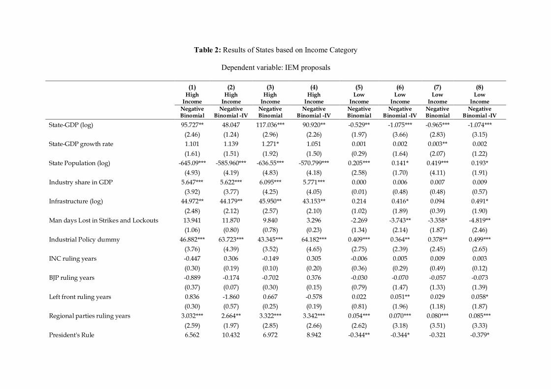
Table 2: Results of States based on Income Category
Dependent variable: IEM proposals
(1) (2) (3) (4) (5) (6) (7) (8) High
Income High
Income High
Income High
Income Low
Income Low
Income Low
Income Low
Income
Negative Binomial
Negative Binomial -IV
Negative Binomial
Negative Binomial -IV
Negative Binomial
Negative Binomial -IV
Negative Binomial
Negative Binomial -IV
State-GDP (log) 95.727** 48.047 117.036*** 90.920** -0.529** -1.075*** -0.965*** -1.074***
(2.46) (1.24) (2.96) (2.26) (1.97) (3.66) (2.83) (3.15)
State-GDP growth rate 1.101 1.139 1.271* 1.051 0.001 0.002 0.003** 0.002
(1.61) (1.51) (1.92) (1.50) (0.29) (1.64) (2.07) (1.22)
State Population (log) -645.09*** -585.960*** -636.55*** -570.799*** 0.205*** 0.141* 0.419*** 0.193*
(4.93) (4.19) (4.83) (4.18) (2.58) (1.70) (4.11) (1.91)
Industry share in GDP 5.647*** 5.622*** 6.095*** 5.771*** 0.000 0.006 0.007 0.009
(3.92) (3.77) (4.25) (4.05) (0.01) (0.48) (0.48) (0.57)
Infrastructure (log) 44.972** 44.179** 45.950** 43.153** 0.214 0.416* 0.094 0.491*
(2.48) (2.12) (2.57) (2.10) (1.02) (1.89) (0.39) (1.90)
Man days Lost in Strikes and Lockouts 13.941 11.870 9.840 3.296 -2.269 -3.743** -3.358* -4.819**
(1.06) (0.80) (0.78) (0.23) (1.34) (2.14) (1.87) (2.46)
Industrial Policy dummy 46.882*** 63.723*** 43.345*** 64.182*** 0.409*** 0.364** 0.378** 0.499***
(3.76) (4.39) (3.52) (4.65) (2.75) (2.39) (2.45) (2.65)
INC ruling years -0.447 0.306 -0.149 0.305 -0.006 0.005 0.009 0.003
(0.30) (0.19) (0.10) (0.20) (0.36) (0.29) (0.49) (0.12)
BJP ruling years -0.889 -0.174 -0.702 0.376 -0.030 -0.070 -0.057 -0.073
(0.37) (0.07) (0.30) (0.15) (0.79) (1.47) (1.33) (1.39)
Left front ruling years 0.836 -1.860 0.667 -0.578 0.022 0.051** 0.029 0.058*
(0.30) (0.57) (0.25) (0.19) (0.81) (1.96) (1.18) (1.87)
Regional parties ruling years 3.032*** 2.664** 3.322*** 3.342*** 0.054*** 0.070*** 0.080*** 0.085***
(2.59) (1.97) (2.85) (2.66) (2.62) (3.18) (3.51) (3.33)
President's Rule 6.562 10.432 6.972 8.942 -0.344** -0.344* -0.321 -0.379*

(0.46) (0.56) (0.48) (0.54) (2.06) (1.83) (1.63) (1.72)
Time trend 0.371 1.638 -3.002 -7.326* 0.044* -0.008 0.044 -0.028
(0.10) (0.45) (0.79) (1.87) (1.86) (0.24) (1.56) (0.69)
Spatial Lag: IEMs High income states 0.399*** 133.641*** 0.326*** 177.412*** 0.0002 0.675*
(8.79) (3.66) (6.52) (4.73) (0.25) (1.69)
Spatial Lag: IEMs Low income states 0.827*** 75.212*** 0.001*** 0.517*** 0.015*** 0.668***
(2.71) (5.03) (2.91) (4.02) (4.28) (4.31)
Log Pseudo likelihood -1862 -1888 -5522 -1879 -566 -562 -556 -561
Goodness-of-fit test (Chi2 statistic) 9340*** 11243*** 8841*** 10399*** 1024*** 1273*** 799*** 1113***
First-stage F-Statistic {using 2-SLS} 32.7*** 47.8***/101.4*** 10.4*** 26.8***/66.5***
Anderson canon LR statistic {using 2-SLS} 101.9*** 298.9*** 46.8*** 190.7***
Hansen J-Statistic (P-value) {using 2-SLS} 0.4721 0.7044 0.032 0.0386
State dummies YES YES YES YES YES YES YES YES
Total states 18 18 18 18 14 14 14 14
Total Observations 334 334 334 334 241 241 241 241
Notes: (a) Robust standard errors in parentheses *** p<0.01, ** p<0.05, * p<0.1
(b) Reports average marginal effects of all explanatory variables

Appendix
Appendix 1: States under study
Andaman & Nicobar Islands Goa Madhya Pradesh Punjab
Andhra Pradesh Gujarat Maharashtra Rajasthan
Arunachal Pradesh Haryana Manipur Sikkim
Assam Himachal Pradesh Meghalaya Tamil Nadu
Bihar Jammu & Kashmir Mizoram Tripura
Chandigarh Jharkhand Nagaland Uttar Pradesh
Chhattisgarh Karnataka Orissa Uttaranchal
Delhi Kerala Pondicherry West Bengal
Appendix 2: Descriptive Statistics
Variables Mean Standard Deviation Minimum Maximum Observations
IEM proposals 131.702 193.542 0.000 1347.000 581
GDP (log) 10.078 1.706 6.092 13.150 594
GDP growth rate 8.134 35.412 -85.115 39.914 591
Population (log) 15.049 1.067 11.567 17.250 592
Industry share in GDP 18.980 11.463 0.651 67.160 594
Infrastructure (log) 6.061 0.815 4.155 7.898 585
Man days lost 0.172 0.556 0.000 5.317 583
Industrial Policy dummy 0.517 0.500 0.000 1.000 584
INC ruling years 2.313 3.445 0.000 16.000 584
BJP ruling years 0.777 2.012 0.000 15.000 584
Left front ruling years 1.113 4.672 0.000 33.000 584
Regional parties ruling years 2.873 6.007 0.000 31.000 584
President's Rule 0.068 0.253 0.000 1.000 584
Spatial lag - IEMs 302.377 80.404 127.208 500.352 579
Spatial lag - IEMs (Predicted values) 5.693 0.190 5.041 6.109 579
Spatial lag (Special category states) 25.319 18.557 3.353 79.356 579
Spatial lag (Non-special category states) 318.965 85.434 136.539 533.890 579
Spatial lag (Special category states PVs) 5.753 0.161 5.128 6.096 579
Spatial lag (Non-special category states PVs) 3.053 0.640 1.052 4.461 579

Appendix 3: Data definitions and sources
Variables Definitions and data sources
IEM approvals IEMs approved from each state in a financial year obtained from SIA, New Delhi
GDP (log) GDP in 1993-94 constant prices (Indian Rupees) from Reserve Bank of India
GDP growth rate Yearly growth rate of GDP from Reserve Bank of India, Mumbai
Population (log) Total population of each state obtained from Indiastat.com
Industry share in GDP Share of Industry in State GDP from Reserve Bank of India, Mumbai
Infrastructure (log) Electricity Consumption in khw by state obtained from Indiastat.com
Man days lost Total man days lost in strikes and lockouts published by Ministry of Labor, Govt. of India
Industrial Policy dummy Own construction based on the information provided by SIA, New Delhi
Political Parties in power Own construction based on the information published by Election Commission of India
President's Rule Own construction based on the information published by Parliament of India
Spatial lag - IEMs Own construction as described in section 3.1
Figure 1: Development of IEM proposals over States during 1991–2009 period
0 200 400 600 800Average IEM proposals per state
West BengalUttaranchal
Uttar PradeshTripura
Tamil NaduSikkim
RajasthanPunjab
PondicherryOrissa
NagalandMizoram
MeghalayaManipur
MaharashtraMadhya Pradesh
KeralaKarnatakaJharkhand
Jammu & KashmirHimachal Pradesh
HaryanaGujarat
GoaDelhi
ChhattisgarhChandigarh
BiharAssam
Arunachal PradeshAndhra Pradesh
Andaman & Nicobar Islands
References Aghion, Philippe, Robin Burgess, Stephen J. Redding and Fabrizio Zilibotti (2008) The Unequal Effects of Liberalization: Evidence from Dismantling the License Raj in India, American Economic Review, 98(4), 1397-1412. Ahmad Ahsan and Carmen Pagés (2009) Are All Labor Regulations Equal? Evidence from Indian Manufacturing, Journal of Comparative Economics, 37, 62-75. Ahluwalia, M.S. (2000) Economic Performance of States in the Post-Reforms Period, Economic and Political Weekly, 1637-1648. Anselin, Luc. (1988) Spatial Econometrics: Methods and Models, Kluwer Academic Publishers: Boston, MA. Aradhna Aggarwal (2007) The Influence of Labour Markets on FDI: Some Empirical Explorations in Export Oriented and Domestic Market Seeking FDI across Indian States, working paper, Delhi University: New Delhi. Arulampalam, Wiji, Sugato Dasgupta, Amrita Dhillon and Bhaskar Dutta (2009) Electoral Goals and Center-State Transfers: A Theoretical Model and Empirical Evidence from India, Journal of Development Economics, 88, 103–119 Asiedu, Elizabeth and Donald Lien (2004) Capital Controls and Foreign Direct Investment, World Development, 32(3), 479–490. Baltagi, Badi H., Peter Egger, and Michael Pfaffermayr (2007) Estimating Models of Complex FDI: Are there Third-Country Effects? Journal of Econometrics, 140(1), 260-281. Basely, Timothy and Robin Burgess (2002) Can Labor Regulation Hinder Economic Performance? Evidence from India, Quarterly Journal of Economics, 19(1), 91-134. Basely, Timothy and Robin Burgess (2000) Land Reform, Poverty Reduction and Growth: Evidence from India, Quarterly Journal of Economics, 115(2), 389-430. Besley, Timothy, Robin Burgess, and Berta Esteve-Volart (2007) The Policy Origins of Poverty and Growth in India, in Delivering on the Promise of Pro-Poor Growth, ed. T. Besley and L. Cord: Palgrave Macmillan and World Bank. Beck, Nathaniel and Jonathan N. Katz, (1995) What To Do (and Not To Do) with Time-Series Cross-Section Data, American Political Science Review, 89(3), 634-647. Beron, Kurt J., James C. Murdoch, and Wim P. M. Vijverberg (2003) Why Cooperate? Public Goods, Economic Power, and the Montreal Protocol, Review of Economics and Statistics, 85(2), 286-297.

Bhagwati, Jagdish (2004) In Defense of Globalization, Princeton: Princeton University. Bhagwati, Jagdish (1999) Globalization: Who Gains, Who Loses?, in: Siebert Horst (ed.), Globalization and Labor, Tubingen: Mohr Siebeck. Biswas, Ringoli and Sugata Marjit (2002) Political Lobbying and Fiscal Federalism: Case of Industrial Licenses and Letters of Intent, Economic and Political Weekly, 37(8), 716-725. Blonigen, Bruce A. (2005) A Review of the Empirical Literature on FDI Determinants, Atlantic Economic Journal, 33(December), 383-403. Blonigen, Bruce A., and David N. Figlio (1998) Voting for Protection: Does Direct Foreign Investment Influence Legislator Behavior? American Economic Review, 88(4), 1002-14. Blonigen, Bruce A., Ronald B. Davies, Glen R. Waddell and Helen Naughton (2007) FDI in Space: Spatial Autoregressive Lags in Foreign Direct Investment, European Economic Review, 51(July), 1303-1325. Blonigen, Bruce A., Ronald B. Davies, Helen T. Naughton, and Glen R. Waddell (2008) Spacey Parents: Autoregressive Patterns in Inbound FDI, in: Foreign Direct Investment and the Multinational Enterprise, Boston: MIT Press. Bound, J., D. Jaeger, and R. Baker (1995) Problems with Instrumental Variables Estimation when the Correlation between the Instruments and the Endogenous Explanatory Variable is Weak, Journal of the American Statistical Association, 90, 443-450. Brandt, Patrick T., John T Williams, Benjamin O. Fordham and Brian Pollins (2000) Dynamic Models for Persistent Event Count Time Series, American Journal of Political Science, 44(4), 823-43. Businessweek (2008) India: Modi Wins as Gujarat Gets Tata's Nano Plant, Accessed on 5thJuly 2011: http://www.businessweek.com/globalbiz/content/oct2008/gb2008108_390634.htm Business Standard (2008) Modi's Gujarat bags Tata's Nano, Accessed on 6thJuly 2011: http://www.business-standard.com/india/news/modis-gujarat-bags-tatas-nano/336735/ Cameron A. C., and Trivedi P. K., (1998) Regression Analysis of Count Data, Cambridge University Press, Cambridge, UK. Cletus C. Coughlin and Eran Segev (2000) Foreign Direct Investment in China: A Spatial Econometric Study, The World Economy, 23(1), 1-23. Chakrabarti, Avik (2001) The Determinants of Foreign Direct Investment: Sensitivity Analyses of Cross-Country Regressions, Kyklos, 54(1), 89-113.
Cho, Seo-Young, Axel Dreher and Eric Neumayer (2011) The Spread of Anti-Trafficking Policies – Evidence from a New Index, Cege Discussion Paper Series No. 119, Georg-August-University of Goettingen, Germany. Cho, Seo-Young (2010) International Human Rights Treaty to Change Social Patterns - The Convention on the Elimination of All forms of Discrimination against Women, CEGE Discussion paper series no.93, Georg-August University Goettingen, Germany. Coughlin, Cletus C., Joseph V. Terza, and Vachira Arromdee (1991) State Characteristics and Location of Foreign Direct Investment within the United States, Review of Economics and Statistics, 73(4), 675-83. Davies, Ronald B. and Krishna Chaitanya Vadlamannati (2011) A Race to the Bottom in Labor Standards? An Empirical Investigation, working paper, University of Heidelberg: Germany. Davies Ronald B. and Johannes Voget (2008) Tax Competition in an Expanding European Union, Working paper 0830, Oxford University Centre for Business Taxation. Davies Ronald B. and Helen T. Naughton (2006) Cooperation in Environmental Policy: A Spatial Approach, Working paper 2006-18, University of Oregon. Davies Ronald B., Hartmut Egger and Peter Egger (2003) Tax Competition for International Producers and the Mode of Foreign Market Entry, Working paper 2006-19, University of Oregon. Devereux, Michael P., Ben Lockwood and Michela Redoano (2008) Do Countries Compete over Corporate Tax Rates? Journal of Public Economics, 92(5-6), 1210-1235. Dreher, Axel, Mikosch, Heiner F. and Voigt, Stefan (2010) Membership Has its Privileges – The Effect of Membership in International Organizations on FDI, CEGE Discussions Paper No. 114, University of Goettingen: Germany. Dreher, Axel and Martin Gassebner (2008) Does Political Proximity to the U.S. Cause Terror?, Economics Letters, 99(1), 27-29. Drusilla K. Brown, Alan Deardorff and Robert Stern (2004) The Effects of Multinational Production on Wages and Working Conditions in Developing Countries, in: Challenges to Globalization: Analyzing the Economics, 279-330 National Bureau of Economic Research. Dunning H. John (1993) Multinational Enterprises and the Global Economy, Wokingham, England: Addision-Wesley. Dutt, Pushan and Devashish Mitra (2006) Labor versus Capital in Trade Policy: The Role of Ideology and Inequality, Journal of International Economics 69(2), 310-20.

Ellingsen, T , and K. Warneryd (1999) Foreign Direct Investment and the Political Economy of Protection, International Economic Review, 40, 357-79. Fredriksson, Per G., John A. List, and Daniel L. Millimet (2004) Chasing the Smokestack: Strategic Policymaking with Multiple Instruments, Regional Science and Urban Economics, 34 (4), 387-410. Fredriksson, Per G., and Daniel L. Millimet (2002) Strategic Interaction and the Determination of Environmental Policy across US States, Journal of Urban Economics, 51, 101-122. Gassebner, Martin, Noel Gaston and Micheal Lamla (2011) The Inverse Domino Effect: Are Economic Reforms Contagious? International Economic Review, 52(1) 183-200. Jakobsen, Jo and Indra de Soysa (2006) Do Foreign Investors punish Democracy? Theory and Empirics, 1984-2001, Kyklos, 55(3), 383-410. Kanta, Murali (2011) Economic Liberalization, Electoral Coalitions and Private Investment in India, paper presented in Politics of FDI Conference, Niehaus Center for Globalization and Governance, September 23-24. Kaushik Basu (2005) Why India Needs Labour Law Reform, BBC report: http://news.bbc.co.uk/2/hi/south_asia/4103554.stm Khemani, Stuti (2007) Does Delegation of Fiscal Policy to an Independent Agency makes a Difference? Evidence from Intergovernmental Transfers in India, Journal of Development Economics, 82, 464–484. King, Gary (1988) Statistical Models for Political Science Event Counts: Bias in Conventional Procedures and Evidence for the Exponential Poisson Regression Model, American Journal of Political Science, 32(3), 838-863. Klemm, Alexander and Stefan van Parys (2009) Empirical Evidence on the Effects of Tax Incentives, Working Paper WP/09/136, IMF: Washington DC. Kobrin, Stephen J. (2005) The Determinants of Liberalization of FDI Policy in Developing Countries: A Cross-Sectional Analysis, 1992-2001, Transnational Corporations, 14(1), 67-104. Kohli, Atul (2004) State-Directed Development: Political Power and Industrialization in the Global Periphery. Cambridge: Cambridge University Press. Kohli, Atul (2006) Politics of Economic Growth in India, 1980-2005, parts I and II, Economic and Political Weekly, 1361-1370. Lawless, J. F., (1987) Negative Binomial and Mixed Poisson Regression, The Canadian Journal of Statistics, 15(3), 209-225.

Levinson, Arik. (2003) Environmental Regulatory Competition: A Status Report and Some New Evidence, National Tax Journal, 56(1), 91-106. Madariaga, Nicole and Sandra Poncet (2007) FDI in Chinese Cities: Spillovers and Impact on Growth, World Economy, 30, 837-862. Markusen, James R., Edward R. Morey and Nancy Olewiler (1995) Competition in Regional Environmental Policies when Plant Locations are Endogenous, Journal of Public Economics, 56(1), 55-77. Murdoch, James C., Todd Sandler, and Wim P. M. Vijverberg (2003) The Participation Decisions versus the Level of Participation in an Environmental Treaty: A Spatial Probit Analysis, Journal of Public Economics, 87, 337-362. Neumayer, Eric and De Soysa, Indra (2011) Globalization and the Empowerment of Women: An Analysis of Spatial Dependence via Trade and FDI, World development, 39(7), 1065-1074. Nunnenkamp, Peter and Megha Mukim (2011a, forthcoming) The Location Choices of Foreign Investors: A District-level Analysis in India, The World Economy. Nunnenkamp, Peter and Megha Mukim (2011b, forthcoming) FDI in India - The Importance of Peer Effects, Applied Economics Letters. Nunnenkamp, Peter and Julius Spatz (2002) Determinants of FDI in Developing Countries: Has Globalization Changed the Rules of the Game?, Transnational Corporations, 11(1), 1-34. Overesch, Michael and Johannes Rincke (2008) Tax Competition in Europe 1980-2007 – Evidence from Dynamic Panel Data Estimation, Working Paper. Perkins, Richard and Neumayer, Eric (2011, forthcoming) Does the ‘California effect’ Operate Across Borders?: Trading and Investing-up in Automobile Emission Standards, Journal of European Public Policy. Pitlik, Hans (2007) A Race to Liberalization? Diffusion of Economic Policy Reform among OECD-Economies, Public Choice, 132, 159–178. Plümper, Thomas and Neumayer, Eric (2010) Model Specification in the Analysis of Spatial Dependence, European Journal of Political Research, 49(3), 418-442 Prakash, Nishith and Aimee Chin (2010) The Redistributive Effects of Political Reservation for Minorities: Evidence from India, NBER Working Paper No. 16509, NBER: Massachusetts. Rudolph, Lloyd I., and Susanne Hoeber Rudolph (2001) Iconisation of Chandrababu: Sharing Sovereignty in India's Federal Market Economy, Economic and Political Weekly, 36(18), 1541-1552.

Schneider, Aaron (2004) Accountability and Capacity in Developing Country Federalism: Empowered States, Competitive Federalism, Forum for Development Studies, 31(1), 33-56. Simmons, BA, Elkins Z, Guzman A. (2006) Competing for Capital: The Diffusion of Bilateral Investment Treaties, 1960-2000, International Organization, 60(4), 811-846. Simmons, BA, Elkins Z. (2004) The Globalization of Liberalization: Policy Diffusion in the International Political Economy, American Political Science Review, 98(1), 171-189. Singh, Nirvikar and Vasishtha, Garima (2004) Patterns in Centre-State Fiscal Transfers: An Illustrative Analysis, Economic and Political Weekly, 39(45), 4897-4903 Srinivasan T. N. (1987) Economic Liberalization in China and India: Issues and an Analytical Framework, Journal of Comparative Economics, 11, 427-443. Staiger, D., and J.H. Stock (1997) Instrumental Variables Regression with Weak Instruments, Econometrica, 65, 557-586. Subramanian, Arvind (2008) India's Turn: Understanding the Economic Transformation, Oxford University Press: UK. Teitelbaum, Emmanuel (2011) Managing Dissent: Government Responses to Industrial Conflict in Post-Reform South Asia. Venkatesan, R. (2000) Study on Policy Competition among States in India for Attracting Direct Investment. New Delhi, India: National Council of Applied Economic Research. Wheeler, David, and Ashoka Mody (1992) International Investment Location Decisions: The Case of U.S. Firms, Journal of International Economics, 33(1-2), 57-76.