A Random Graph Model for Power Law Graphs

William Aiello ∗ Fan Chung †‡ Linyuan Lu §∗

Abstract

We propose a random graph model which is a special case of sparserandom graphs with given degree sequences which satisfy a power law.This model involves only a small number of parameters, called log-size and log-log growth rate. These parameters capture some universalcharacteristics of massive graphs. Furthermore, from these parame-ters, various properties of the graph can be derived. For example, forcertain ranges of the parameters, we will compute the expected distri-bution of the sizes of the connected components which almost surelyoccur with high probability. We will illustrate the consistency of ourmodel with the behavior of some massive graphs derived from data intelecommunications. We will also discuss the threshold function, thegiant component, and the evolution of random graphs in this model.

1 Introduction

Is the World Wide Web completely connected? If not, how big is the largestcomponent, the second largest component, etc.? Anyone who has “surfed”the Web for any length of time will undoubtedly come away feeling that ifthere are disconnected components at all, then they must be small and fewin number. Is the Web too large, dynamic and structureless to answer thesequestions?

Probably yes, if the sizes of the largest components are required to beexact. Recently, however, some structure of the Web has come to light whichmay enable us to describe graph properties of the Web qualitatively. Kumaret al. [13, 14] and Kleinberg et al. [12] have measured the degree sequences ofthe Web and shown that it is well approximated by a power law distribution.

∗AT&T Labs, Florham Park, New Jersey.†University of California, San Diego.‡Research supported in part by NSF Grant No. DMS 98-01446§University of Pennsylvania, Philadelphia.

1

That is, the number of nodes, y, of a given degree x is proportional tox−β for some constant β > 0. This was reported independently by Albert,Barabasi and Jeong in [4, 6, 7]. The power law distribution of the degreesequence appears to be a very robust property of the Web despite its dynamicnature. In fact, the power law distribution of the degree sequence may bea ubiquitous characteristic, applying to many massive real world graphs.Indeed, Abello et al. [1] have shown that the degree sequence of so calledcall graphs is nicely approximated by a power law distribution. Call graphsare graphs of calls handled by some subset of telephony carriers for a specifictime period. In addition, Faloutsos, et al. [10] have shown that the degreesequence of the Internet router graph also follows a power law.

Just as many other real world processes have been effectively modeledby appropriate random models, in this paper we propose a parsimoniousrandom graph model for graphs with a power law degree sequence. Wethen derive connectivity results which hold with high probability in variousregimes of our parameters. And finally, we compare the results from themodel with the exact connectivity structure for some call graphs computedby Abello et al. [1].

An extended abstract of this paper has appeared in the Proceedingsof the Thirtysecond Annual ACM Symposium on Theory of Computing2000 (see [2]). In this paper, we have included the complete proofs forthe main theorems and several additional theorems focused on the secondlargest components of power graphs in various ranges. In addition, somerecent references are provided (also see [11]).

1.1 Power-Law Random Graphs

The study of random graphs dates back to the work of Erdos and Renyiwhose seminal papers [8, 9] laid the foundation for the theory of randomgraphs. There are three standard models for what we will call in this paperuniform random graphs [5]. Each has two parameters. One parameterscontrols the number of nodes in the graph and one controls the density, ornumber of edges. For example, the random graph model G(n, e) assignsuniform probability to all graphs with n nodes and e edges while in therandom graph model G(n, p) each edge is chosen with probability p.

Our power law random graph model also has two parameters. The twoparameters only roughly delineate the size and density but they are naturaland convenient for describing a power law degree sequence. The power lawrandom graph model P (α, β) is described as follows. Let y be the number ofnodes with degree x. P (α, β) assigns uniform probability to all graphs with

2

y = eα/xβ (where self loops are allowed). Note that α is the intercept andβ is the (negative ) slope when the degree sequence is plotted on a log-logscale.

We remark that there is also an alternative power law random graphmodel analogous to the uniform graph model G(n, p). Instead of having afixed degree sequence, the random graph has an expected degree sequencedistribution. The two models are basically asymptotically equivalent, sub-ject to bounding error estimates of the variances (which will be furtherdescribed in a subsequent paper).

1.2 Our Results

Just as for the uniform random graph model where graph properties arestudied for certain regimes of the density parameter and shown to holdwith high probability asymptotically in the size parameter, in this paper westudy the connectivity properties of P (α, β) as a function of the power βwhich hold almost surely for sufficiently large graphs. Briefly, we show thatwhen β < 1, the graph is almost surely connected. For 1 < β < 2 thereis a giant component, i.e., a component of size Θ(n). Moreover, all smallercomponents are of size O(1). For 2 < β < β0 = 3.4785 there is a giantcomponent and all smaller components are of size O(log n). For β = 2 thesmaller components are of size O(log n/ log log n). For β > β0 the graphalmost surely has no giant component. In addition we derive several resultson the sizes of the second largest component. For example, we show thatfor β > 4 the numbers of components of given sizes can be approximated bya power law as well.

1.3 Previous Work

Strictly speaking our model is a special case of random graphs with a givendegree sequence for which there is a large literature. For example, Wormald[20] studied the connectivity of graphs whose degrees are in an interval [r,R],where r ≥ 3. HLuczak [16] considered the asymptotic behavior of the largestcomponent of a random graph with given degree sequence as a functionof the number of vertices of degree 2. His result was further improved byMolloy and Reed [17, 18]. They consider a random graph on n vertices withthe following degree distribution. The number of vertices of degree 0, 1, 2, . . .are about λ0n, λ1n, . . . respectively, where the λ’s sum to 1. It is shown in[17] that if Q =

∑i i(i− 2)λi > 0 and the maximum degree is not too large,

then such random graphs have a giant component with probability tending

3

to 1 as n goes to infinity, while if Q < 0 then all components are smallwith probability tending to 1 as n → ∞. They also examined the thresholdbehavior of such graphs. In this paper, we will apply these techniques todeal with the special case that applies to our model.

Several other papers have taken a different approach to modeling powerlaw graphs than the one taken here [3, 6, 7, 12, 14]. The essential idea of thesepapers is to define a random process for growing a graph by adding nodesand edges. The intent is to show that the defined processes asymptoticallyyield graphs with a power law degree sequence with very high probability.While this approach is interesting and important it has several difficulties.First, the models are difficult to analyze rigorously since the transition prob-abilities are themselves dependent on the the current state. For example,[6, 7] implicitly assume that the probability that a node has a given degreeis a continuous function. The authors of [12, 14] will offer a partial analysisin a recent paper [15]. Second, while the models may generate graphs withpower law degree sequences, it remains to be seen if they generate graphswhich duplicate other structural properties of the Web, the Internet, andcall graphs. For example, the model in [6, 7] cannot generate graphs witha power law other than c/x3. Moreover, all the graphs can be decomposedinto m disjoint trees, wherem is a parameter of the model. The (α, β) modelin [14] is able to generate graphs for which the power law for the indegreeis different than the power law for the outdegree as is the case for the Web.However, to do so, the model requires that there be nodes that have onlyindegree and no outdegree and visa versa. While this may be appropriate forcall graphs (e.g., customer service numbers) it remains to be seen whether itmodels the Web. Thus, while the random graph generation approach holdsthe promise of accurately predicting a wide variety a structural propertiesof many real world massive graphs much work remains to be done.

In this paper we take a different approach. We do not attempt to answerhow a graph comes to have a power law degree sequence. Rather, we takethat as a given. In our model, all graphs with a given power law degreesequence are equi-probable. The goal is to derive structural properties whichhold with probability asymptotically approaching 1. Such an approach,while potentially less accurate than the detailed modelling approach above,has the advantage of being robust: the structural properties derived in thismodel will be true for the vast majority of graphs with the given degreesequence. Thus, we believe that this model will be an important complementto random graph generation models.

We remark that in a subsequent paper[3] several aspects of power lawgraphs are further examined, including (1) analyzing the evolution of graphs,

4

(2) the asymmetry of in-degrees and out-degrees, (3) the “scale invariance”of power law graphs.

The power law random graph model will be described in detail in thenext section. In Sections 3 and 4, our results on connectivity will be derived.In section 5, we discuss the sizes of the second largest components. In section6, we compare the results of our model to exact connectivity data for callgraphs.

2 A random graph model

We consider a random graph with the following degree distribution depend-ing on two given values α and β. Suppose there are y vertices of degree xwhere x and y satisfy

log y = α− β log x

In other words, we have

| v : deg(v) = x |= y =eα

xβ

Basically, α is the logarithm of the size of the graph and β can be regardedas the log-log growth rate of the graph.

We note that the number of edges should be an integer. To be precise,the above expression for y should be rounded down to eα

xβ . If we use realnumbers instead of rounding down to integers, it may cause some error termsin further computation. However, we will see that the error terms can beeasily bounded. For simplicity and convenience, we will use real numberswith the understanding the actual numbers are their integer parts. Anotherconstraint is that the sum of the degrees should be even. This can be assuredby adding a vertex of degree 1 if the sum is old if needed. Furthermore, forsimplicity, we here assume that there is no isolated vertices.

We can deduce the following facts for our graph:(1) The maximum degree of the graph is e

αβ . Note that 0 ≤ log y = α −

β log x.(2) The vertices number n can be computed as follows: By summing y(x)for x from 1 to e

αβ , we have

n =e

αβ∑

x=1

eα

xβ≈

ζ(β)eα if β > 1αeα if β = 1e

αβ

1−β if 0 < β < 1

5

where ζ(t) =∑∞

n=11nt is the Riemann Zeta function.

(3) The number of edges E can be computed as follows:

E =12

eαβ∑

x=1

xeα

xβ≈

12ζ(β − 1)eα if β > 214αe

α if β = 212

e2αβ

2−β if 0 < β < 2

(4) The differences of the real numbers in (1)-(3) and their integer parts canbe estimated as follows: For the number n of vertices, the error term is atmost e

αβ . For β ≥ 1, it is o(n), which is a lower order term. For 0 < β < 1,

the error term for n is relatively large. In this case, we have

n ≥ eαβ

1− β− e

αβ =

βeαβ

1− β

Therefore, n has the same magnitude as eαβ

1−β . The number E of edges canbe treated in a similarly way. For β ≥ 2, the error term of E is o(E), alower order term. For 0 < β < 2, E has the same magnitude as in formulaof item (3). In this paper, we mainly deal with the case β > 2. The onlyplace that we deal with the case 0 < β < 2 is in the next section wherewe refer to 2− β as a constant. By using real numbers instead of roundingdown to their integer parts, we simplify the arguments without affecting theconclusions.

In order to consider the random graph model, we will need to considerlarge n. We say that some property almost surely (a. s. ) happens if theprobability that the property holds tends to 1 as the number n of the verticesgoes to infinity. Thus we consider α to be large but where β is fixed.

We use the following random graph model for a given degree sequence:The model:1. Form a set L containing deg(v) distinct copies of each vertex v.2. Choose a random matching of the elements of L.3. For two vertices u and v, the number of edges joining u and v is equalto the number of edges in the matching of L joining copies of u to copies ofv.

We remark that the graphs that we are considering are in fact multi-graphs, possibly with loops. This model is a natural extension of the modelfor k-regular graphs, which is formed by combining k random matching. Forreferences and undefined terminology, the reader is referred to [5, 21].

We note that this random graph model is slightly different from theuniform selection model P (α, β) as described in section 1.1. However, by

6

using techniques in Lemma 1 of [18], it can be shown that if a random graphwith a given degree sequence a. s. has property P under one of these twomodels, then it a. s. has property P under the other model, provided somegeneral conditions are satisfied.

3 The connected components

Molloy and Reed [17] showed that for a random graph with (λi + o(1))nvertices of degree i, where λi are non-negative values which sum to 1, thegiant component emerges when Q =

∑i≥1 i(i− 2)λi > 0, provided that the

maximum degree is less than n1/4−ε. They also show that almost surelythere is no giant component when Q =

∑i≥1 i(i − 2)λi < 0 and maximum

degree less than n1/8−ε.Here we compute Q for our (α, β)-graphs.

Q =e

αβ∑

x=1

x(x− 2) eα

xβ

≈e

αβ∑

x=1

eα

xβ−2− 2

eαβ∑

x=1

eα

xβ−1

≈ (ζ(β − 2)− 2ζ(β − 1))eα if β > 3

Hence, we consider the value β0 = 3.47875 . . ., which is a solution to

ζ(β − 2)− 2ζ(β − 1) = 0

If β > β0, we havee

αβ∑

x=1

x(x− 2) eα

xβ < 0

We first summarize the results here:

1. When β > β0 = 3.47875 . . ., the random graph a. s. has no giantcomponent. When β < β0 = 3.47875 . . ., there is a. s. a unique giantcomponent.

2. When 2 < β < β0 = 3.47875 . . ., the second largest components area. s. of size Θ(log n). For any 2 ≤ x < Θ(log n), there is almost surelya component of size x.

7

3. When β = 2, a. s. the second largest components are of size Θ( log nloglog n).

For any 2 ≤ x < Θ( log nloglog n), there is almost surely a component of size

x.

4. When 1 < β < 2, the second largest components are a. s. of size Θ(1).The graph is a. s. not connected.

5. When 0 < β < 1, the graph is a. s. connected.

6. For β = β0 = 3.47875 . . ., this is a very complicated case. It corre-sponds to the double jump of random graph G(n, p) with p = 1

n . Forβ = 1, there is a nontrivial probability for either cases that the graphis connected or disconnected.

We remark that for β > 8, Molloy and Reed’s result immediately impliesthat almost surely there is no giant component. When β ≤ 8, additionalanalysis is needed to deal with the degree constraints. We will prove inTheorem 2 that almost surely there is no giant component when β > β0. Insection 5, we will deal with the range β < β0. We will show in Theorem 3that almost surely there is a unique giant component when β < β0. Fur-thermore, we will determine the size of the second largest component withina constant factor.

4 The sizes of connected components in certainranges for β

For β > β0 = 3.47875 . . ., almost surely there is no giant component. Thisrange is of special interest since it is quite useful later for describing thedistribution of small components. We will prove the following:

Theorem 1 For (α, β)-graphs with β > 4, the distribution of the numberof connected components is as follows:

1. For each vertex v of degree d = Ω(1), let τ be the size of connectedcomponent containing v. Then

Pr(|τ − d

c1| > 2λ

c1

√dc2c1

) ≤ 2λ2

where λ = dε. In other words, the vertex v a. s. belongs to a connectedcomponent of size d

c1+O(d

12+ε), where c1 = 2− ζ(β−2)

ζ(β−1) , c2 = ζ(β−3)ζ(β−1) −

8

(ζ(β−2)ζ(β−1)

)2are two constants, ε is an arbitrary small positive number

and d is a (slowly) increasing function of n.

2. The number of connected components of size x is a. s. at least

(1 + o(1))eα

cβ−11 xβ

.

and at most

c3eα log

β2−1 n

xβ2+1

where c3 = 41+βc2(β−2)c1+β

1

is a constant only depending on β.

3. A connected component of the (α, β)-graph a. s. has the size at most

e2α

β+2α = Θ(n2

β+2 log n)

In our proof we use the second moment whose convergence depends on β > 4.In fact for β ≤ 4 the second moment diverges as the size of the graph goesto infinity so that our method no longer applies.

Theorem 1 strengthens the following result (which can be derived fromLemma 3 in [17]) for the range of β > 4.

Theorem 2 For β > β0 = 3.47875 . . ., a connected component of the (α, β)-graph a. s. has the size at most

Ce2αβ α = Θ(n

2β log n)

where C = 16c21

is a constant only depending on β.

The proof for Theorem 2 is by using branching process method. We herebriefly describe the proof since it is needed for the proof of Theorem 1. Pickany vertex v in our graph, expose its neighbors, and then the neighbors of itsneighbors, repeating until the entire component is exposed. We expose onlyone vertex at each stage. At stage i, let Li be the set of vertices exposedand Xi be the random variable that counts the number of vertices in Li.We mark all vertices in Li by either “live” or “dead”. A vertex in Li, whoseneighbors have not been all exposed yet, is marked “live”. A vertex, whoseneighbors have all been exposed, is marked “dead”. Let Oi be the set oflive vertices and Yi be the random variable that is the number of vertices

9

in Oi. Each step we mark exact one dead vertex, so the total number ofdead vertices at i-th step is i. We have Xi = Yi + i. Initially we assignL0 = O0 = v. Then at stage i ≥ 1, we do the following:

1. If Yi−1 = 0, then we stop and output Xi−1.

2. Otherwise, randomly choose a live vertex u from Oi−1 and exposeits neighbors in Nu. Then mark u dead and mark each vertex liveif it is in Nu but not in Li−1. We have Li = Li−1 ∪ Nu, and Oi =(Oi−1 \ u) ∪ (Nu \ Li−1).

Suppose that v has degree d. Then X1 = d+ 1, and Y1 = d. EventuallyYi will hit 0 if i is large enough. Let τ denote the stopping time of Y ,namely, Yτ = 0. Then Xτ = Yτ + τ = τ measures the size of the connectedcomponent. We first compute the expected value of Yi and then use Azuma’sInequality [17] to prove Theorem 2.

Suppose that the vertex u is exposed at stage i. Then Nu∩Li−1 containsat least one vertex v, which was exposed to reach u. However, Nu ∩ Li−1

may contain more than one vertex. We call an edge from u to Li−1 (that isnot v) a “backedge”. We note that “backedges” causes the exploration tostop more quickly, especially when the component is large. However in ourcase β > β0 = 3.47875 . . ., the contribution of “backedges” is quite small.We denote Zi = #Nu and Wi = #Nu ∩ Li−1 − 1. Zi measures thedegree of the vertex exposed at stage i, while Wi measures the number of“backedges”. By definition, we have

Yi − Yi−1 = Zi − 2−Wi.

We have

E(Zi) =∑e

αβ

x=1 xx eα

xβ

E = eα

E

∑eαβ

x=1 x2−β

= ζ(β−2)+O(n3β−1

)

ζ(β−1)+O(n2β−1

)

= ζ(β−2)ζ(β−1) +O(n

3β−1)

Now we will bound Wi. Suppose that there are m edges exposed at stagei−1. Then the probability that a new neighbor is in Li−1 is at most m

E . Wehave

E(Wi) ≤∞∑

x=1

x(mE

)x

10

=mE

(1− mE )2

(∗)

=m

E+O((

m

E)2)

provided mE = o(1).

When i ≤ Ce2αβ α, m is at most ie

αβ ≤ Ce

3αβ α. Hence,

m

E= O(n

3β−1 log n) = o(1)

We have

E(Yi) = Y1 +i∑

j=2

E(Yj − Yj−1)

= d+i∑

j=2

E(Zj − 2−Wj)

= d+ (i− 1)(ζ(β − 2)ζ(β − 1)

− 2)− iO(n

3β−1 log n)

= d− c1(i− 1) + io(1)

Proof of Theorem 2: Since |Yj − Yj−1| ≤ eαβ , by Azuma’s martingale

inequality, we have

Pr(|Yi − E(Yi)| > t) ≤ 2e−t2

2ie2αβ

where i = 16c21e

2αβ log n, and t = c1

2 i. Since

E(Yi) + t = d− c1(i− 1) + io(1) +c12i = −c1

2i+ d+ c1 + io(1) < 0

We have

Pr(τ > 16c21e

αβ log n) = Pr(τ > i) ≤ Pr(Yi ≥ 0)

≤ Pr(Yi > E(Yi) + t)

≤ 2e−t2

2ie2αβ = 2

n2

Hence, the probability that there exists a vertex v such that v lies in acomponent of size greater than 16

c21e

2αβ log n is at most

n2n2

=2n

= o(1).

11

The proof of Theorem 1 uses the methodology above as a starting pointwhile introducing the calculation of the variance of the above random vari-ables.Proof of Theorem 1

We follow the notation and previous results of Section 4. Under theassumption β > 4, we consider the following:

V ar(Zi) =e

αβ∑

x=1

x2x eα

xβ

E− E(Zi)2

=eα

E

eαβ∑

x=1

x3−β − E(Zi)2

=ζ(β − 3) +O(n

4β−1)

ζ(β − 1) +O(n2β−1)

−(ζ(β − 2)ζ(β − 1)

)2

+O(n3β−1)

=ζ(β − 3)ζ(β − 1)

−(ζ(β − 2)ζ(β − 1)

)2

+O(n4β−1)

= c2 + o(1)

since β > 4.We need to compute the covariants. There are models for random graphs

in which the edges are in dependently chosen. Then, Zi and Zj are indepen-dent. However, in the model based on random matchings, there is a smallcorrelation. For example, Zi = x slightly effects the probability of Zj = y.Namely, Zj = x has slightly less chance, while Zj = y = x has slightly morechance. Both differences can be bounded by

1E − 1

− 1E

≤ 2E2

Hence CoV ar(Zi, Zj) ≤ E(Zi)E 2E2 = O( 1

n) if i = j.Now we will bound Wi. Suppose that there are m edges exposed at stage

i−1. Then the probability that a new neighbor is in Li−1 is at most mE . We

have

V ar(Wi) ≤∞∑

x=1

x3(mE

)x − E(Wi)2

=mE (m

E + 1)(1− m

E )3−O((

m

E)2)

12

=m

E+O((

m

E)2)

CoV ar(Wi,Wj) ≤√V ar(Wi)V ar(Wj) ≤ m

E+O((

m

E)2)

CoV ar(Zi,Wj) ≤√V ar(Zi)V ar(Wj) = O(

√m

E)

When i = O(eαβ ), m ≤ ie

αβ = O(e

2αβ ), we have

E(Yi) = d+ (i− 1)(ζ(β − 2)ζ(β − 1)

− 2)

+ iO(n3β−1) + i

m

E

= d− (i− 1)c1 +O(n4β−1)

= d− (i− 1)c1 + o(1)

V ar(Yi) = V ar(d+i∑

j=2

(Yj − Yj−1))

= V ar(i∑

j=2

(Zj −Wj))

=i∑

j=2

(V ar(Zj) + V ar(Wj))

+∑

2≤j =k≤i

(CoV ar(Zj , Zk)

−CoV ar(Zj,Wk) + CoV ar(Wj ,Wk))

= ic2 + io(1) + i2(O(1n) +O(

√e( 2

β−1)α)

+O(e( 2β−1)α))

= ic2 + io(1) + i(O(e( 2β− 1

2)α) +O(e( 3

β−1)α))

= ic2 + io(1)

Chebyshev’s inequality gives

Pr(|Yi −E(Yi)| > λσ) <1λ2

where σ is the standard deviation of Yi, σ =√ic2 + o(

√i) Let i1 = d

c1−

2λc1

√dc2c1

and i2 = dc1

+ 2λc1

√dc2c1

. We have

E(Yi1)− λσ = d− (i1 − 1)c1 + o(1)− (λ√c2i1 + o(√i1))

13

≥ 2λ√

dc2c1

− λ

√c2

d

c1− o(

√d)

= λ

√dc2c1

− o(√d)

> 0

Hence,

Pr(τ < i1) ≤ Pr(Yi1 ≤ 0) ≤ Pr(Yi1 < E(Yi1)− λσ) ≤ 1λ2

Similarly,

E(Yi2) + λσ = d− (i2 − 1)c1 + o(1) +(λ√c2i2 + o(

√i2))

≥ −2λ√

dc2c1

+ λ

√c2

d

c1+ o(

√d)

= −λ

√dc2c1

+ o(√d)

< 0

Hence,

Pr(τ > i2) ≤ Pr(Yi2 > 0) ≤ Pr(Yi2 > E(Yi2) + λσ) ≤ 1λ2

Therefore

Pr(|τ − d

c1| > 2λ

c1

√dc2c1

) ≤ 2λ2

For a fixed v and λ a slowly increasing function to infinity, above inequalityimplies that almost surely we have τ = d

c1+O(λ

√d).

We note that almost all components generated by vertices of degree xis about the size of d

c1. One such component can have at most about 1

c1

vertices of degree d. Hence, the number of component of size dc1

is at leastc1e

αβ

dβ . Let d = c1x. Then the number of components of size x is at least

eαβ

cβ−11 xβ

(1 + o(1))

The proof above actually gives the following result. The size of every com-ponent, whose vertices have degree at most d0, is almost surely Cd2

0 log nwhere C = 16

c21is the same constant as in Theorem 2. Let x = Cd2

0 log n and

14

consider the number of components of size x. A component of size x almostsurely contains at least one vertex of degree greater than d0.

For each vertex v with degree d ≥ d0, by part 1 in the statement ofTheorem 1, we have

Pr

(|τ − d

c1| > 2λd

c1

√dc2c1

)≤ 2

λ2d

Let λd = c1Cd20 log n4

√c1c2d , we have

Pr(τ ≥ Cd20 log n) ≤ Pr

(τ >

d

c1+

2λd

c1

√dc2c1

)

≤ C3d

d40 log

2 n

where C3 = 32c2c31C2 = c1c2

8 is constant depending only on β. Since there are

only eα

dβ vertices of degree d, the number of components of size at least x isat most

eαβ∑

d=d0

eα

dβC3

d

d40 log

2 n≤ C3e

α

d40 log

2 n

∞∑d=d0

1dβ−1

≤ C3eα

d40 log

2 n

2β − 2

1

dβ−20

=2C3e

α

(β − 2)dβ+20 log2 n

= c3eα log

β2−1 n

xβ2+1

where c3 = 2C3(β−2)C

1+ β2 = 41+βc2

(β−2)c1+β1

. For x = e2α

β+2α, the above inequality

implies that the number of components of size at least x is at most o(1). Inother words, almost surely no component has size greater than e

2αβ+2α. This

completes the proof of Theorem 1.

5 On the size of the second largest component

For β < β0 = 3.47875 . . ., we consider the giant component as well as thesize of the second largest component.

15

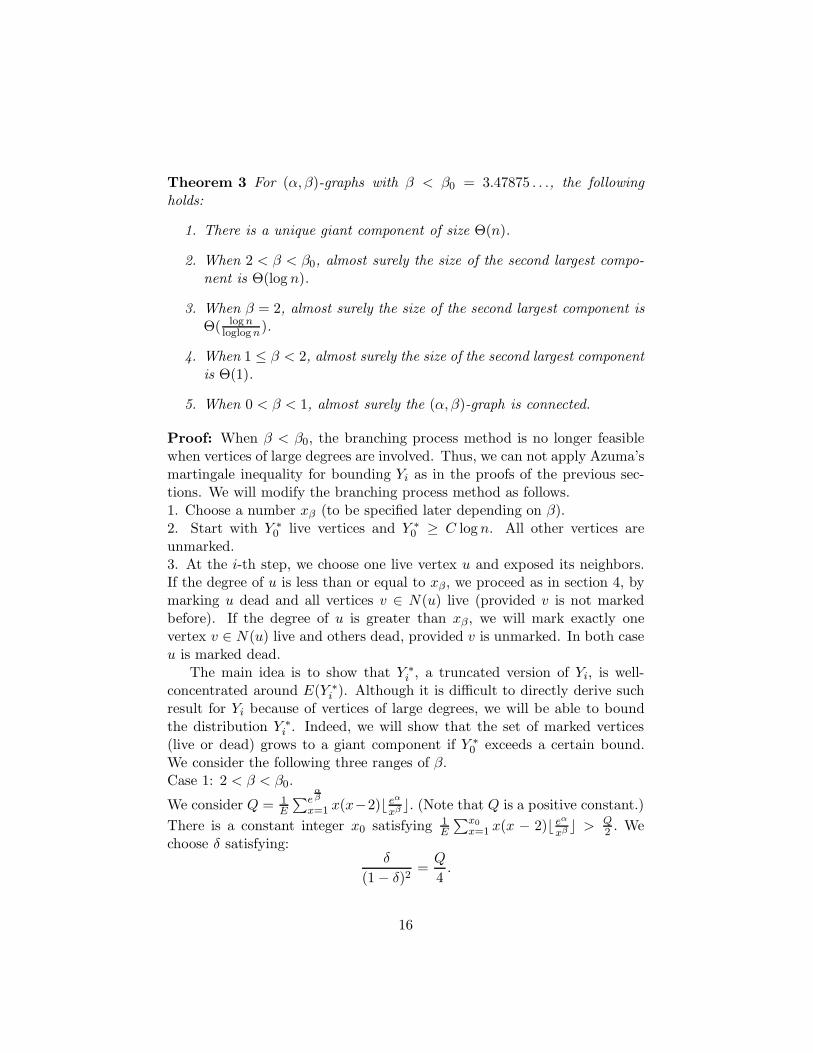
Theorem 3 For (α, β)-graphs with β < β0 = 3.47875 . . ., the followingholds:

1. There is a unique giant component of size Θ(n).

2. When 2 < β < β0, almost surely the size of the second largest compo-nent is Θ(log n).

3. When β = 2, almost surely the size of the second largest component isΘ( log n

loglog n).

4. When 1 ≤ β < 2, almost surely the size of the second largest componentis Θ(1).

5. When 0 < β < 1, almost surely the (α, β)-graph is connected.

Proof: When β < β0, the branching process method is no longer feasiblewhen vertices of large degrees are involved. Thus, we can not apply Azuma’smartingale inequality for bounding Yi as in the proofs of the previous sec-tions. We will modify the branching process method as follows.1. Choose a number xβ (to be specified later depending on β).2. Start with Y ∗

0 live vertices and Y ∗0 ≥ C log n. All other vertices are

unmarked.3. At the i-th step, we choose one live vertex u and exposed its neighbors.If the degree of u is less than or equal to xβ, we proceed as in section 4, bymarking u dead and all vertices v ∈ N(u) live (provided v is not markedbefore). If the degree of u is greater than xβ, we will mark exactly onevertex v ∈ N(u) live and others dead, provided v is unmarked. In both caseu is marked dead.

The main idea is to show that Y ∗i , a truncated version of Yi, is well-

concentrated around E(Y ∗i ). Although it is difficult to directly derive such

result for Yi because of vertices of large degrees, we will be able to boundthe distribution Y ∗

i . Indeed, we will show that the set of marked vertices(live or dead) grows to a giant component if Y ∗

0 exceeds a certain bound.We consider the following three ranges of β.Case 1: 2 < β < β0.

We consider Q = 1E

∑eαβ

x=1 x(x−2) eα

xβ . (Note that Q is a positive constant.)There is a constant integer x0 satisfying 1

E

∑x0x=1 x(x − 2) eα

xβ > Q2 . We

choose δ satisfying:δ

(1− δ)2=

Q

4.

16

If the component has more than δE edges, it must have Θ(n) vertices sinceβ > 2. So it is a giant component and we are done. We may assume thatthe component has no more than δE edges.

We now choose xβ = x0 and apply the modified branching process. Then,Y ∗

i satisfies the following:

• Y ∗0 ≥ C log n, where C = 130x2

0Q is a constant only depending on β.

• −1 ≤ Y ∗i − Y ∗

i−1 ≤ x0.

• Let Wi be the number of “backedges” as defined in section 4. Byinequality (*) and the assumption that the number of edges m in thecomponent is at most δn, we have E(Wi) ≤ δ

(1−δ)2= Q

4 . Hence, wehave

E(Y ∗i − Y ∗

i−1) ≈ 1E

x0∑x=1

x(x− 2) eα

xβ − E(Wi)

≥ Q

2− Q

4=

Q

4.

By Azuma’s martingale inequality, we have

Pr(Y ∗i ≤ Qi

8) ≤ Pr(Y ∗

i − E(Y ∗i ) ≤ −Qi

8)

< e− (Qi/8)2

2ix20 = o(n−1)

provided i > C log n.The above inequality implies that with probability at least 1 − o(n−1),

Y ∗i > Qi

8 > 0 when i > C log n. Since Y ∗i decreases at most by 1 at each

step, Y ∗i can not be zero if i ≤ C log n. So Y ∗

i > 0 for all i. In other words,a. s. the branching process will not stop. However, it is impossible to haveY ∗

n > 0, that is a contradiction. Thus we conclude that the componentmust have at least δn edges. So it is a giant component. We note that if acomponent has more than C log n edges exposed, then almost surely it is agiant component. In particular, any vertex with degree more than C log nis almost surely in the giant component. Hence, the second component havesize of at most Θ(log n).

Next, we will show that the second largest has size at least Θ(log n). Weconsider the vertices v of degree x = cα, where c is some constant. Thereis a positive probability that all neighboring vertices of v have degree 1.

17

In this case, we get a connected component of size x + 1 = Θ(log n). Theprobability of this is about

(1

ζ(β − 1))cα

Since there are eα

(cα)β vertices of degree x, the probability that none of themhas the above property is about

(1− 1ζ(β − 1)cα

)eα

(cα)β ≈ e− 1

ζ(β−1)cαeα

(cα)β

= e−

( eζ(β−1)c

)α

(cα)β = o(1)

where we have

c =

1 if β ≥ 31

−2 log(β−2) if 3 > β > 2

In other words, a. s. there is a component of size cα + 1 = Θ(log n).Therefore, the second largest component has size Θ(log n). Moreover, theabove argument holds if we replace cα by any small number. Hence, smallcomponents exhibit a continuous behavior.Case 2: β = 2.We choose xβ = 10α. We note that a component with more than 2E/3 edgesmust be unique. We will prove that almost surely the unique componentcontains all vertices with degree greater than 101α2. So it contains (1 −o(1))E edges and it is the giant component.

We further modify the branching process by starting from Y ∗0 ≥ 101α2

vertices. If the component has more than 2E/3 edges, we are done. Other-wise, the expected number of backeges is small.

E(Wi) ≤ 2/3(1− 2/3)2

= 6

from inequality (*). Hence, Y ∗i satisfies:

• Y ∗0 ≥ 101α2.

• −1 ≤ Y ∗i − Y ∗

i−1 ≤ 10α.

• E(Y ∗i − Y ∗

i−1) ≈ 1E

∑10αx=1 x(x− 2) eα

xβ −E(Wi)> 10− 2− 6 = 2

18

By Azuma’s martingale inequality, we have

Pr(Y ∗i ≤ i) ≤ Pr(Y ∗

i − E(Y ∗i ) ≤ −i

< e− i2

i(10α)2 = o(n−1)

provided i ≥ 101α2.The above inequality implies that with proability at least 1 − o(n−1),

Y ∗i ≥ i > 0 when i > 101α2. Since Y ∗

i decreases at most by 1 at eachstep, Y ∗

i can not be zero if i ≤ 101α2. So Y ∗i > 0 for all i. In other words,

a. s. the branching process will not stop. However, it is impossible to haveY ∗

n > 0, that is a contradiction. Thus we conclude that the component musthave at least 2

3E edges. We note that a. s. all vertices with degree morethan 101α2 are in the unique component with at least 2

3E edges, hencethe giant component.

The probability that a random vertex is in the giant component is atmost

1E

101α2∑x=1

xeα

x2≈ 2 log α

α

The probability that there are 2.1 αlog α vertices not in the giant component

is at most(2 log α

α)2.1 α

log α = e−(2.1+o(1))α = o(n−2).

Since there is at most n connected components, we conclude that a. s. aconnected component of size greater that 2.1 α

log α = Θ( log nloglog n) must be the

giant component.Now we find a vertex v of degree x and x ≤ 0.9 α

log α . The probabilitythat all its neighbors are of degree 1 is ( 1

α)x. The probability that no such

vertex exists is at most

(1− (1α)x)

eα

x2 ≈ e−( 1α

)x eα

x2 = e−e0.1α

x2 = o(1)

Hence, a. s. there is a vertex of degree x ≤ 0.9 αlog α , which forms a connected

component of size x+1. This proves that a. s. the second largest componenthas size Θ( log n

loglog n).Case 3: 0 < β < 2.

We use the modified branching process by choosing xβ = e(5−2β)α(6−2β)β . If a

component has more than 2E/3 edges, it is the unqiue giant componentand we are done. Otherwise, we have

E(Wi) ≤ 2/3(1− 2/3)2

= 6.

19

Hence, Y ∗i satisfies:

• Y ∗0 ≥ 5

C2 e(2−β)α(3−β)β .

• −1 ≤ Y ∗i − Y ∗

i−1 ≤ e(5−2β)α(6−2β)β .

• E(Y ∗i − Y ∗

i−1) ≈ 1E

∑e(5−2β)α(6−2β)β

x=1 x(x− 2) eα

xβ − E(Wi)≈ Ce

α2β

Here C is a constant depending only on β.By Azuma’s martingale inequality, we have

Pr(Y ∗i ≤ 1

2Ce

α2β i) < Pr(Y ∗

i − E(Y ∗i ) ≤ −1

2Ce

α2β i)

< e− ( 1

2 Ceα2β i)2

i(e((5−2β)α)/((6−2β)β))2 = o(n−1)

provided i ≥ 5C2 e

(2−β)α(3−β)β .

The above inequality shows that with probability at least 1 − o(n−1),

Y ∗i > 1

2Ceα2β i > 0 provided i > 5

C2 e(2−β)α(3−β)β . Since Y ∗

i decreases at most by

1 at each step, Y ∗i can not be zero if i ≤ 5

C2 e(2−β)α(3−β)β . So Y ∗

i > 0 for all i.In othe words, a. s. the branching processing will not stop. However, it isimpossible to have Y ∗

n > 0, that is a contradiction. So, a. s. all vertices with

degree more than 5C2 e

(2−β)α(3−β)β are in the giant component. The probability

that a random vertex is in the giant component is at most

1E

5C2 e

(2−β)α(3−β)β∑

x=1

xeα

xβ= Θ(e−

(2−β)α(3−β)β )

The probability that all 23−β2−β +1 vertices are not in the giant vertex is at

most(Θ(e−

(2−β)α(3−β)β ))2

3−β2−β

+1 = o(n−2).

Since there is at most n connected component, we conclude that a. s. aconnected component of size greater that 23−β

2−β = Θ(1) must be the giantcomponent.

For 1 < β < 2, we fix a vertex v of degree 1. The probability that theother vertex that connects to v is also of degree 1 is

Θ(eα

e2αβ

)

20

Therefore the probability that no component has size of 2 is at most

(1−Θ(eα

e2αβ

))eα ≈ e−Θ(e

2α− 2αβ ) ≈ o(1)

In other words, the graph a. s. has at least one component of size 2.For 0 < β < 1, we want to show that the random graph is a. s. con-

nected. Since the size of the possible second largest component is boundedby a constant M , all vertices of degree ≥ M are almost surely in the giantcomponent. We only need to show the probability that there is an edgeconnecting two small degree vertices is small. There are only

M∑x=1

x eα

xβ ≈ Ceα

vertices with degree less than M . For any random pair of vertices (u, v), theprobability that there is an edges connecting them is about

1E

= Θ(e−2αβ )

Hence the probability that there is edge connecting two small degree verticesis at most ∑

u,v

1E

= (Ceα)2Θ(e2αβ ) = o(1)

Hence, every vertex is a. s. connected to a vertex with degree ≥ M , whicha. s. belongs to the giant exponent. Hence, the random graph is a. s.connected.

6 Comparisons with realistic massive graphs

Our (α, β)-random graph model was originally derived from massive graphsgenerated by long distance telephone calls. These so-called call graphs aretaken over different time intervals. For the sake of simplicity, we considerall the calls made in one day. Every completed phone call is an edge in thegraph. Every phone number which either originates or receives a call is anode in the graph. When a node originates a call, the edge is directed out ofthe node and contributes to that node’s outdegree. Likewise, when a nodereceives a call, the edge is directed into the node and contributes to thatnode’s indegree.

21

In Figure 2, we plot the number of vertices versus the indegree for the callgraph of a particular day. Let y(i) be the number of vertices with indegreei . For each i such that y(i) > 0, a × is marked at the coordinate (i , y(i)).As similar plot is shown in Figure 1 for the outdegree. Plots of the numberof vertices versus the indegree or outdegree for the call graphs of other daysare very similar. For the same call graph in Figure 3 we plot the number ofconnected components for each possible size.

The degree sequence of the call graph does not obey perfectly the (α, β)-graph model. The number of vertices of a given degree does not evenmonotonically decrease with increasing degree. Moreover, the call graphis directed, i.e., for each edge there is a node that originates the call and anode that receives the call. The indegree and outdegree of a node need notbe the same. Clearly the (α, β)-random graph model does not capture allof the random behavior of the real world call graph.

Nonetheless, our model does capture some of the behavior of the callgraph. To see this we first estimate α and β of Figure 2. Recall that foran (α, β)-graph, the number of vertices as a function of degree is given bylog y = α− β log x. By approximating Figure 2 by a straight line, β can beestimated using the slope of the line to be approximately 2.1. The value ofeα for Figure 2 is approximately 30× 106. The total number of nodes in thecall graph can be estimated by ζ(2.1) ∗ eα = 1.56 ∗ eα ≈ 47× 106

For β between 2 and β0, the (α, β)-graph will have a giant componentof size Θ(n). In addition, a. s. , all other components are of size O(log n).Moreover, for any 2 ≥ x ≥ O(log n), a component of size x exists. This isqualitatively true of the distribution of component sizes of the call graphin Figure 31. The one giant component contains nearly all of the nodes.The maximum size of the next largest component is indeed exponentiallysmaller than the size of the giant component. Also, a component of nearlyevery size below this maximum exists. Interestingly, the distribution of thenumber of components of size smaller than the giant component is nearlylog-log linear. This suggests that after removing the giant component, oneis left with an (α, β)-graph with β > 4 (Theorem 1 yields a log-log linearrelation between number of components and component size for β > 4. )This intuitively seems true since the greater the degree, the fewer nodes ofthat degree we expect to remain after deleting the giant component. Thiswill increase the value of β for the resulting graph.

1This data was compiled by J. Abello and A. Buchsbaum of AT&T Labs from rawphone call records using, in part, the external memory algorithm of Abello, Buchsbaum,and Westbrook [1] for computing connected components of massive graphs.

22

There are numerous questions that remain to be studied. For example,what is the effect of time scaling? How does it correspond with the evolutionof β? What are the structural behaviors of the call graphs? What are thecorrelations between the directed and undirected graphs? It is of interestto understand the phase transition of the giant component in the realisticgraph. In the other direction, the number of tiny components of size 1 isleading to many interesting questions as well. Clearly, there is much workto be done in our understanding of massive graphs.

Acknowledgments. We are grateful to J. Feigenbaum, J. Abello, A. Buchs-baum, J. Reeds, and J. Westbrook for their assistance in preparing thefigures and for many interesting discussions on call graphs. We are verythankful to the anonymous referees for their invaluable comments.

References

[1] J. Abello, A. Buchsbaum, and J. Westbrook, A functional approach to externalgraph algorithms, Proc. 6th European Symposium on Algorithms, pp. 332–343,1998.

[2] W. Aiello, F. Chung, L. Lu, A random graph model for massive graphs, Pro-ceedings of the Thirtysecond Annual ACM Symposium on Theory of Comput-ing, (2000), 171-180.

[3] W. Aiello, F. Chung, L. Lu, Random evolution of power law graphs, Handbookof Massive Data Sets, Vol. 2, (eds. J. Abello et al.), to appear.

[4] R. Albert, H. Jeong and A. Barabasi, Diameter of the World Wide Web,Nature, 401, September 9, 1999.

[5] N. Alon and J. H. Spencer, The Probabilistic Method, Wiley and Sons, NewYork, 1992.

[6] A. Barabasi, and R. Albert, Emergence of scaling in random networks, Science,286, October 15, 1999.

[7] A. Barabasi, R. Albert, and H. Jeong Scale-free characteristics of randomnetworks: the topology of the world wide web, Elsevier Preprint August 6,1999.

[8] P. Erdos and A. Renyi, On the evolution of random graphs, Publ. Math. Inst.Hung. Acad. Sci. 5 (1960), 17–61.

[9] P. Erdos and A. Renyi, On the strength of connectedness of random graphs,Acta Math. Acad. Sci. Hungar. 12 (1961), 261-267.

23

[10] M. Faloutsos, P. Faloutsos, and C. Faloutsos, On power-law relationships of theinternet topology, Proceedings of the ACM SIGCOM Conference, Cambridge,MA, 1999.

[11] Brian Hayes, Graph theory in practice: Part II, American Scientists, 88,(March-April, 2000), 104-109.

[12] J. Kleinberg, S. R. Kumar, P. Raphavan, S. Rajagopalan and A. Tomkins,The web as a graph: Measurements, models and methods, Proceedings of theInternational Conference on Combinatorics and Computing, July 26–28, 1999.

[13] S. R. Kumar, P. Raphavan, S. Rajagopalan and A. Tomkins, Trawling theweb for emerging cyber communities, Proceedings of the 8th World Wide WebConference, Toronto, 1999.

[14] S. R. Kumar, P. Raghavan, S. Rajagopalan and A. Tomkins, Extracting large-scale knowledge bases from the web, Proceedings of the 25th VLDB Conference,Edinburgh, Scotland, September 7–10, 1999.

[15] S. R. Kumar, P. Raghavan, S. Rajagopalan, D. Sivakumar, A. Tomkins and E.Upfal, Stochastic models for the Web graph, Proceedings of the 41st AnnualSymposium on Foundations of Computer Science, (2000).

[16] Tomasz HLuczak, Sparse random graphs with a given degree sequence, RandomGraphs, vol 2 (Poznan, 1989), 165-182, Wiley, New York, 1992.

[17] Michael Molloy and Bruce Reed, A critical point for random graphs with agiven degree sequence. Random Structures and Algorithms, Vol. 6, no. 2 and3 (1995). 161-179.

[18] Michael Molloy and Bruce Reed, The size of the giant component of a randomgraph with a given degree sequence, Combin. Probab. Comput. 7, no. (1998),295-305.

[19] P. Raghavan, personal communication.

[20] N. C. Wormald, The asymptotic connectivity of labelled regular graphs, J.Comb. Theory (B) 31 (1981), 156-167.

[21] N. C. Wormald, Models of random regular graphs, Surveys in Combinatorics,1999 (LMS Lecture Note Series 267, Eds J.D.Lamb and D.A.Preece), 239–298.

[22]

24

1e+00 1e+01 1e+02 1e+03 1e+04 1e+05Outdegree

1e+00

1e+01

1e+02

1e+03

1e+04

1e+05

1e+06

1e+07N

umbe

r of

ver

tice

s

8/10/98

1e+00 1e+01 1e+02 1e+03 1e+04 1e+05Indegree

1e+00

1e+01

1e+02

1e+03

1e+04

1e+05

1e+06

1e+07

Num

ber

of v

erti

ces

8/10/98

Figure 1: The number of vertices foreach possible outdegree for the callgraph of a typical day.

Figure 2: The number of verticesfor each possible indegree for the callgraph of a typical day.

1e+00 1e+01 1e+02 1e+03 1e+04 1e+05 1e+06 1e+07Component size

1e+00

1e+01

1e+02

1e+03

1e+04

1e+05

1e+06

Num

ber

of c

ompo

nent

s

8/10/98

Figure 3: The number of connected components for each possible componentsize for the call graph of a typical day.

25