A Real-Time, Three Dimensional, RapidlyUpdating, Heterogeneous Radar Merger Technique

for Reflectivity, Velocity and Derived Products

Valliappa Lakshmanan1,2, Travis Smith1,2, Kurt Hondl 2, Gregory J. Stumpf1,3, Arthur Witt2∗

Jan. 12, 2006

∗1The Cooperative Institute of Mesoscale Meteorological Studies (CIMMS), University of Oklahoma,2The National Severe Storms Laboratory, Norman, OK. 3Meteorological Development Laboratory, NationalWeather Service, Silver Spring, MD

1

Abstract

With the advent of real-time streaming data from various radar networks,including most WSR-88Ds and several TDWRs, it is now possible to com-bine data in real-time to form three-dimensional (3D) multiple-radar grids. Wedescribe a technique for taking the base radar data (reflectivity and radial ve-locity), and derived products, from multiple radars and combining them in real-time into a rapidly updating 3D merged grid. An estimate of that radar productcombined from all the different radars can be extracted from the 3D grid at anytime. This is accomplished through a formulation that accounts for the varyingradar beam geometry with range, vertical gaps between radar scans, lack oftime synchronization between radars, storm movement, varying beam resolu-tions between different types of radars, beam blockage due to terrain, differingradar calibration and inaccurate time stamps on radar data.

Techniques for merging scalar products like reflectivity as well as innova-tive, real-time techniques for combining velocity and velocity-derived productsare demonstrated. Precomputation techniques that can be utilized to performthe merging in real-time and derived products that can be computed from thesethree-dimensional merger grids are described.

@Article{mergerwf,author = {Valliappa Lakshmanan and Travis Smith and Kurt Hondl

and Gregory J. Stumpf and Arthur Witt},title = {A Real-Time, Three Dimensional, Rapidly Updating,

Heterogeneous Radar Merger Technique forReflectivity, Velocity and Derived Products},

journal = {Weather and Forecasting},year = {2006},volume = 21,number = 5,pages = {802-823}

}

2

1. Introduction

The Weather Surveillance Radar 1988 Doppler (WSR-88D) network now covers most ofthe continental United States, and full-resolution base data from nearly all the WSR-88Dradars are compressed using block encoding (Burrows and Wheeler 1994) and transmit-ted in real-time to interested users (Droegemeier et al. 2002). This makes it possible forclients of this data stream to consider combining the information from multiple radars toalleviate problems arising from radar geometry (cone of silence, beam spreading, beamheight, beam blockage, etc.). Greater accuracy in radar measurements can be achievedby oversampling weather signatures using more than one radar.

In addition, data from several Terminal Doppler Weather Radar (TDWR) are beingtransmitted in real-time. Since the TDWRs provide higher spatial resolution close to ur-ban areas, it is advantageous to incorporate them into the merged grids as well. Theradar network resulting from the National Science Foundation-sponsored Center for theCollaborative Adaptive Sensing of the Atmosphere (CASA) promises to provide data to fillout the under-3 km umbrella of the NEXRAD network (Brotzge et al. 2005). Developing areal-time heterogeneous radar data combination technique is essential to the utility of theCASA network.

Further, with the advent of phased array radars with no set volume coverage patternsand the possibility of highly adaptive scanning strategies, a real-time, three dimensional,rapidly updating merger technique to place the scanned data in a earth-relative context isextremely important for down stream applications of the data.

A combination of information from multiple radars has typically been attempted in two-dimensions. For example, the National Weather Service creates a 10 km national re-flectivity mosaic (Charba and Liang 2005). We, however, are interested in creating a 3Dcombined grid because such a 3D grid would be suitable for creating severe weather al-gorithm products and for determining the direction individual CASA radars need to point.

Spatial interpolation techniques to create 3D multiple-radar grids have been examinedby Trapp and Doswell (2000); Askelson et al. (2000). Zhang et al. (2005) consider spatialinterpolation techniques from the point of retaining, as much as possible, the underlyingstorm structures evident in the single radar data. Specifically, they show that a techniquewith the following characteristics suffices to create spatially smooth multi-radar 3D mo-saics: (a) nearest-neighbor mapping in range and azimuth (b) linear vertical or bilinearvertical-horizontal interpolation and (c) weighting individual range gates’ reflectivity val-ues with an exponential function of distance. In this paper, we build upon those results bydescribing:

1. How to combine the data using “virtual volumes” – a rapidly updating grid such thatthe merged grid has a (theoretically) infinitesimal temporal resolution.

2. How to account for time asynchronicity between radars.

3. A technique of precomputations in order to keep the latency down to a fraction of asecond.

4. Extracting subdomain precomputations from larger precomputations in order to cre-ate domains of merged radar products on demand.

3

5. A real-time technique of combining not just radar reflectivity data, but also velocitydata.

6. The derivation of multiple-radar algorithm products.

a. Motivation

Many radar algorithms are currently written to work with data from a single radar. How-ever, such algorithms for everything from estimating hail sizes to estimating precipitationcan perform much better if data from nearby radars and other sensors are considered. Us-ing data from other radars would help mitigate radar geometry problems, achieve a muchbetter vertical resolution, attain much better spatial coverage and obtain data at fastertime steps. Figure 1 demonstrates a case where information on vertical structure wasunavailable from the closest radar, but where the use of data from adjacent radars filled inthat information. Using data from other sensors and numerical models would help provideinformation about the near storm environment and temperature profiles. Considering thenumerous advantages of using all the available data in conjunction, and considering thattechnology has evolved to the point where such data can be transmitted and effectivelyused in real-time, there is little reason to consider single-radar Vertical Integrated Liquid(VIL) or hail diagnosis.

b. Challenges in Merging Radar Data

One of the challenges with merging data from multiple radars is that radars within theWSR-88D network are not synchronized. First, the clocks of the radars are not in sync.This problem will be fixed in the next major upgrade to the radar signal processors. Achallenge faced by algorithms which integrate data from multiple radars is that the radarscanning strategies are not the same. Thus, a radar in Nebraska might be in precipitationmode, scanning 11 tilt angles every 5 minutes while the adjacent radar in Kansas mightbe in clear-air mode scanning just 5 angles every 10 minutes. Of course, this is actuallybeneficial. If the radar volume coverage patterns (VCPs) were synchronized, then wewould not be able to sample storms from multiple radars at different heights almost simul-taneously (since, in general, the same storm will be at different distances from differentradars). Therefore, as opposed to the WSR-88D network radars being synchronized, itwould be beneficial if the non-synchronicity was actually planned, in the form of multi-radar adaptive strategies.

Due to radar beam geometry, each range gate from each radar contributes to the finalgrid value at multiple points within a 3D dynamic grid. Because some of the data mightbe 10 minutes old, while other data might be only a few seconds old, a naive combinationof data will result in spatial errors. Therefore, the range gate data from the radars need tobe advected based on time-synchronization with the resulting 3D grid. The data need tobe moved to the position that the storm is anticipated to be in. This adjustment is differentfor each point in the 3D grid. At any one point of the 3D grid, there could be multiple radarestimates, from each of the different radars.

The typical objective analysis technique to create multi-radar mosaics has been to uti-lize the latest complete volume of data from each of the radars – for example, the methodof Charba and Liang (2005). In areas of overlap, the contributions from the separate

4

a b

c d

Figure 1: Using data from multiple, nearby radars can mitigate cone-of-silence and otherradar geometry issues. (a) Vertical slice through full volume of data from the KDYX radaron 06 Feb. 2005. Note the cone of silence – this is information unavailable to applicationsprocessing only KDYX data. (b) Lowest elevation scan from KDYX radar. (c) Equivalentvertical slice through merged data from KDYX, KFDR, KLBB, KMAF, KSJT. Nearby radarshave filled in the cone-of-silence from KDYX. (d) Horizontal slice at 3 km above mean sealevel through merged data. 5

a b

Figure 2: Maximum expected size of hail in inches, calculated from reflectivity at varioustemperature levels. The temperature levels were obtained from the Rapid Update Cycle(RUC) analysis grid. The radar reflectivity was estimated from KFDR, KAMA, KLBB andKFWS on 03 May 2003. (a) Without advection correction. (b) With advection correction.When advection correction is applied, the cores of the storms sensed by the differentradars line up and the resulting merged products are less diffuse.

radars are weighted by the distance of the grid point from the radar because beams fromthe closer radar suffer less beam spreading. There are two problems with this approachthat we address. First, because the elevation scans are repeated once every 5-6 min-utes, the same area of the atmosphere could be sensed as much as 5 minutes apart bydifferent radars, leading to poor spatial location or smudging of the storm cells if blendedwithout regard for temporal differences. Figure 2 demonstrates the smudging that canhappen in multi-radar scans, and how accounting for storm movement can reduce suchsmudging significantly. A second problem is the reliance on completed volume scans –a periodicity of 5 minutes is sufficient for estimating precipitation but is not enough forsevere weather diagnosis and warning. For severe weather diagnosis and warning, spa-tially accurate grids at a periodicity of at least once every 60 seconds are preferred byforecasters (Adrianto et al. 2005). In the technique described in this paper, a constantlyupdating grid is employed to get around the reliance on completed volume scans. Datasensed at earlier times are advected to the time of the output grid so as to resolve thestorms better.

The rest of the paper is organized as follows. Section 2 describes the technique,starting off with a description of “intelligent agents”, a formulation we use to address thechallenges described above. Using this technique to merge radar reflectivity, radial veloc-ity and derived products is then described in Section 3. Section 4 describes extensionsto the basic technique to handle beam-blockage, quality control of input radar data, timecorrection and optimizations for real-time use. Results and future applications of this workare summarized in Section 5.

6

2. Intelligent Agents

Our formulation of the problem of combining data from multiple radars, in the form ofintelligent agents, provides a way to address merging both scalar (such as reflectivity)and vector (such as velocity/wind field) data.

Intelligent agents, sometimes called autonomous agents, are computational systemsthat inhabit some complex dynamic environment, sense and act autonomously in thisenvironment, and by doing so realize a set of goals or tasks for which they are de-signed (Maes 1995). Smith et al. (1994) concisely characterize intelligent agents asperistent entities that are dedicated to specific purposes – the persistence requirementdifferentiates agents from formulae ( Smith et al. (1994) use the term “subroutine”) sinceformulae are not long-lived. The specific purpose characterization differentiates themfrom more complex “multi-function” algorithms.

In the context of merging radar data from multiple, possibly heterogeneous radars,each range gate of the radar serves as the impetus to the creation of one or more intel-ligent agents. Each intelligent agent monitors the movement of the storm at the positionthat it is currently in, and finds a place in the resulting grid based on time difference. Then,at the next time instant, the range gate migrates to its new position in the grid. The agentsremove themselves when they expect to have been superseded. When new storm motionestimates are available, the agent updates itself with the new motion vector. When multi-ple agents all have an answer for a given point in the 3D grid, they collaborate to come upwith a single value following strategies specified by the end-user. These strategies maycorrespond to typical objective-analysis weighting schemes or techniques more suitableto the actual product being merged.

It should be clear that in the absence of time-correction via advection of older data,the intelligent agent technique resolves directly to objective-analysis or multiple Dopplertechniques. Thus, the mathematical formulae in this paper will be presented in those,more traditional, terms.

The use of intelligent agents creates a flexible, scalable system that is not boggeddown even by a highly “weather-active” domain (e.g:, a hurricane where most radar gridpoints have significant power returns). This technique of using an intelligent agent foreach range gate with data from every radar in a given domain was proven to be robustand scalable even during Hurricanes Frances and Ivan in Florida (September 2004). Theintelligent agents (about 1.3 million of them at one time) all collaborated flawlessly tocreate the high-resolution mosaic of data, shown in Figure 3, of Hurricane Ivan from sixdifferent radars in Florida. Since the hurricane is over water and quite far from the coast-line, no individual radar could have captured as much of the hurricane as the merged datahave.

a. Agent Model

Each range gate of the radar with a valid value serves as the impetus to the creation of oneor more intelligent agents. The radar pointing azimuths, often termed “rays” or “radials”,are considered objects within a radar volume that is constantly updating, and possiblywith no semblance of regularity. Not relying on the regularity of radials is necessary tobe able to combine data from phased array radars (McNellis et al. 2005) and adaptive

7

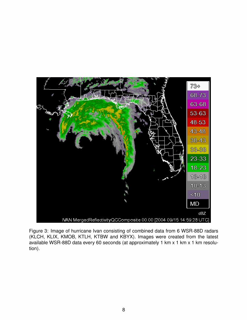
Figure 3: Image of hurricane Ivan consisting of combined data from 6 WSR-88D radars(KLCH, KLIX, KMOB, KTLH, KTBW and KBYX). Images were created from the latestavailable WSR-88D data every 60 seconds (at approximately 1 km x 1 km x 1 km resolu-tion).

8

scanning strategies (Brotzge et al. 2005).When an agent is created, it extracts some information from the underlying radial: (a)

its coordinates in the radar-centric spherical coordinate system (range, azimuth, elevationangle) (b) the radial start time (c) the radar the observation came from. All these aretypically readily available in the radar data regardless of the type of radar or the presenceor absence of “volume coverage patterns.” The agent’s coordinates in the earth-centriclatitude-longitude-height coordinate system of the resulting 3D grid have to be computed,however. The agents obtain these values following the 4/3 effective earth radius modelof Doviak and Zrnic (1993) (assuming standard beam propagation).

For a grid point in the resulting 3D grid (“voxel”) at latitude αg, longitude βg and at aheight hg above mean-sea-level, the range gate that fills it, under standard atmosphericconditions, is the range gate that is a distance r from the radar (located at (αr,βr,hr) in3D space) on a radial at an angle a from due-north and on a scan tilted e to the earth’ssurface where a is given by:

a = sin−1(sin(π/2− αg) sin(βg − βr)/ sin(s/R)) (1)

where R is the radius of the earth and s is the great-circle distance, given by (Beyer 1987):

s = R cos−1(cos(π/2− αr) cos(π/2− αg)+

sin(π/2− αr) sin(π/2− αg) cos(βg − βr))(2)

the elevation angle e is given by (Doviak and Zrnic 1993):

e = tan−1cos(s/IR)− IR

IR+hg−hr

sin(s/IR)(3)

where I is the index of refraction, which under the same standard atmospheric conditionsmay be assumed to be 4/3 (Doviak and Zrnic 1993), and the range r is given by:

r = sin(s/IR)(IR + hg − hr)/ cos(e) (4)

Since the sin−1 function has a range of [−π, π], the azimuth, a, is mapped to the correctquadrant ([0, 2π]) by considering the signs of αg − αr and βg − βr. The voxel at αg, βg, hg

can be affected by any range gate that includes (a,r,e).An agent’s life cycle depends on the radar scan. If the radar does not change its

volume coverage pattern (VCP), an agent can expect to be replaced Ttot + Ti + Tlat later,where Ttot is the expected length of the volume scan, Ti the time taken to collect the scanthat the agent belongs to and Tlat the latency in arrival of the scan after it’s been collected.In practice, Tlat is estimated to be on the same order as Ti as otherwise, it would not bepossible to keep up with the data stream. At the end of its life cycle, the agent destroysitself. The time of the latest input radar data is used as the current time. If the radarvolume coverage pattern changes, there will be redundant agents if the periodicity of theVCPs decreases (since the older agents will be around a tad longer). On the other hand,if the periodicity lengthens, there will be a short interval of time with no agents. BecauseVCPs are set up such that periodicity decreases with the onset of weather and lengthenswhen weather moves away, there is no problem as long as the technique can reliably dealwith redundant agents from the same radar. Redundant agents from the same radar can

9

be dealt with using a time-weighting mechanism. By explicitly building in an allowance forredundant agents, radars with non-standard scanning strategies such as a phased arrayradar can oversample certain regions temporally and sense other regions less often.

Whenever an output 3D grid is desired, all the existing agents collaborate to create the3D grid. Since heterogeneous radar networks are typically not synchronized, the agentswill have to account for time differences. Naively combining all the data at a particulargrid location in the latitude-longitude-height space will lead to older data from one radarbeing combined with newer data from another radar. This will lead to problems in theinitiation and decay phases of storms resulting in severe problems in the case of fast-moving storms. The agents, therefore, move to where they expect to be at the time of thegrid. For example, an agent corresponding to a radar scan t seconds ago would move tox1, y1 where:

x1 = x + uxy ∗ ty1 = y + vxy ∗ t

(5)

where x, y are the coordinates obtained from the raw azimuth-range-elevation values anduxy, vxy are horizontal motion vectors at x, y (scaled to the units of the grid). Becauseof the difficulty of obtaining a vertical motion estimate, the vertical motion is assumed tobe zero. The motion estimate may be obtained either from a numerical model or from aradar-based tracking technique such as Lakshmanan et al. (2003b). We use the latter inthe results reported in this paper.

b. Virtual Volume

Whenever a new elevation scan is received from any of the radars contributing to the3D grid, a set of agents is created. The elevation scan radial data are scale-filtered tofit the resolution of the target 3D grid. For example, if the radial data are at 0.25 kmresolution but the 3D grid is at a 1 km resolution, a moving average of four gates is usedto yield the effective elevation scan at the desired scale. Instead of creating an agentcorresponding to each range gate with valid values, we invert the problem and create anagent for each voxel in the 3D latitude-longitude-height grid that each such range gateimpacts. The influence of a range gate from the center of the range gate extends to halfthe beamwidth in the azimuthal direction and half the gate width in the range direction.This is a nearest-neighbor analysis in the azimuth and range directions. In the elevationdirection, the influence of this observation is given by δe where

δe = exp(α3ln(0.005))α = e−θi

|θi±1−θi|∨bi

(6)

α is the angular separation of the voxel from the center of the beam of an elevation scan(at elevation e) as a fraction either of the angular distance to the next higher or lower beamor the beamwidth. The ∨ is a maximum operation, bi the beamwidth of the elevation scanand θi the elevation angle of its center. This function, shown in Figure 4, is motivatedby the fact that it is 1 at the center of the beam, goes to 0.5 at half-beamwidth and fallsto below 0.01 at the beamwidth (beyond which the influence of the range gate can bedisregarded). It can be seen that where the elevation weight δe is less than 0.5, the voxelis outside the effective beamwidth of the radial. Points within the effective beamwidth are

10

Figure 4: Weighting function for interpolation between the centers of radar beams. α isthe fraction of the distance to the next higher or lower beam.

11

Figure 5: Interpolation in the spherical coordinate system mitigates bright-band effects inthis stratiform event. The data are from KDYX, KFDR, KLBB, KMAF and KSJT on 06 Feb.2005.

weighted more than they would be in a linear weighting scheme. The direction of theweighting is neither vertical nor horizontal, but tangential to the direction of the beam.

It should be noted that this interpolation is in the spherical coordinate system, in adirection orthogonal to the range-azimuth plane. Zhang et al. (2005) interpolate either inthe vertical or in both the vertical and horizontal directions (i.e. in the coordinate system ofthe resulting 3D grid). Our technique is more efficient computationally, but could fail in thepresence of strong vertical gradients such as bright bands, stratiform rain or convectiveanvils. Figure 5 demonstrates one case where spherical coordinate interpolation maysuffice, but closer examination of a larger number of cases is needed. The optimal methodfor interpolation might be neither the spherical interpolation nor the vertical-horizontalinterpolation, but to interpolate in a direction normal to the gradient direction (in 3D space).

12

3. Combining radar data

The methodology of performing objective analysis on radar reflectivity data is relativelyclear. In Section 2, we introduced a formulation of interpolating radar data on to a uniformgrid that can address problems that arise in being able to perform the required computa-tions in real-time. In this section, we describe the application of the formulation describedabove to combining radar reflectivity, radial velocity and derived products.

a. Combining scalar Data

All the intelligent agents that impact a particular voxel need to collaborate to determinethe value at that voxel. In the case of scalar data, if each intelligent agent is aware ofits influence weight, this reduces to determining a weighted average. The agent candetermine its weight simply as an exponentially declining function of its distance from theradar. However, there could be multiple agents from the same radar that affect a voxel.In the case of a radar like TDWR, there could be multiple scans at the same elevationangle within a volume scan. In the case of voxels that do not lie within a beamwidth, theremay be two agents corresponding to the adjacent elevation scans that straddle this voxel.Also, decaying or slowly moving storms often pile up agents into the same voxel due tothe resolution of the grid points. Using all these observations together, regardless of thereason there are multiple agents from the same radar, should lead to a statistically morevalid estimate.

There are two broad strategies to resolve this problem of having multiple observations(agents) from the same radar. One strategy is to devise a best estimate from each radarand then combine these estimates into an estimate for all the radars. The other is tocombine all the agents regardless of the radar they come from. In the case of velocitydata, we use the former technique while in the case of scalar data, the source of the datais ignored. However, to mitigate the problem of multiple, repeated elevation scans, thedata are weighted both by time and distance. The influence weight of an observation isgiven by:

δ = δe ∗ exp(−(t2r2/β)) (7)

where: δe is the elevation angle weight (See Eq. 6); t is the time difference between thetime the agent was created (when the radar observation was made) and the time of thegrid; r is the range of the range gate from which this observation was extracted; β is aconstant of 17.36 sec2 km2, a number that was chosen through experimentation. Amonga range of factors that we tried, this value seemed to provide the smoothest transitionswhile retaining much of the resolution of the original data.

The weighted sum of all the observations that impact a voxel is then assigned to thatvoxel in the 3D grid. This grid is used for subsequent severe weather product computa-tions.

b. Combining velocity data

Unlike the methodology of combining scalar data, the methodology of combining velocitydata in real-time is not clear. Traditional multi-Doppler wind field retrieval is computa-tionally intractable, because of its reliance on numerical convergence. In this paper, wepresent three potential solutions to this problem: (a) of computing an “inverse” Velocity

13

Azimuth Display (VAD) (b) of performing a multi-Doppler analysis, with certain approxi-mations in order to keep it tractable (c) of forgoing the wind-field retrieval altogether, butmerging shear, a scalar field derived from the velocity data. All three of the above tech-niques are applied after dealiasing the velocity data. For both the WSR-88D and TDWRdata, we apply the operational WSR-88D dealiasing algorithm. The intelligent agents forcombining velocity data are created in the same manner as in the case of combiningscalar data, but their collaborative technique is not an objective analysis one.

The multi-Doppler technique is based on the over-determined dual-Doppler techniqueof Kessinger et al. (1987). The terminal velocity was estimated from the equivalent radarreflectivity factor (Foote and duToit 1969). We initially attempted a full 3D version of themulti-Doppler technique, because severe storms do contain regions of strong vertical mo-tion, and it would be advantageous to estimate the full 3D wind field. Unfortunately, testresults for the full 3D technique were unsatisfactory. The vertical velocities in that tech-nique, computed via the mass continuity equation, turned out to be numerically unstableand propagated errors into the horizontal wind fields. Instead of abandoning the pro-cess entirely, we decided to try a simplified version of the technique, which assumes thatw = 0. Despite the fact that this assumption of w = 0 will not be valid for some regions ofsevere storms, initial test results for this 2D version of the technique were promising (Wittet al. 2005). Test results for the 2D version of the technique on two severe weather casesshowed very good agreement between the calculated horizontal wind field and corre-sponding radial velocity data. The 2D wind field also closely matched what conceptualmodels of the air flow in severe storms would suggest.

An example of merging reflectivity and velocity data from two heterogeneous radars –KTLX, a WSR-88D, and OKC, the Oklahoma City TDWR – is shown in Figure 6. A singlehorizontal level, at 1.5 km above mean sea level, is shown for the merged products. Itshould be noted that the reflectivity images from the two radars, KTLX and OKC, aredifferent because the KTLX scan is 5 minutes older than the OKC one and the stormhas moved in the time interval. The merged radar grid does have the storm in the rightlocation at the reference time. Note also that the wind field retrieval has correctly identifiedthe rotation signature.

Since the vertical motion computed from an over-determined dual-Doppler techniqueis not useful, we sought to examine if a more direct way of computing 2D horizontal windfields from the radar data was feasible. The Velocity Azimuth Display (VAD) techniquemay be used to estimate the U and V wind components from the radial velocity observa-tions using a discrete Fourier transform (Lhermitte and Atlas 1961; Browning and Wexler1968; Rabin and Zrnic 1980). The VAD technique uses a least squares approximationto calculate the first harmonic from the radial velocity observations at different azimuthsas observed from the radar location. The ”inverse” VAD technique similarly uses a leastsquares solution to determine the 2D wind components at a point in space from the radialvelocity observations from different azimuths (i.e. as observed from different radars).

The radial velocity observed from the ith radar, vi, is dependent on the wind compo-nents uo, vo and the observing angles φi of the radars:

Vn×1 = Pn×2[uovo]T (8)

where:Vn×1 = [v1v2v3...vn]T (9)

14

a b

c d

e

Figure 6: A multi-Doppler wind field retrieval is shown superimposed on data from twocomponent radars – KTLX which is a WSR-88D and OKC which is a TDWR. (a) Reflec-tivity from OKC on 08 May, 2003 at 22:35 UTC (b) Velocity from OKC (c) Reflectivity fromKTLX. The data from KTLX is from a time 4 minutes earlier than that of the OKC radar.(d) Velocity from KTLX (e) Merged reflectivity and wind field at 1.5 km above mean sealevel. The range rings from the radars are 5 km apart.

15

and Pn×2 is given by: sinφ1 cosφ1

sinφ2 cosφ2

...sinφn cosφn

(10)

If one has the radial velocity observations and the azimuth of the observations, a leastsquares approximation of the wind components may be estimated using a least-squaresformulation as:

[uovo]T = (P T

n×2Pn×2)−1(P T

n×2Vn×1) (11)The inverse VAD technique is viable as long as there are some radial velocity obser-

vations from nearly orthogonal angles.In Figure 7, we demonstrate the technique on a simulation of three CASA radars. The

radial velocity data were created from a network of simulated radars observing the numer-ical simulation (Biggerstaff and May 2005) of a tornadic storm. The inverse-VAD wind fieldtechnique was used to retrieve the 2D wind field from the Doppler velocity correspondingto the three simulated radars. The circulation signature is clearly identifiable in the windvector plot and correlates with the location of the shear signature in the radial velocitydata.

While it is useful to be able to perform multi-Doppler velocity analysis or inverse-VADanalysis in real-time to retrieve wind fields, the applicability of such a processing is limitedto radars that are somewhat proximate to each other, and situated such that the radars’viewing angles are nearly orthogonal to each other.

If we were to consider the WSR-88D network alone, such situations are rare andmade more so by the fact that unlike reflectivity data where the surveillance scans go outto 460 km, velocity data go out only to about 230 km. Thus, there are few places wheresuch analysis may be performed. In this paper, we suggested the use of TDWR radarsin addition to the WSR-88D network to increase areas of overlap and showed that theresults were promising, at least for horizontal wind vectors. However, the combinationof data from radars of different wavelengths requires further study. We demonstratedthe merging of data from a S-band radar and a C-band radar in this paper, but in thatparticular instance, there was no noticeable attenuation in the C-band data. Besides,even in the presence of attenuation in reflectivity, velocity data might still be usable. AsCASA radars (where there will be considerable overlap between the radars in the network)are deployed more widely, the real-time multi-Doppler analysis methods described herewill become more practical.

Because of the limitations of merging velocity data to retrieve wind fields, many re-searchers, Liou (2002) for example, have examined the use of single-Doppler velocityretrieval methods. It is possible that a merger of single-radar retrieved wind fields mayprove beneficial. It is also likely that applying single-Doppler velocity retrieval methods todata from a spatially distributed set of radars might yield robust estimates of wind fields.We have limited ourselves, in this paper, to describing multi-radar retrievals of wind fieldsthat can be performed in real-time using well-understood techniques.

Traditional methods of calculating vorticity and divergence from Doppler radial velocitydata can yield unreliable results. We use a two-dimensional, local, linear least squares(LLSD) method to minimize the large variances in rotational and divergent shear cal-culations (Smith and Elmore 2004). Besides creating greater confidence in the value

16

a b

c d

e f

Figure 7: An inverse-VAD wind field retrieval is shown superimposed on data from thecomponent radars. Top to bottom, reflectivity and velocity from a simulated CASA radareast, west and north of the area of interest. The range rings are at 5 km intervals. Notethat the windfield retrieved using the inverse VAD technique has captured the thunder-storm’s rotation.

17

of intensity of meteorological features that are sampled, the LLSD method for calculatingshear values has several other advantages. The LLSD removes many of the radar depen-dencies involved in the detection of rotation and radial divergence (or radial convergence)signatures. Thus, the azimuthal shear that results from the LLSD is a scalar quantity thatcan be combined using the same technique as used for radar reflectivity as shown inFigure 8.

c. Derived Products

In addition to merging reflectivity and velocity data from individual radars into a multi-radargrid, it is possible to apply the same method of merging reflectivity data to any scalar fieldderived from the radar moment data. When doing so, it is essential to justify the reasonfor combining derived products instead of deriving the product from the combination ofmoment data since the latter is more efficient computationally.

Shear is a scalar quantity that needs to be computed in a radar-centric coordinatesystem, since it is computed on Doppler velocity data taking the direction of the radialbeam into account. Therefore, it is necessary to compute the shear on data from individ-ual radars and then combine them. Having computed the shear, we can accumulate theshear values at a certain range-gate over a time interval (typically 2-6 hours), and thenmerge the maximum value over that time period from individual radars. The strategy ofblending such a maximum value from multiple radars is to take the value whose magni-tude (disregarding the sign) is maximum. Such a ”rotation track field” (shown in Figure 9)is useful for conducting after-storm damage surveys.

Once a 3D merged grid of radar reflectivity is obtained, it is possible to run many se-vere weather algorithms on this grid. For example, a multi-radar vertical composite prod-uct is shown in Figure 3. The Vertical Integrated Liquid (VIL) was introduced in Greeneand Clark (1972) using data from a single radar. A multi-radar VIL product is shown inFigure 10. VIL estimated from storm cells identified from multiple radars is a more ro-bust estimate than VIL estimated using just one radar (Stumpf et al. 2004). Figure 11demonstrates that the multi-radar VIL is more long-lived and more robust.

Three-dimensional grids of reflectivity are created at constant altitudes above meansea level. By integrating numerical model data, it is possible to obtain an estimate ofisotherm heights. Thus, it is possible to compute the reflectivity value from multiple radarsand interpolate it to points not on a constant altitude plane, but on a constant temperaturelevel. This information, updated every 60 seconds in real-time, is valuable for forecastinghail and lightning (Stumpf et al. 2005). The inputs for a lightning forecasting applicationthat makes use of this data are shown in Figure 12).

The technique to map reflectivity levels to constant temperature altitudes is used totransform the technique of the Hail Detection Algorithm (HDA; Witt et al. (1998)) froma cell-based technique to a gridded field. A quantity known as the Severe Hail Index(SHI) vertically integrates reflectivity data with height in a fashion similar to VIL. However,the integration is weighted based on the altitudes of several temperature levels. In acell-based technique, this is done using the maximum dBZ values for the 2D cell featuredetected at each elevation scan. For a grid-based technique, the dBZ values at eachvertical level in the 3D grid are used, and compared to the constant temperature altitudes.From SHI we compute Probability of Severe Hail (POSH) and Maximum Expected Hail

18

a b

c d

Figure 8: (a) Vertical slice through azimuth shear computed from a volume of data fromthe KLBB radar on 03 May 2003. (b) Azimuthal shear computed from a single elevationscan. (c) Vertical slice through multi-radar merged azimuthal shear from KFDR, KAMA,KLBB and KFWS. (d) 6 km horizontal slice through multi-radar data.

19

Figure 9: A rotation track field created by merging the maximum observed shear overtime from single radars. The overlaid thin lines indicate the paths observed in a post-event damage survey. Note that the computed path of high shear corresponds nicely withthe damage observed. Data from 03 May 1999 in the Oklahoma City area are shown.

20

Figure 10: Multi-radar Vertical Integrated Liquid product at a high-resolution spatial (ap-proximately 1 km x 1 km) and temporal (60 second update) resolution from the latestreflectivity data from four radars – KFDR, KAMA, KLBB and KFWS on 03 May 2003.

Size (MEHS) values, also plotted on a grid (See Figure 2). Having hail size estimates ona geospatial grid allows warning forecasters to understand precisely where the largest hailis falling. These grids can also be compared across a time interval to map the swathesof the largest hail or estimate the hail damage by combining hail size and duration of hailfall. These hail swathes can later be used to enhance warning verification. They can alsobe used to provide 2D aerial locations of hail damage to first responders in emergencymanagement and in the insurance industry.

3D reflectivity grids can also used to identify and track severe storm cells, and to trendtheir attributes. This is presently done using two techniques. The first is a method similarto that developed for the Storm Cell Identification and Tracking (SCIT) algorithm, that usesa simple clustering method to extract cells of a given area and vertical extent (Johnsonet al. 1998). Another technique is to compute the motion estimate directly from derivedproducts on the 3D grid following Lakshmanan et al. (2003b). For example, either themulti-radar VIL or the multi-radar reflectivity vertical composite may be used as the inputframes to the motion estimation technique. A K-Means clustering technique is used toidentify components in these fields.

Once the storms have been identified from the images, these storms are used as atemplate and the movement that minimizes the absolute-error between two frames is com-puted. Typically, frames 10 or 15 minutes apart are chosen. Given the motion estimatesfor each of the regions in the image, the motion estimate at each pixel is determinedthrough interpolation. This motion estimate is for the pair of frames that were used inthe comparison. We do temporal smoothing of these estimates by running a Kalmanfilter (Kalman 1960) at each pixel of the motion estimate. The Kalman estimator is builtaround a constant acceleration model with the standard Kalman update equations (Brownand Hwang 1997). This motion estimation technique is used as a source of uxy, vxy, the

21

Figure 11: VIL computed on cells detected from data blended from individual radars ismore robust than VIL computed on storms cells identified from a single radar. As thestorm approaches the radar, the single radar VIL drops since higher elevation data areunavailable. The multi-radar product does not have that problem. Image courtesy Stumpfet al. (2004).

22

a b

c d

Figure 12: (a) Current lightning density. (b) Reflectivity at height of -100C temperature,used as input to the lightning prediction. (c) 30-minute lightning forecast. (d) Actuallightning 30 minutes later.

23

anticipated movement of the intelligent agent currently at x, y in the 3D grid (see Eq. 5).

4. Extensions to Method

While the basic technique of creating intelligent agents and combining them yields rea-sonable results, we extended the basic technique by correcting for beam blockage fromindividual radars, improving the quality of the input data, correcting for time differencesbetween the radars, and devising optimizations to enable the technique to be used inreal-time.

a. Corrections for Beam Blockage

A range gate from a radar elevation scan is assumed to not impact a voxel if it falls withina beam-blockage umbrella due to terrain. Currently, for reasons that will become evidentin Section 4c, a standard atmospheric model with an effective 4/3 earth radius (Doviakand Zrnic 1993) is assumed to determine which radar beams will be blocked by terrainfeatures. A terrain Digital Elevation Map (DEM) at the scale of the desired grid (approx-imately 1km × 1km) was used for the results presented here, but the technique wouldapply even if higher resolution terrain maps were used.

The assumptions for a beam being blocked follow very closely the technique of O’Bannon(1997); Fulton et al. (1998). Interested readers should consult those papers for further in-formation. For each point in the DEM, the azimuth, range and elevation angle of a thinradar beam is computed following the standard beam-propagation assumptions and tol-erances as given by O’Bannon (1997). Any thin beam above this elevation angle passesabove this terrain point unblocked. Other beams are assumed to be blocked by this el-evation point. Every radial from the radar is then considered a numerical integrand ofall the thin beams that fall within its range of azimuths and elevations. The influence ofthe individual thin beams follows the power density function of Doviak and Zrnic (1993).Thus, a fraction of the beam that is blocked is known at each range gate. If this fractionis greater than 0.5, the entire range gate is assumed to be blocked – the data from suchrange gates are not used to create new intelligent agents. However, due to advection, it ispossible that a voxel that would be beam blocked might get a value due to the movementof an agent created from a non-blocked range gate. Beam-blocked voxels can also getfilled in by data from other, nearby radars, leading to a more uniform spatial coveragethan what is possible using just one radar. Figure 13 demonstrates the filling of data fromadjacent radars to yield better spatial coverage when some parts of a radar domain arebeam-blocked.

Similar to the beam blockage correction, it should be possible to dynamically correctfor inaccurate clocks on individual radars and for heavy attenuation from individual radars.Our current implementation does neither because of our initial focus on the WSR-88Dnetwork. The inaccurate clocks on the WSR-88D network are to be fixed with automatictime-correction software in the radar sites. WSR-88Ds, being S-band radars, do not at-tenuate as severely as X-band radars. For C-band radars such as TDWR and X-bandradars such as those that will be used in the CASA network, an attenuation correction willhave to be put in place to avoid an under-reporting bias in the multiple radar grids.

24

a b

c d

Figure 13: (a) Vertical slice through data from the KIWA (Phoenix) radar on 14 Aug. 2004.(b) Elevation scan from the KIWA radar. Note the extensive beam blockage. (c) Verticalslice through multi-radar data from KIWA, KEMX, KYUX, KFSX and KABX covering thesame domain. (d) 5 km horizontal slice through multi-radar data. Note that the entiredomain is filled in.

25

b. Quality Control of Input Data

Weather radar data are subject to many contaminants, mainly due to non-precipitatingtargets (such as insects and wind-borne particles) and due to anomalous propagation(AP) or ground clutter. If the radar data are directly placed into the 3D merged grid, theseartifacts lower the quality of the gridded data. Hence, the radar velocity data need tobe dealiased and the radar reflectivity data need to be quality controlled. We used thestandard WSR-88D dealiasing algorithm to dealias the velocity data.

In radar reflectivity data, several local texture features and image processing stepscan be used to discriminate some types of contaminants (Kessinger et al. 2003). How-ever, none of these features by themselves can discriminate between precipitating andnon-precipitating areas. A neural network is used to combine these features into a dis-crimination function (Lakshmanan et al. 2003a). Figure 14 demonstrates that the neuralnetwork is able to identify, and remove, echoes due to anamalous propagation while re-taining echoes due to precipitation.

No current technique using only single radar data (ignoring polarimetric data) candiscriminate between shallow precipitation and spatially smooth clear-air return (Laksh-manan and Valente 2004). The radar-only techniques also have problems removing somebiological targets, chaff and terrain-induced ground clutter far away from the radar. In ad-dition to the radar-only quality control above, an additional stage of multi-sensor qualitycontrol is applied. This uses satellite data and surface temperature data to remove clear-air echoes. Figure 15 demonstrates that biological returns may be removed by usingsuch cloud cover information. For more details, the reader is directed to Lakshmanan andValente (2004).

The radar reflectivity elevation scans are quality controlled, either using the radar-only quality-control technique described in Lakshmanan et al. (2003a) or using the multi-sensor technique described in Lakshmanan and Valente (2004). It is these quality-controlledreflectivity data that are presented to the agent framework for incorporation into the con-stantly updating grid.

c. Precomputation

The coordinate system transformation to go from each voxel αg, βg, hg to the sphericalcoordinate system (a,r,e) can be precomputed as long as we limit the input radars to benonmobile units (so that the radar position does not change). If the radar follows one ofa set number of volume coverage patterns, then the elevation scan can be determinedfrom e. If the elevation scans are indexed to always start at a specific azimuth and eachbeam constrained to an exact beam width (WSR-88D scans are not), then a, r can alsobe mapped to specific locations in the radar array. In fact, the presence of a volume cov-erage pattern is not required to precompute the effect of data from an elevation angle –all that’s required is that the radar operate only at a limited number of elevation angles,perhaps in a range of [0o, 20o] in increments of 0.1o. Then, the voxels impacted by datafrom an elevation scan can be computed beforehand and stored in permanent memory(hard drive) for immediate recall whenever that elevation angle from that radar is received.Intelligent agents can be then created, assigning to them the coordinates in both coordi-nate systems at the time of creation. If the VCPs are known or if the radar operates onlyat set elevations, it is possible to precompute the elevation weight δe. However, because

26

a b

c d

Figure 14: Independent test cases for the Quality Control Neural Network (QCNN): (a) Adata case from KAMA with significant AP. The range rings are 50 km apart. (b) Editedusing the neural network – note that all the AP has been removed, but the storm cellsnorth west of the radar are retained. (c) Typical spring precipitation (d) Edited using theneural network – note that even the storm cell almost directly overhead the radar hasbeen retained, but biological scatter has been removed.

27

a b

c d

Figure 15: (a) Radar (KTLX) reflectivity composite showing effects of biological contami-nation. (b) The cloud-cover field derived from satellite data and surface observations. (c)The effect of the radar-only quality control neural network. (d) The effect of using boththe radar-only neural network and the cloud cover field. Note that the small cells to thenorth-west of the radar are unaffected, but the biological targets to the south of the radarare removed.

28

of the dependence on t, a time-delay variable, it is necessary to compute δ at the time ofgrid creation. Similarly, the presence of t in the advection equations necessitates that themovement of the agents to their new positions be dynamic and not precomputed.

These precomputations have to be performed for every possible elevation angle fromevery radar that will be used as an input to the merged 3D grid. For a grid of approximately800km × 800km and about 10 radars, a typical regional domain, the precomputation cantake up to 8 hours on a workstation with a 1.8GHz Intel Xeon processor, 2GB of randomaccess memory and a 512 MB cache (referred here on as simply Intel Xeon). Thus, it isnecessary to decide upon a regional domain well in advance of the storm event, or haveenough hardware available to process a large radar domain reflecting the threat 6-8 hoursin advance.

d. Extraction of subdomains

Naturally, determining the domain of interest 6-8 hours in advance is not a trivial task. Is itpossible to reuse precomputations? Because the coordinate system of the output 3D gridis a rectilinear system (the αg, βg, hg are additive), we can precompute the transformationof data from any radar in the country at every elevation angle possible onto a domainthe size of the entire continental United States (CONUS). The CONUS domain can becreated at the desired resolution. We currently use 0.01 degrees in latitude and longitudeand 1km in height, approximately 1km × 1km × 1km at mid-latitudes. Then, the coordi-nates of the range gate in a subdomain of the CONUS domain can be computed fromits coordinates in the CONUS domain using the offsets of the corners. If the north-westcorner of the CONUS domain is αc, βc, hc and that of the desired subdomain is αs, βs, hs,then the additive correction to the αg, βg, hg entries in the CONUS cache to yield correctsubdomain entries is:

δα = (αg − αc)/resα

δβ = (βc − βg)/resβ(12)

where resα, resβ are the resolution of the 3D grid in the latitudinal and longitudinal direc-tions. The only condition is that the above operations have to yield integers, since they willbe indexes into the CONUS domain arrays. Thus, the limitation is that subdomains haveto be defined at 0.01 degree/1 km increments. Computation of the CONUS domain takesabout 120 hours on a dual-processor workstation and requires 77GB of disk space. How-ever, this needs to be done only once and can be farmed out to a bank of such machinesto cut down the computation time. With this precomputed CONUS domain, we gain theability to quickly switch domains. See Levit et al. (2004) for how this capability is used toget real-time access to merged 3D radar data from anywhere in the country using a singleworkstation.

e. Time Correction

Motion estimates obtained from the technique described in Lakshmanan et al. (2003b) areused to correct for time differences between the sensing of the same storms by differentradars using Eq. 5. This dramatically improves the value of derived products computedfrom the 3D grid because, by correcting the locations of the storms, the areas sensed bydifferent radars line up in space and time. Figure 2 demonstrates the significant differencebetween an uncorrected image and a time-corrected one.

29

The characteristics of the motion estimation technique impact the results in the mergedgrid. If motion of a few storms is underestimated, then those storms will appear to jumpwhenever newer data are obtained, as the intelligent agents correct their positions. Sincethe motion estimation technique of Lakshmanan et al. (2003b) is biased toward estimatingthe movement of larger storms correctly, smaller cells and cells with erratic movementswill tend to not provide smooth transitions. However, the transition in such cases willtypically still be less than the transition that would have resulted if no advection correctionhad been applied.

Weighting individual observations by time (in addition to distance; see Eq. 7) can haveundesirable side effects if the radars are not calibrated identically. If one radar is “hotter”than all the others, then in those time frames where data from that radar is the latest avail-able, the merged image will appear hotter. This problem affects radar data from the WSR-88D network because of large calibration differences between individual radars (Gourleyet al. 2003) and is most evident when viewing time sequences of merged radar data.

In the absence of time weighting, however, the merged data will be a biased estimatein areas where the storms are exhibiting fast variations in intensity because older data arestill retained. The older data are advected to their correct positions, but no compensationis made for potential changes in intensity since automated extraction of the growth/decayof the storm was found to possess very little skill (Lakshmanan et al. 2003b). There-fore, calibration differences still remain evident when looking at features that migrate fromthe domain of one radar to the domain of another, especially when these features areaccumulated over time.

One solution to the problem when combining time weighting with calibration differ-ences between radars is to retain time weighting but to apply calibration corrections to thedata from individual radars. We intend to implement such a calibration correction in futureresearch.

f. Timing

The time taken to read individual elevation scans, update the 3D grid by creating intelli-gent agents and write the current state of the 3D grid periodically depends on a varietyof factors. We carried out a test where the individual elevation scans and the output gridare both compressed (as will be the case in a networked environment, to conserve band-width), so all these timing data reflect the time taken to uncompress while reading andcompress when writing. We carried out this test for a 650× 700× 18 regional domain withconvective activity in most parts of the region and using data from 3 WSR-88Ds. Differenttasks scale to either the domain size or the number of radars. These are marked alongwith the timing information in Table 1. The test was carried out on the aforementionedIntel Xeon workstation.

Table 1 can be used to determine the computing power needed for different domainsizes and numbers of radars. On average, we require 0.5 seconds per elevation scanand 2.75 seconds per million voxels. It should be noted that merging radar data using thetechnique described in this paper is an “embarrassingly parallel” problem i.e., if multiplemachines are put to work on the problem, each machine can concentrate on a subdomainand the output grids can be cheaply stitched together again. The subdomains do have topartially overlap to take into account advection effects.

30

Aspect CPU Time s Clock Time s Scaling

Read radar scan 0.012 ± 0.001 0.254 ± 0.023 One elevation scan

Update grid with scan 0.075 ± 0.007 1.28 ± 0.135 One elevation scan

Create 3D grid 0.594 ± 0.127 9.179 ± 2.056 8m voxels

Write 3D grid 1.257 ± 0.268 20.68 ± 4.62 8m voxels

Table 1: Timing statistics collected in real-time for reading radar data and creating 3Dmerged grids of reflectivity.

Update interval Domain size Radars Domain resolution No. of machines

CONUS 1 minute 5000km× 3000km× 20km 130 1km× 1km× 1km 20

Regional 1 minute 800km× 800km× 20km 10 1km× 1km× 1km 1

CONUS 5 minute 5000km× 3000km× 20km 130 1km× 1km× 1km 4

Table 2: Estimated hardware requirements to implement this technique. The machinereferred to here is a 1.8 GHz Intel Xeon processor with 2 GB of RAM.

Using the information in Table 1, we can estimate the computational requirements tocreate a 5000 × 3000 × 20 domain every 60 seconds in real-time using information from130 WSR-88Ds. Let us estimate that we will receive a new elevation scan from eachof the radars every 30 seconds (in areas having significant weather, this will be around20 seconds while in areas of little weather, the interval approaches 120 seconds). Thus,we will have 260 elevation scans per minute to read and update, which will take about130 wall-clock seconds on our single workstation. Since our 5000 × 3000 × 20 domaincontains 300 million voxels, creating and writing out the grid will take 1125 more seconds.Our single workstation, if outfitted with enough computer memory, will be able to createand write 3D merger grids for this domain in 1250 seconds. To maintain our updateinterval of 60 seconds, we would require about 20 such workstations. The hardwarerequirements for several scenarios are provided in Table 2. Levit et al. (2004) used theregional configuration in their study.

5. Summary

In this paper, we described a technique based on an intelligent agent formulation for tak-ing the base radar data (reflectivity and radial velocity), and derived products, from mul-tiple radars and combining them in real-time into a rapidly updating 3D merged grid. We

31

demonstrated that the intelligent formulation accounts for the varying radar beam geom-etry with range, vertical gaps between radar scans, lack of time synchronization betweenradars, storm movement, varying beam resolutions between different types of radars,beam blockage due to terrain, differing radar calibration and inaccurate time stamps onradar data.

The techniques described in this paper of merging moment data from individual radarshave been tested in real-time, and on archived data cases, in diverse storm regimes. Theyhave been tested on different types of radars as well. For example, Figure 3 shows thetechnique operating in a hurricane event. Figure 13 shows the technique operating onlate-summer monsoon events in an area with terrain. Figures 2, 9 and 10 illustrate theuse of this technique in convective situations, while Figure 5 illustrates a stratiform one.One of the radars in Figure 6 is a TDWR while the others are WSR-88Ds, while Figure 7shows simulated CASA radars.

With the continuing improvements in computer processors, operating systems andinput/output performance, preliminary tests indicate that a 2-minute CONUS 3D mergercan be implemented using a single 3 GHz 64-bit processor with 8 GB of RAM. Thus, weplan to start utilizing this technique to merge scalar fields, both reflectivity and derivedshear products, from all the WSR-88D radars in the Continental United States. We nowhave the ability to ship the merged products in real-time to AWIPS/N-AWIPS workstationsat weather forecast offices and national centers. Since these workstations will be unableto handle the data at its highest resolution and spatial extent, we may have to subsectthe data before shipping it to operational centers. The merged products created using thetechnique described in this paper should be available for operational use by the time thispaper is in print.

We would also like to note that software implementing this technique of combining datafrom multiple radars is freely available at http://www.wdssii.org/ for research and academicuse.

32

Acknowledgments

Funding for this research was provided under NOAA-OU Cooperative Agreement NA17RJ1227,the National Science Foundation Grants ITR 0205628 and 0313747 and the National Se-vere Storms Laboratory. Part of the work was performed in collaboration with the CASANSF Engineering Research Center EEC-0313747. We thank Kiel Ortega for creatingsome of our data cases, Jian Zhang for her useful pointers at several stages of this re-search, Rodger Brown for guidance on the multi-Doppler velocity combination approachand the anonymous reviewers whose inputs have improved the clarity of our paper. Thestatements, findings, conclusions, and recommendations are those of the authors and donot necessarily reflect the views of the National Severe Storms Laboratory, the NationalScience Foundation or the U.S. Department of Commerce.

33

References

Adrianto, I., T. M. Smith, K.A.Scharfenberg, and T. Trafalis, 2005: Evaluation of variousalgorithms and display concepts for weather forecasting. 21st Int’l Conf. on Inter. Inf.Proc. Sys. (IIPS) for Meteor., Ocean., and Hydr., Amer. Meteor. Soc., San Diego, CA,CD–ROM, 5.7.

Askelson, M., J. Aubagnac, and J. Straka, 2000: An adaptation of the Barnes filter appliedto the objective analysis of radar data. Mon. Wea. Rev., 128, 3050–3082.

Beyer, W., ed., 1987: CRC Standard Math Tables. CRC Press Inc., 18th edition.

Biggerstaff, M. I. and R. M. May, 2005: A meteorological radar emulator for education andresearch. 21st Int’l Conf. on Inter. Inf. Proc. Sys. (IIPS) for Meteor., Ocean., and Hydr.,Amer. Meteor. Soc., San Diego, 5.6.

Brotzge, J., D. Westbrook, K. Brewster, K. Hondl, and M. Zink, 2005: The meteorologicalcommand and control structure of a dynamic, collaborative, automated radar network.21st Int’l Conf. on Inter. Inf. Proc. Sys. (IIPS) for Meteor., Ocean., and Hydr., Amer.Meteor. Soc., San Diego, CA, 19.15.

Brown, R. and P. Hwang, 1997: Introduction to Random Signals and Applied KalmanFiltering. John Wiley and Sons, New York.

Browning, K. and A. Wexler, 1968: The determination of kineatic properties of a wind fieldusing doppler rada. Journal of Applied Meteorology , 7, 105–113.

Burrows, M. and D. Wheeler, 1994: A block-sorting lossless data compression algo-rithm. Technical Report 124, Digital Equipment Corporation, Palo Alto, California, avail-able via http from gatekeeper.dec.com/pub/DEC/SRC/research-reports/abstracts/src-rr-124.html.

Charba, J. and F. Liang, 2005: Quality control of gridded national radar re-flectivity data. 21st Conference on Weather Analysis and Forecasting/17thConference on Numerical Weather Prediction, Washington, DC, 6A.5,http://www.nws.noaa.gov/mdl/radar/mosaic webpage.htm.

Doviak, R. and D. Zrnic, 1993: Doppler Radar and Weather Observations. AcademicPress, Inc., 2nd edition.

Droegemeier, K., K. Kelleher, T. Crum, J. Levit, S. D. Greco, L. Miller, C. Sinclair, M. Ben-ner, D. Fulker, and H. Edmon, 2002: Project CRAFT: A test bed for demonstrating thereal time acquisition and archival of WSR-88D Level II data. Preprints, 18th Int’l Conf. onInter. Inf. Proc. Sys. (IIPS) for Meteor., Ocean., and Hydr., Amer. Meteor. Soc., Orlando,Florida, 136–139.

Foote, G. and P. S. duToit, 1969: Terminal velocity of raindrops aloft. J. App. Meteor., 8,249–253.

34

Fulton, R., D. Breidenback, D. Miller, and T. O’Bannon, 1998: The WSR-88D rainfallalgorithm. Weather and Forecasting, 13, 377–395.

Gourley, J. J., B. Kaney, and R. A. Maddox, 2003: Evaluating the calibrations of radars:A software approach. 31st Int’l Conf. on Radar Meteor., Amer. Meteor. Soc., Hyannis,MA, P3C.1.

Greene, D. R. and R. A. Clark, 1972: Vertically integrated liquid water – A new analysistool. Mon. Wea. Rev., 100, 548–552.

Johnson, J., P. MacKeen, A. Witt, E. Mitchell, G. Stumpf, M. Eilts, and K. Thomas, 1998:The storm cell identification and tracking algorithm: An enhanced WSR-88D algorithm.Weather and Forecasting, 13, 263–276.

Kalman, R., 1960: A new approach to linear filtering and prediction problems. Trans.ASME – J. Basic Engr., 35–45.

Kessinger, C., S. Ellis, and J. Van Andel, 2003: The radar echo classifier: A fuzzy logicalgorithm for the WSR-88D. 19th Int’l Conf. on Inter. Inf. Proc. Sys. (IIPS) for Meteor.,Ocean., and Hydr., Amer. Meteor. Soc., Long Beach, CA.

Kessinger, C. J., P. Ray, and C. E. Hane, 1987: The Oklahoma squall line of 19 may 1977.part 1: A multiple Doppler analysis of convective and stratiform structure. J. Atmos. Sci.,44, 2840–2864.

Lakshmanan, V., K. Hondl, G. Stumpf, and T. Smith, 2003a: Quality control of weatherradar data using texture features and a neural network. 5th Int’l Conf. on Adv. in Patt.Recogn., IEEE, Kolkota.

Lakshmanan, V., R. Rabin, and V. DeBrunner, 2003b: Multiscale storm identification andforecast. J. Atm. Res., 367–380.

Lakshmanan, V. and M. Valente, 2004: Quality control of radar reflectivity data usingsatellite data and surface observations. 20th Int’l Conf. on Inter. Inf. Proc. Sys. (IIPS)for Meteor., Ocean., and Hydr., Amer. Meteor. Soc., Seattle, CD–ROM, 12.2.

Levit, J. J., V. Lakshmanan, K. L. Manross, and R. Schneider, 2004: Integration of theWarning Decision Support System - Integrated Information (WDSS-II) into the NOAAStorm Prediction Center. 22nd Conference on Severe Local Storms, Amer. Meteor.Soc., CDROM.

Lhermitte, R. and D. Atlas, 1961: Precipitation motion by pulse doppler. 9th Conferenceon Radar Meteorology , Boston, 218–223.

Liou, Y.-C., 2002: An explanation of the wind speed underestimation obtained from aleast squares type single-doppler radar velocity retrieval method. J. App. Meteor., 41,811–823.

Maes, P., 1995: Artificial life meets entertainment: Life like autonomous agents. Commu-nications of the ACM, 38, 108–114.

35

McNellis, T., S. Katz, M. Campbell, and J. Melody, 2005: Recent advances in phased arrayradar for meteorological applications. 21st Int’l Conf. on Inter. Inf. Proc. Sys. (IIPS) forMeteor., Ocean., and Hydr., Amer. Meteor. Soc., San Diego, CA, 19.6.

O’Bannon, T., 1997: Using a terrain-based hybrid scan to improve WSR-88D precipitationestimates. 28th Conf. on Radar Meteorology , Amer. Meteor. Soc., Austin, TX, 506.

Rabin, R. and D. Zrnic, 1980: Subsynoptic-scale vertical wind revealed by dual Doppler-radar and VAD analysis. J. Atmos. Sc., 37, 644–654.

Smith, D. C., A. Cypher, and J. Spohrer, 1994: KidSim: Programming agents without aprogramming language. Communications of the ACM, 37, 55–67.

Smith, T. M. and K. L. Elmore, 2004: The use of radial velocity derivatives to diagnoserotation and divergence. 11th Conf. on Aviation, Range, and Aerospace, Amer. Meteor.Soc., Hyannis, MA, CD–ROM.

Stumpf, G., S. Smith, and K. Kelleher, 2005: Collaborative activities of the NWS MDL andNSSL to improve and develop new multiple-sensor severe weather warning guidanceapplications. 21st Int’l Conf. on Inter. Inf. Proc. Sys. (IIPS) for Meteor., Ocean., andHydr., Amer. Meteor. Soc., San Diego, CA, CD–ROM, P2.13.

Stumpf, G. J., T. M. Smith, and J. Hocker, 2004: New hail diagnostic parameters derivedby integrating multiple radars and multiple sensors. 22nd Conf. on Severe Local Storms,Amer. Meteor. Soc., Hyannis, MA, P7.8.

Trapp, R. J. and C. A. Doswell, 2000: Radar data objective analysis. J. Atmos. Ocean.Tech., 17, 105–120.

Witt, A., R. A. Brown, and V. Lakshmanan, 2005: Real-time calculation of horizontal windsusing multiple doppler radars: A new WDSS-II module. 32nd Conference on RadarMeteorolog, Amer. Meteor. Soc., Albuquerque, NM.

Witt, A., M. Eilts, G. Stumpf, J. Johnson, E. Mitchell, and K. Thomas, 1998: An enhancedhail detection algorithm for the WSR-88D. Weather and Forecasting, 13, 286–303.

Zhang, J., K. Howard, and J.J.Gourley, 2005: Constructing three-dimensional multiple-radar reflectivity mosaics: Examples of convective storms and stratiform rain echoes. J.Atmos. Ocean. Tech., 22, 30–42.

36