a rebuttal to dr. hogan: "looking for the 'voom'"

8/14/2019 A Rebuttal to Dr. Hogan: "Looking for the 'Voom'"

http://slidepdf.com/reader/full/a-rebuttal-to-dr-hogan-looking-for-the-voom 1/14

Looking for the “Voom”


A Rebuttal to Dr. Hogan’s “Acting in Time: Regulating Wholesale Electricity

Markets”

Robert McCullough

June 26, 2007

In 1958, the very gifted Dr. Theodore Seuss Geisel published The Cat in the Hat Comes Back.12 While this

beloved children’s book is not normally cited as a primer for public policy, its principal character, the Cat

in the Hat, serves as a good model for the continued efforts to implement administered electricity

markets in the United States. The Cat, a charming, irresponsible individual, proposes plausible, but

increasingly disruptive, suggestions. As the story unfolds, each suggestion requires a new Cat in the Hat

to solve the resulting problems. Finally, the smallest cat of all provides a magical substance called

“Voom”

to

clear

up

the

mayhem

caused

by

the

Cat

and

his

followers.

3

Many practitioners in the electricity industry have begun to yearn for a policy “Voom” that would put

the Cat and all of his misadventures back in the hat. Dr. Hogan’s latest proposal is very much in the

tradition of Dr. Seuss’s famous protagonist. “Acting in Time: Regulating Wholesale Electricity Markets”

contains two different suggestions. The first exhorts the Federal Energy Regulatory Commission (FERC)

to continue its proactive policy in favor of replacing existing markets with centralized administered

markets. This is a basic philosophic position that represents Dr. Hogan’s belief that markets are best

implemented and administered by government. Despite the success of the Western Systems Power

Pool, formally implemented in 1991, and now in place for over twenty years, Dr. Hogan still prefers

tightly centralized structures. He is also a believer in the primacy of regulation over markets – the need

to design and administer markets for their own good. His second suggestion concerns the absence of

new resource construction.

The results of Dr. Hogan’s suggestions, like those of the Cat, have been mixed. In the mid‐1990s, he won

the debate in California to reject open markets in favor of the tightly organized and deeply administered

system that has had such a troubled history. Like the Cat, the unforeseen results were not his fault – Dr.

Hogan has frequently pointed out that it was the implementation of his ideas that was faulty. Many of

us are in substantial agreement. Whether FERC should continue its proactive stance to replace open

markets with administered markets is still the subject of debate. Some believe that having governments

design and administer markets is an oxymoron. Certainly, the increasing differential in electric rates

between those

serving

customers

in

open

market

states

and

those

serving

customers

in

administered

market states indicates that much remains to be understood about the merits of turning markets over

to centralized, quasi‐governmental agencies.

1 My thanks to the APPA for funding this research paper. All opinions and analysis are strictly my own.

2 The Cat In The Hat Comes Back, Theodore Seuss Geisel, 1958.

3 For technical details of Voom, see pages 57 through 59.




Dr. Hogan’s second suggestion is designed to solve a problem that has afflicted states being served by

administered markets – the absence of new resource construction. He notes that the “missing money”

problem is a major hindrance (the term was coined by Roy Shanker almost five years ago to describe the

absence of incentives for new generation). The crux of Dr. Hogan’s argument is that

In

particular,

prices

in

organized

markets

tend

to

be

too

low

during

conditions

of

generation capacity scarcity, exactly the time when the unexploited demand side

resource would be most valuable. But without the signal and the reward through prices,

there is insufficient market incentive for demand side action or for adequate

infrastructure investment. There are many reasons for this inadequate scarcity pricing

that relate to both mistakes in market design and practices of system operators.4

It appears, however, that Dr. Hogan does not recognize that the missing money problem is endemic to

his preference for an energy‐only administered market.

Dr. Joskow has also written on this issue in “Competitive Electricity Markets and Investment in New

Generating Capacity.”5

He

develops

a simple

electric

market

using

traditional

planning

tools,

even

going

so far as to assume values for loads and plant costs. Since technical points are always more accessible

with simple examples, I have taken the liberty of “borrowing” his example.6

Calculating the “Missing Money” in Dr. Hogan’s Paper To plan the optimal electric system, the following straightforward technique should be included in the

tool kit of every aspiring resource planner:

1. Establish the fixed and variable costs for all available resource options

2. Calculate the total cost for each resource over the 8,760 hours in the year

3. Choose the

least

cost

resource

for

each

hour

of

the

year

(the

evocative

term

economists

use

for this step is finding the “convex hull” of possible resource options)

4. Find the hour corresponding to each vertex of the convex hull

5. Determine the required capacity by reading the load off the load duration curve for that

hour.

While Dr. Joskow’s example only extends to three resource options – Base Load, Intermediate, and

Peaking, the five‐step technique works for any set of resource options as long as the costs are linear

functions of the expected dispatch. Dr. Joskow’s Table 8 assumes the following values:

Technology

Capital

Costs

($/MW/Year)

Operating

Costs

($MWh)

Base Load $240,000 $20

Intermediate $160,000 $35

4 Acting in Time: Regulating Wholesale Electricity Markets, William W. Hogan, May 8, 2007, page 5.

5 Competitive Electricity Markets and Investment in New Generating Capacity, Paul Joskow, June 12, 2006.

6 Ibid., Table 8, page 69.




Peaking $80,000 $80

The optimal mix of resources can be readily calculated by observing which plant type is best for each

level of expected operation:

The least

expensive

result

for

each

hour

is

represented

by

the

dashed

line

which

shows

the

best

choice

of resource for each level of expected operations. Not surprisingly, in this example, peakers are optimal

for operations over a small number of hours (1 through 1,777), intermediate resources dominate from

1,778 through 5,343 hours a year, and base load units are best for longer durations (5,334 hours

through 8,760 hours a year).

Prices in this very simple example are easy to derive. During high load periods, the marginal resource is

a peaker. Hence, market prices are equal to the running costs of all peakers – $80/MWh. During

shoulder hours, the marginal unit is the intermediate resource – $35/MWh. Finally, during the off ‐peak

hours, only the base load units are dispatched and the marginal cost falls to $20/MWh.

$‐

$100,000

$200,000

$300,000

$400,000

$500,000

$600,000

$700,000

$800,000

$900,000

1

2 9 3

5 8 5

8 7 7

1 1 6 9

1 4 6 1

1 7 5 3

2 0 4 5

2 3 3 7

2 6 2 9

2 9 2 1

3 2 1 3

3 5 0 5

3 7 9 7

4 0 8 9

4 3 8 1

4 6 7 3

4 9 6 5

5 2 5 7

5 5 4 9

5 8 4 1

6 1 3 3

6 4 2 5

6 7 1 7

7 0 0 9

7 3 0 1

7 5 9 3

7 8 8 5

8 1 7 7

8 4 6 9

$ / M W / Y e a r

Hours of Operation

The Optimal Convex Hull from Dr. Joskow's Example

Base Load Intermediate Peaking Minimum Cost




This makes it very easy to calculate the expected revenues for a new resource. The owner of a new

peaker would quickly note that if prices never increased above marginal cost, it would never be able to

make

any

contribution

against

its

fixed

costs.

Thus,

the

owner

would

lose

its

fixed

costs

–$80,000/MW/Year – if it invested in this market.

Surprisingly, this is also true for the owner of an intermediate resource. Although more complex, the

calculation gives the identical result. Thus, the owner’s calculation would credit the producer’s surplus

(the area above the marginal cost it would receive during peak periods) against capital costs. In this

case, the owner would receive $45/MWh ($80/MWh‐$35/MWh) for the 1,777 peak hours in the year, or

$80,000, the capital costs would be $160,000, and the net loss would be $80,000.

The owner of a base load plant fares exactly the same. The producer’s surplus is $60/MWh for the first

1,777 hours and $15/MWh ($35/MWh‐$20/MWh) for the next 5,333 hours. Overall, the producer’s

surplus

would

be

$160,000,

the

capital

costs

would

be

$240,000,

and

the

net

loss

would

be

$80,000/MWh.

$‐

$10

$20

$30

$40

$50

$60

$70

$80

$90

1

2 7 5

5 4 9

8 2 3

1 0 9 7

1 3 7 1

1 6 4 5

1 9 1 9

2 1 9 3

2 4 6 7

2 7 4 1

3 0 1 5

3 2 8 9

3 5 6 3

3 8 3 7

4 1 1 1

4 3 8 5

4 6 5 9

4 9 3 3

5 2 0 7

5 4 8 1

5 7 5 5

6 0 2 9

6 3 0 3

6 5 7 7

6 8 5 1

7 1 2 5

7 3 9 9

7 6 7 3

7 9 4 7

8 2 2 1

8 4 9 5

$ / M W h

Yearly Hours Sorted By Load

Marginal Cost




It should not be lost on the reader that this is a “Cat in the Hat” moment. As it turns out, the loss for any

new resource under any set of assumed costs and loads is always the capital cost of the resource with

the least fixed costs.7

Dr. Hogan’s solution to the missing money problem would require the regulator to add enough revenues

into the

market

to

make

new

entry

attractive.

This

is

not

an

implausible

suggestion,

although

I observe

that FERC’s competitive agenda has been neatly hijacked back to the full revenue requirements model

that Dr. Hogan’s solution expected to replace. To fix the problem, any determined market administrator

can intervene in one of four ways:

1. The market administrator could abandon the attempt to force the market into the “energy only”

model. This would entail returning to an open market solution like the WSPP. In this case,

market participants could make transactions directly with each other – pricing energy and

capacity as they saw fit.

2. The market administrator could simply add to prices by placing a tax on each megawatt‐hour

sufficient

to

reimburse

resource

developers

for

their

capital

costs.

While

this

returns

the

regulator to calculating used and useful resource costs, it is likely to be less disruptive than some

of the other options.

3. The market administrator could unilaterally move the supply curve back towards the origin by

not counting the bids of some of the base load resources. Again, this would raise the price, but

it would add some complexity.

4. Finally, the least attractive solution, the market administrator could move the demand curve

right – away from the origin – in order to raise prices. This solution is likely to move the market

away

from

optimality,

increase

volatility,

and

encourage

market

manipulation.

The following figure illustrates options 2, 3, and 4.

7 The appendix illustrates the proof with a graphical example.




Dr. Hogan has chosen the fourth solution – the addition of demand. He says:

This example of operating reserve demand curve based on representative data

illustrates several important points regarding the shape, magnitude and costs. The

shape has a simple explanation. As discussed above, there are two underlying demand

curves. One is the vertical demand curve from the security minimum defined by the

contingency constraint. Second is the more conventional demand curve defined by

probabilistic analysis and the value of expected unserved energy. The usual rules apply

to yield horizontal addition. Another way of thinking about this is that at the minimum

security level of 500 MW, the probability that net demand will exceed expected net

demand in

the

next

half

hour

is

less

than

one.

Hence,

the

curved

portion

of

the

demand

curve connects at a price below the VOLL.8





Although “Acting in Time: Regulating Wholesale Electricity Markets” does not describe what Dr. Hogan’s

revised demand curve will look like with the operating reserves addition, the eleventh slide from his

March 3, 2006 presentation offers some additional details9:

To fit Dr. Hogan’s concept into our numerical example, we must estimate the size of his assumed

reserve and how often the demand curve would intersect operating reserves.

Fortunately, sample values fall directly out of the example. If Dr. Hogan requires $80,000 to “fix” the

revenue shortfall, he will only need to add a small amount to the marginal cost curve. If the producer’s

surplus needs to be $80,000, he can achieve the result with only $80,000/($10,000‐$80), or just over 8

hours.

This result should cause some discomfort for three reasons:

1. In our simple example, tinkering with the demand curve has moved us off the optimal resource

plan. The difference is not large, but it will now mean that the market will build peakers to meet

1,785 hours (1,777 plus 8) where the marginal cost of operation is larger than or equal to spot

prices.

9 Reliability and Scarcity Pricing: Operating Reserve Demand Curves, William Hogan, March 3, 2006, slide 11.




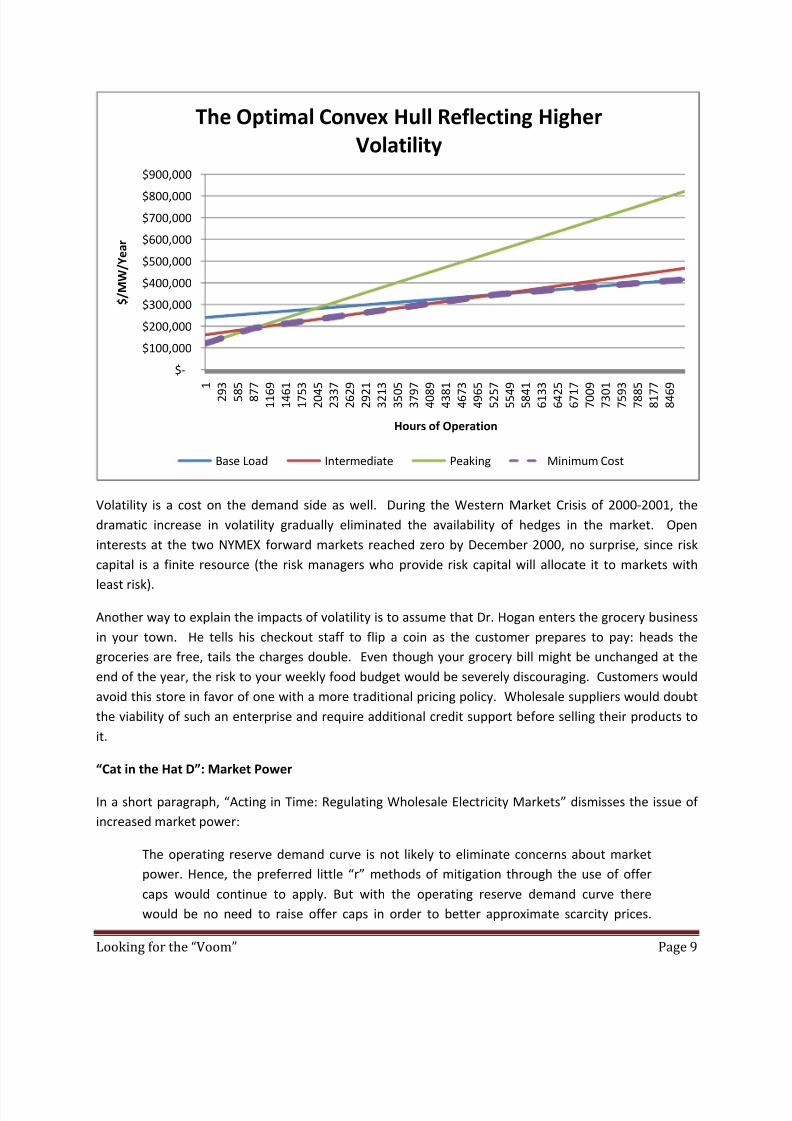
2. Dr. Hogan’s solution has a perceptible impact on the volatility of prices in the market. When the

market is allowed to operate without intervention, volatility is 58%. In Dr. Hogan’s improved

version, volatility has risen to 637%.10

3. Only a very ethical market participant would reject taking capacity offline when near system

peak. A “bump” in prices from $80/MWh to $10,000/MWh is likely to change market

participants’ behavior.11

Continuing my “Cat in the Hat” analogy, it is time for Cat in the Hats B, C, and D to appear.

“Cat in the Hat B”: Resource Optimality If we expect prices to lead to resource development, shifting the demand curve is a dangerous step. In

the final analysis, we would like to meet actual demand, not a hypothetical construction designed by

well‐meaning economists or bureaucrats. While we often forget past errors, it is wise to remember that

California’s PURPA misadventure was based on gerrymandering the price paid to PURPA developers –

resulting in a prolonged surplus and a massive rate shock for California’s ratepayers.12

As mentioned above, we can avoid the massive increase in market volatility by reducing the arbitrary

scarcity payment. Unfortunately, the producer’s surplus is effectively a rectangle. A lower operating

reserves price means an increase in the number of times the market must pay the reserves price. If we

reduce the price to $1,000/MWh, the expected hours the market will pay this increase slightly more

than tenfold. When there are more hours in which spot prices are greater than or equal to the peakers’

marginal cost, the further we depart from an optimal system.

“Cat in the Hat C”: Volatility Advocates of administered markets often neglect to address price volatility. Such volatility affects the

market

in

two

significant

ways.

First,

resource

developers

pay

more

for

capital

when

operating

in

a

volatile market. One reason why peakers are not a good choice in restructured markets is the difficulty

of convincing investors that profitability depends on a very few hours in the year.

Although Dr. Joskow’s example does not consider the capital cost implications of increasing price

volatility, it is not unlikely to assume that a peaker’s capital costs could increase by 50% when volatility

increases from 58% to 637%, especially when the change in volatility has been administered by a

regulatory agency. A change from $80,000/MW/Year to $120,000/MW/Year drives major changes in

the optimal resource portfolio, reducing peakers from 2,435 MW to 1,218 MW. The difference is made

up in more expensive intermediate resources.

10 In Dr. Hogan’s defense, the volatility is largely related to an arbitrary value of $10,000 used to price scarcity. As

the scarcity value is lowered, the volatility will decrease, but the departure from optimality will increase. 11

It is always wise to keep in mind Adam Smith’s sagacious comment that “People of the same trade seldom meet

together, even for merriment and diversion, but the conversation ends in a conspiracy against the public, or in

some contrivance to raise prices.” 12

A major motivation for California’s restructuring was the high prices caused by the high PURPA prices paid in the

1980s and early 1990s. While the prices were designed by the best technicians, the fact is that they were

considerably higher than they should have been.




Volatility is a cost on the demand side as well. During the Western Market Crisis of 2000‐2001, the

dramatic increase in volatility gradually eliminated the availability of hedges in the market. Open

interests at the two NYMEX forward markets reached zero by December 2000, no surprise, since risk

capital is a finite resource (the risk managers who provide risk capital will allocate it to markets with

least

risk).

Another way to explain the impacts of volatility is to assume that Dr. Hogan enters the grocery business

in your town. He tells his checkout staff to flip a coin as the customer prepares to pay: heads the

groceries are free, tails the charges double. Even though your grocery bill might be unchanged at the

end of the year, the risk to your weekly food budget would be severely discouraging. Customers would

avoid this store in favor of one with a more traditional pricing policy. Wholesale suppliers would doubt

the viability of such an enterprise and require additional credit support before selling their products to

it.

“Cat in the Hat D”: Market Power In a short paragraph, “Acting in Time: Regulating Wholesale Electricity Markets” dismisses the issue of

increased market power:

The operating reserve demand curve is not likely to eliminate concerns about market

power. Hence, the preferred little “r” methods of mitigation through the use of offer

caps would continue to apply. But with the operating reserve demand curve there

would be no need to raise offer caps in order to better approximate scarcity prices.

$‐

$100,000

$200,000

$300,000

$400,000

$500,000

$600,000

$700,000

$800,000

$900,000

1

2 9

3

5 8

5

8 7

7

1 1 6

9

1 4 6

1

1 7 5

3

2 0 4

5

2 3 3

7

2 6 2

9

2 9 2

1

3 2 1

3

3 5 0

5

3 7 9

7

4 0 8

9

4 3 8

1

4 6 7

3

4 9 6

5

5 2 5

7

5 5 4

9

5 8 4

1

6 1 3

3

6 4 2

5

6 7 1

7

7 0 0

9

7 3 0

1

7 5 9

3

7 8 8

5

8 1 7

7

8 4 6

9

$ / M W / Y e a r

Hours of Operation

The Optimal Convex Hull Reflecting Higher Volatility

Base Load Intermediate Peaking Minimum Cost




Unlike the plan in Texas and the practice in Australia, more realistic scarcity pricing

would not require higher or no limits on the offers by generators. Scarcity pricing would

be driven by the operating reserve demand curve and not solely by the generators’

offers. This would remove ambiguity from the analysis of high prices and distinguish

(inefficient) economic withholding through high offers from (efficient) scarcity pricing

derived from

the

operating

reserve

demand

curve.13

Having the market administrator meddle with prices will not remove ambiguity. The incentives that

scarcity pricing creates for market participants by themselves create ambiguity even before

implementing arbitrary shifts in the demand curve. The reality is that even smaller generators will

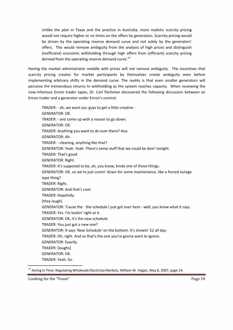
perceive the tremendous returns to withholding as the system reaches capacity. When reviewing the

now‐infamous Enron trader tapes, Dr. Carl Pechman discovered the following discussion between an

Enron trader and a generator under Enron’s control:

TRADER: ‐ ah, we want you guys to get a little creative ‐

GENERATOR: OK.

TRADER: ‐ and come up with a reason to go down.

GENERATOR: OK.

TRADER: Anything you want to do over there? Any‐

GENERATOR: Ah‐

TRADER: ‐ cleaning, anything like that?

GENERATOR: Yeah. Yeah. There's some stuff that we could be doin' tonight.

TRADER: That's good.

GENERATOR: Right.

TRADER: It's supposed to be, ah, you know, kinda one of those things.

GENERATOR:

OK,

so

we're

just

comin'

down

for

some

maintenance,

like

a

forced

outage

type thing?

TRADER: Right.

GENERATOR: And that's cool.

TRADER: Hopefully.

[they laugh]

GENERATOR: 'Cause the ‐ the schedule I just got over here ‐ well, you know what it says.

TRADER: Yes. I'm lookin' right at it.

GENERATOR: OK, it's the new schedule.

TRADER: You just got a new one?

GENERATOR: It

says

'New

Schedule'

on

the

bottom.

It's

showin'

52

all

day.

TRADER: Oh, right. And so that's the one you're gonna want to ignore.

GENERATOR: Exactly.

TRADER: [laughs]

GENERATOR: OK.

TRADER: Yeah. So‐





GENERATOR: We'll take care of that.

TRADER: So you got a ‐ so you're checkin' a switch on the steam turbine.

GENERATOR: Yeah, and whatever adjustment he makes today, is probably ‐ tonight, is

probably not gonna work, so we're probably gonna have to check it tomorrow

afternoon again.

TRADER: I think

that's

a good

plan,

Generator.

GENERATOR: All right.

TRADER: I knew I could count on you.

GENERATOR: No problem.14

This conversation reflects the fact that when near system peak, even a small generator can contribute to

a significant change in prices.

The following formula describes a generator’s calculation when a significant increase in prices is possible

due to a reduction in output:

(Scarcity Price–Marginal Cost) x (1–Withholding%) > Competitive Price–Marginal Cost

In Dr. Joskow’s example, shifting from $80/MWh to $10,000/MWh would meet this decision rule for

withholding at any level below 100% for peakers to a mere 99.4% for base load resources. The greater

the scarcity price imposed by market administrators, the greater the incentive for market participants to

“nudge” the market from competitive to scarcity pricing.

Looking for the “Voom” Unlike the Cat in the Hat, we can learn from history. Energy markets in the Western Interconnection

have

been

based

on

the

simple,

transparent

WSPP

model

since

the

1980s.

In

1994,

water

flows

and

reserves were low when the region suddenly suffered a major reliability disaster in the form of an

earthquake that leveled the southern terminus of the DC intertie. However, prices remained stable and

reflected underlying marginal costs, no emergency declarations were required, and the Western system

weathered the situation with few disruptions.

In 2000‐2001, substantially less exacting conditions created a situation during which California’s

Independent System Operator declared more than one hundred emergencies, and major industries in

the Pacific Northwest shut their doors forever. What was different?

1. California’s “Better Reliability Through Markets” turned out to be a poor method to purchase

capacity.

Restrictions on

the

options

available

to

the

California

ISO

(the

sole

buyer)

changed

the

ISO into a price taker in an extremely adverse market.

2. Availability of capacity from resources within CAISO’s service territory declined precipitously.

The five major merchant generators averaged a miserable 52% of capacity during the

emergency declarations in 2000 and 2001.

14 Docket EL03‐180 et al, Exhibit Snohomish 525, conversation between an Enron trader in Portland, Oregon, and

an employee of Las Vegas Cogeneration during a Stage 3 Emergency that CAISO declared in 2001.




3. Capacity responsibility suffered a significant “tragedy of the commons” where no one was

ultimately responsible for system reliability. We learned the hard way that an ISO has no

stockholders, no voters, and no regulators.

It is important to note that none of the problems California faced in 2000‐2001 took place in 1994. Yet in

1994,

the

efficient

WSPP

market

operated

without

governmental

intervention.

Because

capacity

requirements were decentralized, it would have been useless to maneuver capacity shortage

declarations through the use of Ricochets, Load Shifts, and suspicious forced outages.

Open markets in energy have existed in the United States for over twenty years. They have worked

transparently and efficiently. Intervening to “fix” them so as to approximate capacity markets is likely

both to fail and to create a host of follow‐on difficulties.

California’s experiences demonstrate that centralized capacity markets, especially those where rules

have been enacted to forbid purchasing capacity in an efficient manner, do not really work very well,

and are hugely expensive to implement, operate, and maintain.

”Voom” on the other hand is a laudable goal, and I believe that there are merits in retaining the “de” in

deregulation and in discouraging increased intervention in markets. Like the Cat in the Hat’s

shenanigans, Dr. Hogan’s solutions are interesting, but take us further away from competitive solutions.




Appendix: Why the Missing Money Problem affects all resource owners:

The convex hull identifies i vertices. Each vertice is the intersection between two lines: the ith total cost

line and i+1th total cost line. Total Cost(TC)=Fixed Costs(FC)+Hours of Operation(Hours)xVariable Cost

(VC). The intersection occurs at the number of hours where FCi+VCixHours=FCi+1+VCi+1xHours j.

We can solve for the Hours corresponding to each vertex on the optimal convex hull by collecting terms

and dividing. This gives Hours j=(FCi –FCi+1)/(VCi+1 –VCi).

A new resource will earn revenues towards its fixed cost only when prices are above its variable cost.

Another way to say this is that the most expensive resource will not expect to capture any producer’s

surplus since the highest price, at load resource balance, is just equal to its variable cost.

The next highest variable cost resource will receive a contribution towards its fixed cost when prices are

above its variable cost.

We can see this clearly using Dr. Joskow’s example:




In this example, peakers set the market prices for the highest load hours. Peakers’ owners will just

cover their variable costs during this period. Their expected loss is just equal to the fixed costs of a

peaker.

The intermediate resource owner fares better. Its producer’s surplus is equal to the red box.

Algebraically, the

size

of

this

box

is

(VCi

‐VCi+1)x

Vertex

1,

and

Vertex

1 is

(FCi –FCi+1)/(VCi+1 –VCi).

When

we

simplify the expression we find that the intermediate resource owners’ producer surplus is equal to FC2 –

FC1. The intermediate resource owners’ shortfall is just equal to the fixed cost of a peaker.

What about the next resource? The total producer’s surplus for each succeeding resource is equal to

the sum of the previous resource owner’s producer surplus plus the additional surplus provided by their

lower variable cost. In this case, the size of the red box is FC2 –FC1. The size of the green box is FC3 –FC2.

The sum of these two boxes is FC3 –FC1. The base load resource owner also has a shortfall of the fixed

cost of a peaker.

In the

general

case,

the

producer’s

surplus

of

resource

owner

i is

FC1 –FCi.

When

we

add

the

additional

revenues above variable cost for the next resource owner, they are FCi+1 –FCi so that the total producers’

surplus is FCi+1 –FC1.

A revenue shortfall is built into the energy only market for every resource owner regardless of the

number of different resource types in the analysis.

a rebuttal to dr. hogan: "looking for the 'voom'"

Documents