Discussion Papers in Economics

Discussion Paper

No. 11/04

A Regression Model for

the Copula Graphic Estimator

S.M.S. Lo and R.A. Wilke

April 2011

2011 DP 11/04

A Regression Model for the Copula Graphic Estimator.∗

Simon M.S. Lo†

Ralf A. Wilke‡

March 2011

∗Wilke is supported by the Economic and Social Research Council through the Bounds for Competing Risks

Duration Models using Administrative Unemployment Duration Data (RES-061-25-0059) grant.†Lingnan University, Rm 218, Ho Sin Hang Building, Lingnan University, Hong Kong, E–mail: si-

monlo@ln.edu.hk .‡University of Nottingham, School of Economics, University Park, Nottingham NG7 2RD, United Kingdom,

Phone: +441159515248, E–mail: ralf.wilke@nottingham.ac.uk

1

Abstract

We consider a dependent competing risks model with many risks and many covariates.

We show identifiability of the marginal distributions of latent variables for a given dependence

structure. Instead of directly estimating these distributions, we suggest a plug-in regression

framework for the Copula-Graphic estimator which utilises a consistent estimator for the

cumulative incidence curves. Our model is an attractive empirical approach as it does not

require knowledge of the marginal distributions which are typically unknown in applications.

We illustrate the applicability of our approach with the help of a parametric unemploy-

ment duration model with an unknown dependence structure. We construct identification

bounds for the marginal distributions and partial effects in response to covariate changes.

The bounds for the partial effects are surprisingly tight and often reveal the direction of the

covariate effect.

Keywords: Archimedean copula, dependent censoring

1 Motivation

The estimation of the marginal distribution, Fj, of a latent competing random variable Tj, is of

prime interest to determine causal relationships between a covariate and the time to an event. Fj

can be estimated directly by maximum likelihood techniques if it is known up to some unknown

coefficients and if the copula is known. Chen (2010) suggests a semiparametric transformation

model which includes the proportional odds and proportional hazard model as special cases. As a

drawback of this approach, direct estimation of Fj requires full or at least some knowledge about

Fj. Fj can be also determined with the Copula-Graphic estimator (Zheng and Klein, 1995). It

2

exploits a 1-1 relationship between the cumulative incidence curve for Tj, Qj, and Fj if the copula

is known. By using a nonparametric estimator for Qj it is possible to determine Fj, without having

any prior knowledge about it. As an important limitation, this approach was not yet extended to

a model with many covariates. Braekers and Veraverbeke (2005) consider a nonparametric model

with one continuous covariate but to our knowledge a general regression framework for multiple

covariates has still to be developed.

This paper closes this gap by suggesting a multiple regression model for the Copula-Graphic

estimator. We are able to establish a direct link between a multivariate Qj and Fj conditional

to many covariates. Our approach works with any consistent estimator for Qj and is therefore

not restricted to specific subdistribution models. Special cases of our model therefore include

semiparametric (Fine and Gray, 1999) or parametric models (Jeong and Fine, 2007) for Qj. We

elaborate in detail a parametric regression model for which we derive a closed form solution for Fj

and its asymptotic covariance matrix. In particular, we consider a parametric maximum likelihood

estimator for Qj. This model includes the proportional odds and proportional hazard model with

Gompertz baseline function as special cases (Jeong and Fine, 2007). We claim that our approach

is appealing for empirical research as it does not impose direct restrictions on Fj which would be

difficult to test. Instead, it impose restrictions on Qj which can be directly verified by data. Our

implementation of the estimation approach is fast as it is based on closed form solutions. STATA

code is available on request from the first author. We demonstrate the applicability by means of a

parametric unemployment duration model. As the dependence structure between risks is unknown

in this example, we construct bounds for Sj = 1 − Fj which are due to the non-identifiability of

the competing risks model. Moreover, we construct bounds for partial effects on Sj in response

to covariate changes. We find that these bounds are rather tight in our example and estimation

3

results are often informative about the sign of a covariate effect.

The next section considers the general model. In Section 3 we derive closed form expressions

for the parametric model. Section 4 presents an application to unemployment duration data and

the last section provides a final discussion.

2 The Model

We consider a model with j = 1, . . . , J competing random variables Tj ∈ IR+ with an unknown

marginal distribution function Fj(t;x) = pr(Tj ≤ t;x) ∈ [0, 1] and marginal survival function

Sj(t;x) = 1− Fj(t;x). x ∈ IRK is a K × 1 vector of observable covariates. Due to the competing

risks structure it is only possible to observe (T, δ,x) with δ = argminj{Tj} and T = minj{Tj}.

Let (Ti, δi,xi) be i = 1, . . . , N realisations of (T, δ,x) and Qj(t) = pr(Tj ≤ t, δ = j;x) be

the cumulative incidence curve for risk j = 1, . . . , J . The cause specific hazard is hj(t;x) =

lim∆t→0(1/∆t)pr{t ≤ T ≤ t+∆t, δ = j|T ≥ t,x} = Q′j(t;x)/S(t;x) with Q

′(t;x) = dQj(t;x)/dt.

S(t;x) = pr(T ≥ t;x) is the survival function of the minimum.

Zheng and Klein (1995) show that Sj can be identified if the copula, C(S1, . . . , SJ) with

coefficients ω, is known. Their approach, known as the Copula-Graphic estimator, is restricted to

a model with J = 2 and without x. Lo and Wilke (2010) generalize the Copula-Graphic estimator

to J > 2 if the copula is Archimedean. Given Qj(t) for all j and S(t), Sj(t) can be determined by

solving a system of equations. In this paper we suggest a regression setting for the copula graphic

estimator which does not restrict the number of risks nor the number of covariates. We therefore

develop a regression setting for Sj(t;x) given Qj(t;x) and C(.).

In the regression setting, Sj(t;x) can be identified using two approaches: First, it is possible to

specify the joint likelihood function if C(.) is known, and Sj(t;x) belongs to a known parametric

4

or semiparametric family with unknown coefficients ψj for all j. For the purpose of illustration,

we sketch the likelihood function for a two risks model:

L(ψ1, ψ2) =N∏i=1

pr(T1i = t, T2i > t,xi)1I{δi=1}pr(T1i > t, T2i = t,xi)

1I{δi=2}

=N∏i=1

2∏j=1

∂

∂Sj

C{S1(Ti;xi;ψ1), S2(Ti;xi;ψ2)}1I{δi=j} .

For fully specified S1(t;x;ψ1) and S2(t;x;ψ2), standard methods can be applied to estimate the

unknown coefficients by maximising L(.). Chen (2010) considers the case when S1(t;x;ψ1) and

S2(t;x;ψ2) belong to a semiparametric transformation model which includes the proportional

hazard and the proportional odds models as special cases. Nonparametric maximum likelihood

estimators are applied to solve for the unknown coefficients. Note that direct specification of the

joint distribution is not an extension of the copula graphic estimator. The main idea of the copula

graphic estimator is that the marginal survival function can be identified without imposing any

direct parametric or semiparametric structure on them.

The second approach is to generalise the Copula-Graphic estimator to a model with covariates.

We are only aware of one such attempt. Braekers and Veraverbeke (2005) use nonparametric

kernel estimators for Fj(t;x) but their approach is limited to K = 1. In this paper we extend the

Copula-Graphic estimator to a regression model with many covariates.

Identifiability We require two regularity conditions for the copula to show identifiability of the

unknown Sj(t;x) for known Qj(t, ;x) and known or assumed C(S1, . . . , SJ).

Assumption 1 C(S1, . . . , SJ) has the following properties:

1. It is Archimedean;

2. C(S1, . . . , SJ) = C(S1, . . . , SJ ,x).

5

Then

C(s1, . . . , sJ) = ϕ−1[ϕ{S1(t;x)}, . . . , ϕ{SJ(t;x)}]

with ϕ(S) : [0, 1] → IR+ is the so called copula generator. ϕ is a strictly decreasing and twice

differentiable continuous function with ϕ(1) = 0.

Proposition 1 Sj(t;x) is identified under Assumption 1 if Qj(t;x) is known for all j. There

exists a closed form solution

Sj(t;x) = ϕ−1

[−∫ t

0

ϕ′{S(u;x)}S(u;x)hj(u;x)du]

(1)

= ϕ−1

[−∫ t

0

ϕ′(1−J∑

j=1

Qj(u;x))Q′j(u;x)du

]= Ψj(Q(t;x)).

with Q(t;x) = (Q1(t;x), . . . , QJ(t;x))′.

See Appendix 1 for the proof. This result is a generalization of equation (7) in Rivest and

Wells (2001) for a two risks model in absence of covariates. Qj can be directly estimated from

data without specifying the copula function. It therefore differs from the common approach to

identification of the competing risks models which directly specifies and estimates Sj(t;x). We

claim that it is easier to check the specification of Qj(t;x) as it describes an observed rather than

a latent quantity. It is therefore easier to verify consistent estimation of Qj(t;x) in an application

than verifying the consistency conditions for direct estimation of Sj(t;x). Our approach reverses

the approach of Cheng, Fine and Wei (1998) who first estimate a model for Sj(t;x) and then

predict Qj(t;x).

Estimation and large sample properties Equation (1) forms the basis of our model for es-

timating Sj(t;x). Since C(.) is known, the right hand side is nothing else than a known function

6

of Qj(t;x) as S(t;x) = 1−∑J

j=1Qj(t;x) and hj(t;x) = Q′j(t;x)/S(t;x). It is therefore straight-

forward to estimate Sj(t;x) by Sj(t;x) in a second stage after Qj(t;x) was first estimated by

Qj(t;x):

Sj(t;x) = ϕ−1

[−∫ t

0

ϕ′{S(u;x)}S(u;x)hj(u;x)du], (2)

where S(t;x) = 1 −∑J

j=1 Qj(t;x) and hj(t;x) = Q′j(t;x)/S(t;x). The model is very general

as Qj(t;x) can be nonparametric, semiparametric or parametric. In any case the large sample

properties of Qj(t;x) determine the large sample properties of Sj(t;x) something that is elaborated

in more detail below. If Qj(t;x) is parametric, there may be an analytical solution to equation

(1) (see also next section) otherwise it is be obtained my means of numerical methods. The same

is true for the marginal effect of say xk on Sj(t;x) which is ∂Sj(t;x)/∂x. The marginal effect is

often of prime interest in applications.

Proposition 2 Suppose Qj(t;x) converges in probability to Qj(t;x) for all j and Q(t;x) converges

to a distribution with J × J covariance matrix ΣQ. Then under Assumption 1, we have:

1. Sj(t;x) converges in probability to Sj(t;x), and

2. Sj(t;x) has asymptotic variance

var(Sj) = [Ψ′j(Q(t;x))]′ΣQ[Ψ

′j(Q(t;x))]

with Ψ′j(Q(t;x)) = ∂Ψj(Q(t;x))/∂Q(t;x) is J × 1.

The consistency result is an immediate consequence of the Continuous Mapping Theorem (Van der

Vaart, 1998, Theorem, 2.3) provided that Ψ is continuous due to Assumption 1. The distribution

can be obtained by a direct application of the Delta Method (Van der Vaart, 1998, Theorem, 3.1)

provided that Ψ is differentiable due to Assumption 1.

7

3 Parametric Example

Let us now assume that Qj(t) = pr(Tj ≤ t, δ = j;x) for j = 1, . . . , J is known up to some

coefficients Θj ∈ RL with L ≥ K. Recent work for such a model include Jeong and Fine (2007)

and Peng and Fine (2009) or Lambert (2007). As an example we use a direct parametric modeling

approach for Qj. In particular, we specify an odds rate transformation model with Gompertz

distribution as the improper baseline subdistribution (Jeong and Fine, 2007). In this model

Qj(t;x) = 1− [1 + αjτj exp(x′βj){exp(ρjt)− 1}/ρj]−1/αj . (3)

is known up to Θj = {β′j, ρj, αj, lτj}′ with ρj ∈ IR and τj = exp(lτj) ∈ IR+ as the parameters

of the Gompertz distribution and αj ∈ IR and βj ∈ IRK as the parameters of the transformation

model. The cause specific hazard of risk j is

hj(t;x) =Bj exp(−Aj(1 + αj)/αj)∑Jj=1 exp(−Aj/αj)− J + 1

with

Aj = ln[1 + αjτj exp(x′βj){exp(ρjt)− 1}/ρj];

Bj = τj exp(x′βj) exp(ρjt).

This model encompasses the proportional odds (αj = 1) and the proportional hazard model

(αj → 0) with Gompertz baseline as special cases. Even though by being rather general for a

parametric model, it restricts the subdistribution hazard to be monotonic in t.

As the copula function we assume the Frank copula.

Remark 1 The Frank copula has the following properties:

ϕ(t) = − ln

[exp(−ωt)− 1

exp(−ω)− 1

]; ϕ′(t) =

ω exp(−ωt)exp(−ωt)− 1

;

ϕ−1(u) = − 1

ωln[exp(−u){exp(−ω)− 1}+ 1] ; ϕ′−1(u) =

exp(−u){exp(−ω)− 1}ω[exp(−u){exp(−ω)− 1}+ 1]

8

with ω ∈ (−∞,∞) \ {0}.

When ω = 0, we have ϕ(t) = −ln(t). In what follows we derive closed form expressions

for Sj(t;x) and the marginal effect ∂Sj(t;x)/∂xk for given values of Θj and for ω /∈ 0. For

notational convenience we consider a two risks model as it is always possible to apply the risk

pooling approach of Lo and Wilke (2010) if the copula is Archimedean. In this case the first risk

is of direct interest and second is the minimum of all other risks which does not have a direct

interpretation.

First note that

S(t;x) = exp(−A1/α1) + exp(−A2/α2)− 1; (4)

Q′j(t;x) = Bj exp{−Aj(1 + 1/αj)}. (5)

By plugging (4) and (5) into (1), we obtain a closed form solution for the latent marginal distri-

bution:

Sj(t;x) = ϕ−1[−Ij(t;x)], (6)

where

Ij(t;x) =

∫ t

0

Dj(u;x)du; and (7)

Dj(t;x) = ϕ′(S(t;x))Q′j(t;x) =

ω exp[−ωS(t;x)]exp[−ωS(t;x)]− 1

Q′j(t;x). (8)

Equation (6) suggests that imposing parametric structure on Qj(t;x) implies some shape restric-

tions for Sj(t;x). As the functional form of Sj is non trivial, the interpretation of βj is unclear.

To study the effect of a change in x on the survival probability it is possible to compute Sj(t;x)

for different values of x and to compare the resulting probabilities. For a continuous covariate it

9

is also possible to consider the marginal effect which is

∂Sj(t;x)/∂xk = −ϕ′−1{−Ij(t,x)}∂Ij(t,x)

∂xk(9)

where

∂Ij(t,x)/∂xk =

∫ t

0

∂Dj(u;x)

∂xkdu, (10)

and

∂Dj(t;x)/∂xk = Q′j

∂ϕ′{S(t;x)}∂xk

+∂Q′

j

∂xkϕ′{S(t;x)};

which can be solved by replacing

∂ϕ′{S(t;x)}/∂xk =ω2 exp(−ωS(t;x))

{exp(−ωS(t;x))− 1}2∂S(t;x)

∂xk;

∂S(t;x)/∂xk = −∑j

exp(−Aj/αj)

αj

{1− exp(−Aj)}βjk;

∂Q′j(t;x)/∂xk = [1− (1 + 1/αj)(1− exp(−Aj))]Q

′jβjk.

Note that ∂Aj/∂xk = {1− exp(−Aj)}βjk and ∂Bj/∂xk = Bjβjk.

It is apparent that the marginal effect (9) depends on t and x in a non trivial way. In our

practical work with the model we have seen cases where the sign of the marginal effect changes in

t. The parametric model (3) for Qj therefore does not imply a non crossing property for marginal

survival curves as it is assumed in the proportional hazards model for Sj. In an application

the marginal effect may be determined at the sample mean of the covariates or as the average

population marginal effect (AME) which is AME = N−1∑N

i=1 ∂Sj(t;xi)/∂xk.

Estimation and large sample properties The unknown coefficients Θj for j = 1, 2 in (3)

can be directly estimated by parametric maximum likelihood (Jeong and Fine, 2007). In this case

10

Θ = (Θ1, Θ2)′ is consistent and asymptotically normal with known asymptotic covariance matrix.

The estimator for Sj(t;x) is a plug in solution to (2).

As this model is a special case of the model considered in Section 2, we know that the estimator

for Sj(t;x) is also consistent and asymptotically normal. In the following we derive a closed form

for its asymptotic variance. First note that the asymptotic variance of Qj(t;x) = Qj(t;x, Θj) is

(Jeong and Fine, 2007)

ΣQj=

[∂Q(t;x)

∂Θ′j

]ΣΘj

[∂Q(t;x)

∂Θ′j

]′, (11)

with ΣΘjas the covariance matrix of Θj. For simplicity let us consider a two risks model (J = 2)

but this can be easily extended to J > 2 under Assumption 1. Then, let S = (S1, S2)′ and

∂S(t;x)/∂x = (∂S1(t;x)/∂x, ∂S2(t;x)/∂x)′ with the latter being a 2K × 1 matrix. As the

marginal distributions and the marginal effects are nonlinear functions of Q(t;x) we can write

S(t;x) = Ψ(Q(t;x)) = Ψ∗(t;x, Θ) (12)

∂S(t;x)/∂x = Ξ(Q(t;x)) = Ξ∗(t;x, Θ). (13)

Due to the consistency of S we can focus on its asymptotic distribution with Θ = Θ|Θ0 and Θ0

being the true value of Θ. The asymptotic covariance matrices of S(t;x) and ∂S(t;x)/∂x are

ΣS(t;x) =

[∂Ψ∗(t;x,Θ)

∂Θ′

]ΣΘ

[∂Ψ∗(t;x,Θ)

∂Θ′

]′; (14)

Σ∂S(t;x)/∂x =

[∂Ξ∗(t;x,Θ)

∂Θ′

]ΣΘ

[∂Ξ∗(t;x,Θ)

∂Θ′

]′, (15)

with ΣΘ as the covariance matrix of Θ. We show in Appendix 2 that there are closed form solu-

tions for all right hand side components in (14) and (15).

11

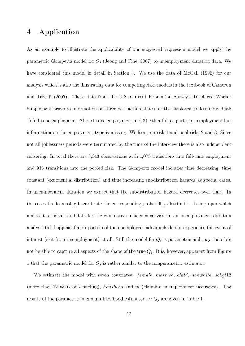
4 Application

As an example to illustrate the applicability of our suggested regression model we apply the

parametric Gompertz model for Qj (Jeong and Fine, 2007) to unemployment duration data. We

have considered this model in detail in Section 3. We use the data of McCall (1996) for our

analysis which is also the illustrating data for competing risks models in the textbook of Cameron

and Trivedi (2005). These data from the U.S. Current Population Survey’s Displaced Worker

Supplement provides information on three destination states for the displaced jobless individual:

1) full-time employment, 2) part-time employment and 3) either full or part-time employment but

information on the employment type is missing. We focus on risk 1 and pool risks 2 and 3. Since

not all joblessness periods were terminated by the time of the interview there is also independent

censoring. In total there are 3,343 observations with 1,073 transitions into full-time employment

and 913 transitions into the pooled risk. The Gompertz model includes time decreasing, time

constant (exponential distribution) and time increasing subdistribution hazards as special cases.

In unemployment duration we expect that the subdistribution hazard decreases over time. In

the case of a decreasing hazard rate the corresponding probability distribution is improper which

makes it an ideal candidate for the cumulative incidence curves. In an unemployment duration

analysis this happens if a proportion of the unemployed individuals do not experience the event of

interest (exit from unemployment) at all. Still the model for Qj is parametric and may therefore

not be able to capture all aspects of the shape of the true Qj. It is, however, apparent from Figure

1 that the parametric model for Qj is rather similar to the nonparametric estimator.

We estimate the model with seven covariates: female, married, child, nonwhite, schgt12

(more than 12 years of schooling), houshead and ui (claiming unemployment insurance). The

results of the parametric maximum likelihood estimator for Qj are given in Table 1.

12

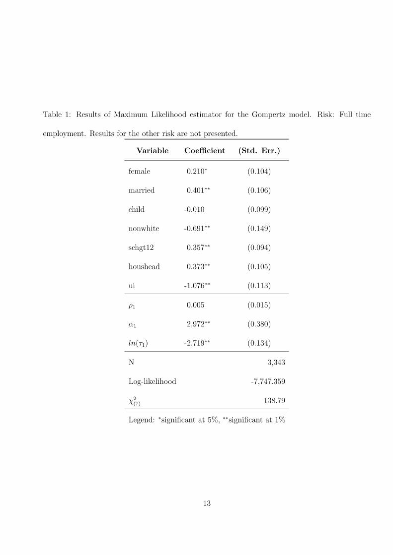
Table 1: Results of Maximum Likelihood estimator for the Gompertz model. Risk: Full time

employment. Results for the other risk are not presented.

Variable Coefficient (Std. Err.)

female 0.210∗ (0.104)

married 0.401∗∗ (0.106)

child -0.010 (0.099)

nonwhite -0.691∗∗ (0.149)

schgt12 0.357∗∗ (0.094)

houshead 0.373∗∗ (0.105)

ui -1.076∗∗ (0.113)

ρ1 0.005 (0.015)

α1 2.972∗∗ (0.380)

ln(τ1) -2.719∗∗ (0.134)

N 3,343

Log-likelihood -7,747.359

χ2(7) 138.79

Legend: ∗significant at 5%, ∗∗significant at 1%

13

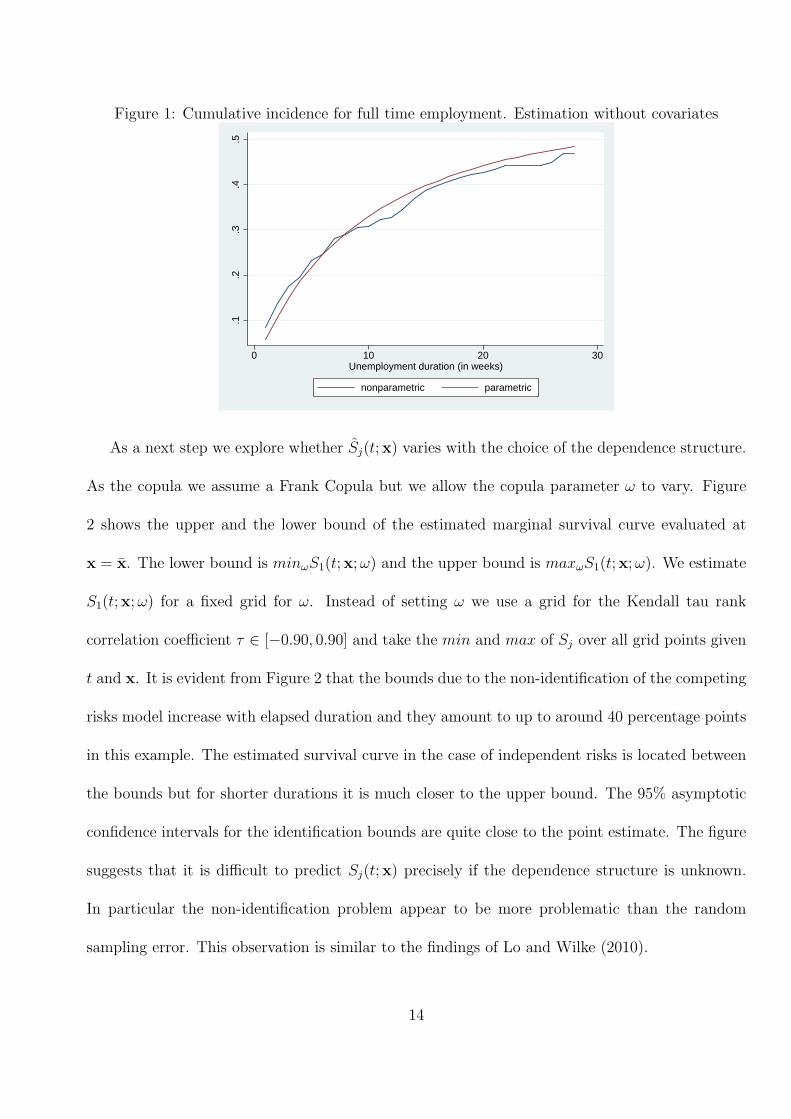
Figure 1: Cumulative incidence for full time employment. Estimation without covariates

.1.2

.3.4

.5

0 10 20 30Unemployment duration (in weeks)

nonparametric parametric

As a next step we explore whether Sj(t;x) varies with the choice of the dependence structure.

As the copula we assume a Frank Copula but we allow the copula parameter ω to vary. Figure

2 shows the upper and the lower bound of the estimated marginal survival curve evaluated at

x = x. The lower bound is minωS1(t;x;ω) and the upper bound is maxωS1(t;x;ω). We estimate

S1(t;x;ω) for a fixed grid for ω. Instead of setting ω we use a grid for the Kendall tau rank

correlation coefficient τ ∈ [−0.90, 0.90] and take the min and max of Sj over all grid points given

t and x. It is evident from Figure 2 that the bounds due to the non-identification of the competing

risks model increase with elapsed duration and they amount to up to around 40 percentage points

in this example. The estimated survival curve in the case of independent risks is located between

the bounds but for shorter durations it is much closer to the upper bound. The 95% asymptotic

confidence intervals for the identification bounds are quite close to the point estimate. The figure

suggests that it is difficult to predict Sj(t;x) precisely if the dependence structure is unknown.

In particular the non-identification problem appear to be more problematic than the random

sampling error. This observation is similar to the findings of Lo and Wilke (2010).

14

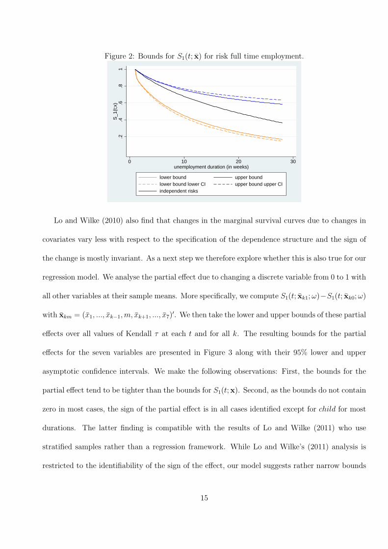
Figure 2: Bounds for S1(t; x) for risk full time employment.

.2.4

.6.8

1S

_1(t

;x)

0 10 20 30unemployment duration (in weeks)

lower bound upper boundlower bound lower CI upper bound upper CIindependent risks

Lo and Wilke (2010) also find that changes in the marginal survival curves due to changes in

covariates vary less with respect to the specification of the dependence structure and the sign of

the change is mostly invariant. As a next step we therefore explore whether this is also true for our

regression model. We analyse the partial effect due to changing a discrete variable from 0 to 1 with

all other variables at their sample means. More specifically, we compute S1(t; xk1;ω)−S1(t; xk0;ω)

with xkm = (x1, ..., xk−1,m, xk+1, ..., x7)′. We then take the lower and upper bounds of these partial

effects over all values of Kendall τ at each t and for all k. The resulting bounds for the partial

effects for the seven variables are presented in Figure 3 along with their 95% lower and upper

asymptotic confidence intervals. We make the following observations: First, the bounds for the

partial effect tend to be tighter than the bounds for S1(t;x). Second, as the bounds do not contain

zero in most cases, the sign of the partial effect is in all cases identified except for child for most

durations. The latter finding is compatible with the results of Lo and Wilke (2011) who use

stratified samples rather than a regression framework. While Lo and Wilke’s (2011) analysis is

restricted to the identifiability of the sign of the effect, our model suggests rather narrow bounds

15

for the magnitude. The results in Figure 3 also provide evidence that the estimated partial effect

is often statistically significant. Third, although the bounds for the partial effect for child contain

zero, we observe that the direction of the effect actually changes with elapsed duration for a given

ω. As the position of the sign change varies with ω, the bounds in Figure 3(c) contain the value

zero for most durations. A change in the direction of a covariate effect would not be obtained when

directly fitting a proportional hazards model for the marginal distribution which would assume

non-crossing of marginal survival curves.

16

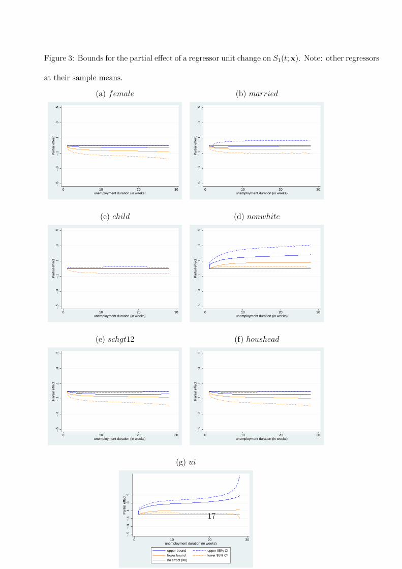
Figure 3: Bounds for the partial effect of a regressor unit change on S1(t;x). Note: other regressors

at their sample means.

(a) female (b) married

−.5

−.3

−.1

.1.3

.5P

artia

l effe

ct

0 10 20 30unemployment duration (in weeks)

−.5

−.3

−.1

.1.3

.5P

artia

l effe

ct

0 10 20 30unemployment duration (in weeks)

(c) child (d) nonwhite

−.5

−.3

−.1

.1.3

.5P

artia

l effe

ct

0 10 20 30unemployment duration (in weeks)

−.5

−.3

−.1

.1.3

.5P

artia

l effe

ct

0 10 20 30unemployment duration (in weeks)

(e) schgt12 (f) houshead

−.5

−.3

−.1

.1.3

.5P

artia

l effe

ct

0 10 20 30unemployment duration (in weeks)

−.5

−.3

−.1

.1.3

.5P

artia

l effe

ct

0 10 20 30unemployment duration (in weeks)

(g) ui

−.5

−.3

−.1

.1.3

.5P

artia

l effe

ct

0 10 20 30unemployment duration (in weeks)

upper bound upper 95% CIlower bound lower 95% CIno effect (=0)

17

5 Discussion

We suggest a regression framework for the copula graphic estimator and therefore extend the model

of Zheng and Klein (1995) and Lo and Wilke (2010) to many covariates. Under mild conditions

we show identifiability and derive nice asymptotic properties for our framework. Our approach

utilises direct estimates of the cumulative incidence curves which are identifiable quantities. It is

therefore easier to verify the specification of the estimator than for estimating latent quantities.

The only crucial assumption is that the model requires knowledge of the dependence structure

between risks. In an application with unknown dependence structure, however, it is easy to create

bounds for values of interest which represent the effect of the choice of the dependence structure.

In our illustrative application of a parametric model to unemployment duration data we obtain

that these bounds for partial effects are rather narrow while the bounds for the latent marginal

distributions are wide. The results of our application therefore suggest that it is possible to obtain

conclusive information about the effect of covariates even if the dependence structure is unknown.

18

References

[1] Braekers, R. and Veraverbeke, N. (2005) A copula-graphic estimator for the conditional survival

function under dependent censoring, Canadian Journal of Statistics, 33, 429–447.

[2] Cameron, A.C., and Trivedi, P.K. (2005)Microeconometrics, Cambridge University Press, New

York.

[3] Chen, Y.H. (2010) Semiparametric marginal regression analysis for dependent competing risks

under an assumed copula, Journal of the Royal Statistical Society B, 72, 235–231.

[4] Cheng, S.C., Fine, J.P. and Wei, L.J (1998) Prediction of Cumulative Incidence Function under

the Proportional Hazards Model, Biometrics, 54, 219–228.

[5] Fine, J.P. and Gray, R.J. (1999) A Proportional Hazards Model for the Subdistribution of a

Competing Risk, Journal of the American Statistical Association, 94, 496–509.

[6] Jeong, J.H. and Fine, J.P. (2007) Parametric regression on cumulative incidence function,

Biostatistics, 8, 1–13.

[7] Lambert, P.C. (2007) Modelling of the Cure Fraction in Survival Studies, The Stata Journal,

7, 351–375.

[8] Lo, S.M.S. and Wilke, R.A. (2010), A copula model for dependent competing risks, Journal

of the Royal Statistical Society Series C, 59, 359–376.

[9] Lo, S.M.S. and Wilke, R.A. (2011), Identifiability and estimation of the sign of a covariate

effect in the competing risks model, mimeo.

19

[10] McCall, B.P. (1996) Unemployment Insurance Rules, Joblessness, and Part-Time Work,

Econometrica, 64, 647–682.

[11] Rivest, L. and Wells, M.T. (2001) A Martingale Approach to the Copula-Graphic Estimator

for the Survival Function under Dependent Censoring, Journal of Multivariate Analysis, 79,

138–155.

[12] Van der Vaart, A.W. (1998), Asymptotic Statistics, Cambridge University Press, Cambridge.

[13] Zheng, M. and Klein, J.P. (1995), Estimates of marginal survival for dependent competing

risks based on assumed copula. Biometrika, 82, 127–138.

Appendix 1

Proof of Proposition 1. For notational simplicity we present the case J = 2. The cause-specific

hazard can be written as

h1(t) =pr(T1 = t, T2 ≥ t)

pr(T1 ≥ t, T2 ≥ t)=

− ∂∂upr(T1 ≥ u, T2 ≥ v)|v=u

pr(T1 ≥ t, T2 ≥ t)

= −∂S1(t)

∂t

∂C

∂S1

1

S(t)

When differentiating ϕ{S(t)} = ϕ{S1(t)}+ ϕ{S2(t)} with respect to S1 we obtain

ϕ′{S(t)} ∂C∂S1

= ϕ′{S1(t)}.

We obtain (1) when combining the two above results:

ϕ{Sj(t)} =

∫ t

0

ϕ′{S(u)}S(u)∂S1(u)

∂u

ϕ′{S1(u)}ϕ′{S(u)}

1

S(u)du

=

∫ t

0

ϕ′{S1(u)} dS1(u).

20

Appendix 2

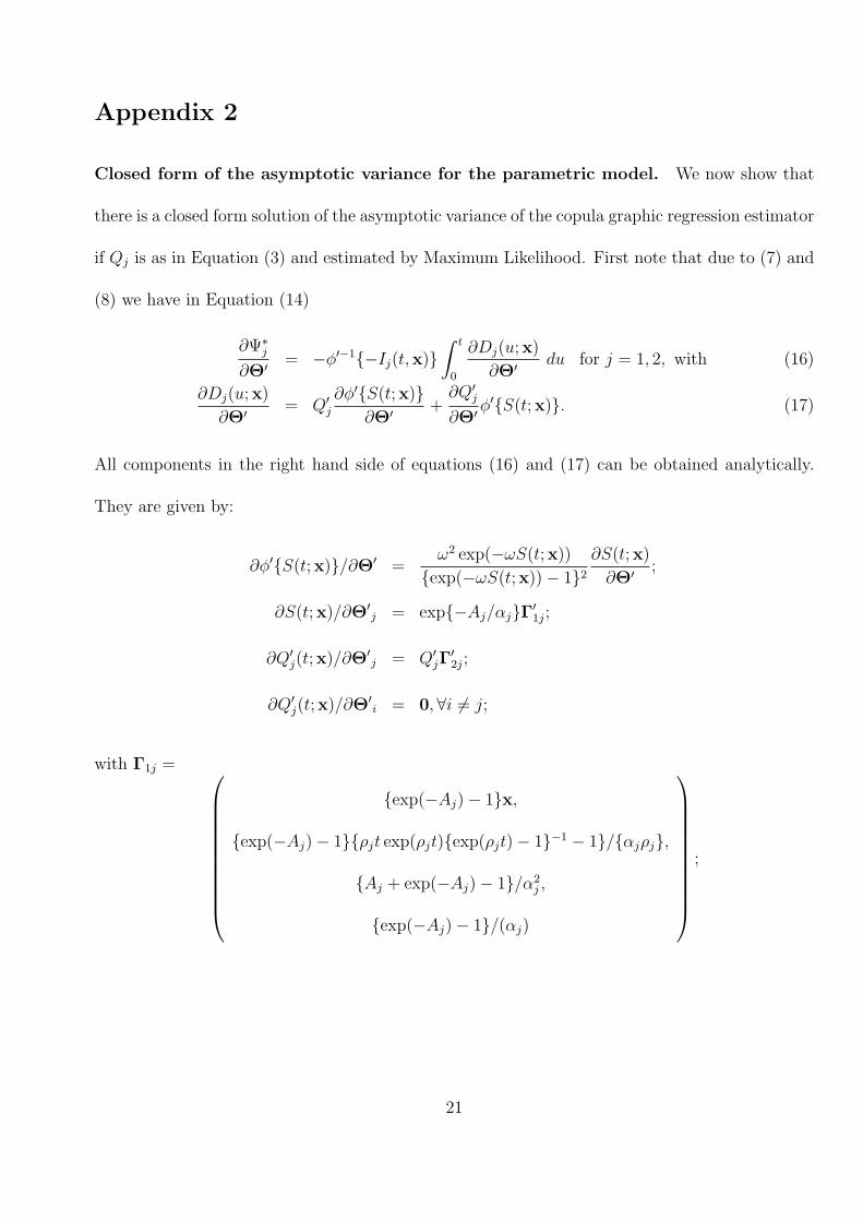
Closed form of the asymptotic variance for the parametric model. We now show that

there is a closed form solution of the asymptotic variance of the copula graphic regression estimator

if Qj is as in Equation (3) and estimated by Maximum Likelihood. First note that due to (7) and

(8) we have in Equation (14)

∂Ψ∗j

∂Θ′ = −ϕ′−1{−Ij(t,x)}∫ t

0

∂Dj(u;x)

∂Θ′ du for j = 1, 2, with (16)

∂Dj(u;x)

∂Θ′ = Q′j

∂ϕ′{S(t;x)}∂Θ′ +

∂Q′j

∂Θ′ϕ′{S(t;x)}. (17)

All components in the right hand side of equations (16) and (17) can be obtained analytically.

They are given by:

∂ϕ′{S(t;x)}/∂Θ′ =ω2 exp(−ωS(t;x))

{exp(−ωS(t;x))− 1}2∂S(t;x)

∂Θ′ ;

∂S(t;x)/∂Θ′j = exp{−Aj/αj}Γ′

1j;

∂Q′j(t;x)/∂Θ

′j = Q′

jΓ′2j;

∂Q′j(t;x)/∂Θ

′i = 0,∀i = j;

with Γ1j =

{exp(−Aj)− 1}x,

{exp(−Aj)− 1}{ρjt exp(ρjt){exp(ρjt)− 1}−1 − 1}/{αjρj},

{Aj + exp(−Aj)− 1}/α2j ,

{exp(−Aj)− 1}/(αj)

;

21

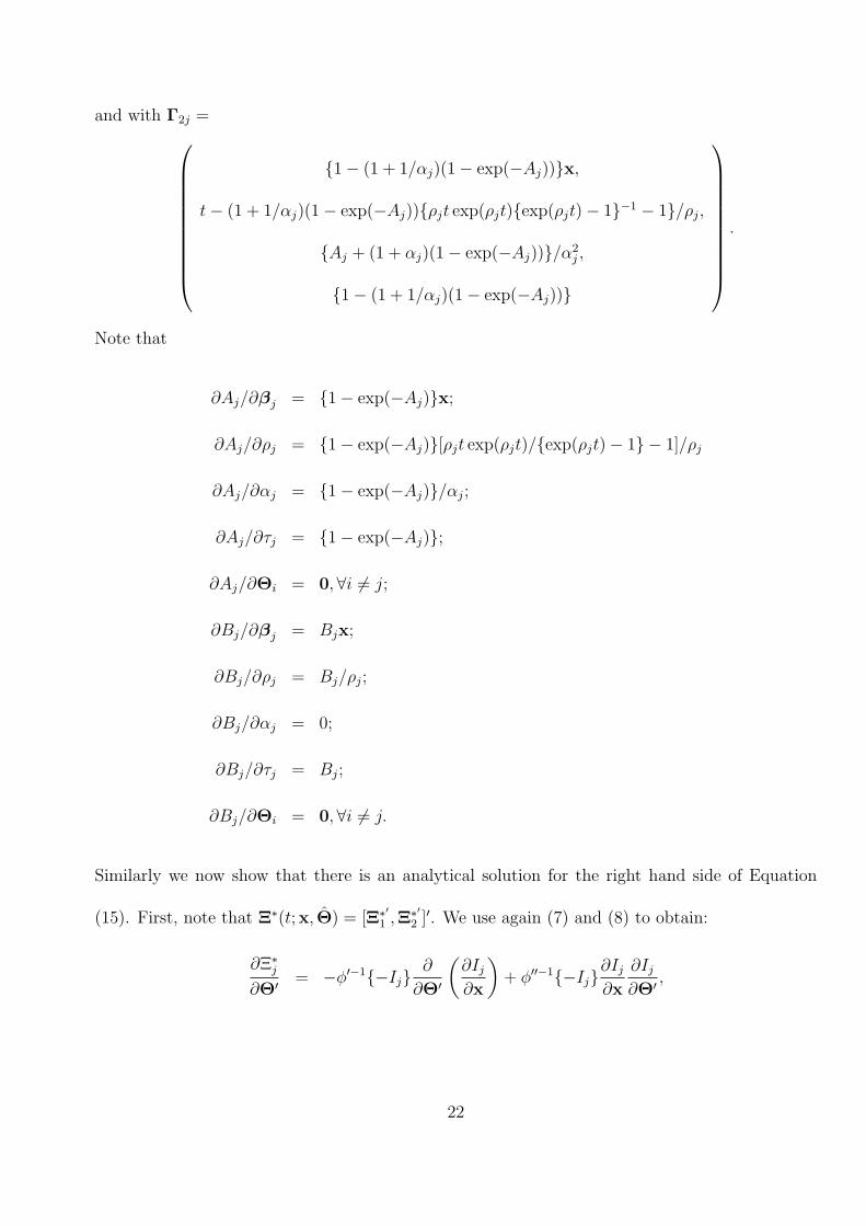
and with Γ2j =

{1− (1 + 1/αj)(1− exp(−Aj))}x,

t− (1 + 1/αj)(1− exp(−Aj)){ρjt exp(ρjt){exp(ρjt)− 1}−1 − 1}/ρj,

{Aj + (1 + αj)(1− exp(−Aj))}/α2j ,

{1− (1 + 1/αj)(1− exp(−Aj))}

.

Note that

∂Aj/∂βj = {1− exp(−Aj)}x;

∂Aj/∂ρj = {1− exp(−Aj)}[ρjt exp(ρjt)/{exp(ρjt)− 1} − 1]/ρj

∂Aj/∂αj = {1− exp(−Aj)}/αj;

∂Aj/∂τj = {1− exp(−Aj)};

∂Aj/∂Θi = 0,∀i = j;

∂Bj/∂βj = Bjx;

∂Bj/∂ρj = Bj/ρj;

∂Bj/∂αj = 0;

∂Bj/∂τj = Bj;

∂Bj/∂Θi = 0,∀i = j.

Similarly we now show that there is an analytical solution for the right hand side of Equation

(15). First, note that Ξ∗(t;x, Θ) = [Ξ∗′1 ,Ξ

∗′2 ]

′. We use again (7) and (8) to obtain:

∂Ξ∗j

∂Θ′ = −ϕ′−1{−Ij}∂

∂Θ′

(∂Ij∂x

)+ ϕ′′−1{−Ij}

∂Ij∂x

∂Ij∂Θ′ ,

22

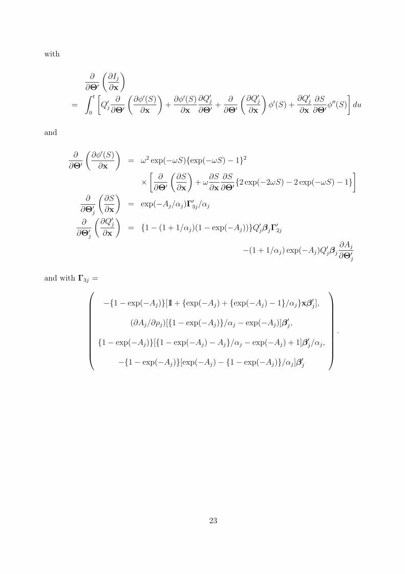
with

∂

∂Θ′

(∂Ij∂x

)=

∫ t

0

[Q′

j

∂

∂Θ′

(∂ϕ′(S)

∂x

)+∂ϕ′(S)

∂x

∂Q′j

∂Θ′ +∂

∂Θ′

(∂Q′

j

∂x

)ϕ′(S) +

∂Q′j

∂x

∂S

∂Θ′ϕ′′(S)

]du

and

∂

∂Θ′

(∂ϕ′(S)

∂x

)= ω2 exp(−ωS){exp(−ωS)− 1}2

×[∂

∂Θ′

(∂S

∂x

)+ ω

∂S

∂x

∂S

∂Θ′{2 exp(−2ωS)− 2 exp(−ωS)− 1}]

∂

∂Θ′j

(∂S

∂x

)= exp(−Aj/αj)Γ

′3j/αj

∂

∂Θ′j

(∂Q′

j

∂x

)= {1− (1 + 1/αj)(1− exp(−Aj))}Q′

jβjΓ′2j

−(1 + 1/αj) exp(−Aj)Q′jβj

∂Aj

∂Θ′j

and with Γ3j =

−{1− exp(−Aj)}[1I + {exp(−Aj) + {exp(−Aj)− 1}/αj}xβ′j],

(∂Aj/∂ρj)[{1− exp(−Aj)}/αj − exp(−Aj)]β′j,

{1− exp(−Aj)}[{1− exp(−Aj)− Aj}/αj − exp(−Aj) + 1]β′j/αj,

−{1− exp(−Aj)}[exp(−Aj)− {1− exp(−Aj)}/αj]β′j

.

23