a review of basic concepts in comprehensive two-dimensional

276

The technique of comprehensive two-dimensional gaschromatography (GC×GC) is reviewed. A description of technicalaspects of the method illustrates how the GC×GC result is achievedthrough the use of dual-coupled columns and the modulation ofcapillary chromatographic peaks. This review presents an expandedsection dealing with the relationship between the modulation phaseand frequency and the resulting peak pulse profiles. Experimentalresults that support the appreciation and understanding of theeffects that pulsing has on a chromatographic peak are provided.The main goals of GC×GC analysis are discussed with respect toanalytical sensitivity and peak capacity arising from zonecompression effects and fast analysis on the second column.A typical application of GC×GC is presented, along with aconsideration of implementation of the GC×GC method.

Introduction

Comprehensive two-dimensional gas chromatography(GC×GC) is now a well-established (albeit relatively new) oper-ating method for high-resolution gas chromatography (GC). Arecent review illustrates the conceptual framework, technicalimplementation, and potential scope of the technique (1). Itsoften-stated benefits include enhanced sensitivity (2,3) and supe-rior resolution (4), which arise from the process of compressingthe eluting chromatographic band in a modulation region at theend of a first-dimension column and using a fast-elution (usuallyshort) second-dimension column between the modulation regionand the detector to which the compressed zone is rapidly intro-duced. Davis (5) discussed the need for increased resolutionpower arising from GC×GC. GC×GC arises from the pulsing ofsolute emerging from one column (the primary column) into asecond column, with the time period of pulsing shorter than theprimary column peak-elution duration. The process is aided bythe use of a modulation device at the column junction; a numberof different modulators have been described. The history ofGC×GC dates from work in the early 1990s (6); however, a reliablemodulation of chromatographic signals was not achieved until

relatively late in the decade. The most important outcome ofGC×GC has been the great increase in the peak capacity of the GCexperiment. This has two major benefits. First, for a complexsample it is possible to present many more peaks in a chro-matogram, because of expansion in the available separationspace. Second, and this is an outcome of the first, specificproblem separations may now be resolvable in ways that have pre-viously been either difficult or impossible.

It is necessary when discussing multidimensional or compre-hensive chromatography to acknowledge the contributions ofGiddings (7) and Schomburg (8), who both expounded on thepotential power that lay at the heart of coupled column chro-matography and thoroughly investigated the experimental imple-mentation of conventional multidimensional GC (MDGC) inmany different modes. However, although a relatively easy mentalassociation between what is now recognized as GC×GC and theconceptual writings of Giddings can now be made, it was Phillipswho tackled this task experimentally and showed that by suitabletechnical innovation it should be possible to realize the result thatGiddings could only dream of. Today, experienced users of GC×GCwith reproducible and relatively simple modulation systems attheir disposal might wonder why there was such a difficult andlengthy gestation period before the results that are now taken forgranted could be reliably generated. Even over the past few years,it might be wondered why there was not an avalanche of interestin GC×GC. Impressive results were demonstrated at least fiveyears ago, and the frustrations of trying to convince chromatog-raphers of the worth of the tool were running high. The reasonmay be that most were just overawed by what they were beingshown with literally thousands of separated components in the2D space. However, one needs to look only to high-resolutionelectrophoresis separations of proteins to know that there were anumber of separation scientists who were already dealing withequally challenging 2D results. It will be left to other forums totry to decide the reasons for the slow take up of GC×GC.

Today, GC×GC has an established foothold in both the literatureand scientific meetings, albeit still in an infancy stage. As theuptake of GC×GC occurs in a wider range of laboratories and itsuse for a more diverse application base continues to expand, thenthe pressure will build for an even greater validation of GC×GCmethodologies for practical solutions to chromatographic prob-

Abstract

A Review of Basic Concepts in Comprehensive Two-Dimensional Gas Chromatography

Ruby C.Y. Ong and Philip J. Marriott*Centre for Chromatography and Molecular Separations, Royal Melbourne Institute of Technology, GPO Box 2476V, Melbourne, 3001, Australia

Reproduction (photocopying) of editorial content of this journal is prohibited without publisher’s permission.

Journal of Chromatographic Science, Vol. 40, May/June 2002

* Author to whom correspondence should be addressed: email [email protected].

Dow

nloaded from https://academ

ic.oup.com/chrom

sci/article-abstract/40/5/276/335696 by guest on 05 April 2019


277

lems. This challenge is laid squarely at the feet of the pioneers ofGC×GC.

This study will provide an overview of the basics of GC×GC anddraw on our various experiences and those of other laboratoriesto describe the fundamentals and current state of GC×GC studies.

Technical implementation of GC×GCGC×GC methodologies require a “total systems” development

(which is the radical way that capillary GC×GC alters the practiceand conduct of GC analysis) to the extent of even demanding newthought processes on the part of the chromatographer comparedwith conventional single-column GC and MDGC. Some of thesewill be outlined.

Modulator considerationsModulators based on temperature differences. The modulator

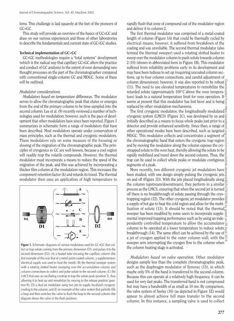
serves to allow the chromatographic peak that elutes or emergesfrom the end of the primary column to be time-sampled into thesecond column. Lee et al. (9) recently reviewed a number of tech-nologies used for modulation; however, such is the pace of devel-opment that other modulators have since been reported. Figure 1summarizes in schematic form a range of modulators that havebeen described. Most modulators operate under conservation ofmass principles, such as the thermal and cryogenic modulators.These modulators rely on some measure of the focusing orslowing of the migration of the chromatographic peak. The prin-ciples of cryogenics in GC are well-known, because a cool regionwill readily trap the volatile compounds. However, the thermalmodulator must incorporate a means to reduce the speed of themigration of the peak, and this was achieved by incorporating athicker film column at the modulation region. This increases thecomponent retention factor (k) and retards its travel. The thermalmodulator then uses an application of high temperature to

rapidly flush that zone of compound out of the modulator regionand deliver it to column 2.

The first thermal modulator was comprised of a metal-coatedlength of column (Figure 1A) that could be thermally cycled byelectrical means; however, it suffered from breakdown of thecoating and was unreliable. The second thermal modulator (alsotermed the thermal sweeper) used a rotating slotted heater tosweep over the modulator column to push solute towards column2 (10) (shown in abbreviated form in Figure 1B). This modulatorsuffered from reliability problems early in its development andmay have been tedious to set up (requiring uncoated column sec-tions, up to four column connections, and careful adjustment ofcolumn dimensions); however, it was also reported to be robust(11). The need to use elevated temperatures to remobilize theretarded solute (approximately 100°C above the oven tempera-ture) leads to a natural temperature limit for oven operation. Itseems at present that this modulator has lost favor and is beingreplaced by other modulation mechanisms.

The first cryogenic modulator, the longitudinally modulatedcryogenic system (LMCS) (Figure 1C), was developed by us andinitially described as a means to focus whole peaks just prior to adetector and provide enhanced sensitivity. Since then, a range ofother operational modes have been described, such as targetedMDGC. This modulator collects and concentrates a segment ofthe chromatographic band that enters the cryogenic trap regionand by moving the modulator along the column exposes the cry-otrapped solute to the oven heat, thereby allowing the solute to berapidly mobilized and travel down the second column. Thus, thetrap can be used to collect whole peaks or modulate contiguoussegments of a peak.

More recently, two different cryogenic jet modulators havebeen studied, with one design simply pulsing the cryogenic jetson and off (Figure 1D). With the jets placed longitudinally alongthe column (upstream/downstream), they perform in a similarprocess as the LMCS, ensuring that when the second jet is turnedoff there is no breakthrough of solute passing through the cryo-trapping region (12). The other cryogenic jet modulator providesa supply of hot gas to heat the cold region and allow for the mobi-lization of solute (13). It should be noted that the thermalsweeper has been modified by some users to incorporate supple-mental improved trapping performance such as by using an inde-pendently controlled temperature to allow the accumulatorcolumn to be operated at a lower temperature to reduce solutebreakthrough (14). The same effect can be achieved by the use ofa jet of cryogen applied to the outer column wall, with thesweeper arm interrupting the cryogen flow to the column whenthe column heating stage is activated.

Modulators based on valve operation. Other modulatordesigns sample less than the complete chromatographic peak,such as the diaphragm modulator of Synovec (15), in whichmaybe only 5% of the band is transferred to the second column.Because this can operate at a relatively high frequency, it can beused for very fast peaks. The transferred band is not compressedbut may have a bandwidth of as small as 10 ms. By comparison,the valve system of Seeley (16) (as depicted in Figure 1E) wouldappear to almost achieve full mass transfer to the secondcolumn. In this instance, a sampling valve is used to collect

Figure 1. Schematic diagrams of various modulators used for GC×GC that col-lect or trap solute coming from the primary dimension (D1) and pulses it to thesecond dimension (D2): (A) a heated tube encasing the capillary column (thefirst example of this was that of a metal paint-coated column, a supplementaryelectrical supply was used to heat the metal); (B) the thermal sweeper systemwith a rotating slotted heater sweeping over the accumulation column andcolumn connections to collect and pulse solute to the second column; (C) theLMCS that uses an oscillating cryotrap to trap the solute peak (position T), thusallowing it to heat up and remobilize by moving to the release position (posi-tion R); (D) a dual jet modulator using two jets to supply localized cryogeniccooling to the column; and (E) an example of the valve system that partially fillsa loop and then switches the valve to flush the loop to the second column (thediagram shows the valve in the flush position).

Dow


ic.oup.com/chrom



278

solute coming from the end of the primary column into a collec-tion loop, then upon switching the valve and backflushing thesampling loop into the second column at a very high flow rate,fast GC is achieved with a fast sample flux into the detector. Thekey to this method is the relative flow rates of carrier gas in eachsection (e.g., 0.75 and 15 mL/min, respectively).

It should be noted that all of these designs essentially arecapable of generating the same sort of GC×GC result with datatransformation that give sample peaks spread over a 2D separa-tion space. It may be that certain modulators will be found to havespecific benefits for selected analyses (e.g., for more volatile sam-ples or high-temperature operation), which will become moreapparent as further applications are studied.

Column considerationsPhase selection. The choice of which column phases to use in

the two-column experiment is governed by the need of whetherto achieve maximum component separation for a particularsample. This may be interpreted in terms of the columns’“orthogonality” (17), which is intended to maximize the difference in the columns’ separation mechanisms with respect to the chemical components that are to be separated. The“normal” combination for the column set appears to be a non-polar column followed by a polar (more selective) phase. Therationale for this is that the first column separates according todispersive forces (with solutes presented at the end of the firstcolumn according to their boiling points), thus coeluting compo-nents may have a wide range of polarities. The second columnthen is chosen to enhance the separation of these when they arepulsed to column 2. In the reverse geometry, a nonpolar secondcolumn may be less effective in resolving different polaritysolutes, and dispersive forces alone may be insufficient to provideeffective resolution.

It is possible to use a more selective phase in the primarycolumn, followed by the less selective. This was the case for poly-chlorinated biphenyl (PCB) analysis on a liquid-crystal-phase firstcolumn (18). It should be pointed out that it may still be a matterof trial and error in the selection of a column set, although somelogical choices can easily be made. For instance, for petroleumproducts a low polarity phase (e.g., a 5%-phenyl-polysiloxane-type column, which is often used in single-column analysis) cou-pled with a high-percent phenyl phase is a good choice. This isbecause the purpose of the separation is to achieve the resolutionof saturated compounds from coeluting unsaturated/aromaticcompounds. A high-percent phenyl phase is good for this,because π–π interactions will selectively retain aromatics on thesecond column compared with alkanes and cyclic alkanes, whichmay coelute from the primary column. Interestingly, similarlogic was used to decide on the column set for an atmosphericorganic analysis in which the aromatic content of the sample wasof interest (19).

In an attempt to predict the relative positions of fatty-acidmethyl esters in the 2D space, the use of retention indices on eachof the two columns to be used for GC×GC was modeled andapplied to the GC×GC case (20). The results were not sufficientlyaccurate to allow for confirmation that this approach could beused as a general predictor of relative elution on GC×GC; how-ever, this application may have been too subtle a problem to

reduce mathematically. Studies of essential oil analysis yield twomain observations. First, a column set that gives an enhancedseparation of oxygenated components (e.g., oxygenated mono-and sesquiterpenes) will be useful to “pull apart” these regionsand provide resolution of the complex components. ABPX5–BP20 set has been used for this task. However, for the dif-ferent hydrocarbon components (saturated and unsaturated ter-penes) it may be that this column set is not the best. This gives anextra complexity to the determination of the instrumentalrequirements for optimized separation. For chiral analysis, wehave used both the chiral column in the first dimension andsecond dimension to compare the performance of analysis forlavender. Chiral components are displayed as pairs of peaks ineither the first dimension or second dimension, respectively. As towhich is the preferred presentation, that will likely depend oninterferences in the sample.

Seeley (16) used two different phase combinations to study a range of synthetic mixtures choosing two columns that gave enhanced identification power for all components. Thecolumn set was comprised of a 10-m-long thick-film (1.4 µm) primary column of DB624 phase with 5-m-long secondarycolumns of 0.25-µm-film-thickness DB-Wax and 0.50-µm-film-thickness DB-210 phase. All columns were of the same innerdiameter (0.25 mm).

Column dimensions. The GC×GC result can only be achieved ifthe analysis on column 2 is performed “fast”. Thus, a completeelution on column 2 will be required in a few seconds. This putscertain demands on column 2, thus it will usually be a shortcolumn of narrower inner diameter and with a thin film thick-ness. It should be noted that generally column 1 is a conventionalcapillary column, but it can also equally be a shorter column thantraditionally used. Therefore, as the technique continues toevolve, new concepts in the implementation of coupled columngeometries will develop. The narrow-bore column will have amuch faster average linear carrier flow velocity (e.g., going froma 0.25-mm-i.d. to a 0.1-mm-i.d. column will result in a carrierflow increase of approximately 6-fold). This may have implica-tions on the efficiency of column 2, thus column 1 could be oper-ated at a much lower flow than normal to allow column 2 toexhibit its best performance. It is not a strict requirement thatcolumn 2 should be a narrower-bore capillary column. It shouldbe appreciated that variation in column flows through column 1will deliver solute to column 2 at different temperatures when atemperature program operation is used, thus this affects theretention on column 2. Because the relative separation of compo-nents will also be a function of temperature, the interplay ofexperimental conditions in terms of optimization will be rathercomplex. As a starting position, a 1- to 1.5-m column of 0.1-mmi.d. might be used in the second dimension, but some of our workhas also used columns as short as 30 cm. Again, this depends onthe k values and carrier flow in this dimension. Column filmthickness may be as low as 0.05–0.1 µm, and this has an impacton column activity if very polar or acidic/basic components are tobe analyzed.

The differential flow technique differs from those previouslymentioned in as much as a high flow is required through column2, thus the use of narrow columns has not been suggested and

Dow


ic.oup.com/chrom



279

similar inner dimensions for columns 1 and 2 have beenemployed.

Detector considerationsFlame ionization and electron capture. Fast data acquisition is

critical for fast GC peaks, thus with peaks having a 150-ms basewidth and smaller (peaks as narrow as a 50-ms base width havebeen reported) then 50–100 Hz data frequency is needed. A 50-Hzdetector acquisition for a 50-ms base width peak will give maybefive measurements over the peak (it should be noted that the peakis wider than the 4σ width given by the conventional base widthmeasure), which will be inadequate to draw an accurate peakshape. Ten points would be preferable, thus 100 Hz data acquisi-tion is preferred in this case.

Not surprisingly, flame ionization detection (FID) has been thedetector of choice in most GC×GC works to date. It was the firstof the regular GC detectors available for fast analysis, and today100–200 Hz operation is available in newer GCs. Some early usersof GC×GC modified their slow detectors to be compatible withfast peaks. Faster data acquisition, however, also means greaternoise levels (noise increases as the square root of the data rateincreases), because the slower rate acts as a buffer to the naturalelectronic noise fluctuations of the transducer. This affects thesensitivity enhancements that GC×GC can achieve (as will be dis-cussed).

Other ionization detectors will be generally suited for fast oper-ation if the same electronic data-handling circuitry as the FID isused. The other major requirement is that the detector trans-ducer responds in a reliable fashion to the rapid flux variation inthe detector cell. Thus, the time constant of response must becommensurate with the peak mass flux profile. The electron cap-ture detector also is now available as a fast data rate device, andthe thermionic detector should be likewise relevant to GC×GCuse. Just as packed column detectors underwent a technicalimprovement when capillary columns were developed, regularcapillary detectors must also be redesigned for very fast GC.Microcell designs with smaller internal volumes will be requiredto preserve the narrow time profiles of the GC peaks. Few appli-cations are presently available on those other than the FID, thusfurther developments in the use of different detectors areawaiting.

Mass spectrometry. There are two aspects of interest withrespect to mass spectrometry (MS) when applied to GC×GC. First,many laboratories routinely use GC–MS to provide some measureof identification for their GC analyses. Thus, there is an expecta-tion that MS should be available for GC analysis. The secondaspect is that given the considerable separation power thatGC×GC has demonstrated for complex samples, it is importantthat the separated peaks be unambiguously assigned to specificmolecular species, thus MS will validate the claims of the high-resolution nature of GC×GC and provide valuable confirmation ofits superior molecular discrimination.

The same considerations of data-acquisition speed will equallyapply to MS. Thus, the MS must present data at the rate of onemass spectrum (or one scan) every 0.02 s or better. This acquisi-tion data rate is beyond the rate that standard scanningquadrupole MSs can presently achieve, thus conventional MS is

unsuitable for GC×GC analysis. However, one report indicatedthat the GC×GC analysis could be slowed down to allow one rea-sonable scan across a peak and thus confirm peak identity (21).Such an approach is tedious and unlikely to be very practical, butit was a useful study that pointed out the demands that GC×GCplaces on the MS detection step. Time-of-flight MS (TOFMS)technology permits data acquisition at thousands of spectra persecond; these data may then be bunched to allow for presentationat up to 100 spectra/s. This is sufficiently fast for GC×GC applica-tions. Presently, only a handful of applications have used TOFMSfor GC×GC analysis, such as for petroleum products and essentialoils (22,23). These have clearly shown that TOFMS does offer toGC×GC the necessary quality of spectra to permit identificationand library-searching capabilities to support the interpretation ofthe complex 2D separation maps of GC×GC. One drawback is thatthe TOFMS suppliers do not offer data systems that supportGC×GC data presentation formats, thus data manipulation is stillvery much a manual operation. Data files are also very large(hundreds of megabytes).

There is, however, one fundamental advantage that GC×GCoffers. In many analyses of overlapping compounds, GC–MS is theonly way to obtain a unique quantitative analysis of the sample.Thus, GC–MS is necessary for the apportionment of the properamounts of each compound in the unresolved chromatogram.With GC×GC the components are now largely completely

Figure 2. A normal nonmodulated GC peak (A), in-phase modulated GC peakpulses in GC×GC (B), and 180° out-of-phase modulated GC peak pulses in

Dow


ic.oup.com/chrom



280

resolved (provided that the correct column set is used) andTOFMS is not required for the quantitative analysis of all samples,apart from the initial decision of locating and identifying com-pounds within the 2D map. Once these have been assigned, theGC×GC analysis can be used with confidence for all analyses ofthe same sample type, without requiring TOFMS.

The current interest in both GC×GC and TOFMS should pro-duce a rapid expansion in availability and use of GC×GC–TOFMSfacilities in the near future.

Modulation phase and frequencyEffect of modulation phase and frequency (conceptual framework)

Murphy et al. (24) considered the effect of sampling rate on resolution in a comprehensive two-dimensional liquid chro-matography (LC×LC) experiment. Included in the study werecomments on the effect that sampling phase had on resolution.Results were presented only as 2D plots, thus the effect that thephase had on the sequence of pulses in the second dimension wasnot clear. The nature of the study and chromatographic modesemployed did not lead to the very high resolution and sensitivityattainable in GC×GC, because zone compression effects usuallyaccompanying the GC×GC modulation process were not soreadily achieved in LC×LC. Therefore, it was instructive in thisstudy to investigate the same concepts in the GC arena. They did,however, conclude that the primary dimension peak should besampled at least three (and in some cases four) times into thesecond dimension if the resolution is not to be degraded. Also, ithas been repeated in a number of literature reports that the mod-ulation of the chromatographic signal eluting from the firstdimension in GC×GC should be of a frequency that leads to “sev-eral” slices of each peak being delivered to the second column(25). Thus, if a peak is 20 s wide at its extremities (it should benoted that this is a broader definition than the formal base widthof a peak), then use of a modulation duration of 4–5 s might beindicated. Narrower peaks will therefore either require fastermodulation or have fewer modulation events. There has beenlittle discussion in the literature as to the implication of thesechoices. In addition, not only is the number of modulationsacross each peak of concern, but also is the relative “position” ofthe modulation over the chromatographic signal. Both of theseparameters will have an effect on the presentation of the pulsedpeak profiles generated on the second column in terms of thenumber of pulses and also the shape of the pulsed peak envelope.

In the work described in this study, the relative position of themodulation events with respect to the chromatographic band isreferred to as the phase of the modulation. Figure 2 illustratestwo modulated peak profiles for modulation phases that are max-imally out-of-phase. Figure 2A is the nonmodulated peak pro-duced at the detector. Figure 2B and 2C are pulses that shouldessentially have the same envelope shape as the peak outline inFigure 2A. Although these three diagrams are drawn exactlyaligned, the cryogenic trapping process will delay the peaks’ pas-sage (by up to the duration of the trapping event time) throughthe trap, and thus the arrival time of the peak at the detector willnot exactly match that of the nonmodulated case. Therefore, thelower traces should be slightly offset to longer retention times(tRs).

Figure 2B is a trace that gives a symmetric pulse sequence witha single maximum peak. This case will hence be referred to as thein-phase case. Figure 2C is still symmetric but has two (equal)maxima; this is the 180° out-of-phase case. These will give thetallest and smallest maximum responses for the modulated peakpulses, respectively. Any intermediate modulation phase will gen-erate an asymmetrical profile, and the tallest peak will be betweenthe two limiting response maximum conditions. Each set ofpulsed peaks will have the same total peak areas (equal to that ofthe peak in Figure 2A). The absolute peak heights of Figures 2Band 2C compared with Figure 2A will depend on the frequency ofmodulation and will both be considerably taller than the peak inFigure 2A. Thus, if a modulation zone compression event is sym-metric about the peak maximum (mean) (i.e., it includes the peakmean and an equal amount of band at either side of the mean)then it will be called in-phase modulation.

The modulation process can be stepwise varied in its phasefrom being in-phase through to the 180° out-of-phase position, inwhich one compressed zone collects the part of the band imme-diately prior to the peak mean position and the next collects thepart immediately after the peak mean. It follows then thatbetween 180° and 360° the modulation events shift away fromthis out-of-phase position to eventually again be in-phase (at360°). Because each of these phase settings effectively pulses dif-ferent amounts of solute over the total chromatographic peak,the series of pulsed peaks for each phase will produce a differentdisplay of pulsed peaks (both in position and amplitude). It hasbeen long recognized that the peak maximum given in GC×GCdepends on which part of the peak is collected in the largest fluxof material. Recently, Lee et al. (26) produced a model for thisvariation in amplitude enhancement that can be achieved with anexponential relationship between the modulated secondarycolumn peak width and the amplitude enhancement proposed(26). The model confirmed the well-recognized effect that collec-tion duration will have on the peak height increase in the GC×GCexperiment. However, an experiment that demonstrates thisquantitatively during a chromatography analysis was notdescribed. In this study such an experiment will be illustrated.Described will be how the experiment may be conducted, and itwas explored how the variables may be adjusted. Peak maximaand the tR value changes that are obtained from different modu-lation phases were compared, and results illustrate that thepulsed peaks obey the cumulative distribution function for aGaussian peak. Although this should be expected, it is useful toshow this effect experimentally. In this case, the pulse period usedto modulate the peak may be represented in terms of the standarddeviation (SD) of the peak width. Finally, an example of a multi-component sample consisting of semivolatile aromatics was usedto demonstrate how the modulation duration affects the resolu-tion in a 2D presentation of GC×GC data.

The relationship between modulation timing events and peakelution time is normally “random”, thus there is usually no dis-cussion of the modulation phase and subsequent peak pulse pro-files obtained from the GC×GC experiment. Therefore, the pulsesof peaks seen in GC×GC may be anywhere from in-phase to 180°out-of-phase, and the appearance of different phases for pulsedpeaks should be recognized and accepted. By sequentially alteringthe modulation phase in successive chromatographic analyses

Dow


ic.oup.com/chrom



281

with a presentation of the series of pulsed peak profiles generatedthat demonstrate the effect of the relative modulation phase, aseries of phases from in-phase through to 180° out-of-phase casesmay be defined. The two limiting cases (in-phase and 180° out-of-phase) produce symmetric peak pulse profiles. The tR of the max-imum pulsed peak varies according to the modulation phase, andthe peak height enhancement depends both on the frequency andmodulation phase employed. Estimation of the real peak tR (peakmean) of a modulated peak can be derived from the peak pulseareas. The contour plot of a peak that is generated in two dimen-sions also depends on the frequency and phase of modulation.The slowest modulation period used in this study gave up to a30% difference in contour width (depending on the manner inwhich the peak was modulated), and this had ramifications on theapparent resolution seen in the contour plot of a complex sample.

This study that was designed to illustrate these effects will beoutlined in some detail and has not been previously reported inthe literature.

Experimental

EquipmentA Model 6890 GC (Agilent Technologies, Burwood, Australia)

fitted with an FID operated at a data-acquisition rate of 100 Hz, asplit/splitless injector operated in 1:10 split mode, and a 7683Series (Agilent Technologies) automatic liquid sampler was usedthroughout. Hydrogen was employed as the carrier gas and oper-ated in the constant flow mode. ChemStation event control(Agilent) was used to instruct the modulation control system tocommence modulation at a precise time, and the ChemStationdata system (Agilent) was used to record the detector output. Itshould be noted that in this study, it was important that the mod-ulator timing be very precise (i.e., the modulation events be con-trollable to better than 0.1 s, for example) and in particular thatthe commencement time of the modulator be accurate. In thesystem used in this study, the run-to-run reproducibilityexceeded that required, thus allowing the effect of the modulationphase to be studied.

The cryogenic modulator employed for the GC×GC experimentwas the LMCS Everest Model (Chromatography Concepts,Doncaster, Australia), which was retro-fitted to the 6890 GC. CO2maintained the temperature of the modulation trap to at least100°C below the prevailing oven temperature. The operation anddemonstration of the principles of this system can be obtainedelsewhere (27,28).

Column sets and experimental procedureA dual-column arrangement comprised of a primary column of

25-m × 0.22-mm i.d. with a 1.0-µm film thickness (BPX5-coatedcolumn, 5% phenyl-dimethyl siloxane phase, nonpolar) directlyconnected to a short second column of 1.2-m × 0.1-mm i.d. witha 0.1-µm film thickness (BPX50-coated column, 50% phenyl-equivalent polysilphenylene phase, polar) was used for all studies.Both columns used were manufactured by SGE International(Ringwood, Australia).

The cryogenic trapping system was operated under selectedmodulation timing periods (or durations) of 2, 3, 4, 6, 8, or 9.9 s (as

indicated in the respective phases of this study) and a hold time of0.5 s in the release position. For studies using linalyl acetate, themodulator start time was at least 1 min prior to the expected solutetR (i.e., approximately 16 min). In some studies the start time wassequentially incremented by 0.01 min in order to alter the modu-lation phase of the cryotrap with respect to the peak elution. Byappropriate calculation it was possible to estimate a start time thatwill give an in-phase modulation, and from this start time themodulation phase was then varied in 0.01-min intervals until thecycle was completed (i.e., through 180° out-of-phase to 360° in-phase). The GC oven was operated under a temperature programrate of 60°C (held for 1 min) heated to 120°C at 20°C/min, then to150°C at 2°C/min, and finally to 180°C at 20°C/min. This temper-ature program was used to give a suitable peak width such that arange of modulation frequencies could be used to study the effectof this variable (i.e., giving a number of pulsed peaks for the inter-mediate frequency chosen) and permit a number of modulationstart times incremented by 0.01 min to be used.

Modulation timing periods of 2, 3, 4, 6, 8, and 9.9 s were usedfor the semivolatile aromatics. The modulation start time waskept constant while the modulation timing periods were varied.The semivolatile aromatic mixture was analyzed using a temper-ature program of 40°C (held for 1 min) heated to 150°C at20°C/min and then to 230°C at 2°C/min. A split ratio of 40:1 wasemployed.

SamplesLinalyl acetate was provided by Australian Botanical Products

(Hallam, Australia), and the semivolatile aromatic sample was from

Figure 3. Correlation of phase of modulation and peak elution. A delay of 0.03min results in a 180° out-of-phase modulation case with the 0.03-min delayexactly midway between pulses 1 and 2 in the original modulation (dottedline), and a 0.06-min delay gives a result that is in-phase with the original mod-ulation (dashed line). The vertical line shows that the central zone of the peakis exactly captured in the third modulation and thus this will give an in-phaseresult equivalent to Figure 2B.

Dow


ic.oup.com/chrom



282

Ultra Scientific (Kingston, RI) (part number SVM-124-1). Linalylacetate was diluted with hexane in order to prevent overloading ofthe peaks when the GC×GC experiment is conducted. The samelinalyl acetate solution was used throughout this study apart fromthat used for experiments for the reproducibility of retentions andthe studies of modulation timing periods of 3 and 4 s.

Results and Discussion

Correlation of modulation phase with peak elutionIn order to demonstrate how the two different results (Figure

2B and 2C) and the intermediate pulse profiles were generated,Figure 3 presents a pulse train that shows the positions of thecryomodulator and the relative event times for the commence-

ment of the modulation of the cryotrap that may be used. The ver-tical rectangular pulses represent when the trap moves to theelute position. A hold time of 0.5 s was imposed, and the returnmovement to the home trapping position occurred when therectangular pulse returned to the baseline. Figure 3 shows that insuccessive GC analyses, the trap was delayed in the modulationstart time by 0.01 min. With a delay of 0.03 min, the peak pulseswere still out-of-phase (by 180°) with the original sequence. Inorder to reach a modulation sequence exactly in-phase with thatused initially, the delay would need to be 0.06 min = 3.6 s, thus themodulator was operated at a pulse duration of 3.6 s for thisexample.

If a migrating peak entered the cryomodulator such that itscentral zone was fully collected in one trapping event (i.e., thetrap event was symmetrical about the peak maximum), then asymmetric peak profile of the type in Figure 2B was obtained. Itshould be noted that there is no control over this situation in anormal GC analysis, and among the pulsed GC×GC peaks it maybe that none of them give an exact symmetrical set of peak pulses.

In Figure 3, the modulation timing can be adjusted to give arange of phases between 0° and 180° (i.e., fully out-of-phase) andup to 360° (in-phase with 0°). In order to present sufficient com-parative profiles over a full 360° phase change, a variation in thecommencement of successive GC experiments of 0.01 min waschosen. Thus, for a 3.6-s modulation period (0.06 min = 360°),there were six successive GC analyses before the modulatorrepeated the original pulsing phase pattern (60° for successiveexperiments).

Reproducibility of retentionsIn order to appropriately study the effect of the modulation

phase experimentally, it is a requirement that the run-to-runreproducibility of peak retentions is better than the time variationof the modulation experiments (e.g., 0.01 min above). This willensure that the comparison of peak profiles in successive experi-ments will be meaningful. The 0.01-min interval in the modula-tion start times was 0.6 s. The peak retention reproducibilityshould be much better (i.e., smaller) than this. Table I lists datafor peak retention in 11 repeat nonmodulated experiment anal-yses. The SD of peak tR was 0.002 min (or 0.12 s), thus this was 5

times smaller than the time variation of the mod-ulation phase and should be suitable for the studyas proposed. The first entry in Table I (6.427 min)may be rejected as an outlier, which gives muchbetter tR reproducibility. Peak areas and heightseach had a relative SD (RSD) of 0.8%.

The modulator reproducibility was thenchecked by successive injections of the samesample. A pulse duration of 3 s (0.05 min) wasused. Table II lists these data. The SD and RSDvalues for most of the retentions were so small asto be negligible (e.g., RSD of 0.006% or less). Theimproved peak time reproducibility comparedwith that in Table I arose from the very preciserelease time of the modulator and the shortcolumn length, thus a small tR interval on thissection of the column between the modulator anddetector. Carrier gas flow precision will also be

Table I. Reproducibility of Peak Retentions in Normal GCMode

Run no. tR (min) Peak area (pA•s) Peak height (pA)

1 6.427 73.781 23.8582 6.431 74.164 24.2143 6.432 73.784 24.2604 6.432 75.190 24.2315 6.433 74.902 24.2046 6.432 74.880 24.2907 6.431 74.540 23.8638 6.432 74.538 24.0929 6.433 75.164 24.031

10 6.432 75.086 24.24811 6.433 75.447 24.496Average* 6.432 74.680 24.162SD* 0.002 0.570 0.189%RSD* 0.026 0.764 0.783Average† 6.432 74.769 24.193SD† 0.001 0.513 0.169%RSD† 0.011 0.686 0.697

* All data.† Rejecting Run #1 data.

Table II. Reproducibility of Peak Retentions in the GC×GC Mode*

tR for peak ∆tR values between Chromatogram pulse no. (min) peak pulses (min)from Figure 3 1 2 3 4 2-1 3-2 4-3

A 17.052 17.102 17.151 17.201 0.050 0.049 0.05B 17.052 17.102 17.151 17.201 0.050 0.049 0.05C 17.052 17.103 17.153 17.201 0.051 0.05 0.049D 17.052 17.102 17.152 17.201 0.050 0.05 0.049E 17.052 17.103 17.153 17.201 0.051 0.05 0.048Average 17.052 17.1024 17.152 17.201 0.0504 0.0496 0.0492SD 2.4 × 10–7 0.00055 0.0010 3.4 × 10–7 0.00055 0.00055 0.00084%RSD 1.4 × 10–6 3.2 × 10–3 5.8 × 10–3 2.0 × 10–6 1.1 1.1 1.7

* A 3-s modulation duration was used giving ∆tR values close to 0.050 min for successive pulses.

Dow


ic.oup.com/chrom



283

critical. This appeared to be excellent.Although tR values are very precise, the peak areas and heights

of the pulsed peak profile are less precise. Table III reports thesedata. The first analysis may be rejected, and the resultant improvedreproducibility can be seen in Table III. Considering these latterdata, it is apparent that the profile was well-reproduced. It was pre-sumed that the small variations in Table III were a result of slightpeak retention differences when the peak enters the cryotrap,which means that the mass flux of solute into the cryotrap in agiven peak pulsing period varied slightly. Total peak area repro-ducibility was good. The first entry again appeared to be an outlier,although there did not seem to be a reason for this. Deleting thisrow of data gives improved reproducibility (as shown in Table III).Figure 4 illustrates the five GC traces for this data, and the anoma-lous first run is apparent. It can be concluded that the GC andmodulator performance were suitable for the proposed study.

Table III. Reproducibility of Absolute Peak Pulse Areasfor a 3-s Modulation with the Largest Four Pulsed PeaksReported

Chromatogram Peak areas for peak no. Total from Figure 4 1 2 3 4 peak area

A 20.45 113.78 122.04 25.04 281.32B 10.22 83.74 141.57 43.7 279.24C 8.79 77.71 143.54 49.29 279.33D 6.66 69.52 142.27 53.59 272.03E 7.7 73.34 142.85 52.26 276.15Average* 10.76 83.62 138.45 44.78 277.61SD* 5.57 17.67 9.20 11.67 3.63%RSD* 51.78 21.13 6.65 26.06 1.31Average† 8.34 76.08 142.56 49.71 276.69SD† 1.52 6.11 0.84 4.39 3.44%RSD† 18.27 8.03 0.59 8.83 1.24

* All data.† Rejecting data of Figure 4A.

Figure 5. Variation in the phase of modulation for a 3-s modulation duration(conditions are the same as in Figure 4). The modulation phase was altered bysuccessively delaying the start time by 0.01 min from A to F, with an initial starttime of 16.00 min. A and F approximate the same modulation phase, thus pro-duce almost equivalent results. The time shift in the maximum peak can bereadily seen in this series of analyses. Table IV presents the pulsed peak timesand areas for the chromatograms in this figure.

Figure 4. Reproducibility of peak pulses generated using a 3-s modulationduration for linalyl acetate (conditions found in the Experimental section) insuccessive chromatographic analyses. The chromatogram in A is an anoma-lous result (as seen in Table III). The profiles for the chromatograms in B throughE are very reproducible.

Dow


ic.oup.com/chrom



284

Variation in modulation commencement timeBy varying the start time of the modulator for a series of GC

analyses and with the peak tR unchanging, it is possible to have acontrolled variation in the phase of the pulsing of zones of themigrating peak. Figure 5 illustrates this behavior. Because a mod-ulation duration of 3 s was used and the modulation start timewas incremented in steps of 0.01 min, after 5 increments thesame modulation phase was repeated. Thus, it can be seen thatFigure 5A should be reproduced in Figure 5F. This was approxi-mately the case. It should be noted that the profile pattern ofpeaks moved to the right in steps of 0.01 min, and as this shiftoccurred with the input peak position to the cryomodulatorunchanged, there started to appear an earlier peak while the latestpeak appeared to diminish. The largest peak in Figure 5A at 46.7%of the total area progressively decreased to 32.7% in Figure 5F (asthe zone that was compressed in the cryotrapping process pro-gressively decreased because this modulation event movedtowards the trailing end of the peak) when it had the same time asthe fourth peak of Figure 5A with an area percentage value of27.8%. The second peak in Figure 5A steadily increased from19.3% to 44.0% in Figure 5F when it had the same time as thelargest peak in Figure 5A (which had an area percentage value of46.7%). Table IV lists the data for the respective peaks in thesetraces. The time of peak 1 was 17.104 min for Figure 5A andincreased sequentially by 0.010 min up to 17.135 min for Figure5D. In Figure 5E, a new first peak appeared because of the phaseshift of the modulation (thus it had a time of 17.094), and finallyin Figure 5F the modulation was 360° out-of-phase from that ofFigure 5A, which means it became in-phase (thus the first peakagain had a time of 17.104 min). The tallest peak in the tracesvaried from an area percentage of 47.7% (Figure 5B) to 39.9%(Figure 5E), which was a change of approximately 16%. Thisoccurred as the peak profile changed from a symmetric distribu-tion (represented by Figure 2B) to a symmetric distribution (rep-resented by Figure 2C). These two experiments varied by 0.03min, which was close to the 180° out-of-phase value of 0.025 min(it should be noted that there was no pair of figures that had anexact 180° difference because the modulation time was varied by0.01 min in each step). The total peak areas varied from 1038 to1185 pA•s, but this generally will reflect sample delivery effi-ciency and should not alter the peak area percentage values.

Figure 6 and Table V report the same study as described previ-

ously, except with a modulation duration of 6 s (double that usedpreviously). The modulation start time was again varied by 0.01min. The figures presented were every second in the series, thusthey were 0.02 min apart. Figure 6C approximates one of the sym-metric profiles and Figure 6F approximates the other. It should benoted that the largest peak in Figure 6F had an area percentage of81%, whereas it was 49.5% in Figure 6C. This equates to an areadifference between maximum peaks of approximately 39%. Thelarge variability was of course a result of the large amount of peakthat was zone compressed in the case of Figure 6F (Figure 6C wasdesignated for a modulation event almost exactly at the peak max-imum), and this effectively shared the bulk of the peak equallybetween the two-zone compression events. The larger the pulseperiod, the greater is the anticipated variation in the peak maximafor the in-phase and out-of-phase cases (as can be seen by com-paring Tables IV and V).

Modulation frequency variation correlationsIt is commonly accepted that approximately 4 or 5 pulsing

events are preferred for a solute in GC×GC; however, the actualnumber pertaining to a given analysis is often not given, nor hasthe choice of frequency been reported in terms of how the datacompare. The greater the number of modulations over a peak, theless is the sensitivity enhancement that is realized in the GC×GCexperiment over normal GC. Also, from the previous section, thepresentation of peak pulses will also vary considerably for dif-ferent modulation periods employed. It is beneficial to investigatethe variation of frequency over the peak elution and observe howthis alters the peak contours in the 2D plots that are used for datapresentation in GC×GC.

If a set modulation start time is used for a series of differentmodulation durations, then the pulsed peak profile will also varyaccording to the phase of modulation across the peak. Thus, onemodulation setting may give a symmetric pulsed peak profile andanother might be significantly asymmetric. If the experiment isconducted using a range of different start times for each of themodulation frequencies to be used, then it will be possible to selectfrom the whole data set a series of pulsed profiles of similar mod-ulation phase (e.g., in which all give symmetric distributions).

Both of these cases will be instructive in the interpretation ofthe results. It should be noted that it would be possible to com-pute which frequencies should give which pulsed peak profiles

Table IV. tRs, Peak Relative Areas, and Total Peak Area for a Series of Phase Increment Analyses in 0.01-min Steps Using a 3-s Modulation Duration*

Figure 5A Figure 5B Figure 5C Figure 5D Figure 5E Figure 5FTime (min) %Area Time (min) %Area Time (min) %Area Time (min) %Area Time (min) %Area Time (min) %Area

Peak 1 17.104 2.2 17.114 3.0 17.125 4.4 17.135 6.4 17.094 0.8 17.104 1.6Peak 2 17.155 19.3 17.165 22.1 17.176 26.8 17.186 31.1 17.145 11.1 17.155 15.8Peak 3 17.206 46.7 17.216 47.7 17.226 47.7 17.236 46.4 17.196 38.9 17.206 44.0Peak 4 17.255 27.8 17.265 23.9 17.275 18.6 17.285 14.4 17.246 39.9 17.256 32.6Peak 5 17.304 4.1 17.314 3.3 17.324 2.4 17.335 1.8 17.294 8.2 17.304 5.2Peak 6 17.345 1.1 17.355 0.8Total peak area 1039 1095 1111 1101 1162 1186

* Two analyses gave six peak pulses.

Dow


ic.oup.com/chrom



285

by estimation of the modulation phase during peak elution.Figure 7 presents data for a series of modulation frequencies (2-,

3-, 4-, 6-, and 9.9-s period) for the same start time (16.03 min).Figure 7A (2 s duration) gives approximately 7 pulses across thepeak. The maximum pulsed peak was at approximately 17.14 min.A 4-s pulse modulation gave only 3 peak pulses (the maximumbeing at approximately 17.12 min). Three pulses were also seen fora 6-s period (maximum pulse at 17.175 min) and the 9.9-s modu-lation (2 peaks) (maximum pulse at 17.225 min). The maximumpeak among the pulsed sets clearly shifted in its tR value, and thelatest possible maximum peak elution was where the slowestmodulation (9.9 s in this case) commenced in collecting themigrating solute just prior to the peak maximum flux enteringthe trapping zone. In this case the tR value of the latest possiblepeak was equal to approximately the sum of the time that the cry-otrap started collecting the solute plus the tR on the secondcolumn plus the modulation time. Thus, it could potentially be upto 9.9 s longer than that of the peak maximum obtained on thesame column set at the same conditions, except that the cryofluidwas not turned on.

The trend in the heights of the maximum peak in each of thechromatograms should be noted. Because the injected quantitymay vary, the comparison was made more valid by correcting forthis by dividing the recorded peak height by the total area. TableVI shows these values. It should be noted that this interpretationis only a broad trend because it has been shown previously thatthe peak height of maximum peaks depends on the phase of mod-ulation. The data confirm that the peak height increased withdecreased modulation frequency (in this experiment by approxi-mately 230%). A similar result was found for a start time of 16.05min, and only the comparison of a 3-, 6-, 8-, and 9.9-s pulse dura-tion is shown in Figure 8. The difference shown for 8 and 9.9 s wasstriking in terms of the tR of the maximum peak pulse being17.155 and 17.225 min, respectively (i.e., 0.07 min = 4.2 s dif-ferent). This arose simply because of the relative phases of themodulation in each case.

It is possible to predict the true peak maximum for these resultsby having accurate and precise values for the peak responses,because the cumulative peak area for a Gaussian distribution is well-known, thus allowing for the calculation of exactly atwhich point in the Gaussian peak the modulation event occurs(provided that the peak SD entering the cryotrap is known in time units). Thus, it can be determined by how many units of SDthe peak pulse varies from the peak maximum. Then, using this peak’s tR and subtracting or adding the number of SDs timesthe SD value, the true peak maximum will be estimated. The

Figure 6. Variation in the phase of modulation for a 6-s modulation duration(conditions are the same as in Figure 4). The number of experiments for a com-plete 360° cycle was double that for the 3-s duration shown in Figure 5, butonly every second result in the series was shown (it should be noted that thepulse peak tR offset was 0.02 min, compared with 0.01 min in Figure 5).Because the modulation duration was twice that of Figure 4, there were fewerpulses across the peak, but again the result in A is almost reproduced in F,because they had relative phases approximately 360° apart.

Table V. tR Values, Peak Relative Areas, and Total Peak Area for a Series of Phase Incremented Analyses in 0.02-min StepsUsing a 6-s Modulation Duration*

Figure 6A Figure 6B Figure 6C Figure 6D Figure 6E Figure 6FTime (min) %Area Time (min) %Area Time (min) %Area Time (min) %Area Time (min) %Area Time (min) %Area

Peak 1 17.074 17.81 17.095 28.12 17.113 49.48 17.033 1.70 17.051 4.14 17.073 10.09Peak 2 17.175 78.14 17.194 69.21 17.212 48.90 17.132 71.87 17.152 80.61 17.173 81.30Peak 3 17.274 4.05 17.294 2.67 17.313 1.61 17.233 25.19 17.253 15.25 17.274 8.61Peak 4 17.334 1.24Total peak area 167.9 169.7 173.7 175.1 175.19 177.4

* Most analyses gave three peak pulses (one gave four peak pulses).

Dow


ic.oup.com/chrom



286

result for a 2-s modulation with 6 peak pulses obtained was considered (see Figure 7A). Their percentage areas were found to be 1.84%, 11.52%, 28.04%, 36.42%, 17.7%, and 4.48%. Incumulative areas, these were 0.0184, 0.1336, 0.414, 0.7782,0.9552, and 1.000, respectively. Standard tables (29) gave SDvalues for these cumulative areas (with respect to the mean value)of –2.09, –1.11, –0.217, 0.766, and 1.697, respectively (with no derived value for 1.000). This computes to be 0.98, 0.893,0.983, and 0.931 SD unit differences, respectively, between eachof these pulses. Therefore, the reproducible regular modulationprocess leads to respective peak areas of the pulses in agreementwith that predicted for a Gaussian curve, and the real peak maximum time can be derived from the times of these pulses.This is an interesting observation but probably not of too muchconcern for routine GC×GC analysis. It may, however, aid 2D peakcoordinate derivation and presentation if required in a computer-ized 2D data report.

Presentation of data in 2D contour plotsAt a longer modulation duration, some of the solutes showed

barely more than one pulsed peak compared with the multiplepeaks when a faster modulation was used. Contour plots of thesecan be used to show how the plotting package constructs the con-tours for each case. Also, it is instructive to observe the differencethat changing the modulator start time causes when generatingthe 2D contour plots. In this case, the 0.01-min delay in startingthe modulator was independent of the data-processing step(which took t = 0 as the commencement of the data stream), andthe modulation time was used to construct the data matrix.Shown in Figure 9 is the contour plots for the sequence of peaks

Figure 7. Variation in the frequency of modulation for a constant modulationstart time of 16.03 min. The modulation duration was 2, 3, 4, 6, and 9.9 s for Athrough E, respectively. Other conditions of analysis are the same as in Figure 4.

Table VI. Effect of Modulation Period on the Height ofthe Maximum Pulsed Peak with a Modulation Start Timeof 16.03 min*

Modulation Height of Total peak Normalized duration (s) maximum peak (pA) area (pA•s) height

2 1100 260 4.233 900 148 6.084 1400 181 7.746 1460 168 8.709.9 2000 203 9.85

* See Figure 7.

Figure 8. Variation in the frequency of modulation for a constant modulation starttime of 16.05 min. The modulation duration was 3, 6, 8, and 9.9 s for A throughD, respectively. Other conditions of analysis are the same as in Figure 4.

Dow


ic.oup.com/chrom



287

given in Figure 5. It should be noted that the contours shifted ver-tically by 0.01 min in the 2tR time because they were progressivelydelayed by 0.01 min in successive chromatograms, and the dataconversion was not corrected for this. This has an interestingconsequence in general GC×GC 2D plot presentation. If the starttime is not precise and the modulation phase varies from run-to-run, the 2D coordinates of peaks will not be well-reproduced. Thiswill potentially make solute identification based on peak positionin the 2D space difficult. In this study, excellent positional repro-

ducibility was seen (except for those places in which the starttimes were deliberately adjusted to alter the phase of modula-tion).

Peak 5E in Figure 9 was the contour from the pulsed peaks inFigure 5E, and it was plotted at an apparent earlier 1tR time com-pared with the other contours because its peak pulse distributionwas more skewed to a lower 1tR time. All others were not signifi-cantly different, but the excellent correspondence of 5A and 5Fshould be noted, which were the two in-phase experiments. Thecontour plots of a 9.9-s modulation rate were almost trivial(Figure 10), because there was at best only two significant peaks.They gave contours of width at 0.26 min and 0.38 min for Figure10A and Figure 10B, respectively, which corresponded with onepredominant peak and two equal peaks in the pulsed trace,respectively. In contrast, the 3-s modulation gave a 1tR contourpeak plot of width at 0.17 min. We have previously noted the effectof the contour line response in influencing the apparent size ofthe contour plot (30); in this case a similar contour level waschosen to keep this as consistent as possible. Thus, the effect ofthe modulation period on contour presentation must be lookedupon in a similar way to the effect of overloading and consequentpeak broadening in GC×GC analysis (30).

Semivolatile aromatics studyBecause in a study such as this with randomly located peak

retentions (at least with respect to the modulation phase) a studyof variation of phase by altering the start time of modulationappears to be of less utility, it would appear to be relatively easy toimplement. However, it has been shown previously that modula-tion duration strongly influences the apparent contour plot peakmagnitudes (widths in the first dimension) of the data when pre-sented in the 2D manner.

Thus, this same multicomponent semivolatile aromatic samplethat has been reported elsewhere (31) has been chosen for thisstudy. Because under the conditions chosen the solutes will havea given 2tR, when a larger modulation period is selected, thesolutes will appear bunched along a narrow elution zone (as seenfor Figure 11C at the 9.9-s modulation). In this case, the 2tR scalewas 9.9-s broad, thus it appears on the 2D space to contract theapparent elution zone. Of course, this range was constant for allmodulations, but it only looked wider as the modulation perioddecreased (i.e., the scale of the 2tR axis decreased). From Figure11C, it can be predicted that the solutes have retentions ofapproximately 2.5–5.0 s on the second column.

Figure 11A shows a 2-s modulation. From previous considera-tions, this should give the best (smallest) apparent peak contourplots at a given response level (e.g., 50 pA), and peaks fromapproximately 60–150 ms width in the second dimension werefound. These should also be the most resolved in the first dimen-sion on the plot, having a minimum contour width. By contrast,Figure 11C (9.9 s) shows the effect of longer modulation periods.The peaks marked X (which were well-resolved in Figure 11A)were plotted with a significant merging of their contours. Forcomparison, Figure 11B was a 3-s period result. Figure 12A is apresentation of an expansion of the peaks marked X (data for the9.9-s modulation) (Figure 11C), and the pulsed peak result is alsoshown. Interestingly, even though the pulsed peak result did notclearly show separate pulsed peaks for both components, the con-

Figure 10. Expanded contour plots for a 9.9-s modulation duration with a dif-ferent modulation phase. The phase difference was 0.11 min between the twochromatograms (start time for A was 15.98 min and for B was 16.09 min). Thepulsed peak profile gave essentially one peak for A and two equal peaks for B.

Figure 9. Contour plots for the chromatograms shown in Figures 5A–5F for a 3-s modulation duration. Because these were for different modulation phasesachieved by altering the start time of modulation and the data conversion ineach instance was not altered to take into account this difference, then the con-tours were offset successively by 0.01 min (0.6 s) in the second dimension. 5Aand 5F are in-phase, thus they plot at precisely the same position.

Dow


ic.oup.com/chrom



288

tour plot of Figure 12A did show two maxima in the contour. Forthe 2-s case, the pulsed presentation (Figure 12B) showed twoseries of pulsed peaks, with an apparent slight resolution for theevent in which both compounds were present in the one zonecompression step (at approximately 17.69 min). The resolutionwas quite acceptable in the contour mode. This was in accordwith the observation by Murphy et al. (24) that the higher sam-pling rate gives better resolution. The reason for the double max-imum in the first contour peak is not clear. It should also be notedthat the two compounds exhibited close to 180° out-of-phase(first component) and in-phase (second component) distributionsfor their modulated peak pulses, respectively. The peaks marked Yin Figure 11 were well-resolved in the second dimension. Figure13 shows the two pulsed peak plots for the two components at Yfor 2-, 3-, 6-, and 9.9-s modulation periods. The respective peakswere marked 16 and 17 on these diagrams. Expanded contour

plots did not need to be presented. All of the examples gave thesame retention difference and resolution between components 16and 17 in the second dimension (as seen in the resolution of 16and 17 in all of the chromatograms in Figure 13). The differencein the presentation of the pulsed peak chromatograms arisingfrom the choice of frequency was striking.

This discussion on the frequency and modulation period israther complex, although it is not easily reduced to simpledescription. The terms sound more spectroscopic than chro-matographic; however, the different presentation modes forGC×GC should be appreciated and understood by users of thistechnology as well as the reasons for the generation of differentpeak pulse patterns. Although the modulation phase affects theresolution, it is not possible to adjust the phase of modulation foreach solute in order to artificially select the most appropriatephase (i.e., in-phase modulation) because once the pulse period isset and the start of modulation commences, there is no userintervention to adjust the phase (the modulation phase is arandom event for any peak).

Figure 11. Contour plots for the semivolatile aromatic sample analyzed usingdifferent modulation frequencies. A, B, and C correspond with modulationdurations of 2, 3, and 9.9 s, respectively. Pairs of peaks with similar first-dimen-sion tR values are identified by X and Y, with X being poorly resolved on thesecond column and Y being very well-resolved on the second dimension. Forexpanded contour and pulsed peak presentations, refer to Figures 12 and 13.

Figure 12. Pulsed peak chromatograms and contour plots for peaks marked Xin Figure 11: (A) modulation phase of 9.9 s and (B) modulation phase of 2 s.

Dow


ic.oup.com/chrom



289

Sensitivity enhancement in GC×GCAny of the modulation methods that yield a zone compression

effect (such as the mass flow rate of solute into the detectorincreases) will be capable of increasing the response sensitivity ofthe analysis. It should be noted that we have already decided thatincreased data frequency does increase noise, thus there is atrade-off between a mass flux increase and the data sampling rate.However, there is a real net advantage in signal-to-noise inGC×GC.

It is often stated that an increased signal response of 20 to 50times is obtained in GC×GC compared with the normal capillaryGC experiment. The actual increase in mass flux depends on thepeak width in the normal GC analysis, the peak width at the endof the second column in the GC×GC experiment, and the fre-quency of the modulation. For a response height increase (of themaximum peak pulse), the phase of modulation should also beconsidered. A number of these factors have been described in theprevious section. A peak that is 8 s wide in normal analysis and150 ms wide in GC×GC will be potentially 50 times taller. This isthen moderated by frequency and phase considerations. In a sys-tematic study of sterols by using normal, comprehensive, and tar-geted GC, the increases in detection limits were reported to beapproximately 10 times and 40 times better, respectively, for the

latter two methods. The targeted mode fully collected each of thesterol peaks and thus had the best signal enhancement. Lee et al.(26) presented a theoretical study that showed potential improve-ments in GC×GC analysis (26).

It should be noted that sensitivity enhancement is merely withrespect to peak response height. There is no improvement in peakareas, because the injected quantity of sample is only dependenton the injection mode. However, the time compression effect doesmean that the narrow peaks now have a response that gives a sig-nificant signal above the noise level, thus a peak that might nothave been seen in conventional GC is now measurable in GC×GC.It is probably recognized that one of the major goals of chro-matography over the years has been improved sensitivity, and thisis a significant additional (but probably secondary) outcome ofGC×GC. It still may be critical in some instances.

Peak capacity increasesIf we ask ourselves why there are considerable efforts by a

number of research groups put into GC×GC there can be only oneanswer, and that is the continuing search for greater analyticalseparation power (apart from the fascinating GC results that areobtained). This is translated into a greater peak capacity over thatachieved in single-column analysis. Giddings (7) reported that acomprehensive 2D analysis should be able to produce a total peakcapacity equal to that of the product of the capacity of eachdimension. Therefore, in a two-column experiment using tem-perature programming over a period of 60 min, if the first columngenerates peaks of an average base width of 10 s (in which thisconstitutes resolved peaks), then this dimension has a totalcapacity of 600 resolvable peaks. If the second orthogonal columnis capable of separating 12 peaks in 3 s (i.e., the average peak basewidth is 250 ms), then the total available separation space has apeak capacity of 600 × 12 = 7200 peaks (i.e., it is potentiallycapable of resolving 7200 separate peaks). There is a naturalredundancy in as much as some peaks that coelute on the firstcolumn may have an insufficient polarity difference to be resolvedin the second column, but the purpose of this calculation is todemonstrate that in sheer separation power there is almost anunimaginable opportunity to study complex samples. The onlyquestion is the proper choice of column sets to ensure orthogo-nality. On a purely statistical basis, the extra peak capacity can bedirectly translated into a greater separation of components. Thishas been shown time and again in GC×GC applications and hasbeen considered theoretically by Davis (5). Seeley (16) discussedthis for a synthetic sample of 100 or more volatile compounds.

Sample analysis by using GC×GCEffect of sample amount

The role of GC×GC in the analysis of complex samples (i.e.,those with a plethora of components) naturally implies that manywill be at low levels and others will be major components. Thus,there is a wide diversity of concentration in the one sample. Asmore components are to be measured, it is increasingly impor-tant to have a wider dynamic range of analysis. In GC×GC, if weuse a second column of thin film dimensions, there is a questionof overloading the column and a subsequent peak broadening ofthe peak pulses on that column, as described recently (30). Thisreduces resolution for some instances in which primary column

Figure 13. Pulsed peak chromatograms for peaks marked Y in Figure 11. A, B,C, and D are for modulation phases of 2, 3, 6, and 9.9 s, respectively. Peak 16is the component that elutes earlier than peak 17 in both the first and seconddimensions.

Dow


ic.oup.com/chrom



290

overlapping peaks are pulsed to the second column and one ofthese is in much larger quantity. Thus, if a sufficient sample isintroduced to the column to enable the analysis of trace con-stituents, the probability of major component overload isincreased. One additional consideration is that compounds aredelivered to the second column only once they elute from the pri-mary column, and this will generally be at a temperature at whichthe component has a relatively low k value (i.e., at a temperatureat which it has a reasonably high vapor pressure), which reducesits tendency towards mobile phase overloading. This will help tomaintain a constant distribution constant (K) value with differenttotal amounts of sample injected. The role that stationary phasechemistry plays on nonlinear conditions should also be consid-ered. The tendency of compounds to exhibit convex or concaveisotherms typical of stationary phase and mobile phase over-loading defines the type of peak shape exhibited by the overloadedcomponent. Maximum peak capacity will be ensured only if linearchromatography conditions are observed. The 2D experiment,however, should mean that for certain analyses it is possible toaccept a greater degree of overloading than can be tolerated insingle-column analysis in some cases.

Analysis of complex samplesIt is not the purpose of this review to present an exhaustive

account of applications of GC×GC. With the degree of activity inthis area it is likely that new applications applying the benefits ofGC×GC for a better advantage will continually be introduced. Inorder to complete the discussion of fundamental concepts, it is nec-essary to present a selected demonstration of the technology (referto the reviews by Bertsch (32) and Marriott (33) and the discussionsin these works for further specific applications of typical separa-tions). The traditional petrochemical analysis by GC×GC is typifiedby the work of Beens et al. (34) and Frysinger and Gaines (14).

In our experience, the following sequence represents a possibleprotocol to use when approaching sample analysis. (a) Chro-matograph the sample on a column set to define the total analysistime under normal conditions (i.e., without the cryomodulationprocess). It should be noted that this column set will be any thatis currently used in one of the GCs in the laboratory, and usualsets are comprised of BPX5/BP20 or BPX5/BP50 columns. Basedon the (likely) components and logical choice of columns, eitherof these sets may be preferred as an initial choice. (b) Repeat theanalysis but now with the cryomodulator operating during theregion of interest. (c) Study the result especially with regard tothe degree of resolution of components that are pulsed to thesecond column. (d) If the resolution is insufficient, adjust theexperimental conditions to try to achieve better component reso-lution. Failing that, consider the likely effect of second-columnlength on the resolution. If this does not give the desired resolu-tion, consider a change of second-column phase or a differentcolumn set. (e) For some analytical studies, there may be a muchmore logical stationary phase combination required, rather thanthose two sets indicated previously. For instance, columns forchiral analysis may be required for enantiomer resolution, or aliquid crystal phase may be better for PCB analysis.

Figure 11 is a representative case of high-resolution 2D GC×GCanalysis of a typical sample of semivolatile aromatics. Maximizingthe use of the 2D space is the main goal for ensuring the greatest

possible number of resolved components in the analysis. It islikely that as more classes of chemical compounds are studiedand the effects of the column sets chosen for GC×GC are quanti-tated, a better use of the available space will be reduced to a morelogical process. It is also likely that the enhanced peak capacitywill benefit sample pretreatment aspects of the method protocolbecause more impurities can be accommodated within the 2Dspace without compromising the analysis of the target analytes.This should mean that the number of sample-handling stepsshould be reduced and recovery improved.

It should be noted that other chromatographic dimensionsmay be coupled comprehensively, as discussed in a reasonablythorough review by Liu and Lee (35), and this potentially extendscomprehensive separations to a wider range of solutes.

Conclusion

This review has sought to present fundamental considerationsin the GC×GC technique, its implementation, and supportingtechnologies that are specific to GC×GC. There will be a newthought process required on the part of the chromatographerwith respect to interpreting GC×GC results, and especially theneed to think in two dimensions.

This study has also reported details of experimental correla-tions of pulsing duration and the modulation phase with pulsedpeak presentation in GC×GC. The phase of the modulation, withrespect to the input distribution of a solute entering the modu-lating cryogenic trap, alters the pulsed peak presentation of data,particularly with respect to the symmetry of the series of peaksgenerated at the detector. An in-phase and 180° out-of-phasemodulation process leads to a symmetric series of peaks, but of adifferent overall type with the former giving a single maximumand the latter two equal maxima. The larger the pulse duration,then the greater is the chance of variation occurring in the tR ofthe largest pulsed peak compared with the expected retention ofthe peak. The peak maximum response is largest for a larger mod-ulation duration (consistent with a larger amount of solute beingzone compressed), but this also depends on the modulationphase. Too great a modulation period leads to deterioration in theresolution of neighboring peaks in a 2D contour data representa-tion. Also, there is a concern for deterioration in the separation ofpeaks obtained in the first dimension when the contour plot ispresented. In a multicomponent sample it is likely that differentpeaks will exhibit different modulation phases, thus their pulsedpeak profiles will be of varying symmetries. This will affect the rel-ative relationship between the peak maxima and the area of indi-vidual solutes found for different components in the sample.However, the total peak area will be independent of the modula-tion phase, thus the peak area should be the most appropriatequantitative measure of response.

The key benefits that GC×GC offers both complex and simplesample mixture analysis cannot be simply dismissed as an inter-esting but impractical technique. The general observation of sen-sitivity and peak resolution improvement is clearly available to allsample applications, and the general approach to analyzing sam-ples by using GC×GC is logical. The instrumentation is capable of

Dow


ic.oup.com/chrom



291

operating routinely and reliably with excellent precision of anal-ysis. The future of MDGC separations has never been sopromising as it is today.

References

1. J.B. Phillips and J. Beens. J. Chromatogr. A 856: 331–47 (1999).2. H.-J. de Geus, J. de Boer, J.B. Phillips, E.B. Ledford, Jr., and U.A.T.

Brinkman. J. High Resolut. Chromatogr. 21: 411–13 (1998).3. T.T. Truong, P.J. Marriott, and N.A. Porter. JAOAC 84: 323–35 (2001).4. P. Marriott, R. Shellie, J. Fergeus, R. Ong, and P. Morrison. Frag. Flav.

J. 15: 225–39 (2000).5. J.M. Davis and C. Samuel. J. High Resolut. Chromatogr. 23: 235–44

(2000).6. Z. Liu and J.B. Phillips. Comprehensive two-dimensional gas chro-

matography using an on-column thermal modulator interface. J. Chromatogr. Sci. 29: 227–31 (1991).

7. J.C. Giddings. Anal. Chem. 56: 1258A–70A (1984).8. G. Schomburg. LC-GC 5: 304–17 (1987).9. A.L. Lee, A.C. Lewis, K.D. Bartle, J.B. McQuaid, and P.J. Marriott.

J. Microcol. Sep. 12: 187–93 (2000).10. J.B. Phillips and E.B. Ledford. Field Anal. Chem. 1: 23–29 (1996).11. J.B. Phillips, R.B. Gaines, J. Blomberg, F.W.M. van der Wielen,

J.-M. Dimandja, V. Green, J. Granger, D. Patterson, L. Racovalis,H.-J. de Geus, J. de Boer, P. Haglund, J. Lipsky, V. Sinha, and E.B. Ledford.J. High Resolut. Chromatogr. 22: 3–10 (1999).

12. J. Beens, M. Adahchour, R. Vreuls, K. Altena, and U. Brinkman. J. Chromatogr. A 919: 127–32 (2001).

13. E.B. Ledford and C.A. Billesbach. J. High Resolut. Chromatogr. 23:202–204 (2000).

14. G.S. Frysinger and R.B. Gaines. J. High Resolut. Chromatogr. 24:87–96 (2001).

15. C.A. Bruckner, B.J. Prazen, and R.E. Synovec. Anal. Chem. 70:2796–2804 (1998).

16. J.V. Seeley, F. Kramp, and C.J. Hicks. Anal. Chem. 72: 4346–52(2000).

17. P.J. Marriott. “Orthogonal GC-GC”. In Multidimensional Gas

Chromatography. L. Mondello, A.C. Lewis, and K.D. Bartle, Eds.John Wiley & Sons, Ltd., Chichester, U.K., 2002.

18. P. Haglund, M. Harju, R. Ong, and P. Marriott. J. Microcol. Sep.13(7): 306–11 (2001).

19. A.C. Lewis, N. Carslaw, P.J. Marriott, R.M. Kinghorn, P. Morrison,A.L. Lee, K.D. Bartle, and M.J. Pilling. Nature 405: 778–81 (2000).

20. R. Western, P. Marriott, and G. Sharp. Presented at the 24thInternational Symposium on Capillary and ElectrophoresisChromatography, Las Vegas, NV, 2001.

21. G. Frysinger and R. Gaines. J. High Resolut. Chromatogr. 22:196–200 (1999).

22. R. Shellie, P. Marriott, and P. Morrison. Anal. Chem. 73: 1336–44(2001).

23. M. van Deursen, J. Beens, J. Reijenga, P. Lipman, and C. Cramers.J. High. Resol. Chromatogr. 23: 507–10 (2000).

24. R. Murphy, M. Schure, and J. Foley. Anal. Chem. 70: 1585–94(1998).

25. J. Beens, H. Boelens, R. Tijssen, and J. Blomberg. J. High Resolut.Chromatogr. 21: 47–54 (1998).

26. A.L. Lee, K.D. Bartle, and A.C. Lewis. Anal. Chem. 73: 1330–35(2001).

27. R.M. Kinghorn and P.J. Marriott. Anal. Sci. 14: 651–60 (1998).28. R.M. Kinghorn, P.J. Marriott, and P.A. Dawes. J. High Resolut.

Chromatogr. 23: 245–52 (2000).29. L. Ott and W. Mendenhall. In Understanding Statistics. M. Payne, Ed.

Duxbury Press, Belmont, CA, 1994.30. R. Ong, R. Shellie, and P. Marriott. J. Sep. Sci. 24: 367–77 (2001).31. P.J. Marriott, R.M. Kinghorn, R. Ong, P. Morrison, P. Haglund, and

M. Harju. J. High Resolut. Chromatogr. 23: 253–258 (2000).32. W. Bertsch. J. High Resolut. Chromatogr. 23: 167–81 (2000).33. P.J. Marriott and R.M. Kinghorn. “Multidimensional and

Comprehensive Multidimensional Gas Chromatography: Methods,Applications and Potential”. In Gas Chromatographic Techniquesand Applications. A.J. Handley and E.R. Adlard, Eds. SheffieldAcademic Press, Sheffield, U.K., 2001, pp. 260–97.

34. J. Beens, J. Blomberg, and P. Schoenmakers. J. High Resolut.Chromatogr. 23: 182–88 (2000).

35. Z. Liu and M.L. Lee. J. Microcol. Sep. 12: 241–54 (2000).

Manuscript accepted January 8, 2002.

Dow


ic.oup.com/chrom


Journal of Chromatographic Science, Vol. 35, July 1997

17

Dow


ic.oup.com/chrom


a review of basic concepts in comprehensive two-dimensional

Documents