a review of the naei shipping emissions methodology · carrying out an emission calculation...
TRANSCRIPT
A review of the NAEI shipping emissions methodology Final report ___________________________________________________
Report for the Department for Business, Energy & Industrial Strategy PO number 1109088
ED 61406 | Issue Number 5 | Date 12/12/2017 Ricardo in Confidence

A review of the NAEI shipping emissions methodology | i
Ricardo in Confidence Ref: Ricardo/ED61406/Issue Number 5
Ricardo Energy & Environment
Customer: Contact:
Department for Business, Energy & Industrial Strategy (BEIS)
Tim Scarbrough Ricardo Energy & Environment 30 Eastbourne Terrace, London, W2 6LA, United Kingdom
t: +44 (0) 1235 75 3159
Ricardo-AEA Ltd is certificated to ISO9001 and ISO14001
Customer reference:
PO number 1109088
Confidentiality, copyright & reproduction:
This report is the Copyright of BEIS. It has been prepared by Ricardo Energy & Environment, a trading name of Ricardo-AEA Ltd, under contracts to BEIS dated 30/7/2015 and 27/10/2016. The contents of this report may not be reproduced in whole or in part, nor passed to any organisation or person without the specific prior written permission of BEIS. Ricardo Energy & Environment accepts no liability whatsoever to any third party for any loss or damage arising from any interpretation or use of the information contained in this report, or reliance on any views expressed therein.
Author:
Tim Scarbrough, Ioannis Tsagatakis, Kevin Smith, Daniel Wakeling (Ricardo), Tristan Smith, Eoin O’Keeffe, Elena Hauerhoff (UCL Consultants, U-MAS)
Approved By:
Tim Murrells
Date:
12 December 2017
Ricardo Energy & Environment reference:
Ref: ED61406- Issue Number 5

A review of the NAEI shipping emissions methodology | ii
Ricardo in Confidence Ref: Ricardo/ED61406/Issue Number 5
Ricardo Energy & Environment
Executive summary
Introduction
This report describes the methodology and results of a revised modelling methodology to estimate the emissions of shipping for the UK’s National Atmospheric Emissions Inventory (NAEI) which is used for official international inventory reporting obligations. The report is intended to be used to inform the evidence base for compiling the NAEI.
The existing estimates for domestic shipping emissions in the NAEI are based on a detailed model that used a database of ship movements from 2007. However, a number of limitations of this existing model have been identified, principally that ship movements other than of internationally trading vessels were insufficiently covered, as well as the fact that it was based on relatively old 2007 data. This, plus the increased availability of high quality individual ship tracking data (Automatic Identification System, AIS), has prompted a comprehensive review and update of the NAEI shipping emissions estimates methodology.
The use of AIS data to underpin a shipping emission inventory is not novel in itself as there are several academic examples of this. However, it is understood to be novel to use AIS data to underpin a complete national emission inventory for official reporting purposes, which requires the allocation of fuel consumption between domestic and international shipping. For inventory reporting purposes, domestic and international are defined by voyage start/destinations (i.e. a voyage from a UK port to a UK port is classed as UK domestic for reporting purposes), rather than by the vessel itself (e.g. UK registered vessels may conduct voyages to foreign ports). The estimation of domestic shipping emissions is most important as these emissions are included in national inventory totals reported to the UNFCCC and EU for greenhouse gases and the UNECE and EU for air pollutant emissions, whereas emissions from international shipping emissions are not. International shipping emissions are reported as a Memo item in official inventories.
Methodology of the new shipping emissions estimates
A new shipping emissions model has been developed using 2014 terrestrial AIS data supplied by the Maritime and Coastguard Agency. The new model methodology meets and exceeds the requirements of a Tier 3 methodology set out in the EMEP EEA Emissions Inventory Guidebook 2016 and the requirements for reporting national greenhouse gas emissions to the UNFCCC under IPCC Guidelines. The new methodology goes beyond the Tier 3 approach set out in the EMEP EEA Guidebook by carrying out an emission calculation specific to each vessel and for each point of the vessel’s voyage that is tracked with AIS data, rather than carrying out a calculation for the voyage as a whole (the approach in the existing NAEI).
There are several enhancements of the new shipping model compared to the existing NAEI estimates:
• More complete activity dataset for vessels on domestic voyages, in particular offshore industry vessels, fishing boats, passenger ferries and service craft.
• Spatially resolved activity dataset.
• Improved calculation accuracy of main engines based on their AIS-reported speed and draught.
• Improved calculation accuracy of auxiliary engines, and auxiliary boilers are now accounted for.
• More vessel types are distinguished.
• Improved estimate accuracy for vessels starting and finishing at the same port.
• Crown dependencies are now specifically included in the model.
The new model methodology estimates the Heavy Fuel Oil (HFO) and Marine Diesel Oil (MDO) fuel consumption and emissions of pollutant species CO2, CH4, N2O, SO2, NOX, PM, NMVOC and CO for each AIS position message down-sampled to 5-minute temporal resolution. The calculation takes into account where available the individual vessel characteristics of main engine power, engine speed and load, and makes bottom-up assumptions for auxiliary engines. The fuel and emissions are estimated for each AIS message to cover the time period until the next AIS message, which is often 5 minutes, but in cases where the vessel travels at or outside the range of the terrestrial AIS receivers, may be longer or much longer. Many assumptions for the modelling have been drawn from the International Maritime Organization’s (IMO) Third Greenhouse Gas Study (IMO, 2015).

A review of the NAEI shipping emissions methodology | iii
Ricardo in Confidence Ref: Ricardo/ED61406/Issue Number 5
Ricardo Energy & Environment
Those voyages from port to port (or from/to international coastline) that were entirely within range of the terrestrial AIS network have been allocated as UK domestic, UK international, UK Crown Dependencies or as transiting (by-passing) the UK. In those cases where part of a voyage is not captured within the range of the terrestrial AIS dataset (defined as a gap in AIS coverage of 24 hours), allocation assumptions have been based on vessel type. Specifically, if cargo or passenger vessel AIS journeys had a gap between AIS messages of greater than 24 hours, these vessels were assumed to have been on UK international voyages if they had started or finished at a UK port. For the remaining vessel types, which includes offshore industry vessels, fishing fleets and service vessels, voyages were assumed to be UK domestic if the AIS dataset showed the vessel had started and finished at a UK port, regardless of the length of time of any gaps in AIS coverage. Section 2.2.9 describes the allocation methodology.
Estimates for shipping emissions for the years 1990-2015 have been calculated from the 2014 base year using time series of DfT maritime statistics, which is in line with the existing NAEI methodology. Adjustments have also been made in backcasting the 2014 estimates to account for historical changes in fuel type, sulphur content and emission factor changes.
Forecasts to future years 2020, 2025 and 2035 have been made using vessel type specific assumptions on annual growth or decline rates in activities, together with exogenous assumptions for future fuel types, sulphur contents, efficiency improvements and accounting for the impacts of the future North Sea NOx Emission Control Area. In addition, the overall UK inventory forecast includes specific assumptions for selected ports of their forecast growth rates that have been applied locally to ship traffic in and around these ports. There were seven ports selected for inclusion in the study by Defra. For four of these ports – Felixstowe, Immingham, Liverpool and Southampton – activity assumptions were derived from their respective published Master Plans.
Results
The domestic fuel consumption estimate in the new model (Figure 1) is approximately two and a half times that in the existing NAEI for 2014. The increase is attributed primarily to improved activity coverage, both of existing vessel categories (e.g. fishing vessels) and of new vessel types not previously estimated (e.g. offshore industry vessels). The fuel split between fuel oil and gas oil is around 30:70, which is more in favour of fuel oil than the existing NAEI estimates. Fishing vessel fuel consumption (source category 1A4ciii in international inventory definitions) is estimated to increase around four-fold, including a shift to include fuel oil consumption not previously estimated. Source category 1A3dii of coastwise shipping fuel consumption is estimated to be around 3.6 times the existing NAEI estimates. The new model does not generate revised estimates for naval vessels, inland waterways or between the UK and Gibraltar / Overseas Territories, which are shown in Figure 1 from the existing NAEI.
Figure 1 The new model estimates domestic vessel fuel consumption to be approximately 2.5 times the existing NAEI figures for 2014
Note: not shown in this plot is additional consumption of petrol and diesel of inland waterways. DOM stands for domestic, CD stands for Crown Dependencies.

A review of the NAEI shipping emissions methodology | iv
Ricardo in Confidence Ref: Ricardo/ED61406/Issue Number 5
Ricardo Energy & Environment
Total GHG emissions from domestic UK shipping over the period 1990 to 2014, and forecast to 2020, 2025 and 2035 are shown in Figure 2. Total CO2e emissions are dominated by CO2 emissions. GHG emissions from coastwise domestic shipping (upper line in Figure 2; excludes inland waterways), is estimated to reduce by around 40% from the mid to late 1990s to 2014. This downward trend is strongly driven by emissions from the offshore vessel sector, which is estimated to decline considerably reflecting North Sea oil and gas production. Fishing vessel GHG emissions (lower line in Figure 2) also declines over the period 1990 to 2014, by around 25%.
Total GHG emissions from all national navigation (also including existing NAEI estimates for inland waterways and naval vessels) is estimated to reduce by 35% between 1990 and 2014, after which the levels are expected to remain approximately static to 2035 due to competing factors in growth and efficiency approximately cancelling each other out.
Figure 2 Domestic shipping GHG emissions in CO2e from 1990 to 2035, upper line for source category 1A3dii (national navigation, excluding inland waterways), lower line for 1A4ciii (fishing). Scope match to carbon budgets, i.e. crown dependencies and to/from overseas territories and Gibraltar are excluded)
The CO2 emissions estimated in the new model for the North Sea and English Channel, are in close agreement with academic estimates, when considering the total of all shipping activity (regardless of allocation to UK domestic or otherwise). For example, a leading academic AIS-based model of European shipping by Jalkanen et al (2016) estimates CO2, NOX and SO2 emissions in the North Sea in year 2011 as 27Mt, 0.65Mt and 0.15Mt respectively. The results of the new UK shipping emissions model for CO2, NOX and SO2 emissions are 23Mt, 0.48Mt and 0.07Mt respectively.
There is high confidence in the majority of emissions calculated in the model: Five sixths of the total fuel consumption and emission estimates in the new model have been calculated with a low uncertainty methodology in which actual data on the specific characteristics of the vessel were known. The remaining sixth of emissions have been calculated by making assumptions on certain vessel characteristics.
Main uncertainties and limitations
Key uncertainties in the new model estimates of fuel consumption and emissions are:
• Fuel type: assumptions have been made regarding the fuel type used by vessels, for the base year either fuel oil or gas oil. These assumptions have been based on work by the IMO (2015).
• Sulphur content of fuel used in UK domestic voyages is not well known. Although data from the UKPIA on fuel sulphur contents have been used, it is expected that much of the UK domestic voyages are undertaken by vessels which have bought fuel from outside the UK.

A review of the NAEI shipping emissions methodology | v
Ricardo in Confidence Ref: Ricardo/ED61406/Issue Number 5
Ricardo Energy & Environment
• The allocation to UK domestic and UK international is subject to high uncertainty, particularly for those vessels whose voyages have gaps between consecutive AIS messages of more than 24 hours. Overall the UK domestic results are sensitive to the allocation assumptions made. Section 2.4.3 of the report describes this uncertainty.
• Although fishing vessel coverage is much improved compared to the existing NAEI, comparison with literatures sources indicates that the new model estimates could still be underestimates, in terms of fuel (and emissions) per vessel, and in terms of the proportion of UK fishing fleet identified in the AIS dataset.
• Estimates for auxiliary engine operation and fuel consumption remain subject to assumptions and hence higher uncertainty regarding the size and load profiles of the engines. Fuel consumption from auxiliary engines is not a negligible quantity. Fuel and emissions estimated for all vessels whilst at berth have been capped at a maximum of 24 hours at berth. Any vessels reporting as stationary for longer than this period at berth are assumed to no longer be operating their auxiliary power units.
• The spatial distribution of emissions for those vessels with significant gaps between AIS messages. However, typically such gaps will appear far from the UK shoreline.
Although these uncertainties remain, the new methodology is a considerable improvement on the existing methodology used in the NAEI in terms of vessel coverage, fuel consumption and emission factors, the account of different vessel operations and movement characteristics such as draught and speed and the definition of what constitutes a domestic voyage. The approach exceeds the requirements of reporting a national shipping emissions inventory under international commitments and makes the optimum use of currently existing shipping data in the most practical way possible.
Incorporation into the NAEI
For incorporation of the new shipping model into the NAEI, the proposed approach agreed with BEIS is that domestic shipping emissions will be calculated for the year 2014 in a bottom-up manner and backcast and forecast from 2014 to other years according to the new model as described in this report. This is a fuel consumption estimate. Although the new modelling generates estimates of international shipping emissions (and which are presented in the report), the reported memo item of international shipping will not be taken from this model, but will instead be taken as the DUKES estimates of international ‘marine bunker’ fuel sales. This is to conform with international inventory reporting requirements. To note that the international bunker sales relates only to outbound voyages. According to BEIS, the estimate of international marine fuel bunkers in DUKES is known with much greater certainty than DUKES’ estimates of fuel consumption for ‘national navigation’, including domestic shipping. The estimates of fuel consumption for domestic shipping from the new model exceeds that given for national navigation in DUKES. Notwithstanding the uncertainty in DUKES’ own estimates of fuel sold for national navigation, the higher amount of fuel consumed in the new model for domestic shipping may imply that a significant amount of fuel used for domestic voyages was sourced from overseas.
The new shipping model estimates are proposed to replace the existing NAEI estimates for:
• National Navigation (source category 1A3dii), the main category of domestic voyages for coastwise shipping. Vessels in category ‘yachts’ are assumed to be already accounted for in the existing inland waterways estimate and so are excluded from the new AIS model.
• Fishing vessels (source category 1A4ciii), within and outside of UK waters.
• Movements to/from/between the Crown Dependencies (within source category 1A3dii and 1A4ciii). Included in reporting to the UNFCCC but not included in other official reporting.
Existing estimates from the NAEI are proposed to continue to be used for:
• Inland waterways (source category 1A3dii) includes sailing boats with auxiliary engines, motorboats / workboats, personal watercraft and inland-goods carrying vessels used on rivers, canals and for recreational use off the UK coast.
• Naval vessels (source category 1A5b).
• Shipping between UK and Gibraltar, Overseas Territories and Bermuda.

A review of the NAEI shipping emissions methodology | vi
Ricardo in Confidence Ref: Ricardo/ED61406/Issue Number 5
Ricardo Energy & Environment
Table of contents
1 Introduction and background ................................................................................... 1 1.1 This report ......................................................................................................................... 1 1.2 Context .............................................................................................................................. 1 1.3 Aims and objectives .......................................................................................................... 6 1.4 Overview of AIS activity data ............................................................................................. 7
2 Revised shipping emissions inventory – base year 2014 ..................................... 15 2.1 Summary of modelling approach..................................................................................... 15 2.2 Detailed methodology description ................................................................................... 17 2.3 Results ............................................................................................................................. 45 2.4 Validation, uncertainty and discussion ............................................................................ 50
3 Backcasting and forecasting .................................................................................. 64 3.1 Methodology – backcasting to 1990 and forecasting to current NAEI year .................... 64 3.2 Methodology – forecasting to 2020, 2025 and 2035 ....................................................... 68 3.3 Results of Backcasting and forecasting .......................................................................... 75
4 Inclusion into the NAEI ............................................................................................ 81 4.1 Reporting ......................................................................................................................... 81 4.2 Alignment with fuel reported in DUKES .......................................................................... 81
5 References ............................................................................................................... 83
Appendices
Appendix 1 AIS message types and their fields

A review of the NAEI shipping emissions methodology | vii
Ricardo in Confidence Ref: Ricardo/ED61406/Issue Number 5
Ricardo Energy & Environment
Abbreviations
AIS Automatic Identification System
AQPI Air quality pollutant inventory
CD Crown dependency(ies)
CH4 Methane
CLRTAP Convention on Long-Range Transboundary Air Pollution
CO2 Carbon dioxide
DfT Department for Transport
Dwt Deadweight tonnage
DUKES Digest of UK Energy Statistics
ECA Emission control area(s)
EEZ Exclusive economic zone
EF Emission Factor
EMEP European Monitoring and Evaluation Programme
EU MMR EU Monitoring Mechanism Regulation
GHG Greenhouse gas
GHGI Greenhouse gas inventory
GT Gross tonnage
HFO Heavy fuel oil
IMO International Maritime Organization
IPCC Intergovernmental panel on climate change
LNG Liquefied natural gas
MCA Maritime & Coastguard Agency
MDO Marine distillate oil
MMO Marine Management Organisation
MMSI Maritime Mobile Service Identity
N2O Nitrous oxide
NAEI National Atmospheric Emissions Inventory
NECA NOX emission control area
NECD National Emission Ceilings Directive
NOX Nitrogen oxides
OT Overseas territory or territories
PM2.5 Fine particulate matter with diameter less than 2.5 microns
PM10 Fine particulate matter with diameter less than 10 microns
Ro-Ro Roll on roll off (vehicle transporter)
SECA Sulphur emission control area
SO2 Sulphur dioxide
UNFCCC United Nations Framework Convention on Climate Change
VOC Volatile organic compounds

A review of the NAEI shipping emissions methodology | 1
Ricardo in Confidence Ref: Ricardo/ED61406/Issue Number 5
Ricardo Energy & Environment
1 Introduction and background
1.1 This report
This is the final report from the project “A review of the NAEI shipping emissions methodology”, under PO number 1109088 to the Department for Business, Energy and Industrial Strategy (BEIS). The study has been carried out by Ricardo Energy & Environment in partnership with University College London Consultants. The steering group for the study included BEIS, Defra and DfT. This report describes the methodology and results of a revised modelling methodology to estimate the emissions of shipping for the UK National Atmospheric Emissions Inventory (NAEI). The report is intended to be used to inform the evidence base for compiling the NAEI.
The report is structured as follows:
• The remainder of Section 1 describes the context, aims and objectives and background on Automatic Identification System (AIS) data on vessel movements.
• Section 2 describes the new base year (2014) emissions model, results and discussion of uncertainty.
• Section 3 describes the backcasting and forecasting methodology and results
• Section 4 outlines the steps for inclusion of the new model in the NAEI.
1.2 Context
1.2.1 Key sources of emissions to air from shipping
Emissions from fuel combusted in engines are the most important source of emissions from shipping. This principally includes the pollutants CO2, SO2, NOX, PM2.5, PM10 and non-methane VOCs (NMVOCs). These pollutants, plus CH4 and N2O, are included in the scope of this NAEI update.
Two marine fuels are distinguished for the purposes of the current NAEI – heavy fuel oil (HFO) which may also be referred to as residual fuel oil, and marine diesel oil (MDO), which is commonly also referred to as gas oil. These fuels are reported for marine bunkers and national navigation in the Commodity Balance tables in the Digest of UK Energy Statistics (DUKES). Future projections also need to account for anticipated increased consumption of liquefied natural gas (LNG) as a marine fuel.
Fugitive releases are minor emission sources from shipping. Existing NAEI estimates of fugitive emissions have not been re-assessed as part of the scope of this study.1
1.2.2 Reporting emissions from shipping
The UK’s Greenhouse Gas Inventory (GHGI) and Air Quality Pollutant Inventory (AQPI) report emissions from shipping:
• To UNFCCC (and EU MMR) in accordance with Intergovernmental Panel on Climate Change (IPCC) 2006 Guidelines on reporting greenhouse gas (GHG) emissions;
• For UK carbon budgets; and
• Under the Convention on Long-Range Transboundary Air Pollution (CLRTAP) and EU National Emission Ceilings Directive (NECD) in accordance with EMEP/ EEA Emissions Inventory Guidebook methodologies for reporting air pollutant emissions.
A key aspect of the above national inventory reporting is that emissions from domestic and international shipping are reported separately: domestic navigation (which includes inland waterways, fishing and naval) emissions are included in national totals whilst international shipping emissions are not, but are reported separately as a Memo item.
1 Fugitive emissions of NMVOCs occur from crude oil and product (e.g. naphtha) tankers from leaks (and venting) during transportation (including ballast voyages), loading and unloading both offshore and at terminals. The NAEI currently estimates fugitive emissions from loading and unloading of oil products both offshore and at terminals, ship purging, and the loading of petrol onto ships. The IPCC guidelines indicate that fugitive “emissions during travel are considered insignificant”. Fugitive emissions of CH4 arise from venting and equipment leaks from LNG carriers (American Petroleum Association, 2015) and are not currently included in the NAEI. Establishing leak rates for the fleet is not in the scope of this study. The number of LNG carriers currently serving the UK is low however.

A review of the NAEI shipping emissions methodology | 2
Ricardo in Confidence Ref: Ricardo/ED61406/Issue Number 5
Ricardo Energy & Environment
For the air pollutant inventory, it is not only necessary to report emissions separately for domestic and international shipping, but to represent them spatially so that the different emission factors that apply to different sea territories inside and outside emission control areas (ECAs) are reflected in the national totals. The spatial distribution, including of transit voyages not calling at the UK at all, is also important for modelling the impact on air quality on the UK mainland. The distribution of GHG emissions around the UK coast is also relevant to the provision of inventories for the Devolved Administrations and DA-specific policies on GHG emissions.
There is an overarching requirement of inventory reporting to UNFCCC and CLRTAP that total shipping emissions should be consistent with national energy statistics. The Digest of UK Energy Statistics (DUKES) provides figures on total marine fuel consumption, but cannot reliably split this between domestic and international shipping as defined by the above guidance. The information available to DUKES to distinguish between domestic and international in this context is the vessel’s planned next voyage as known at the point of fuel sold. However, the size of vessels’ fuel tanks can allow vessels to travel thousands of miles and cover multiple voyages. The NAEI currently meets the inventory reporting requirements for shipping emission totals and compiles spatially resolved inventories based on the UK shipping inventory for 2007 developed by Entec (2010) using detailed vessel movement data and emission factors for domestic shipping. The difference between the total marine fuel bunkering figures given in DUKES and the fuel consumption figures estimated for the domestic sources is currently assigned to international bunkering after also taking into account consumption by inland waterways, naval shipping and vessels travelling from the UK to its Overseas Territories and fishing in non-UK waters. Emissions from these sources must be included in national totals, but have been estimated in the NAEI using different approaches and sources of activity data.2
Source categories for water-borne navigation
The scope of this project is domestic shipping (source category code 1A3dii) and fishing (1A4ciii), and to a lesser extent also international shipping (1A3di). Inland waterways, which are included in source category 1A3dii, are not the focus of scope of this study. Emissions from naval shipping (source category 1A5b) are estimated separately in the NAEI and are outside the scope of this NAEI update.
Table 1 Source categories for water-borne navigation
ID Source category Description
1A3di International Water-borne Navigation (International bunkers)
• Vessels of all flags that depart in one country and arrive in a different country
• Includes hovercraft and hydrofoils
• Includes international navigation in inland and coastal waterways
• Excludes fishing
1A3dii Domestic Water-borne Navigation
• Vessels of all flags that depart and arrive in the same country
• Includes domestic navigation in inland and coastal waterways
• Includes hovercraft and hydrofoils
• Excludes fishing (1A4ciii)
• Excludes military (1A5b)
1A4ciii Fishing (mobile combustion)
• Inland, coastal and deep-sea fishing.
• Includes vessels of all flags that have refuelled in the country
1A5b Mobile (water-borne navigation component)
• Military
Multilateral operations (waterborne navigation component)
• Water-borne navigation in multilateral operations pursuant to the Charter of the United Nations. Includes fuel delivered to the military in the country and delivered to the military of other countries.
2 UK Greenhouse Gas Inventory, 1990 to 2014. Annual Report for Submission under the Framework Convention on Climate Change, https://uk-air.defra.gov.uk/assets/documents/reports/cat07/1605241007_ukghgi-90-14_Issue2.pdf
A review of the NAEI shipping emissions methodology | 3
Ricardo in Confidence Ref: Ricardo/ED61406/Issue Number 5
Ricardo Energy & Environment
Assignment of domestic and international
The IPCC 2006 guidelines require source category 1A3d Water-borne Navigation is split into domestic/international based on port of departure and port of arrival, and not by the flag or nationality of the ship. This criterion ‘applies to each segment of a voyage calling at more than two ports’, and individual trip segments are ‘from one departure to the next arrival’. The guidelines recognise difficulties in distinguishing between domestic and international emissions and individuality of data sources, therefore state “[there is no] general rule regarding how to make an assignment in the absence of clear data. It is good practice to specify clearly the assumptions made so that the issue of completeness can be evaluated.”
Other definitions in the maritime industry exist for ‘domestic’ shipping. For example, those vessels which are registered with the UK authorities and not with the IMO (i.e. do not have an IMO number) are considered by the MCA to be domestic vessels.
Tiers for shipping inventories
The 2006 IPPC guidelines prescribe Tier 1 and Tier 2 approaches for shipping inventories:
• Tier 1 inventories estimate emissions using fuel consumed multiplied by an emission factor, for each fuel type.
• Tier 2 disaggregates the Tier 1 approach to be also per country, per vessel category, per engine type. The Tier 2 guidelines also note that “the EMEP/Corinair emission inventory guidebook (EEA, 2005) offers a detailed methodology for estimating ship emissions based on engine and ship type and ship movement data. The ship movement methodology can be used when detailed ship movement data and technical information on the ships are both available and can be used to differentiate emissions between domestic and international water-borne navigation.”
The EMEP/EEA emission inventory guidebook 2013 also describes a Tier 3 inventory as:
• Emissions estimated per vessel trip, summing emissions in port hotelling, manoeuvring, and cruising
• A total annual inventory is permitted to be estimated from a representative sample of data that is then scaled up
• If fuel consumption data for each vessel movement phase are unknown then the suggested methodology is power multiplied by load factor and by emission factor, summed for each engine category, and multiplied by the time operated in the movement phase.
The existing NAEI shipping inventory is a tier 3 method based on a full year of data.
1.2.3 Existing estimates of UK shipping emissions
UK domestic shipping GHG emissions are estimated in the existing NAEI to make up ~0.5% of the UK total in 2015
Existing estimates of UK domestic shipping GHG emissions are 2.5Mt CO2e in 2015 (~0.5% of UK total). This UK domestic shipping estimate sums the reported categories 1A3dii (domestic navigation) and 1A4ciii (fishing).
In addition to GHG emissions, there is a further focus within the EU on the increasing contribution ship emissions are making to local and regional air quality problems as these are less stringently regulated than land based sources. The EEA estimated in 2013 that more than 70% of ship emissions in Europe are within 400km of land and that in some areas, ships contribute up to 30% of PM2.5 concentrations and up to 80% of NOX and SO2 concentrations. The estimates reported by the UK under LRTAP (EEA, 2017) for 2015 for domestic shipping (also 1A3dii and 1A4ciii) indicate that domestic shipping emissions make up 4.5% of national NOx totals, 2.1% of national PM2.5 total emissions, 0.9% of national NMVOC total emissions and 0.6% of national SO2 total emissions.
The existing NAEI domestic shipping emissions estimates are based on a detailed shipping model in Entec (2010)
Entec (2010) developed a bottom-up Tier 3 inventory based on a database of vessel movements for the year 2007 that indicated vessel departure port and arrival ports and also covered vessels transiting through UK waters. The listed departure and arrival ports of each movement were used to allocate vessel movements as UK domestic, UK international or transiting past the UK (only the UK domestic

A review of the NAEI shipping emissions methodology | 4
Ricardo in Confidence Ref: Ricardo/ED61406/Issue Number 5
Ricardo Energy & Environment
portion is used in the NAEI inventory). The Entec model considered in detail the different vessel types, engines, operation modes and fuel types to identify appropriate emission factors. The spatial distribution of the Entec (2010) shipping model was provided by estimated (not known) vessel routings. The database of vessel movements underpinning the Entec model was provided by the then Lloyd’s Marine Intelligence Unit, which aimed to have the best coverage of large merchant vessels trading internationally.
The NAEI currently uses Entec (2010) figures for fuel consumption and emissions from coastal shipping and fishing in UK waters for the year 2007. For estimating fuel consumption and emissions for years 1990 to 2006 and from 2008 to the latest year, DfT port statistics are used as proxies to backcast and forecast the 2007 estimates. Additional separate estimates are made in the NAEI to supplement the Entec (2010) model estimates for the following domestic maritime elements:
• Fishing by UK fleet outside of UK waters. The emissions from this activity is much larger than the estimates for fishing activity in UK waters that is made in Entec (2010). This is reported within source category 1A4ciii.
• Inland waterways. This is reported as domestic shipping within source category 1A3dii. Inland waterways in the NAEI comprises the following subcategories:
o Sailing boats with auxiliary engines
o Motorboats / workboats (e.g. canal boats, dredgers, service boats, tourist boats, river boats)
o Personal watercraft e.g. jet ski
o Inland goods-carrying vessels
• Naval vessels. This separate estimate is developed using data provided by the MoD. It is reported within source category 1A5b and is thus reported as part of the UK domestic emissions. However, as naval emissions are outside the scope of this study, they are not included in the figures reported above.
• Crown dependencies (Guernsey, Isle of Man and Jersey). Vessel activity associated with movements within the crown dependencies, or between the crown dependencies and the UK, which is included in reporting to the UNFCCC but not included in other official reporting.
• Shipping between UK and Gibraltar, Overseas Territories and Bermuda. These are included in reporting to the UNFCCC, and the portion between UK and Gibraltar is included in reporting to the EU MMR and under LRTAP.
Changes have occurred since the last bottom-up shipping emission inventory
Since the Entec (2010) inventory was undertaken, significant changes have occurred in the availability of data that can be used to underpin bottom-up ship emissions inventories, notably the wider availability and quality of Automatic Identification System (AIS) data and the introduction of satellite AIS data since 2010. Such data have the potential to assist with identifying vessel movements that are not covered by datasets of internationally trading vessels. The Entec (2010) inventory was based on a dataset of vessel movements from the then Lloyd’s Marine Intelligence Unit, covering primarily the cargo vessels over 300 gross tonnes with some enhancement of certain passenger vessel movements. Although attempt was made to correct for this, the previous Entec inventory did not provide comprehensive coverage of vessels categories such as offshore industry service vessels, tugs and service fleets, fishing fleets and to a lesser degree passenger vessels.
Furthermore, there have also been changes in the operation of maritime fleets from the period of the economic crisis of 2008. Principally this is related to the speed that vessels travel at, as vessel operators sought to save fuel costs and deal with vessel overcapacity. The speed of vessels in the Entec (2010) inventory, which affects the assumed engine load factor and hence emission factor for the engines, was assumed to be the vessel designed (service) speed, which is not an appropriate assumption.
Since the last shipping inventory methodology update, the International Maritime Organization (IMO) has published its Third GHG Study on global international shipping emissions (IMO, 2015). This IMO study includes updated assessments of emission factors suitable for shipping emission inventories.

A review of the NAEI shipping emissions methodology | 5
Ricardo in Confidence Ref: Ricardo/ED61406/Issue Number 5
Ricardo Energy & Environment
1.2.4 Policy context
There are specific pieces of legislation affecting pollutant emissions from shipping that need to be accounted for in the NAEI, including historical emissions and projections. These are set out in the following subsections.
1.2.4.1 Legislation pertaining to SO2 emissions from shipping
Through the framework of the International Convention for the Prevention of Pollution from Ships (MARPOL) the IMO has regulated in MARPOL Annex VI to limit the sulphur content of fuels used by ships and allow the introduction of emission control areas (ECAs): sea areas with tighter limits on sulphur, NOX, and/or particulates. Annex VI was introduced in 1997, and revised in 2008. The latest revision allows for the effective equivalent reduction in sulphur emissions through the use of exhaust gas cleaning systems (scrubbers).
The provisions of MARPOL Annex VI limiting the sulphur content in marine fuels has been implemented in the EU through Directive 1999/32/EC, which has been subsequently amended by Directive 2005/32/EC and more recently by Directive 2012/33/EU. This implementation also introduces additional fuel sulphur limits for passenger vessels, and for vessels at berth in EU ports.
The North Sea3 and English Channel was designated as a sulphur ECA (SECA) in 2006, and was required by Directive 2005/32/EC to be implemented and enforced from 11 August 2007. The Irish Sea is not a SECA. Consequently, ships operating around UK waters are permitted to use fuels with different sulphur contents or abatement in different areas. The NAEI accounts for this with assumptions on fuel types and emission factors, assuming 100% compliance with the geographical limits of the SECA.
The relevant fuel sulphur requirements from MARPOL Annex VI and from Directive 1999/32/EC as amended for the inventory are:
• Outside of SECAs, fuel sulphur content was limited to 4.5% until the end of 2011, is limited to 3.5% from 2012 until the end of 2019, and will be limited to 0.5% from 1 January 2020.4
o Additionally (from Directive 2005/32/EC): fuel sulphur content has been limited to 1.5% for passenger ships on regular service to or from EU ports since 11 August 2006.
• Within SECAs, fuel sulphur content was limited to 1.5% until 30 June 2010, limited to 1.0% between 1 July 2010 and the end of 2014, and limited to 0.1% from 1 January 2015.
• Whilst ships are at berth in EU ports, their fuel sulphur content has been limited to 0.1% since 1 January 2010. Directive 1999/32/EC defines ‘at berth’ as “allowing sufficient time for the crew to complete any necessary fuel-changeover operation as soon as possible after arrival at berth and as late as possible before departure”. The requirement does not apply in the case where ships are scheduled to be at berth for less than two hours.
1.2.4.2 Legislation pertaining to NOX emissions from shipping
The IMO MARPOL Annex VI includes a NOX Technical Code which provides NOX emission standards for ship engines depending on the year of installation on a ship. The standards are:
• Tier 0 – applies to large engines (>5MW) constructed between 1990 and the end of 1999
• Tier I – applies to engines >130kW constructed between 2000 and the end of 2010
• Tier II – applies to engines >130kW constructed between 2011 and the end of 2015
• Tier III – applies to engines >130kW constructed from 2016 in designated NOX ECAs only.
Currently no seas surrounding the UK are designated as NOX ECAs. However, the IMO agreed in MEPC70 in October 2016 that the North Sea (and Baltic Sea) will be a NOX ECA from 2021, with Tier III requirements placed on engines in ships constructed from 2021.
3 The IMO defines the North Sea area as the seas bounded by - the North Sea southwards of latitude 62°N and eastwards of longitude 4°W; - the Skagerrak, the southern limit of which is determined east of the Skaw by latitude 57°44.8΄ N; and - the English Channel and its approaches eastwards of longitude 5°W and northwards of latitude 48°30΄N.
4 The date of this latter provision was confirmed by the IMO at MEPC70 in October 2016: http://www.imo.org/en/MediaCentre/MeetingSummaries/MEPC/Pages/MEPC-70th-session.aspx
A review of the NAEI shipping emissions methodology | 6
Ricardo in Confidence Ref: Ricardo/ED61406/Issue Number 5
Ricardo Energy & Environment
1.2.4.3 Regulation pertaining to GHG emissions from shipping
The IMO adopted two measures in 2011 related to GHG emissions from shipping.
First, the Energy Efficiency Design Index (EEDI) is a set of energy efficiency requirements for new ships. The requirements apply to most cargo and passenger vessels over 400 GT, which cover around 85% of GHG emissions from international shipping.5 The requirements target new ship efficiency gains, compared to a baseline of ships built between 1999 and 2009, of 10% from 2015, 20% from 2020 and 30% greater efficiency by 2025.
Second, the Ship Energy Efficiency Management Plan (SEEMP) is a tool for existing ship owners to monitor and identify improvements to the efficiency of their existing ship. The tool does not impose requirements to improve ship efficiencies.
Although not limiting GHG emissions from shipping, the EU Regulation 2015/757 sets requirements from 2018 on operators of ships over 5000 GT using EU ports to monitor and report their verified annual GHG emissions. This will include emissions relating to voyages to, from and between EU ports as well as when operating in ports.
In the future, GHG emissions from shipping may be subject to global or EU level initiatives. Currently however, no specific measures are in place and so cannot be accounted for in projections of the NAEI. Whether EU initiatives may be put in place may depend on whether and how soon the IMO introduces a global initiative.
1.3 Aims and objectives
The principal aim of this study was to review the current inventory approach and how it can be improved in view of available activity data and emission factor options to enhance the accuracy of reported emissions and to support policy development for shipping emissions. An overarching aim is to have a robust approach that can be used to update the inventory each year, designed to remain consistent with IPCC and CLRTAP inventory reporting guidelines, achieving the principles of Transparency, Completeness, Consistency, Comparability and Accuracy. The shipping emissions inventory also needs to serve the purpose of providing suitable spatially disaggregated inventory data for air quality assessments.
The project had four main tasks:
• Task 1 – Data and methodology review
• Task 2 – Develop new base year ship emissions inventory for year 2014
• Task 3 – Develop backcasted inventory for years 1990 to 2013
• Task 4 – Projections for years 2015, 2020, 2025, 2030 and 2035
The remaining chapters of this report cover Tasks 2, 3 and 4. Task 1 is described below.
Findings of Task 1
Task 1 reviewed the available options for updating the NAEI shipping inventory estimates.
First, base year activity data options were considered. This included using similar port-callings database to the existing Entec (2010) study or using Automatic Identification System (AIS) data. Various AIS datasets were considered and reviewed, including commercial and Government sources, but also the choice between terrestrial AIS data only or terrestrial and satellite AIS. The findings of this review were that, to improve completeness of the inventory with respect to vessels not engaged in international trade, smaller vessels and vessels moving from and to the same port, AIS data offered distinct advantages. AIS data is spatially resolved, and so would improve the spatial disaggregation of the inventory. It was agreed with BEIS (then DECC) to update the NAEI shipping emissions inventory to an AIS data-based methodology, using terrestrial AIS data for the calendar year 2014 provided by the UK Maritime and Coastguard Agency (MCA). The MCA data was selected for several reasons:
• The MCA’s terrestrial AIS receiver network has very good coverage all around the UK coastline, and theoretically should have very good coverage of UK domestic voyages.
5 http://www.imo.org/en/OurWork/Environment/PollutionPrevention/AirPollution/Pages/Technical-and-Operational-Measures.aspx
A review of the NAEI shipping emissions methodology | 7
Ricardo in Confidence Ref: Ricardo/ED61406/Issue Number 5
Ricardo Energy & Environment
• The MCA’s AIS network is owned and operated by the Government. Its AIS data are available for free for this Government-commissioned project.
• No risk of third party interception and editing of data compared to a commercially crowd-sourced dataset.
Second, emission factors were reviewed, comparing the existing NAEI with the guidance (IPCC 2006 Guidelines, EMEP/EEA 2013 Guidebook) and the more recent 3rd IMO GHG study (IMO, 2015). It was concluded that, because the IMO (2015) source itself had included a comprehensive review of emission factors, its emission factors were proposed to be adopted, with the exception of SO2 emission factors which are linked to UK-specific assumptions of fuel sulphur content and effect of sulphur emission control areas around the UK coast.
1.4 Overview of AIS activity data
This section provides background material on terrestrial AIS data from the Maritime and Coastguard Agency – the new activity data selected to underpin the updated shipping emissions inventory.
1.4.1 Background information on AIS
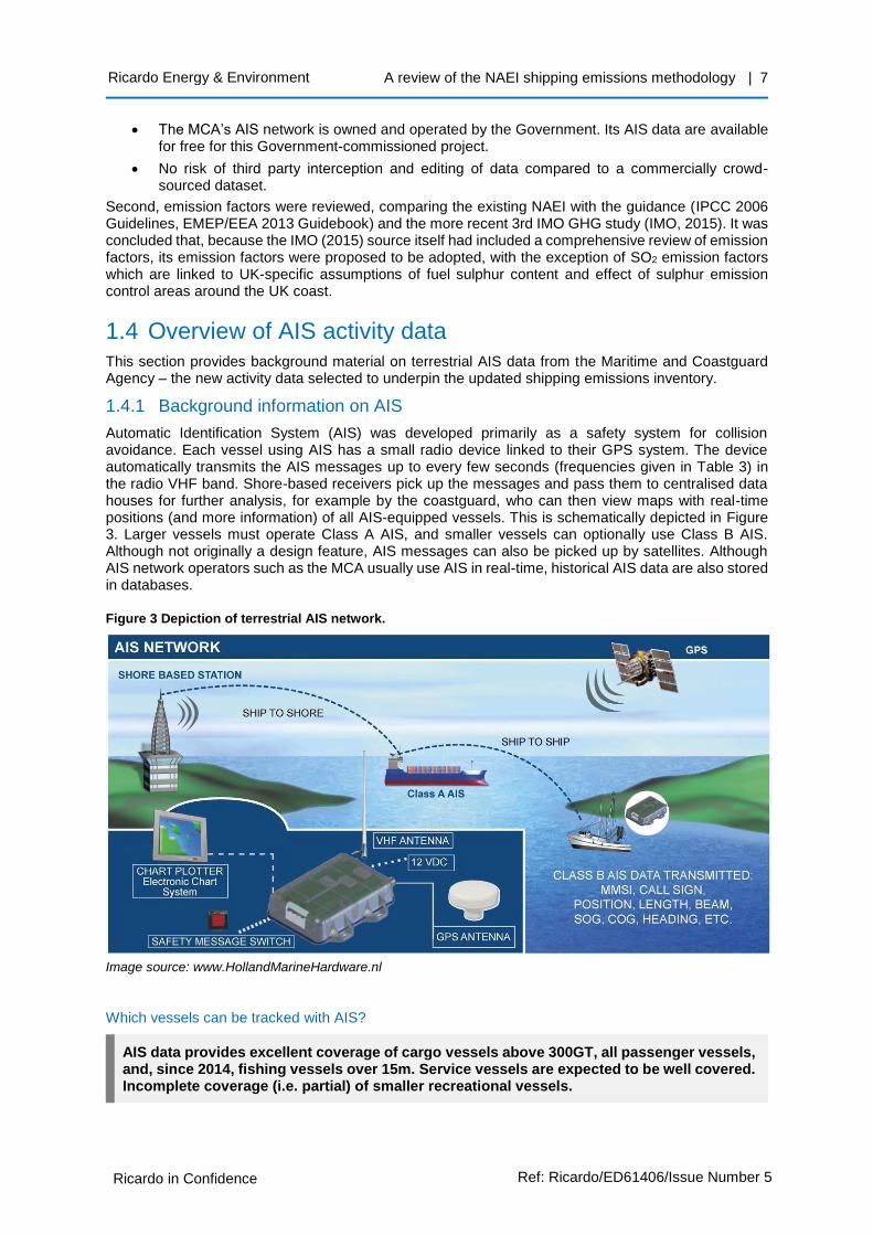
Automatic Identification System (AIS) was developed primarily as a safety system for collision avoidance. Each vessel using AIS has a small radio device linked to their GPS system. The device automatically transmits the AIS messages up to every few seconds (frequencies given in Table 3) in the radio VHF band. Shore-based receivers pick up the messages and pass them to centralised data houses for further analysis, for example by the coastguard, who can then view maps with real-time positions (and more information) of all AIS-equipped vessels. This is schematically depicted in Figure 3. Larger vessels must operate Class A AIS, and smaller vessels can optionally use Class B AIS. Although not originally a design feature, AIS messages can also be picked up by satellites. Although AIS network operators such as the MCA usually use AIS in real-time, historical AIS data are also stored in databases.
Figure 3 Depiction of terrestrial AIS network.
Image source: www.HollandMarineHardware.nl
Which vessels can be tracked with AIS?
AIS data provides excellent coverage of cargo vessels above 300GT, all passenger vessels, and, since 2014, fishing vessels over 15m. Service vessels are expected to be well covered. Incomplete coverage (i.e. partial) of smaller recreational vessels.

A review of the NAEI shipping emissions methodology | 8
Ricardo in Confidence Ref: Ricardo/ED61406/Issue Number 5
Ricardo Energy & Environment
The requirements to carry and use AIS equipment are laid down in the IMO’s Safety of Life at Sea (SOLAS) Convention and supplemented in the EU by Directive 2011/15/EU amending Directive 2002/59/EC establishing a Community vessel traffic monitoring and information system. This is implemented in the UK through The Merchant Shipping (Vessel Traffic Monitoring and Reporting Requirements) Regulations 2004 (as amended). The vessel categories in Table 2 are required to use (Class A) AIS.
Table 2 Class A AIS requirements
Vessel category
Requirement to fit AIS Class A
Cargo vessels
All vessels over 300 GT on international voyages
Passenger vessels
All vessels. But Member States can exempt passenger vessels that are either <15m length or <300GT and which are engaged on non-international voyages from this requirement. It is unclear to what extent this exemption has been implemented and thus affecting vessels travelling in UK waters.
Fishing vessels
All vessels with overall length >15m as follows:
• Existing vessels >24m should have been fitted by 31 May 2012
• Existing vessels 18m to 24m should have been fitted by 31 May 2013
• Existing vessels 15m to 18m should have been fitted by 31 May 2014
• new-built fishing vessels >15m should have been fitted from 30 November 2010
Other, naval No requirement.
There are no regulatory requirements on vessels not covered in Table 2 to fit AIS, i.e. including fishing vessels <15m, cargo vessels <300GT and leisure craft. Port authorities typically equip their port service vessels including tugs with AIS. However, many vessel operators may voluntarily choose to equip their vessels with AIS, typically the cheaper and lower power Class B devices, for safety benefits. The proportion of other, smaller vessels that choose to fit Class B devices is unknown. Class B AIS messages are only broadcast when there is sufficient bandwidth on the AIS channel. AIS data therefore has partial coverage of vessels smaller than 300 GT. Specifically for leisure craft, section 2.4.7 indicates that coverage of recreational vessels including inland waterways may be as low as 3% to 8%.
Even with AIS fitted, a vessel can only be tracked if the AIS transmitter is switched on. The practice of fishing vessel operators turning off their AIS transponders has been documented and investigated, meaning that there could be periods with large gaps between messages, increasing uncertainty in using the data for emission estimates.6 However, it is assumed that close to the UK, the close oversight by the MCA will mean that such practices of turning off AIS transponders will be very rare within the range of the MCA’s AIS receivers. There may also be legitimate reasons for gaps between consecutive AIS messages, for example if a vessel was simply out of range of all AIS receivers, or if the receiver reached its maximum bandwidth capacity.
The technology used to receive AIS messages has defined algorithms to deal with situations when more AIS messages are broadcast than can be received (bandwidth exceedance). The algorithm prioritises Class A AIS messages over Class B messages, and also discards AIS messages from vessels furthest away from the receiver. Hence not all vessel AIS messages transmitted are recorded, but capacity constraints are likely to only be reached in the busiest shipping lanes such as the English Channel. This may reduce the temporal granularity of AIS position reports below the maximum of every few seconds, but is not considered a limiting factor for emission inventory development because when vessels are at sea, they travel at relatively constant speeds and in relatively straight lines, such that temporally less precise data will have low uncertainty. Marine Scotland (2014) conclude that much more AIS data is transmitted than received, but that this does not limit the ability to track vessels’ movements with sufficient accuracy.
6 For example, the Global Fishing Watch at http://blog.globalfishingwatch.org/2016/07/going-dark-when-vessels-turn-off-ais-broadcasts/

A review of the NAEI shipping emissions methodology | 9
Ricardo in Confidence Ref: Ricardo/ED61406/Issue Number 5
Ricardo Energy & Environment
What information is transmitted in AIS messages and how frequently are they transmitted?
AIS data offer high accuracy tracking of vessel positions. The data are transmitted more frequently than needed for an emission inventory. Supplementary parameters such as vessel speed and draught are reported, which can help refine estimates of engine load.
There are two types of AIS messages – the more frequently generated position report messages, and the less frequently transmitted voyage data messages. Multiple data are encoded in AIS messages; some data are automatically generated from on-board equipment whilst others are manually entered. Table 3 summarises the contents of Class A AIS messages. Class B AIS transmits position and voyage messages less frequently than Class A (every 5 seconds to every 3 minutes), although this is still with sufficient frequency for the purposes of tracking movements for inventory compilation. Full lists of AIS message data content is included in Appendix 1.
Vessels are uniquely identified based on MMSI number – the maritime mobile service identity number. This should be a 9-digit code, and, for vessels, should begin with one of the digits 2 to 7.7 The first three digits are allocated to a region or country. The UK registered vessels should be allocated MMSI numbers that begin with 232, 233, 234 or 235. IMO is also a unique identifier for the vessel, which is a 7-digit code.
Table 3 AIS position and voyage message contents
Data origin Position Report Ship static and voyage related data
Message identifier 1, 2 or 3 (Class A)
18 (Class B)
5 (Class A)
24B (Class B)
Automatic transmission
frequency
Every 2 to 10 seconds while underway depending on speed; every 3 minutes while at anchor (Class A)
Every 5 seconds to 3 minutes depending on speed (Class B)
Every 6 minutes
Automatically reported data from on-board equipment
(high accuracy)
Message repeat indicator Latitude, Longitude, Position accuracy Speed over ground (SOG), Course over ground (COG), Rate of turn (Class A only) True heading, Timestamp
Message repeat indicator
Manually entered by vessel operator, typically once
MMSI number (ID)
MMSI number (ID) IMO number (ID) (Class A only) Call sign Name of vessel (Class A only) Type of ship and cargo type Dimensions of vessel
Manually entered by vessel operator every voyage
(lower accuracy)
Navigational status (Class A only) Special manoeuvre indicator (Class A only)
Estimated time of arrival (Class A only) Destination (Class A only) Draught (Class A only)
7 Other maritime allocations of the first MMSI number digit are: 0: Ship group, coast station, or group of coast stations 1: Search and rescue aircraft 8: Handheld VHF transceiver 9: Devices using a free-form number identity

A review of the NAEI shipping emissions methodology | 10
Ricardo in Confidence Ref: Ricardo/ED61406/Issue Number 5
Ricardo Energy & Environment
Are the AIS messages that are received correct?
There is high confidence in the spatial data in AIS messages. Some parameters included in AIS messages are subject to human error.
The AIS information on position, course and speed are automatically reported from ships’ instruments without human intervention and should be correct at transmission. The accuracy of AIS position data depends on the accuracy of navigation equipment on each vessel. Vessels’ navigation equipment accuracy can be expected to be high due to annual testing requirements of such data imposed by the SOLAS Convention (Chapter V, Regulation 18.9). However, errors may still occur with the positioning system leading to inaccurate position data (MMO, 2014). Overall, there is high confidence in the spatial information of AIS (MMO, 2013).
Some information included in AIS messages is manually entered into the AIS instrument and therefore has limitations due to operator error or misrepresentation of information. These are listed in the lower rows of Table 3. The types of information that are manually entered once during setup rather than frequently are prone to lower error rates – for example MMO (2013) estimated error levels in MMSI number and ship type at 2% of entries. The information manually entered for each voyage are prone to higher levels of error – for example MMO (2013) estimated data on ship draught was erroneous8 for 35% of entries.
In addition to inadvertent mistakes in AIS reported data, it is also possible for AIS data to be purposefully altered (Balduzzi et al., 2014). AIS messages could be subject to various spoofing and hijacking threats, and also that threats exist that may disrupt the availability of receivers. The extent to which AIS data that are received have been subject to malicious medication or otherwise is not known. Neither is the extent to which receivers’ availability has been maliciously targeted. This risk has been minimised through the choice of Government-owned AIS network data.
1.4.2 Further information on terrestrial AIS data from the MCA
Overview of data provided by the MCA
Class A and Class B data from one (former) MCA database system – calendar year 2014; Class A and Class B data from second (new) MCA database system – Sept - Dec 2014.
The MCA provided calendar year 2014 class A and class B terrestrial AIS data in an encoded 6-bit binary format. In all, these data were around 2 billion AIS messages, stored in text files totalling around 260 GB. Class A and Class B data were provided in separate files. The different types of AIS messages (position and voyage messages) were not separated.
During 2014, the MCA’s AIS data storage network comprised two systems (‘legacy’ and ‘FCG’) as they transitioned to a new storage system. To ensure a complete dataset for this study, the MCA provided data from both their systems for certain months of the year as during September, October and November neither of the MCA’s systems recorded all the UK AIS data. The MCA informed us that combining the two systems’ data would produce a complete activity dataset. The following data were provided:
• ‘Legacy’ system: data for the calendar year 2014, in one csv file per week per class
• ‘FCG’: data for four months September to December 2014, in one csv file per month per class
The data received from the MCA unexpectedly included coverage from terrestrial receivers along foreign (Spanish, French, Belgian, Dutch, German, Danish and Norwegian) coastlines, presumably due to the MCA’s data sharing agreement via EMSA (see Figure 5).
Activity data for an entire calendar year was used rather than using vessel activity data for discrete weeks distributed around the calendar year as being representative of an entire year of activity and appropriate scaling up. This choice was made to minimise uncertainty in allocation of emissions between domestic and international voyages that would otherwise span the discrete time periods being analysed and not analysed. This uncertainty was identified in MMO (2013) and MMO (2014).
8 Erroneous was taken to be outside +/- 20% tolerance of data recorded in Southampton Port’s Vessel Information System

A review of the NAEI shipping emissions methodology | 11
Ricardo in Confidence Ref: Ricardo/ED61406/Issue Number 5
Ricardo Energy & Environment
From an air quality point of view, using satellite AIS data to complement terrestrial AIS data brings little benefit in improving the quantification of pollutants emitted most closely to the UK shores in spite of its coverage spanning a greater range off the UK coastline.
What is the theoretical range of terrestrial AIS?
Terrestrial AIS data should provide near complete coverage within 12nm of the UK coastline (UK territorial waters) but incomplete coverage to 200nm (exclusive economic zone).
AIS messages are sent as VHF radio signals, which are limited to line-of-sight (plus diffraction effects) and are affected by atmospheric conditions. Terrestrial AIS receivers can typically pick up Class A AIS messages from vessels that are up to 30-50 nautical miles (nm) away, and Class B AIS messages from vessels up to 10-15 nautical miles away. The range is affected by the height of the transmitter on the vessel and the height of the receiver above water. The range can decrease during poor atmospheric conditions (e.g. Class A down to 20 nautical miles) yet may extend to several hundred nautical miles from high antenna during specific atmospheric conditions (MMO, 2014). This variability according to the weather means that coverage of a terrestrial-AIS dataset varies during a calendar year. Landmass also affects signals. The placement of where receivers are located limits where vessels can be tracked.
These ranges mean that terrestrial AIS data on its own should provide complete coverage of vessels within UK territorial waters of 12nm from the coastline, assuming receiver stations provide coverage around the entire coastline. Terrestrial AIS data are not expected to provide complete coverage of all shipping activity up to the 200nm limit of the exclusive economic zone, although, importantly, most domestic activity from AIS Class A and B is expected to be captured. This is because vessels on UK domestic voyages, aside from fishing vessels and those servicing offshore oil & gas platforms, may be expected to remain within 60 miles from the UK coastline to be able to receive emergency assistance from the coastguard.9
What coverage does the MCA’s terrestrial AIS network provide?
The MCA’s terrestrial AIS receiver network has coverage all around the UK coastline and so should provide near complete coverage of coastwise UK domestic voyages. Coverage is expected to be incomplete for vessel journeys to some offshore oil/gas platforms or fishing in non-UK waters.
Vessels travelling between the UK and the Crown Dependencies of Jersey, Guernsey and the Isle of Man are covered by the MCA terrestrial AIS data.
Vessels travelling between the UK and the Overseas Territories (and domestically within the Overseas Territories) are not covered by the MCA terrestrial AIS data.
The Maritime and Coastguard Agency (MCA) is responsible for operating the UK’s own terrestrial AIS data network to meet the requirement of monitoring vessels over 300 GT of the Vessel Traffic Monitoring Directive. In practice, the MCA’s navigational safety branch shares its AIS data with other countries via the European Maritime and Safety Agency (EMSA) and in turn accesses AIS data from those other countries integrated with its own AIS data.
The MCA’s exclusive network of receiver stations aims to provide a comprehensive reception coverage around the UK coastline. The locations of the MCA’s receivers as of 2014 are shown in Figure 4, each of which is shown with 10nm and 20nm radii to show theoretical normal reception of AIS-B messages, and small AIS-A vessels (e.g. fishing vessels), respectively. Figure 4 also shows a blue line marking the collective coverage for the typical class A vessels (40nm reception of each receiver). The 2014 Class A and B AIS data provided by the MCA for the study are shown in Figure 5. Comparing the indicative reception range of 40nm shown in Figure 4 with the MCA data in Figure 5 suggests that the terrestrial AIS data from the MCA ought to offer very good coverage of coastwise UK domestic movements as the data show spatial coverage significantly beyond the theoretical average limit in Figure 4.
9 Personal communication, MCA, 27 July 2017, and MCA (2003)

A review of the NAEI shipping emissions methodology | 12
Ricardo in Confidence Ref: Ricardo/ED61406/Issue Number 5
Ricardo Energy & Environment
Figure 4 Indicative 40nm reception range of MCA AIS receiver network shown by the blue solid line suggests largest gaps of coverage of the exclusive economic zone is in the North Sea, southwest of Cornwall and north/west of the Outer Hebrides (source: Marine Scotland, 2014)
Figure 5 Class A (left) and B (right) position report density per km2 in 2014 after downsampling to 5 minute intervals (data source: MCA terrestrial AIS)
A review of the NAEI shipping emissions methodology | 13
Ricardo in Confidence Ref: Ricardo/ED61406/Issue Number 5
Ricardo Energy & Environment
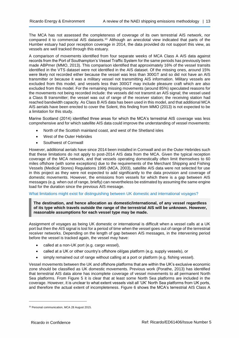
The MCA has not assessed the completeness of coverage of its own terrestrial AIS network, nor compared it to commercial AIS datasets.10 Although an anecdotal view indicated that parts of the Humber estuary had poor reception coverage in 2014, the data provided do not support this view, as vessels are well tracked through this estuary.
A comparison of movements identified from four separate weeks of MCA Class A AIS data against records from the Port of Southampton’s Vessel Traffic System for the same periods has previously been made ABPmer (MMO, 2013). This comparison identified that approximately 16% of the vessel transits identified in the VTS dataset were not identified in the AIS dataset. Of the missing ones, around 15% were likely not recorded either because the vessel was less than 300GT and so did not have an AIS transmitter or because it was a military vessel not transmitting AIS information. Military vessels are excluded from this model, and vessels less than 300GT may include pleasure craft which are also excluded from this model. For the remaining missing movements (around 85%) speculated reasons for the movements not being recorded include: the vessels did not transmit an AIS signal; the vessel used a Class B transmitter; the vessel was out of range of the receiver station; the receiving station had reached bandwidth capacity. As Class B AIS data has been used in this model, and that additional MCA AIS aerials have been erected to cover the Solent, this finding from MMO (2013) is not expected to be a limitation for this study.
Marine Scotland (2014) identified three areas for which the MCA’s terrestrial AIS coverage was less comprehensive and for which satellite AIS data could improve the understanding of vessel movements:
• North of the Scottish mainland coast, and west of the Shetland isles
• West of the Outer Hebrides
• Southwest of Cornwall
However, additional aerials have since 2014 been installed in Cornwall and on the Outer Hebrides such that these limitations do not apply to post-2014 AIS data from the MCA. Given the typical reception coverage of the MCA network, and that vessels operating domestically often limit themselves to 60 miles offshore (with some exceptions) due to the requirements of the Merchant Shipping and Fishing Vessels (Medical Stores) Regulations 1995 (MCA, 2003), satellite AIS data were not selected for use in this project as they were not expected to add significantly to the data provision and coverage of domestic movements. However, the emissions from vessels for which there is a gap between AIS messages (e.g. when out of range, briefly) can nevertheless be estimated by assuming the same engine load for the duration since the previous AIS message.
What limitations might exist for distinguishing between UK domestic and international voyages?
The destination, and hence allocation as domestic/international, of any vessel regardless of its type which travels outside the range of the terrestrial AIS will be unknown. However, reasonable assumptions for each vessel type may be made.
Assignment of voyages as being UK domestic or international is difficult when a vessel calls at a UK port but then the AIS signal is lost for a period of time when the vessel goes out of range of the terrestrial receiver networks. Depending on the length of gap between AIS messages, in the intervening period before the vessel is tracked again, the vessel may have:
• called at a non-UK port (e.g. cargo vessel),
• called at a UK or other country’s offshore oil/gas platform (e.g. supply vessels), or
• simply remained out of range without calling at a port or platform (e.g. fishing vessel).
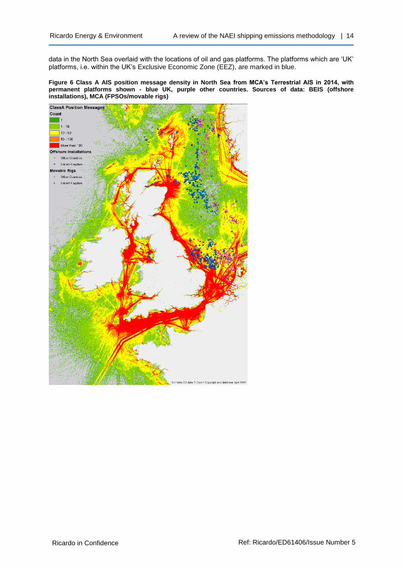
Vessel movements between the UK and offshore platforms that are within the UK’s exclusive economic zone should be classified as UK domestic movements. Previous work (Porathe, 2013) has identified that terrestrial AIS data alone has incomplete coverage of vessel movements to all permanent North Sea platforms. From Figure 5 it is clear that at least some North Sea platforms are included in the coverage. However, it is unclear to what extent vessels visit all ‘UK’ North Sea platforms from UK ports, and therefore the actual extent of incompleteness. Figure 6 shows the MCA’s terrestrial AIS Class A
10 Personal communication, MCA 28 August 2015.
A review of the NAEI shipping emissions methodology | 14
Ricardo in Confidence Ref: Ricardo/ED61406/Issue Number 5
Ricardo Energy & Environment
data in the North Sea overlaid with the locations of oil and gas platforms. The platforms which are ‘UK’ platforms, i.e. within the UK’s Exclusive Economic Zone (EEZ), are marked in blue.
Figure 6 Class A AIS position message density in North Sea from MCA’s Terrestrial AIS in 2014, with permanent platforms shown - blue UK, purple other countries. Sources of data: BEIS (offshore installations), MCA (FPSOs/movable rigs)

A review of the NAEI shipping emissions methodology | 15
Ricardo in Confidence Ref: Ricardo/ED61406/Issue Number 5
Ricardo Energy & Environment
2 Revised shipping emissions inventory – base year 2014
2.1 Summary of modelling approach
Overview of new methodology
The new NAEI shipping model methodology is similar to the existing NAEI approach in that fuel consumption and emissions are estimated in detail for a base year (in this case, 2014), and less detailed shipping activity statistics are used as the main driver to estimate emissions and fuel consumption for past years and up to the current year. Future shipping fuel consumption and emissions are estimated using assumed activity growth rates among considerations of emission factors.
The new shipping model emission calculation – of multiplying an emission factor expressed in grams per kWh by estimated engine demand in kWh – is also similar to existing NAEI estimates that are based on Entec (2010). In this sense, the new model methodology meets the requirements of Tier 3 in the EMEP EEA Guidebook 2016. The new bottom-up methodology calculates fuel consumption and emissions for each vessel. The methodology goes beyond the Tier 3 approach set out in the Guidebook by calculating fuel consumption and emissions for each part of a voyage using AIS data, rather than carrying out the calculation for each port-to-port voyage as a whole. The use of AIS data to support an emission inventory follows the same practice as the work by the IMO in its 3rd GHG study (IMO, 2015). Many of the assumptions used in the modelling have been drawn from the IMO’s work (IMO, 2015).
The emissions are calculated separately for each vessel and for each AIS data point, accounting for the time duration until the next AIS data point, assuming that the vessel continues to combust fuel and emit pollution at the same rate until the subsequent AIS message. The fuel consumption and emission factors are tailored to the specific vessel that is identified in the AIS dataset. The factors account for:
• The fuel type assumed to be used by the vessel, the known engine type and speed (rpm).
• The rated power of the engines, which are either known from a 3rd party database, or estimated based on other known or reported vessel characteristics (e.g. vessel length)
• The actual power demands on the main engines for each AIS message, expressed as a function of reported and designed vessel speed, and reported and designed vessel draught.
• The location and type of the vessel, i.e. whether the vessel is in a SECA, whether the vessel is at berth, and whether the vessel is a passenger vessel.
The new model methodology separates vessel movements into domestic, international and passing the UK (transit). This new domestic estimate will be used for UK reporting of national emission totals in inventory submissions to the UNFCCC, UNECE/CLRTAP and EU NECD. The model’s estimates of international shipping emissions are not proposed to be used for UK reporting, which is further described in section 4.
Due to the considerable complexity of the modelling required for this inventory, it is recommended that this exercise is not repeated each year but rather, for example, every five years. Similarly, to the previous approach taken for the NAEI shipping emission inventory, intermediate years before a subsequent full-bottom-up re-modelling can continue to use the same approach as for back-casting.
Benefits of the new methodology beyond the existing NAEI approach
The new model methodology is more sophisticated than the existing NAEI shipping emissions approach, and goes beyond the Tier 3 methodology described in the EMEP EEA Guidebook 2016. The following improvements are realised:
• More complete activity dataset. The switch in choice of activity dataset from a port to port database used in Entec (2010) that focuses on internationally trading vessels to an AIS activity dataset provides improved domestic vessel coverage, particularly of those vessel types with previously poor coverage. This includes, in particular, offshore industry vessels, fishing boats, passenger ferries and service craft.

A review of the NAEI shipping emissions methodology | 16
Ricardo in Confidence Ref: Ricardo/ED61406/Issue Number 5
Ricardo Energy & Environment
• Spatially resolved activity dataset. The AIS dataset shows the actual locations of vessels, meaning emission estimates can be spatially resolved to a high resolution. This compares with the previous shipping inventory (Entec, 2010) which estimated routings of vessel voyages.
• Improved emission calculation accuracy of main engines. The calculation of fuel consumption and emissions of vessels now accounts for the actual speed of the vessel at any given point, rather than assuming that vessels always travel at their designed speed as was assumed in Entec (2010). The emission calculation also now uses the reported draught of the vessel to estimate engine load factor. This enhances the Tier 3 approach by making use of the data reported under AIS. Thus, the approach allows for variation in speed and load at points during the voyage rather than a single voyage average, which in turn provides a more realistic estimation of the spatial distribution in the emissions.
• Improved emission calculation accuracy of auxiliary engines. Auxiliary engine power demand, previously modelled in Entec (2010) with static assumptions, is now varied by vessel category, size and by mode.
• Now accounts for fuel consumption and emissions from auxiliary boilers. This emission source, used on board larger vessels for heating and hot water production, was not previously estimated in the Entec (2010) model.
• More vessel types are distinguished. Vessel type and size classification have been aligned with the IMO classification. This has 47 categories after splitting by size and type, compared to eight in Entec (2010). Separate assumptions are made for the fuel and emission calculations by category. Several new categories of vessels are now stipulated compared to previously, including in particular offshore industry vessels, subcategories of service vessels and cruise vessels.
• Improved estimate accuracy for vessels starting and finishing at the same port. Vessels that start and finish at the same port are treated in the same way as other vessels in this new model. Their emissions are estimated and spatially resolved. The previous shipping model in Entec (2010) was limited to high-level estimates of such voyages, and they were not spatially resolved.
• Crown dependencies are now specifically included. Emissions associated with movements among and to/from the three crown dependencies can be distinguished.
New base year model map
A model map of the base year methodology is shown in Figure 7. In summary, the first five stages are steps needed to process the raw AIS data. Stages 6 fills in gaps in an external database of vessel characteristics. Stage 7 of the methodology estimates the emissions from the main engine, auxiliary engine and if applicable the auxiliary boiler of the vessel identified in each geolocated AIS message.
In Stage 8, each AIS message is considered within a string of AIS messages, or ‘passage’. The start AIS message and end AIS message of the passages are used to determine whether each passage, and by extension each AIS message, is categorised as UK domestic, UK international, allocated to Crown Dependencies or is a passing transit not calling at the UK. The final model stage re-merges the emissions calculated with the geographical allocation.

A review of the NAEI shipping emissions methodology | 17
Ricardo in Confidence Ref: Ricardo/ED61406/Issue Number 5
Ricardo Energy & Environment
Figure 7 Base year modelling stages
2.2 Detailed methodology description
This section summarises the methodology for the new NAEI shipping emissions inventory.
2.2.1 Stage 1: decode raw AIS data
The first stage of the model is to decode the provided AIS data. The AIS data received from the MCA was in a raw encoded format shown in the first Box below, in text files.
During 2014, the MCA’s AIS data storage network comprised two systems as they transitioned to a new storage system. To ensure a complete dataset for this study, the MCA provided data from both their systems for certain months of the year as during September, October and November neither of the MCA’s systems recorded all the UK AIS data. The MCA recommended, to produce a complete activity dataset, to combine the two system’s data. The following data were provided:
• ‘Legacy’ system: data for the calendar year 2014, in one text csv file per week per class
• ‘FCG system’: data for the four months September to December 2014, in one csv file per month per class
Format and example of provided Class A and Class B messages
Class A
YYYY-MM-DD HH:MM:SS,[MMSI],[AIS message number],[Encoded message][white space]
2014-04-29 00:00:00.000,[MMSI],1,13Ok;V000Nwo6cfQMGWlKCJ02<0@
Class B
YYYY-MM-DD HH:MM:SS,[MMSI],[Encoded message]
2014-10-29 00:00:00.000,[MMSI],H3P;tN4N4I138D0j3I4n000H;220

A review of the NAEI shipping emissions methodology | 18
Ricardo in Confidence Ref: Ricardo/ED61406/Issue Number 5
Ricardo Energy & Environment
The encoded message is in 6 bit ASCII code. The date/time stamp in the provided message from the MCA is the date/time stamp of when the message was received by the AIS mast receiver. The contents of AIS encoded messages are set out in Appendix 1.
A previous study carried out for the Marine Management Organisation generated open source software to decode AIS data that are provided by the MCA (MMO, 2014). The Stage 1 Processor of this open source software was used to decode the text files of encoded messages. The decoder outputs an unsorted csv file which contains many different message types and hence does not include column header information.
It was identified that since the MMO decoding software was published the format of the Class A AIS data provided by the MCA has subtly changed. The result of this is that some pre-processing of the encoded Class A AIS data was first required before using the decoding software to remove the [AIS message number] and [white space]. It will be important to note for future use of the MMO decoding software to ensure the exact formatting of AIS messages.
The AIS message format required for the decoder (contrary to the documentation for the decoder) is shown in the Box below:
Format and examples of Class A and Class B messages for decoder
Class A
YYYY-MM-DD HH:MM:SS,[MMSI],[Encoded message]
2014-04-29 00:00:00.000,[MMSI],13Ok;V000Nwo6cfQMGWlKCJ02<0@
Class B
YYYY-MM-DD HH:MM:SS,[MMSI],[Encoded message]
2014-10-29 00:00:00.000,[MMSI],H3P;tN4N4I138D0j3I4n000H;220
In this first stage, the outputs from the decoder were split into smaller files of maximum 1 million lines per file, to facilitate processing.
QA protocols carried out for this stage included:
• Row counts of the number of encoded messages compared to the number of decoded messages.
• Use of a third party online AIS message decoder to spot-sample verify, for fictitious MMSI numbers, that the decoder outputs were correct.
2.2.2 Stage 2: sort AIS message types
The second stage of the model separates the different types of AIS messages: class A position messages (1/2/3), class A voyage messages (5), class B position messages (18), class B voyage messages (24B). Any received Class B messages 19 or 24A were discarded as not needed. Following separation into the different message types, the field headers for each comma-separated field were added.
In addition, this stage also extracts the unique IMO and MMSI numbers reported in the dataset, used to specify the vessel characteristics from the Clarksons database (see section 2.2.6).
QA protocols carried out for this stage included
• Row counts of the number of each message types compared to the number of decoded messages. The small proportion of AIS messages that failed to correctly decode were logged.
• Spot sample verification of the correct column headers applied to the fields.
2.2.3 Stage 3: Thin and clean AIS position messages
The third model stage aims to reduce the size of the activity dataset to make it more manageable to work with for calculating emissions. Without doing so, the processing times were expected to be measured in weeks rather than days. This stage removes AIS fields not needed for the calculations, removes data identified as erroneous, and temporally down-samples the AIS position database. In

A review of the NAEI shipping emissions methodology | 19
Ricardo in Confidence Ref: Ricardo/ED61406/Issue Number 5
Ricardo Energy & Environment
particular, the temporal density of position messages, particularly for Class A, was very high, up to one every few seconds for each vessel, leading to a larger than necessary activity dataset.
The first step removes many of the AIS data fields that are simply not needed for the subsequent emission inventory calculations. The fields that were removed were as follows:
• Class A fields:
o Position messages (message type 1/2/3)
▪ User_ID [as this is a repeat of MMSI_number]
▪ Special_manoeurvre_indicator
▪ spare
▪ RAIM_flag
▪ communication_state
o Voyage messages (message type 5)
▪ User_ID [as this is a repeat of MMSI_number]
▪ AIS_version_indicator
▪ type_of_position_fixing_device
▪ data terminal_ready
▪ spare
• Class B fields:
o Position messages (message type 18)
▪ Spare_1
▪ User_ID [as this is a repeat of MMSI_number]
▪ Spare_2
▪ class_B_unit_flag
▪ class_B_display_flag
▪ class_B_DSC_flag
▪ class_B_band_flag
▪ class_B_Message_22_flag
▪ mode_flag
▪ RAIM_flag
▪ communication_state_selector_flag
▪ communication state
o Voyage messages (message type 24b)
▪ user_id [as this is a repeat of MMSI number]
▪ spare
The second step in this stage removes duplicate messages. Duplicate AIS messages may occur in the dataset if the vessel has broadcast the message multiple times, or if multiple AIS receivers received the message. This step identifies in class A position messages and class B position messages which of these are completely identical (i.e. including the same geographic coordinates and the same time stamp) and leaves only one version of that message.
The third step identifies data which appear to be unreasonable, and so are flagged as being erroneous to enable them to be filtered out in subsequent steps. These data may occur due to erroneously functioning AIS equipment on the vessel, errors introduced due to reception cover, or AIS message decoding failures during Stage 1 of the model. The specific data flagged in this step include:
• Position messages with invalid geographic coordinates, such as null, or equal to 0 or 1.
• Position messages and voyage messages with erroneous date and time fields, i.e. not occurring in 2014.
• Position messages with reported speed over ground over 50 knots. The cut-off of 50 knots was selected as very few vessels (other than speed boats) can reach these speeds.
A review of the NAEI shipping emissions methodology | 20
Ricardo in Confidence Ref: Ricardo/ED61406/Issue Number 5
Ricardo Energy & Environment
• Position messages with geographic coordinates which imply a speed over 50 knots from the previous position message from the same MMSI number given the time difference between the consecutive position messages. This is most likely due to erroneous coordinates.
The fourth step temporally down-samples AIS position messages of vessels which are moving. In line with IMO (2015), the assumption is made that vessels with reported speed over ground of less than 1 knot are stationary (which can include at berth or at anchor), and those with reported speed 1 knot or more are moving.11
It was necessary to decide how much to down-sample the data with a direct trade-off between dataset size and inventory accuracy. Two down-sampling temporal resolutions were investigated: down-sampling to 1 message every minute and to 1 message every 5 minute. For comparison, IMO (2015) used an AIS dataset of one message per hour.
Figure 8 and Figure 9 show two examples of the two down-sampling temporal resolutions. Comparing the two resolutions indicates that down-sampling at 1 message every 5 minutes loses some geographical precision of the location of emissions, as high rates of turn at the mouth of the River Yare and approaching Rosslare are not closely captured. It should not be inferred that the model ‘spreads’ the emissions along the marked tracks of the vessel as this is not done; rather, the emissions are modelled as occurring at the specific points (single latitude and longitude) of the locations of the position messages. Hence, there will be a small disadvantage to air quality modelling by downsampling at 5-minute resolution rather than 1 minute resolution. This is nevertheless still a considerable improvement on the existing inventory, and is higher temporal resolution than used in IMO (2015).
Overall, the contribution to total emissions of a vessel journey of the portion when they manoeuvre coming in to port is small because that part of the voyage is a small proportion of the journey and because the main engines are operating at lower load. It is also offset by the higher emissions when vessels manoeuvre going out of a port at higher load. Consequently, it is considered that the disadvantage in accuracy associated with down-sampling to 5 minutes rather than 1 minute is minor from an inventory perspective compared to the processing time benefits of working with a significantly smaller dataset. It is noted that the majority of emissions from vessels occur when they are (a) at higher speeds and (also, hence) (b) travelling in straighter lines, for which a lower temporal resolution is sufficient.
Lower temporal resolution (e.g. 5 minutes rather than 1 minute) leads to less accurate tracking when vessels change speed (emissions) and course (location of emissions). To some degree however, the effects on emissions estimation is less significant when the overall effects of vessels accelerating and decelerating are taken into account. When vessels are accelerating, the calculation will underestimate emissions as the speed at the start of the (5 minute) period will be used to estimate emissions over the entire 5-minute period. In a similar way, when vessels are decelerating, the calculation will over-estimate emissions. These two effects, when considered over an entire vessel journey, should cancel each other out if the absolute rates of acceleration and deceleration are similar. Hence total estimates should be less affected than the geographical distribution.
The option of retaining higher temporal resolution close to shore and lower temporal resolution further from shorelines was considered, for example, a mixture of 1-minute and 5-minute resolution. However, this was rejected on the basis of complexity of algorithm development and implementation.
In conclusion, the temporal resolution of 5 minutes was adopted in the model. The model selects one position message at random from those available in every 5-minute period.
11 Vessels can still report speeds above zero whilst at anchor due to currents.

A review of the NAEI shipping emissions methodology | 21
Ricardo in Confidence Ref: Ricardo/ED61406/Issue Number 5
Ricardo Energy & Environment
Figure 8 Down-sampling example – Great Yarmouth. Left hand plot shows one week of one vessel in July 2014 down-sampled to 1 message per minute. Right hand plot shows multiple vessels for the same period, but down-sampled to 1 message per 5 minutes.
Figure 9 Down-sampling example – Rosslare. Left hand plot shows one week of one vessel in July 2014 down-sampled to 1 message per minute. Right hand plot shows the same vessel for the same period, but down-sampled to 1 message per 5 minutes.
The fifth step temporally thins the AIS position messages of vessels which are stationary. Stationary vessels are those reporting speeds of less than 1 knot. This process identifies all consecutive messages that are stationary for a given MMSI, and removes all intermediate positions, retaining the first and the last stationary message of this vessel. With this approach, the vessel is assumed to remain stationary until the next stationary AIS position message.
QA protocols carried out for this stage included:
• Row counts of the number of messages thinned and cleaned
• Check for erroneous messages remaining in the dataset.
• Visual inspection of mapped position messages against land
• Map inspection that Legacy and FCG data combined.
2.2.4 Stage 4: Merge AIS voyage messages into position messages
The fourth stage of the modelling adds information available in the less-frequently transmitted AIS voyage messages to the more frequently transmitted AIS position messages. The purpose of this is to have all information necessary for the emission calculation available for each AIS message. The fields extracted from the voyage messages that are matched to the position messages are:
© OpenStreetMap contributors © OpenStreetMap contributors
© OpenStreetMap contributors © OpenStreetMap contributors
A review of the NAEI shipping emissions methodology | 22
Ricardo in Confidence Ref: Ricardo/ED61406/Issue Number 5
Ricardo Energy & Environment
• vessel IMO number
• vessel length and breadth
• type of ship and cargo
• voyage draught
The method used to identify and match the relevant voyage message for each position message categorises each down-sampled position message into a five minute “block”, for example the 5-minute period beginning at 17:05 and ending at 17:10. The same process is carried out for the voyage messages, of assigning them to the nearest five minute period. The tables and messages are then matched using the unique combinations of the reported MMSI number together with the unique five-minute period. This process therefore selects the nearest available voyage message to the timestamp of each position message. It therefore selects in some cases the voyage message that precedes a position message. Given the fields extracted from the voyage message database (by definition) infrequently change, this is not considered to be a limitation.
QA protocols carried out for this stage included:
• Manual spot sampling check that 5 minute period is correct match from original message time.
• Check all position messages allocated details from a voyage message
2.2.5 Stage 5: Add geographic information to each AIS message
At this stage of the model a set of geographic components for each AIS position message is defined, in order to make the necessary characterisations of each vessel movement along the process. The first step was to determine the location of each message and for that the following fields were used (Longitude, Latitude). These coordinates and the rest of the mapping layers used in this analysis were imported into a GIS environment, where their projection system was verified or adjusted as appropriately to either:
• World Geodetic System 1984 (WGS84) – coordinates in decimal degrees
• OSGB 1936 / British National Grid – coordinates in metres
The first step is to allocate each position message to unique 1km grid squares, which are in line with the NAEI gridded emissions data12. This enabled the generation of outputs which were used during the process such as movement type categorisation (e.g. Domestic, International etc), model validation of assumptions and results, and the generation aggregated activity and emissions maps. An additional field was added in the position messages table, which indicated the unique grid square. Figure 10 shows a sample of position messages on top of a 1x1km polygon and how this translates to a gridded dataset with messages count.
The next geographical component assigned to each vessel location was whether the AIS message was transmitted within a Sulphur Emission Control Area (SECA) or not. The polygon for the SECA used in this study, was created based on the coordinates information published on the ECG (2013). Figure 11 indicates the extent of the SECA and the Class A AIS position message density is distributed in and out of it. Using these geographical boundaries, an additional field was generated on the AIS position messages to designate the appropriate information for the emissions modelling.
12 http://naei.beis.gov.uk/data/gis-mapping

A review of the NAEI shipping emissions methodology | 23
Ricardo in Confidence Ref: Ricardo/ED61406/Issue Number 5
Ricardo Energy & Environment
Figure 10 Sample of AIS position messages allocated to 1x1km dataset in line with the NAEI gridded maps around the area of Southampton and Portsmouth
Figure 11 Geographic extent of the Sulphur Emission Control Area (SECA) around the UK
A review of the NAEI shipping emissions methodology | 24
Ricardo in Confidence Ref: Ricardo/ED61406/Issue Number 5
Ricardo Energy & Environment
Another important parameter of the emissions modelling was to determine whether a vessel is positioned at berth or at sea. To ascertain this, port locations were collected from 2 main sources:
• DfT UK ports database (Pers. Comm., DfT)
• World Port Index (WPI) database for ports outside the UK (NGA, 2016)
What limitations might exist for using port data from the WPI?
The coverage of the non-UK ports provided by the WPI is constrained to the large international ports. As a result, the international emissions from the vessels at berth may be underestimated, specifically in smaller non-UK ports not listed in the WPI. As shown in Figure 12, DfT’s ports database contains a detailed list of ports around the UK. Therefore, the emissions from vessels at berth around the UK coast was considered more accurate when using DfT data.
The port locations from the above sources are defined as single points. The spatial extent of where the vessels have been at berth, needed to be mapped. The resulting port boundaries have been created using a subsequent set of digitising and proximity analysis techniques:
• For the busiest UK ports, the location of the harbour and their extent were manually digitised (drawn as polygons) through reference to the areas of the port as visible with satellite imagery. This was completed for more than 35 ports, identified from DfT statistics on cargo tonnes loaded/unloaded at major UK ports, and from DfT statistics on the busiest passenger ports.
• For the smaller ports in the UK, the extent of the ports was determined using a combination proximity analysis:
a. 500 metres from the location point as defined by DfT in the UK ports database,
b. 300 metres from the coast as defined by OS Boundary LineTM 13
• For the Non-UK ports, the range of the harbour have been allocated in a similar way to that described for the UK small ports, but using a larger distance – 5000 metres – from the WPI points. This was done to capture the berth activity from the larger size international ports, but also the low-resolution coordinates in the WPI database (points are usually located in the mainland rather than near the coast). For the purpose of the allocation of voyages to non-UK voyages, the non-UK port destinations were necessary.
Figure 13 indicates an example of the first 2 techniques applied in the UK ports.
Following this step, a new field was created on the AIS position messages in order to designate whether the vessel was at berth or at sea. This indicator was applied only to the position messages which were considered to be ‘stationary’. The AIS speed over ground information was used to make this distinction. More specifically, when a vessel reported a speed of less than 1 knot, then it was considered to be stationary (aligned with IMO, 2015).
13 High Water polyline shapefile, https://www.ordnancesurvey.co.uk/business-and-government/products/boundary-line.html

A review of the NAEI shipping emissions methodology | 25
Ricardo in Confidence Ref: Ricardo/ED61406/Issue Number 5
Ricardo Energy & Environment
Figure 12 Port locations used for this study from different sources, DfT and WPI, overlaid on Class A position message density

A review of the NAEI shipping emissions methodology | 26
Ricardo in Confidence Ref: Ricardo/ED61406/Issue Number 5
Ricardo Energy & Environment
Figure 13 Southampton port area - the 2 spatial techniques to capture the location when vessels are assumed to be at berth
QA protocols carried out for this stage included:
• Proofing of polygons drawn for ports
• Sensitivity analysis of variation in distance thresholds from ports
• Mapping of position data within / outside SECAs
2.2.6 Stage 6: Fill gaps in vessel characteristics data
The emissions calculation process in Stage 8 requires vessel technical data such as ship type, designed ship’s speed, installed engine power, and ship dimensions. This stage of the model assembles the vessel technical data for the emissions calculation. The AIS data themselves partially cover ship type (to a lower level of detail) and ship dimensions. An additional dataset was necessary to identify installed main engine power, design speed and so on.
A database of 17,842 vessels’ technical characteristics was purchased from supplier Clarksons Research Services Ltd (‘Clarksons’) to cover as many of the vessels identified in the AIS dataset as possible. Clarksons provided data for a vessel if the IMO number matched or if the MMSI number matched the historical MMSI record for year 2014 (as MMSI numbers can be re-assigned).
However, some of the ships technical specifications in Clarksons database necessary to perform the emissions calculation process were missing (overall length, design speed and main engine power). A summary of the Clarksons database and the proportion of each field populated is given in Table 4.
Each MMSI number is allocated to one of the relevant ship type categories and ship size subcategories as used in IMO (2015) and listed in Table 5. The allocation to vessel type uses data about the vessel from Clarksons, or if this is missing, the ship type from AIS data is used. For the remaining vessels for which no ship type is known, these are subsequently excluded (explained further in section 2.4.6). The allocation for ship size subcategory is carried out on the basis of capacity. This may be dwt, GT or TEUs, which if missing from the database is infilled using multilinear regression. If there is insufficient data for a vessel to perform the regression, a median ship size bin is applied.

A review of the NAEI shipping emissions methodology | 27
Ricardo in Confidence Ref: Ricardo/ED61406/Issue Number 5
Ricardo Energy & Environment
Table 4 Clarksons database of vessel characteristics and % of fields populated.
Field type Field name Data type Proportion populated
Vessel identification
X01_CVN Number 100%
X03_IMO_NUMBER Number 100%
X57_MMSI_NUMBER Number 100%
Z01_CURRENT_NAME Short Text 100%
FLAG Short Text 100%
A12_YEAR_BUILT Number 100%
A13_MONTH_BUILT Number 99%
Z05_DATE_BUILT Date/Time 100%
Vessel type / categorisation
P36_VESSEL_TYPE Short Text 100%
ONLINE_REGISTER_SECTION Short Text 100%
ZY1_DESCRIPTION Short Text 100%
Vessel capacity, size
Z04_GT_estimated Number 100%
A04_DWT_TONNES Number 91%
A08_DRAFT_m Number 95%
A06_LOA_m Number 98%
A07_BREADTH_m Number 98%
A11_TEU_TOTAL_CAP Number 25%
A19_CARGO_CAP_cu_m Number 22%
K03_LANE_LENGTH_m Number 3%
B37_VEHICLE_CAP Number 6%
Z20_SPEC_VALUE Number 84%
Z21_SPEC_UNIT Short Text 100%
EB03_SPEED_knots Number 87%
Engine 1 specifications
EF01111_ENGINE_1_MODEL Short Text 100%
EF01105_ENGINE_1_DESIGNER_COMPANY Short Text 100%
EF01103_ENGINE_1_EQUIPMENT_TYPE Short Text 100%
EF01101_ENGINE_1_NUMBER Number 97%
EN14_OUTPUT_kW_TOTAL_max_value_ENGINE_1 Number 86%
EN08_SPEED_rpm_max_value_ENGINE_1 Number 92%
EN33_SFOC_SPECIFIC_FUEL_OIL_CONSUMPTION _g_per_kWh_ENGINE_1
Number 49%
EF01119_ENGINE_1_mKW Number 96%
EF01115_ENGINE_1_RPM Number 93%
EF01116_ENGINE_1_CYCLE Number 99%
EF01113_ENGINE_1_BUILT Number 12%
Engines 2, 3 specifications
[same fields as for Engine 1] - <2%
Auxiliary engines
EF02001_AUXILIARY_DERIVED_ TOTAL_ENGINE_NUMBER
Number 57%
EF02007_AUXILIARY_DERIVED_ TOTAL_ELECTRICAL_GENERATED_KW
Number 42%
Fuel consumption
EB04_MAIN_CONSUMPTION_tons_per_day Number 42%

A review of the NAEI shipping emissions methodology | 28
Ricardo in Confidence Ref: Ricardo/ED61406/Issue Number 5
Ricardo Energy & Environment
Table 5 Vessel type and capacity classification used (aligned with IMO, 2015). The new additional categories and subcategories compared to the existing inventory are shown in bold italic.
# Vessel type Number of vessel capacity / size subcategories
Capacity units
1 Bulk carrier 6 Deadweight tonnage (dwt)
3 Chemical tanker 4 dwt
4 Container 8 twenty-foot equivalent unit (TEU)
5 General cargo 3 dwt
6 Liquefied gas tanker 3 Cubic metres (cbm)
7 Oil tanker 8 dwt
9 Ferry-Pax only 2 Gross tonnage (GT)
10 Cruise 5 GT
12 Refrigerated bulk 1 dwt
13 Roll-on-roll-off (Ro-Ro) 2 GT
15 Yacht 1 -
16 Service - tug 1 -
17 Miscellaneous - fishing 1 -
18 Offshore 1 -
19 Service - other 1 -
20 Miscellaneous – other 1 -
Due to the gaps in the vessel characteristics database, an infilling algorithm was used to infill fields of overall length, capacity, design speed and main engine power where possible. This in-filling process is analogous to that used in IMO (2015) and in-fills using the outputs of regression analysis of data that is present in Clarksons. The algorithm is based on the multilinear regression created for each ship type as follows:
• Missing length data estimated from regression with beam, draught and deadweight data.
• Missing capacity data estimated from regression with beam, draught and length data.
• Missing design speed data estimated from regression with length, main engine power and deadweight data.
• Missing main engine power data estimated from regression with length, design speed and deadweight tonnage data.
The results of the gap-filling exercise in vessel technical characteristics, together with the assumptions related to auxiliary power are shown for Class A in Table 6 and for Class B in Table 7.

A review of the NAEI shipping emissions methodology | 29
Ricardo in Confidence Ref: Ricardo/ED61406/Issue Number 5
Ricardo Energy & Environment
Table 6 Class A post-infilling technical characteristics presented as averages for the vessel type and size (3285 unknown vessel categories are assumed to be fishing vessels). The figures in bold refer to total number of vessels of the main vessel category and weighted averages of the lengths, speeds and power of the vessel subcategories within each main category.
Vessel type and size subcategory
Number of vessels
Average length (m)
Average service speed (kn)
Average propulsion power (kW)
1 Bulk carrier 6311 138 13.3 5,868 1 3130 68 12.4 1,384 2 995 169 13.9 6,573 3 954 190 14.3 9,294 4 796 226 14.3 11,976 5 390 285 14.6 17,187 6 46 328 14.9 22,985
3 Chemical tanker 1884 124 13.4 4,323 1 877 93 12.2 1,443 2 295 117 13.6 3,227 3 358 139 14.3 5,578 4 354 191 15.5 11,103
4 Container 1220 232 21.0 34,475 1 334 94 15.1 4,496 2 125 170 19.3 13,183 3 95 214 21.8 22,071 4 200 267 23.7 37,996 5 128 291 24.5 53,830 6 181 338 24.6 64,466 7 130 366 24.0 70,210 8 27 399 23.7 56,597
5 General cargo 2384 107 12.8 3,230 1 1245 86 11.6 1,609 2 687 115 13.4 3,395 3 452 152 15.5 7,443
6 Liquefied gas tanker 340 180 16.4 10,296 1 213 122 15.1 5,246 2 96 262 18.5 18,210 3 31 327 19.5 20,488
7 Oil tanker 1642 211 14.7 12,178 1 88 78 11.2 1,380 2 33 110 12.9 2,823 3 22 150 14.8 6,629 4 705 182 14.8 9,831 5 196 226 15.0 11,863 6 302 246 15.1 14,053 7 212 274 15.3 17,838 8 84 334 15.8 28,020
9 Ferry-pax only 849 56 14.8 1,473 1 832 53 14.6 1,376 2 17 172 20.8 6,258
10 Cruise 117 202 19.3 7,907 1 39 116 15.5 2,863 2 65 232 21.0 8,931 3 13 313 22.6 17,912
12 Refrigerated bulk 260 129 18.0 8,140
13 Ro-Ro 675 180 19.1 12,302 1 80 96 15.4 3,239 2 595 192 19.6 13,521
15 Yacht 2540 16 16.1 565
16 Service - tug 829 26 11.1 1,269
17 Miscellaneous - fishing 5839 29 11.1 962
18 Offshore 1812 69 13.2 2,092
19 Service - other 458 56 13.6 1,470
20 Miscellaneous - other 232 32 12.6 629
Grand Total 27392 97 13.7 5,248

A review of the NAEI shipping emissions methodology | 30
Ricardo in Confidence Ref: Ricardo/ED61406/Issue Number 5
Ricardo Energy & Environment
Table 7 Class B post-infilling technical characteristics presented as averages for the vessel type and size (2439 unknown vessel categories are assumed to be fishing vessels)
Vessel type and size subcategory
Number of vessels
Average length (m)
Average service speed (kn)
Average propulsion power (kW)
1 Bulk carrier 76 19 11.4 193
1 75 17 11.3 151
2 1 170 14.5 3,400
3 Chemical tanker (size bin 1) 2 16 8.8 124
4 Container 2 202 20.0 16,470
2 1 179 20.0 13,320
4 1 224 20.0 19,620
5 General cargo (size bin 1) 3 34 10.3 1,206
7 Oil tanker (size bin 1) 3 53 10.3 923
9 Ferry-pax only (size bin 1) 83 18 9.8 184
12 Refrigerated bulk 2 27 10.6 628
13 Ro-Ro (size bin 1) 4 36 13.3 2,264
15 Yacht 7,026 12 16.1 459
16 Service - tug 188 10 7.8 310
17 Miscellaneous - fishing 3,082 12 8.9 289
18 Offshore 161 19 11.7 420
19 Service – other 47 20 13.4 469
20 Miscellaneous - other 50 14 11.9 316
Grand Total 10,729 13 13.7 406
The gap-filling approach described above ensures a complete dataset with respect to main engine power of vessels. Fewer than half the vessels in Clarksons have information on auxiliary engines. Where auxiliary engine and boiler power ratings were not available from Clarksons, their rated power outputs were estimated following a similar approach to that in IMO (2015) which is chosen to avoid extrapolation from a small and unreliable auxiliary engine dataset. Auxiliary unit power outputs were assumed to be related to the installed main engine power with the following relationships for both Class A and Class B:
• Main engine power >500kW – auxiliary engine and boiler power are based on assumptions in IMO (2015).
• Main engine power 150-500kW – auxiliary engine power is set to 5% of the main engine power. This assumption is based on judgement of the project team. Boiler power is based on IMO (2015).
• Main engine power <150kW – auxiliary engine and boiler are set to zero (i.e. it is assumed that no auxiliary engines or boilers are on the vessel for such a small engined vessel).
The purpose of making these assumptions that deviate from IMO (2015) is due to the need to make appropriate assumptions for the smaller vessels that are mostly in the Class B AIS dataset. The resulting average auxiliary engine and boiler power (kW) per vessel type and size subcategory are shown for Class A and for Class B in Table 8 and Table 9 respectively.

A review of the NAEI shipping emissions methodology | 31
Ricardo in Confidence Ref: Ricardo/ED61406/Issue Number 5
Ricardo Energy & Environment
Table 8 Class A auxiliary characteristics post-infilling presented as averages for the vessel type and size
Vessel type and size subcategory
Auxiliary engine power (kW) Auxiliary boiler power (kW)
at berth Manoeuvring at sea at berth Manoeuvring at sea
1 Bulk carrier 317 355 219 84 84 0
1 201 222 137 44 44 0
2 280 310 190 50 50 0
3 370 420 260 100 100 0
4 600 680 420 200 200 0
5 600 680 420 200 200 0
6 600 680 420 200 200 0
3 Chemical tanker 459 309 218 191 191 0
1 149 102 75 123 123 0
2 490 330 230 250 250 0
3 490 330 230 250 250 0
4 1,170 780 550 250 250 0
4 Container 746 1,913 1,116 369 369 0
1 252 406 223 112 112 0
2 600 1,320 820 290 290 0
3 700 1,800 1,230 350 350 0
4 940 2,470 1,390 450 450 0
5 970 2,600 1,420 450 450 0
6 1,000 2,780 1,630 520 520 0
7 1,200 3,330 1,960 630 630 0
8 1,320 3,670 2,160 700 700 0
5 General cargo 339 256 172 41 41 0
1 117 88 59 0 0 0
2 328 248 169 75 75 0
3 970 730 490 100 100 0
6 Liquefied gas tanker 789 1,184 789 1,324 265 132
1 240 360 240 1,000 200 100
2 1,710 2,565 1,710 1,500 300 150
3 1,710 2,565 1,710 3,000 600 300
7 Oil tanker 861 1,291 861 1,726 345 167
1 213 319 213 500 100 0
2 375 563 375 750 150 0
3 625 938 625 1,250 250 0
4 750 1,125 750 1,500 300 150
5 750 1,125 750 1,500 300 150
6 1,000 1,500 1,000 2,000 400 200
7 1,250 1,875 1,250 2,500 500 250
8 1,500 2,250 1,500 3,000 600 300
9 Ferry-pax only 113 113 113 0 0 0
1 105 105 105 0 0 0
2 524 524 524 0 0 0
10 Cruise 789 1,122 789 333 333 0
1 450 580 450 250 250 0
2 450 580 450 250 250 0
3 3,500 5,460 3,500 1,000 1,000 0
12 Refrigerated bulk 1,072 1,141 1,161 270 270 0
13 Ro-Ro 1,141 2,574 900 288 288 0
1 702 1,490 527 200 200 0
2 1,200 2,720 950 300 300 0
16 Service - tug 41 41 41 0 0 0
17 Miscellaneous - fishing 180 180 180 0 0 0
18 Offshore 266 266 266 0 0 0
19 Service - other 182 182 182 0 0 0
20 Miscellaneous - other 84 84 84 0 0 0
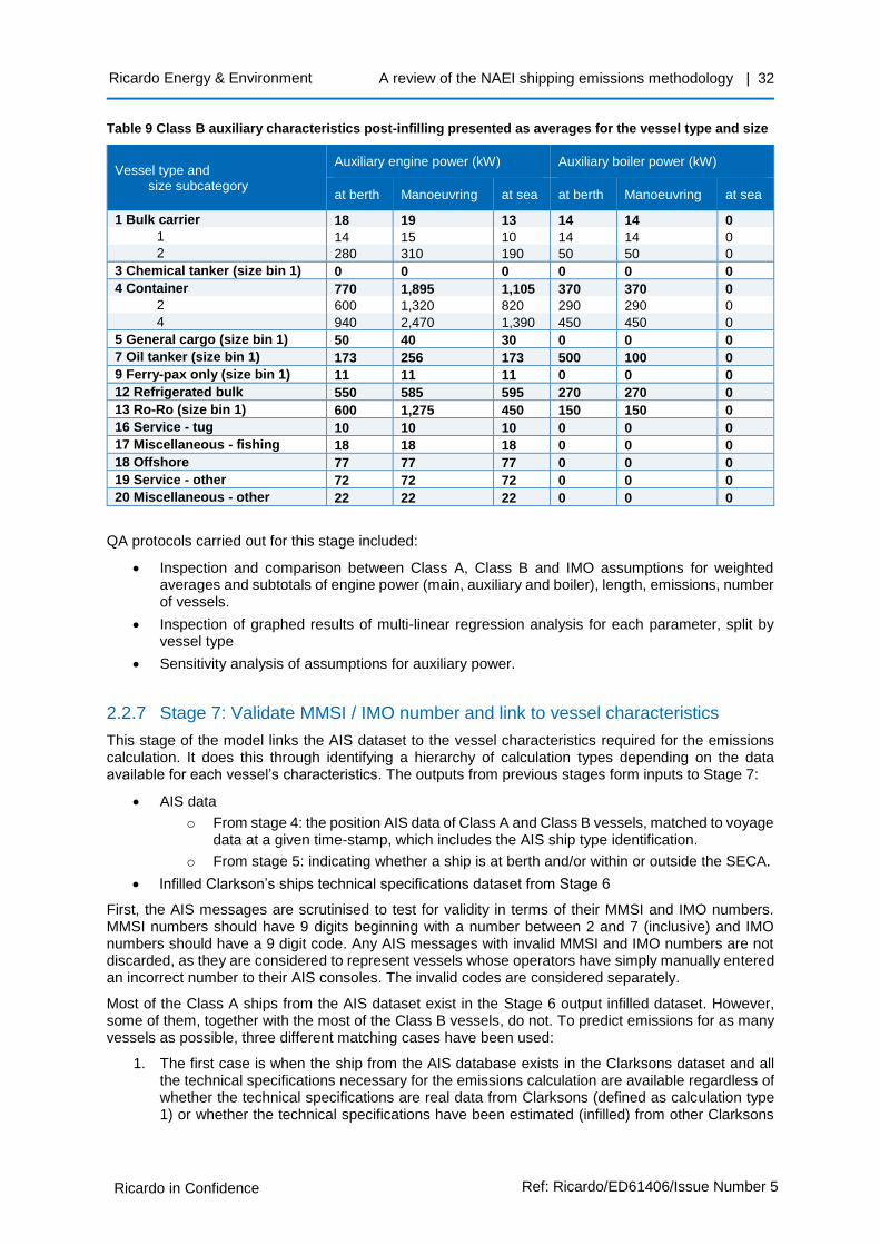
A review of the NAEI shipping emissions methodology | 32
Ricardo in Confidence Ref: Ricardo/ED61406/Issue Number 5
Ricardo Energy & Environment
Table 9 Class B auxiliary characteristics post-infilling presented as averages for the vessel type and size
Vessel type and size subcategory
Auxiliary engine power (kW) Auxiliary boiler power (kW)
at berth Manoeuvring at sea at berth Manoeuvring at sea
1 Bulk carrier 18 19 13 14 14 0
1 14 15 10 14 14 0
2 280 310 190 50 50 0
3 Chemical tanker (size bin 1) 0 0 0 0 0 0
4 Container 770 1,895 1,105 370 370 0
2 600 1,320 820 290 290 0
4 940 2,470 1,390 450 450 0
5 General cargo (size bin 1) 50 40 30 0 0 0
7 Oil tanker (size bin 1) 173 256 173 500 100 0
9 Ferry-pax only (size bin 1) 11 11 11 0 0 0
12 Refrigerated bulk 550 585 595 270 270 0
13 Ro-Ro (size bin 1) 600 1,275 450 150 150 0
16 Service - tug 10 10 10 0 0 0
17 Miscellaneous - fishing 18 18 18 0 0 0
18 Offshore 77 77 77 0 0 0
19 Service - other 72 72 72 0 0 0
20 Miscellaneous - other 22 22 22 0 0 0
QA protocols carried out for this stage included:
• Inspection and comparison between Class A, Class B and IMO assumptions for weighted averages and subtotals of engine power (main, auxiliary and boiler), length, emissions, number of vessels.
• Inspection of graphed results of multi-linear regression analysis for each parameter, split by vessel type
• Sensitivity analysis of assumptions for auxiliary power.
2.2.7 Stage 7: Validate MMSI / IMO number and link to vessel characteristics
This stage of the model links the AIS dataset to the vessel characteristics required for the emissions calculation. It does this through identifying a hierarchy of calculation types depending on the data available for each vessel’s characteristics. The outputs from previous stages form inputs to Stage 7:
• AIS data
o From stage 4: the position AIS data of Class A and Class B vessels, matched to voyage data at a given time-stamp, which includes the AIS ship type identification.
o From stage 5: indicating whether a ship is at berth and/or within or outside the SECA.
• Infilled Clarkson’s ships technical specifications dataset from Stage 6
First, the AIS messages are scrutinised to test for validity in terms of their MMSI and IMO numbers. MMSI numbers should have 9 digits beginning with a number between 2 and 7 (inclusive) and IMO numbers should have a 9 digit code. Any AIS messages with invalid MMSI and IMO numbers are not discarded, as they are considered to represent vessels whose operators have simply manually entered an incorrect number to their AIS consoles. The invalid codes are considered separately.
Most of the Class A ships from the AIS dataset exist in the Stage 6 output infilled dataset. However, some of them, together with the most of the Class B vessels, do not. To predict emissions for as many vessels as possible, three different matching cases have been used:
1. The first case is when the ship from the AIS database exists in the Clarksons dataset and all the technical specifications necessary for the emissions calculation are available regardless of whether the technical specifications are real data from Clarksons (defined as calculation type 1) or whether the technical specifications have been estimated (infilled) from other Clarksons

A review of the NAEI shipping emissions methodology | 33
Ricardo in Confidence Ref: Ricardo/ED61406/Issue Number 5
Ricardo Energy & Environment
data in Stage 6 (defined as calculation type 2). These technical data include length, beam, draught, deadweight, main engine power and ship design speed with allocated ship type bin. The ship matching process is based on the MMSI number if the MMSI number is unique in the vessels database and on the IMO number if the MMSI number is not unique.
2. The second case is when the ship from the AIS database exists in the Clarksons dataset but some missing technical specifications could not be infilled from Clarksons data but could instead be infilled using the infilling algorithm in Stage 6 using vessels design length, beam and ship type reported in the AIS data. Depending on the available data as well as its quality, calculations performed under this case are flagged with the calculation types 3, 4, 5 or 6.
3. The third case is when the ship was not found in the Clarksons dataset. This includes if the MMSI or IMO number was invalid. In this case all the technical data are infilled with the same infilling algorithm expressed in Stage 6, except that ship beam, length and AIS type bin are taken from the AIS message. The matching assumptions are based on the ship type reported in the AIS message, which was mapped to the IMO ship types used in the model.
The relevant regression formulae for predicting the missing speed, power, deadweight and/or draught are created based on the lengths and beams from the infilled Clarksons database for the relevant ship type. Then using these resultant formulae, the missing technical specifications are infilled based on the AIS beam and length provided. In some cases, however, the AIS length, beam and/or AIS ships types have errors. For such instances, the assumptions flagged as calculation types 4, 5, 6 or 7 were created. All calculation types are defined in Table 10.
Table 10 Descriptions of the calculation type indicators. There is higher uncertainty in the emission estimates for calculation types 3, 4, 5, 6 and 7.
Calculation type
Description and assumptions
Calculation Type 1
The ship and all required technical specifications exist in the vessel characteristics database without any in-filling.
Calculation Type 2
The ship is listed in the vessel characteristics database, and the missing technical specifications were infilled in Stage 6.
Calculation Type 3
The ship is either not listed in the vessel characteristics dataset or its missing technical specifications could not be infilled from other vessel characteristics data due to missing data. The missing data points were instead infilled with the infilling algorithm using data from the AIS messages of vessel length and beam, where the length and beam were deemed correct.
Calculation Type 4
The ship is either not listed in the vessel characteristics dataset or its missing technical specifications could not be infilled from other vessel characteristics data due to missing data. The missing data points were instead infilled with the infilling algorithm using data from the AIS messages of vessel length, and the vessel beam reported by AIS data was deemed erroneous or missing and instead assumed to be ¼ of AIS Length.
Calculation Type 5
The ship is either not listed in the vessel characteristics dataset or its missing technical specifications could not be infilled from other vessel characteristics data due to missing data. The AIS reported length and beam were either missing or deemed erroneous. The missing data points were instead infilled with the infilling algorithm using the median Length and Beam for the particular ship type/size category. The median values were pre-estimated based on calculation types 1-4 separately for class A and B.
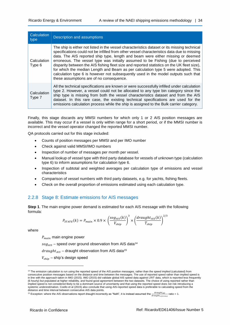
A review of the NAEI shipping emissions methodology | 34
Ricardo in Confidence Ref: Ricardo/ED61406/Issue Number 5
Ricardo Energy & Environment
Calculation type
Description and assumptions
Calculation Type 6
The ship is either not listed in the vessel characteristics dataset or its missing technical specifications could not be infilled from other vessel characteristics data due to missing data. The AIS reported ship type, length and beam were either missing or deemed erroneous. The vessel type was initially assumed to be Fishing (due to perceived disparity between the AIS fishing fleet size and reported statistics on the UK fleet size), for which the median Length and Beam as per calculation type 5 were adopted. This calculation type 6 is however not subsequently used in the model outputs such that these assumptions are of no consequence.
Calculation Type 7
All the technical specifications are known or were successfully infilled under calculation type 2. However, a vessel could not be allocated to any type bin category since the ship type is missing from both the vessel characteristics dataset and from the AIS dataset. In this rare case, the existing technical specifications are used for the emissions calculation process while the ship is assigned to the Bulk carrier category.
Finally, this stage discards any MMSI numbers for which only 1 or 2 AIS position messages are available. This may occur if a vessel is only within range for a short period, or if the MMSI number is incorrect and the vessel operator changed the reported MMSI number.
QA protocols carried out for this stage included:
• Counts of position messages per MMSI and per IMO number
• Check against valid MMSI/IMO numbers
• Inspection of number of messages per month per vessel.
• Manual lookup of vessel type with third party database for vessels of unknown type (calculation type 6) to inform assumptions for calculation type 6.
• Inspection of subtotal and weighted averages per calculation type of emissions and vessel characteristics
• Comparison of vessel numbers with third party datasets, e.g. for yachts, fishing fleets.
• Check on the overall proportion of emissions estimated using each calculation type.
2.2.8 Stage 8: Estimate emissions for AIS messages
Step 1. The main engine power demand is estimated for each AIS message with the following
formula:
𝑃𝑆𝑇𝐴𝑇𝐸(𝑘) = 𝑃𝑚𝑎𝑖𝑛 × 0.9 × (𝑠𝑜𝑔𝐴𝐼𝑆(𝑘)
𝑉𝑠ℎ𝑖𝑝
)
3
× (𝑑𝑟𝑎𝑢𝑔ℎ𝑡𝐴𝐼𝑆(𝑘)
𝑇𝑠ℎ𝑖𝑝
)
2/3
where
𝑃𝑚𝑎𝑖𝑛 main engine power
𝑠𝑜𝑔𝐴𝐼𝑆 – speed over ground observation from AIS data14
𝑑𝑟𝑎𝑢𝑔ℎ𝑡𝐴𝐼𝑆 – draught observation from AIS data15
𝑉𝑠ℎ𝑖𝑝 – ship’s design speed
14 The emission calculation is run using the reported speed of the AIS position messages, rather than the speed implied (calculated) from consecutive position messages based on the distance and time between the messages. The use of reported speed rather than implied speed is in line with the approach taken in IMO (2015). IMO (2015) did validate global AIS speed data against LRIT data, which is reported less frequently (6 hourly) but populated at higher reliability, and found good agreement between the two datasets. The choice of using reported rather than implied speed is not considered likely to be a dominant source of uncertainty and that using the reported speed does not risk introducing a systemic underestimation. Coello et al (2015) also conclude that using AIS-reported speed data is preferable to calculating speed from the distance and time interval between consecutive AIS data points. 15 Exception: where the AIS observations report draught incorrectly as “NaN”, it is instead assumed the
𝑑𝑟𝑎𝑢𝑔ℎ𝑡𝐴𝐼𝑆
𝑑𝑟𝑎𝑢𝑔ℎ𝑡𝑟𝑒𝑓𝑒𝑟𝑒𝑛𝑐𝑒 ratio = 1.

A review of the NAEI shipping emissions methodology | 35
Ricardo in Confidence Ref: Ricardo/ED61406/Issue Number 5
Ricardo Energy & Environment
𝑇𝑠ℎ𝑖𝑝 – ship’s design draught
k – number of observations.
Step 2. The instantaneous main engine load is calculated for each AIS message as:
𝐿𝑂𝐴𝐷𝑆𝑇𝐴𝑇𝐸(𝑘) =𝑃𝑆𝑇𝐴𝑇𝐸(𝑘)
𝑃𝑚𝑎𝑖𝑛
Power demands for auxiliary engines and boilers were set out in section 2.2.5, with load factors of 50% for both in all cases.
Step 3. The fuel type used is estimated. The following fuel types are distinguished in the 2014 base year inventory: heavy fuel oil (HFO, also residual oil) and marine diesel oil (MDO). LNG is assumed to not be used in the base year 2014 inventory, based on expert judgement indicating current (in 2014) use is negligible. Similarly, IMO (2015) assumes in its bottom-up estimates that LNG is not used in 2012 for domestic navigation or fishing.
Assumptions have been made of the types of fuel used in vessels, separately for main engines and the auxiliary engines and boilers. The assumptions have been based on judgement by the authors and aligned with IMO (2015). Outside of SECAs, the main engine fuel type is assumed to be HFO for vessels with main engine power greater than 3300kW or, where the engine speed is known for class A AIS messages, for vessels with slow and medium speed engines (less than 900rpm). Main engine fuel type is assumed to be MDO in other cases. If the main engine is assumed to run on MDO, then the auxiliaries are assumed to as well.16 Otherwise the fuel type for auxiliary engines and boilers is taken from IMO (2015) which stipulates the fuel type assumptions by vessel category and size.
Step 4. The fuel consumption and emissions (grams) are estimated for each AIS message using the following formulae:
𝐹𝐶(𝑘) = 𝑠𝑐𝑎𝑙𝑒_𝑓𝑎𝑐𝑡𝑜𝑟(𝑘) ∗ 𝑆𝐹𝑂𝐶 ∗ 𝐹𝐶𝑓𝑎𝑐𝑡𝑜𝑟 ∗ 𝑃𝑜𝑤𝑒𝑟(𝑘)
Where
𝑠𝑐𝑎𝑙𝑒_𝑓𝑎𝑐𝑡𝑜𝑟 (in hours) is the multiplier based on the time period between two AIS position messages to account for this time period, i.e. the calculation explicitly estimates emissions for the entire time period from one position message until the subsequent position message however long that time gap is.
SFOC (in g/kWh) is the engine fuel consumption taken from Table 11 or Table 12 depending on the engine’s type.
𝐹𝐶_𝑓𝑎𝑐𝑡𝑜𝑟 is the unitless fuel consumption factor calculated in accordance with the fuel type and current load (see Equation 1). This can also be referred as load adjustment factor applied to each instantaneous engine load.
Power (in kW) of the engine.
And
𝑃𝑜𝑙𝑙𝑢𝑡𝑎𝑛𝑡(𝑘) = 𝐹𝐶(𝑘) ∗ 𝐸𝐹
Where
𝐸𝐹 is the emission factor for one of the pollutants and described in the following subsections.
QA protocols carried out for this stage included:
• Derivation of implied sulphur content from SO2 emissions and fuel consumption
• Fuel types split by vessel type and SECA/non-SECA
• Check ratios of pollutants compared to existing NAEI
• Manual derivation of a calculation to re-produce model code results.
16 This additional assumption has been developed beyond the assumptions set out in IMO (2015) in order to generate suitable assumptions for class B vessels which are not considered in IMO (2015).
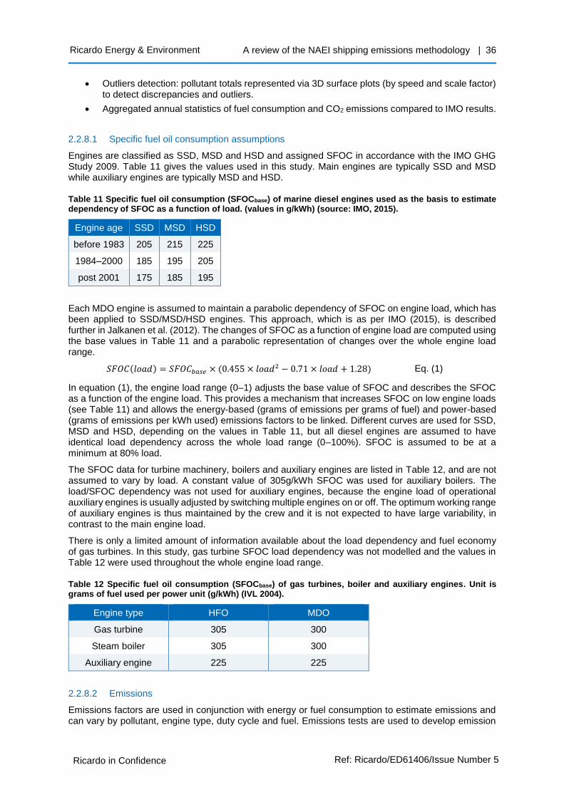
A review of the NAEI shipping emissions methodology | 36
Ricardo in Confidence Ref: Ricardo/ED61406/Issue Number 5
Ricardo Energy & Environment
• Outliers detection: pollutant totals represented via 3D surface plots (by speed and scale factor) to detect discrepancies and outliers.
• Aggregated annual statistics of fuel consumption and CO2 emissions compared to IMO results.
2.2.8.1 Specific fuel oil consumption assumptions
Engines are classified as SSD, MSD and HSD and assigned SFOC in accordance with the IMO GHG Study 2009. Table 11 gives the values used in this study. Main engines are typically SSD and MSD while auxiliary engines are typically MSD and HSD.
Table 11 Specific fuel oil consumption (SFOCbase) of marine diesel engines used as the basis to estimate dependency of SFOC as a function of load. (values in g/kWh) (source: IMO, 2015).
Engine age SSD MSD HSD
before 1983 205 215 225
1984–2000 185 195 205
post 2001 175 185 195
Each MDO engine is assumed to maintain a parabolic dependency of SFOC on engine load, which has been applied to SSD/MSD/HSD engines. This approach, which is as per IMO (2015), is described further in Jalkanen et al. (2012). The changes of SFOC as a function of engine load are computed using the base values in Table 11 and a parabolic representation of changes over the whole engine load range.
𝑆𝐹𝑂𝐶(𝑙𝑜𝑎𝑑) = 𝑆𝐹𝑂𝐶𝑏𝑎𝑠𝑒 × (0.455 × 𝑙𝑜𝑎𝑑2 − 0.71 × 𝑙𝑜𝑎𝑑 + 1.28) Eq. (1)
In equation (1), the engine load range (0–1) adjusts the base value of SFOC and describes the SFOC as a function of the engine load. This provides a mechanism that increases SFOC on low engine loads (see Table 11) and allows the energy-based (grams of emissions per grams of fuel) and power-based (grams of emissions per kWh used) emissions factors to be linked. Different curves are used for SSD, MSD and HSD, depending on the values in Table 11, but all diesel engines are assumed to have identical load dependency across the whole load range (0–100%). SFOC is assumed to be at a minimum at 80% load.
The SFOC data for turbine machinery, boilers and auxiliary engines are listed in Table 12, and are not assumed to vary by load. A constant value of 305g/kWh SFOC was used for auxiliary boilers. The load/SFOC dependency was not used for auxiliary engines, because the engine load of operational auxiliary engines is usually adjusted by switching multiple engines on or off. The optimum working range of auxiliary engines is thus maintained by the crew and it is not expected to have large variability, in contrast to the main engine load.
There is only a limited amount of information available about the load dependency and fuel economy of gas turbines. In this study, gas turbine SFOC load dependency was not modelled and the values in Table 12 were used throughout the whole engine load range.
Table 12 Specific fuel oil consumption (SFOCbase) of gas turbines, boiler and auxiliary engines. Unit is grams of fuel used per power unit (g/kWh) (IVL 2004).
Engine type HFO MDO
Gas turbine 305 300
Steam boiler 305 300
Auxiliary engine 225 225
2.2.8.2 Emissions
Emissions factors are used in conjunction with energy or fuel consumption to estimate emissions and can vary by pollutant, engine type, duty cycle and fuel. Emissions tests are used to develop emission

A review of the NAEI shipping emissions methodology | 37
Ricardo in Confidence Ref: Ricardo/ED61406/Issue Number 5
Ricardo Energy & Environment
factors in g/kWh and are converted to fuel-based emissions factors (grams pollutant per gram of fuel consumed) by dividing by the brake-specific fuel consumption (BSFC) or specific fuel oil consumption (SFOC) corresponding to the test associated with the emissions factors. Emissions factors vary by: engine type (main, auxiliary, auxiliary boilers); engine rating (slow speed diesel (SSD), medium speed diesel (MSD), high speed diesel (HSD)); whether engines are pre-IMO Tier I, or meet IMO Tier I or II requirements; and type of service (duty cycle) in which they operate (propulsion or auxiliary). Emissions factors are adjusted further for fuel type (HFO, MDO) and the sulphur content of the fuel being burned. Finally, engine load variability is incorporated into the factors used for estimating emissions.
All these variables were taken into account when estimating emissions in an approach identical to that taken in IMO (2015). Emissions factors were developed for the following GHGs and pollutants:
• carbon dioxide, CO2
• methane, CH4
• nitrous oxide, N2O
• non-methane volatile organic compounds, NMVOC
• oxides of nitrogen, NOx
• sulphur oxides, SOx
• particulate matter, PM
• carbon monoxide, CO
The following steps were taken:
Step 1. Identify baseline emissions factors. Emission factors come in two groups: energy-based in g pollutant/kWh and fuel-based in g pollutant/g fuel consumed. The baseline fuel for the bottom-up emission factors is defined as HFO fuel with 2.7% sulphur content (note: this is not the assumed fuel sulphur content – this is the baseline from which adjustments are made for the different fuel sulphur contents).
Step 2. Convert energy-based baseline emissions factors in g pollutant/kWh to fuel-based emission factors in pollutant/ g fuel consumed, as applicable, using:
𝐸𝐹𝑏𝑎𝑠𝑒𝑙𝑖𝑛𝑒 (𝑔 𝑝𝑜𝑙𝑙𝑢𝑡𝑎𝑛𝑡 𝑔 𝑓𝑢𝑒𝑙⁄ ) = 𝐸𝐹𝑏𝑎𝑠𝑒𝑙𝑖𝑛𝑒 (𝑔 𝑝𝑜𝑙𝑙𝑢𝑡𝑎𝑛𝑡 𝑘𝑊ℎ⁄ )
𝑆𝐹𝑂𝐶𝑏𝑎𝑠𝑒𝑙𝑖𝑛𝑒 (𝑔 𝑓𝑢𝑒𝑙 𝑘𝑊ℎ⁄ )
where,
EFbaseline – cited emission factor
SFOCbaseline – SFOC associated with the cited emission factor
Step 3. Use fuel correction factor (FCF), as applicable, to adjust emission factors for the specific fuel used by the engine.
𝐸𝐹𝑎𝑐𝑡𝑢𝑎𝑙 (𝑔 𝑝𝑜𝑙𝑙𝑢𝑡𝑎𝑛𝑡 𝑔 𝑓𝑢𝑒𝑙⁄ ) = 𝐸𝐹𝑏𝑎𝑠𝑒𝑙𝑖𝑛𝑒 (𝑔 𝑝𝑜𝑙𝑙𝑢𝑡𝑎𝑛𝑡 𝑔 𝑓𝑢𝑒𝑙⁄ ) × 𝐹𝐶𝐹
This is then converted to kg pollutant/tonne fuel consumed for the purposes of comparisons.
Step 4. Adjust EFactual based on variable engine loads using SFOC engine curves and low load adjustment factors to adjust the SFOC.
2.2.8.3 CO2 emission factors
The carbon content of each fuel type is constant and is not affected by engine type, duty cycle or other parameters when looking on a kg CO2 per tonne fuel basis. The fuel-based CO2 emissions factors for main and auxiliary engines at slow, medium and high speeds are the same as assumed in IMO (2015) and are based on MEPC 63/23, Annex 8:
HFO EFbaseline CO2 = 3,114 kg CO2/tonne fuel
MDO EFbaseline CO2 = 3,206 kg CO2/ tonne fuel
LNG EFbaseline CO2 = 2,750 kg CO2/ tonne fuel
The CO2 factors listed above differ from the factors currently used in the NAEI. They are 3.4% lower than in the NAEI for fuel oil and 0.5% higher than in the NAEI for gas oil. The differences are shown in Table 13. The differences are quite large for fuel oil, but the newly proposed figures are much closer to the defaults in the 2006 IPCC Guidelines than the existing values used in the current NAEI.

A review of the NAEI shipping emissions methodology | 38
Ricardo in Confidence Ref: Ricardo/ED61406/Issue Number 5
Ricardo Energy & Environment
Table 13 Carbon factors for HFO and MDO
ktC/Mt Existing carbon factors
used in GHGI Proposed new carbon factors (IMO, 2015)
IPCC 2006 CEF using IPCC NCV
Fuel oil/HFO 879 849 853
Gas oil/MDO 870 874 869
2.2.8.4 CH4 emission factors
Methane emission factors for diesel-fuelled engines, steam boilers and gas turbines are the same as used in IMO (2015), which are ultimately taken from IVL (2004), which states that CH4 emissions are approximately 2% the magnitude of VOC. Therefore, the CH4 EFbaseline is derived by multiplying the NMVOC EFbaseline by 2%.
Although no LNG is present in the base year inventory, CH4 emission factors are important to consider from potential future LNG fuelled ships. The emissions factor for LNG Otto-cycle engines is taken from IMO (2015) as 8.5g/kWh, which is itself derived from (MARINTEK 2010, 2014). The majority of LNG-powered engines are assumed to be Otto-cycle.
From these sources, the CH4 EFbaseline factors presented in Table 14 were used. CH4 emissions are unaffected by the sulphur content of the fuel burned, and are the same for HFO and distillates (MDO).
Table 14 CH4 emissions factors (IMO, 2015)
Engine speed / type
Fuel type Main engine emission factor (kg/tonne fuel)
Auxiliary engine emission factor (kg/tonne fuel)
Original source of EFs
SSD HFO/MDO 0.06 N/A IVL (2004)
MSD HFO/MDO 0.05 0.04 IVL (2004)
HSD HFO/MDO N/A 0.04 IVL (2004)
Otto LNG 51.2 51.2 MARINTEK (2010)
GT HFO/MDO 0.01 N/A IVL (2004)
STM HFO/MDO 0.01 N/A IVL (2004)
2.2.8.5 N2O emission factors
The N2O emission factors are taken from IMO (2015) and are shown in Table 15. The LNG N2O EF baseline was converted from g/mmBTU to g/kWh assuming 38% engine efficiency, and then converted to grams N2O per gram fuel using an SFOC of 166g fuel/kWh. N2O emission factors are unaffected by fuel sulphur content but do change slightly between HFO and distillate fuels. The emission factors for MDO are derived from those for HFO with the following correction factor: 𝐸𝐹𝑀𝐷𝑂 = 0.94 ∗ 𝐸𝐹𝐻𝐹𝑂.
Table 15 N2O baseline emissions factors (IMO, 2015)
Engine speed / type
Fuel type
Main engine emission factor (kg/tonne fuel)
Auxiliary engine emission factor (kg/tonne fuel)
Original source of EFs
SSD HFO 0.16 N/A USEPA (2014)
MSD HFO 0.16 0.16 USEPA (2014)
HSD HFO N/A 0.16 USEPA (2014)
Otto LNG 0.11 0.11 Kunz & Gorse (2013)
GT HFO 0.16 N/A USEPA (2014)
STM HFO 0.16 N/A USEPA (2014)

A review of the NAEI shipping emissions methodology | 39
Ricardo in Confidence Ref: Ricardo/ED61406/Issue Number 5
Ricardo Energy & Environment
2.2.8.6 NOx emission factors
The NOX emission factors are taken from IMO (2015). The NOx emission factors for main and auxiliary engines rated at slow, medium and high speeds were assigned according to Tier I and II standards as defined in MARPOL Annex VI, Regulation 13 for limiting the emissions of NOX. Emissions for Tier 0 engines (constructed before 2000) were modelled in accordance with Starcrest (2013). The SFOC corresponding to the energy-based emission factors was used to convert to fuel-based emissions factors. NOx EFbaseline for boilers (denoted by STM respectively in Table 16) remains the same, as there are no IMO emissions standards that apply to boiler emissions. The emission factors used in the study are presented in Table 16. NOx emissions are unaffected by fuel sulphur content but do change slightly between HFO and distillate fuels. The emission factors for MDO are derived from those for HFO with the following correction factor: 𝐸𝐹𝑀𝐷𝑂 = 0.94 ∗ 𝐸𝐹𝐻𝐹𝑂.
Table 16 NOx baseline emissions factors (IMO, 2015)
IMO Tier
Engine speed / type
Fuel type
Specific fuel oil consumption (SFOC) Main/Aux
Main engine EFbaseline (kg/tonne fuel)
Aux. engine EFbaseline (kg/tonne fuel)
Original source of EFs
0
SSD HFO 195 / NA 92.82 N/A
ENTEC (2002) MSD HFO 215 / 227 65.12 64.76
HSD HFO NA / 227 N/A 51.10
1
SSD HFO 195 / NA 87.18 N/A MARPOL Annex VI, Regulation 13 Tier I
MSD HFO 215 / 227 60.47 57.27
HSD HFO NA / 227 N/A 45.81
2
SSD HFO 195 / NA 78.46 N/A MARPOL Annex VI, Regulation 13 Tier II
MSD HFO 215 / 227 52.09 49.34
HSD MDO NA / 227 N/A 36.12
All Otto LNG 166 7.83 7.83 Kristensen (2012)
NA GT HFO 305 20.00 N/A IVL (2004)
NA STM HFO 305 6.89 N/A IVL (2004)
Notes: GT – gas turbine; STM – steam boiler
Fuel consumption efficiency improvements associated with Tier I and II engines is taken into account and further explained in the SFOC variability with load section 2.2.8.1.
2.2.8.7 SOx emission factors
For all three ship emissions sources, SOx emissions are directly linked to the sulphur content of the fuel consumed. More than 97% of the fuel sulphur is emitted as SOx and the convention in emission inventories is to report SOx emissions as SO2 equivalent17. Assuming all sulphur is released as SOx, the amount of SOx emissions is simply twice the amount of sulphur consumed in the fuel. So a 1% S-containing fuel yields 20 g SOx per kg fuel consumed.
The sulphur content of fuel used by vessels in UK waters has varied over the years for different fuel types and according to current sulphur emission control regulations. The SOx factors are therefore year dependent, fuel-type dependent and sea territory- and operation-dependent (i.e. whether inside or outside a SECA, at berth). The SOx factors for RFO and MDO, in different sea areas and at berth for 2014 and for other years back to 1990 and forward to 2030 are discussed further in Section 3.
For LNG, a factor of 0.02 gSO2/kg fuel is used taken from IMO (2015).
17 Note that some small amount of sulphur is locked up in particulate matter emissions, but given the level of uncertainty on the sulphur contents of fuels used by UK domestic shipping, this level of detail has not been considered.
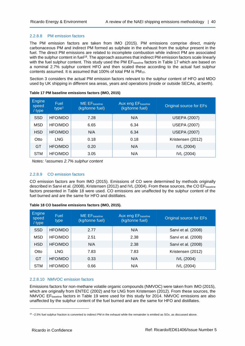
A review of the NAEI shipping emissions methodology | 40
Ricardo in Confidence Ref: Ricardo/ED61406/Issue Number 5
Ricardo Energy & Environment
2.2.8.8 PM emission factors
The PM emission factors are taken from IMO (2015). PM emissions comprise direct, mainly carbonaceous PM and indirect PM formed as sulphate in the exhaust from the sulphur present in the fuel. The direct PM emissions are related to incomplete combustion while indirect PM are associated with the sulphur content in fuel18. The approach assumes that indirect PM emission factors scale linearly with the fuel sulphur content. This study used the PM EFbaseline factors in Table 17 which are based on a nominal 2.7% sulphur content HFO and then scaled these according to the actual fuel sulphur contents assumed. It is assumed that 100% of total PM is PM10.
Section 3 considers the actual PM emission factors relevant to the sulphur content of HFO and MDO used by UK shipping in different sea areas, years and operations (inside or outside SECAs, at berth).
Table 17 PM baseline emissions factors (IMO, 2015)
Engine speed / type
Fuel type1
ME EFbaseline
(kg/tonne fuel) Aux eng EFbaseline
(kg/tonne fuel) Original source for EFs
SSD HFO/MDO 7.28 N/A USEPA (2007)
MSD HFO/MDO 6.65 6.34 USEPA (2007)
HSD HFO/MDO N/A 6.34 USEPA (2007)
Otto LNG 0.18 0.18 Kristensen (2012)
GT HFO/MDO 0.20 N/A IVL (2004)
STM HFO/MDO 3.05 N/A IVL (2004)
Notes: 1assumes 2.7% sulphur content
2.2.8.9 CO emission factors
CO emission factors are from IMO (2015). Emissions of CO were determined by methods originally described in Sarvi et al. (2008), Kristensen (2012) and IVL (2004). From these sources, the CO EFbaseline factors presented in Table 18 were used. CO emissions are unaffected by the sulphur content of the fuel burned and are the same for HFO and distillates.
Table 18 CO baseline emissions factors (IMO, 2015).
Engine speed / type
Fuel type
ME EFbaseline
(kg/tonne fuel) Aux eng EFbaseline
(kg/tonne fuel) Original source for EFs
SSD HFO/MDO 2.77 N/A Sarvi et al. (2008)
MSD HFO/MDO 2.51 2.38 Sarvi et al. (2008)
HSD HFO/MDO N/A 2.38 Sarvi et al. (2008)
Otto LNG 7.83 7.83 Kristensen (2012)
GT HFO/MDO 0.33 N/A IVL (2004)
STM HFO/MDO 0.66 N/A IVL (2004)
2.2.8.10 NMVOC emission factors
Emissions factors for non-methane volatile organic compounds (NMVOC) were taken from IMO (2015), which are originally from ENTEC (2002) and for LNG from Kristensen (2012). From these sources, the NMVOC EFbaseline factors in Table 19 were used for this study for 2014. NMVOC emissions are also unaffected by the sulphur content of the fuel burned and are the same for HFO and distillates.
18 ~2.5% fuel sulphur fraction is converted to indirect PM in the exhaust while the remainder is emitted as SOx, as discussed above.

A review of the NAEI shipping emissions methodology | 41
Ricardo in Confidence Ref: Ricardo/ED61406/Issue Number 5
Ricardo Energy & Environment
Table 19: NMVOC baseline emissions factors (IMO, 2015)
Engine speed / type
Fuel type
ME EFbaseline
(kg/tonne fuel) Aux eng EFbaseline
(kg/tonne fuel) Original source for EFs
SSD HFO/MDO 3.08 n/a ENTEC (2002)
MSD HFO/MDO 2.33 1.76 ENTEC (2002)
HSD HFO/MDO n/a 1.76 ENTEC (2002)
Otto LNG 3.01 3.01 Kristensen (2012)
GT HFO/MDO 0.33 n/a ENTEC (2002)
STM HFO/MDO 0.33 n/a ENTEC (2002)
2.2.9 Stage 9: Assign AIS message as UK domestic, UK international, crown dependency or passing movement
The previous Entec (2010) methodology relied on the use of a database of vessel movements from port to port. This methodology made it straightforward to allocate emissions to the UK or not. However, using such databases for inventory purposes has limitations of: potential under-reporting of vessel movements; and no capture of vessel routes, speeds and intermediate stops at anchorages. Conversely, using AIS data requires additional processing to identify how each position message is part of a vessel’s voyage, and then process how to allocate that voyage.
Existing work carried out in MMO (2014) developed a tool for the processing of raw AIS data from the MCA, which included the classification of movements as UK domestic, UK international or transits. This classification relied on assumptions regarding when a vessel called at a UK port, which was taken as if the vessel position came within 0.5nm of the UK coastline, or of a port (MMO, 2013). However, inspection of the results of the tool in MMO (2014) highlighted imperfect allocation between UK domestic and UK international movements as there were movements shown between the UK and neighbouring countries marked as domestic. Furthermore, the MMO tool was set up to use input data in weekly batches. But splitting data into weekly batches leads to many voyages split across separate batches, and as such the start or end points of these voyages are not both known and thus these voyages cannot be classified as domestic or international without introducing a lot of uncertainty.
To improve on this, a whole year’s worth of AIS data were processed together rather than separate batches of weeks of data. Furthermore, given the need to provide additional breakdown for inventory purposes of isolating activity related to Crown Dependencies a new algorithm has been developed which allocates AIS position messages as related to one of UK domestic, UK international, Crown Dependencies or transit (not calling at the UK or Crown dependencies). A descriptive summary of the steps in Stage 9 of the model is given in Table 20 and a table showing all the combinations of vessel and movement types and how these are allocated is summarised as Table 21.
Table 20 Description of method used to assign AIS message as UK domestic, UK international, crown dependency or passing movement
Step Description
1 Identify consecutive AIS position messages from the same MMSI number as part of a voyage.
2
Define territory geographical areas for the UK, Crown Dependencies and international destinations. A combination of datasets has been used to determine these territory locations such as the ports and administrative boundaries for the UK, and the Country defined European coast line boundaries for the rest. A 5-km buffer zone on the European coast line boundaries has been used, assuming that in the case a vessel is shown within 5 km from an international coast, then its destination is international, with the exception of the narrowest part of the Dover Strait and the boundary between Ireland and Northern Ireland (Figure 14).
3 Allocate each AIS position message to a territory, when this message is located within a territory geographical area as defined above. This suggests that the vessel is deemed to have stopped at the country to this destination.

A review of the NAEI shipping emissions methodology | 42
Ricardo in Confidence Ref: Ricardo/ED61406/Issue Number 5
Ricardo Energy & Environment
Step Description
4
Allocate the non-defined position messages (AIS position messages in between messages with allocated territory information as described on the previous step) to a specific trip type movement. This was expressed according to the origin and destination of the consecutive AIS position messages from the same MMSI number:
• from the UK to the UK the voyage is defined as UK domestic
• from the UK to a Crown Dependency – defined as Domestic Crown Dependency; from a Crown Dependency to the UK or another Crown Dependency – defined as Crown Dependency (the results in this report combine both as ‘Crown Dependencies’)
• From the UK to another country the voyage is defined as UK international
• From another country to the UK the voyage is defined as UK international
• Not calling at the UK or a Crown Dependency the voyage is defined as transit voyage
5 The time vessel spent in port at berth is conservatively classed as UK domestic if it has been located in the UK, regardless of where the vessel previously travelled from or where it next travelled to.
6
Reallocation to UK international of trip movements where:
• there is a 24-hour temporal gap during a ‘passage’ AND
• the vessel category is cargo or passenger (i.e. not fishing, offshore, service or miscellaneous vessels).
Generate ‘passages’ which define voyages based on sequences of AIS position messages using vessel’s start and stop status (being stationary for more than 5 minutes). All the activity of the AIS position messages from these passages is redefined as UK international.
7
Additional reallocation of trip type movement on the UK domestic position messages where a vessel has stopped within 500 metres from a non-UK offshore destination.19 Further information on what constitutes an offshore location is in section 2.4.9. All the activity of the AIS position messages from these passages is redefined as UK international.
Table 21 Summary of allocation assumptions (CD: Crown dependencies)
Vessel type Depart Gaps between AIS messages
Arrive Allocation
Fishing, Offshore, Service-tug, Service-other, Miscellaneous
Leave UK coast Any Arrive UK coast Domestic
Cargo, passenger
Leave UK coast Gap <24 hours Arrive UK coast Domestic
All Leave UK / CD coast Any Arrive CD coast CD
All Leave UK coast Any Arrive non-UK coast UK international
All Leave non-UK coast Any Arrive UK coast UK international*
Cargo, passenger
Leave UK coast Gap >24 hours Arrive UK coast UK international
All Neither UK nor CD Any Neither UK nor CD Transit
*The existing NAEI reporting of international shipping as a memo item effectively excludes this line, as the international bunker sales relates only to outbound voyages
19 Reference: http://www.cesma-eu.org/MSP.pdf
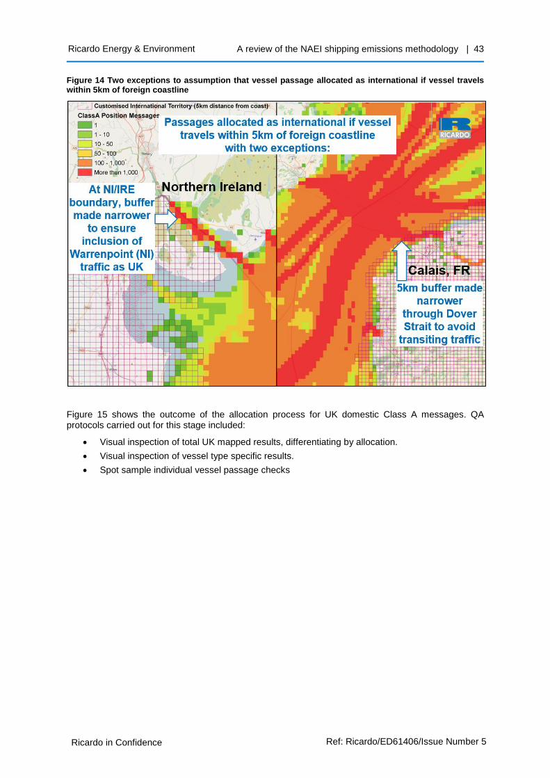
A review of the NAEI shipping emissions methodology | 43
Ricardo in Confidence Ref: Ricardo/ED61406/Issue Number 5
Ricardo Energy & Environment
Figure 14 Two exceptions to assumption that vessel passage allocated as international if vessel travels within 5km of foreign coastline
Figure 15 shows the outcome of the allocation process for UK domestic Class A messages. QA protocols carried out for this stage included:
• Visual inspection of total UK mapped results, differentiating by allocation.
• Visual inspection of vessel type specific results.
• Spot sample individual vessel passage checks

A review of the NAEI shipping emissions methodology | 44
Ricardo in Confidence Ref: Ricardo/ED61406/Issue Number 5
Ricardo Energy & Environment
Figure 15 AIS Class A position messages (per km2) in 2014 allocated as domestic
2.2.10 Stage 10: Compile base year inventory
The final stage of the model assembles the shipping emissions estimates. Specifically this includes:
• Combining Class A and Class B estimates.
• Removing fuel consumption and emission estimates from vessels estimated to be at berth for more than 24 hours, as it is judged that if the vessel is stationary at berth for more than this period they are likely to be laid up and not running auxiliary engines or boilers.20
20 Expert judgement of the project team.

A review of the NAEI shipping emissions methodology | 45
Ricardo in Confidence Ref: Ricardo/ED61406/Issue Number 5
Ricardo Energy & Environment
• Removing AIS-based estimates for vessels which are of unknown type (described in section 2.4.6).
• Removing the AIS-based estimates for category 15 Yachts. These will instead be covered in the NAEI with existing estimates in category ‘inland waterways’ from AEA (2011) for:
o 01. Sailing boats with auxiliary engines
o 02. Motorboats – inland waterways
o 02. Motorboats – coastal excluding Coastal Passenger vessels >12 passengers
A more detailed discussion on the exclusion of category yachts is in section 2.4.7.
The new AIS-based model includes estimates for some categories of vessel that would lead to double counting of certain components that are currently included in the NAEI under inland waterways. The reason for this overlap is that the NAEI had aimed to capture those smaller vessels, mainly operating in river estuaries and recreational boats that did not go far out to sea, because they had not been captured in the original Entec (2010) shipping study. The overlap with the current NAEI inventory for inland waterways is being considered for the next compilation of the inventory to be submitted in 2018. This exercise will aim to remove those vessel activities now captured in the new shipping inventory estimates from the NAEI’s separate inland waterways emissions inventory to avoid this double-count. The expectation is that at least the following changes will need to be made:
• AIS-based estimates for category 16 Service-Tugs will replace the existing estimates in ‘inland waterways’ for Workboats – Tug.
• AIS-based estimates for category 17 Miscellaneous-Fishing will replace the existing estimates in ‘inland waterways’ for Workboats – fishing and commercial fishing vessels.
• AIS-based estimates for category 19 Service-Other will replace the existing estimates in ‘inland waterways’ for Workboats – crane >12m.
QA protocols carried out for this stage included:
• Comparison against existing NAEI estimates, split by vessel type
• Validation against existing literature for North Sea and English Channel.
2.3 Results
2.3.1 Fuel consumption
The estimates of fuel consumption for Class A and Class B vessels are shown for HFO in Table 22 and for MDO in Table 23. The estimates are split according to whether they are classed as domestic, crown dependencies, UK international, or non-UK movement (‘transit’), and are further split by at berth or at sea, with the at sea portion separately estimated for those position messages with gaps of more than 24 hours between messages.
Table 22 and Table 23 show that, for the UK domestic and crown dependencies total in 2014, estimates for MDO dominate those of HFO. This trend will shift further in favour of MDO for year 2015, due to the assumptions applied for compliance with the MARPOL Annex VI sulphur limits in SECAs in force from 2015. Fuel consumption from AIS Class B reporting vessels is assumed to be almost exclusively MDO.
The UK domestic total is small compared to the total estimates for UK international and transit voyages. The figures for UK international and transit are not just those estimated to occur in UK waters, but also include fuel consumption as estimated by the model to cover the period until the next position message for a MMSI number is received (i.e. will overestimate fuel consumption if vessels outside of UK terrestrial AIS range stop in a foreign port).
Roughly one sixth of the total fuel consumption is attributed to the position messages which precede long (>24 hour) gaps before subsequent messages for the same vessel MMSI (listed in tables as “At sea, AIS message gap >24 hrs”). This gap is most likely when a vessel leaves the terrestrial AIS coverage. Based on the assumptions applied, the fuel and emissions covering the entire time gap until the next position message has been calculated and is allocated as UK domestic for fishing, service and offshore industry vessels, if the vessel previously and subsequently calls at the UK. There is higher uncertainty in the accuracy and allocation of this component compared to other estimates (for vessels other than fishing, this is 11% of UK domestic total fuel consumption) since the vessel during the gap

A review of the NAEI shipping emissions methodology | 46
Ricardo in Confidence Ref: Ricardo/ED61406/Issue Number 5
Ricardo Energy & Environment
in AIS coverage may not have continued sailing at the same speed during the entire gap in position messages, and may have visited another country. For fishing vessels, this component (18 kt HFO and 92kt MDO) makes up 55% of total fishing fuel consumption, which is further discussed in section 2.4.5.
Table 22 Total HFO consumption in 2014 split by at berth/sea and by allocation (kt)
Vessel category
At berth / at sea UK domestic (kt)
Crown dependencies (kt)
UK international (kt)
Transit (kt)
All except fishing
At berth <24 hours 0 0 0 0
At sea, AIS message gaps <24 hrs 465 3 2,569 4,627
At sea, AIS message gap >24 hrs 28 0 11,735 15,029
Subtotal 493 3 14,304 19,656
Fishing
At berth <24 hours 0 0 0 0
At sea, AIS message gaps <24 hrs 6 0 4 59
At sea, AIS message gap >24 hrs 18 0 8 159
Subtotal 24 0 12 219
Total Total 517 3 14,316 19,875
Table 23 Total MDO consumption in 2014 split by at berth/sea and by allocation (kt)
Vessel category
At berth / at sea UK domestic (kt)
Crown dependencies (kt)
UK international (kt)
Transit (kt)
All except fishing
At berth <24 hours 143 1.0 16 55
At sea, AIS message gaps <24 hrs 600 12 796 2,508
At sea, AIS message gap >24 hrs 122 0.2 2,824 3,325
Subtotal 865 13 3,636 5,888
Fishing
At berth <24 hours 9 0.2 0.1 11
At sea, AIS message gaps <24 hrs 72 1.1 13 272
At sea, AIS message gap >24 hrs 92 1.8 17 305
Subtotal 174 3.1 30 588
Total Total 1,039 17 3,666 6,476
The split in the estimated fuel consumption between main engines, auxiliary engines and auxiliary boilers is shown in Table 24 for all vessel types. This shows that, on average across the vessel types, the fuel consumption estimated from main engines as a proportion of the total fuel consumption is 79%, varying from 46% to 87%. This result is lower than the IPCC 2006 GL which suggests that over 95% of fuel consumption results from main engines. The result is however higher than the more recent IMO (2015) inventory, which is also AIS based, which estimated around 70% of fuel consumption is from main engines.21 Importantly, IMO (2015) acknowledge that estimates for auxiliary engines “will remain an area of significant assumption for the foreseeable future”, i.e. in the absence of data, estimates of auxiliary engines’ fuel consumption are heavily reliant on assumptions. This model estimates in this regard are therefore between the IPCC 2006 GL and IMO (2015).
21 Extracted from IMO (2015) Figure 28.
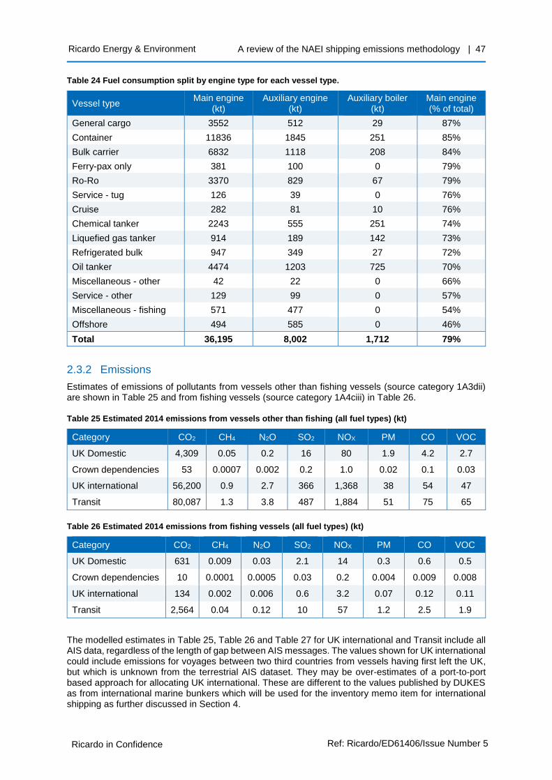
A review of the NAEI shipping emissions methodology | 47
Ricardo in Confidence Ref: Ricardo/ED61406/Issue Number 5
Ricardo Energy & Environment
Table 24 Fuel consumption split by engine type for each vessel type.
Vessel type Main engine
(kt) Auxiliary engine
(kt) Auxiliary boiler
(kt) Main engine (% of total)
General cargo 3552 512 29 87%
Container 11836 1845 251 85%
Bulk carrier 6832 1118 208 84%
Ferry-pax only 381 100 0 79%
Ro-Ro 3370 829 67 79%
Service - tug 126 39 0 76%
Cruise 282 81 10 76%
Chemical tanker 2243 555 251 74%
Liquefied gas tanker 914 189 142 73%
Refrigerated bulk 947 349 27 72%
Oil tanker 4474 1203 725 70%
Miscellaneous - other 42 22 0 66%
Service - other 129 99 0 57%
Miscellaneous - fishing 571 477 0 54%
Offshore 494 585 0 46%
Total 36,195 8,002 1,712 79%
2.3.2 Emissions
Estimates of emissions of pollutants from vessels other than fishing vessels (source category 1A3dii) are shown in Table 25 and from fishing vessels (source category 1A4ciii) in Table 26.
Table 25 Estimated 2014 emissions from vessels other than fishing (all fuel types) (kt)
Category CO2 CH4 N2O SO2 NOX PM CO VOC
UK Domestic 4,309 0.05 0.2 16 80 1.9 4.2 2.7
Crown dependencies 53 0.0007 0.002 0.2 1.0 0.02 0.1 0.03
UK international 56,200 0.9 2.7 366 1,368 38 54 47
Transit 80,087 1.3 3.8 487 1,884 51 75 65
Table 26 Estimated 2014 emissions from fishing vessels (all fuel types) (kt)
Category CO2 CH4 N2O SO2 NOX PM CO VOC
UK Domestic 631 0.009 0.03 2.1 14 0.3 0.6 0.5
Crown dependencies 10 0.0001 0.0005 0.03 0.2 0.004 0.009 0.008
UK international 134 0.002 0.006 0.6 3.2 0.07 0.12 0.11
Transit 2,564 0.04 0.12 10 57 1.2 2.5 1.9
The modelled estimates in Table 25, Table 26 and Table 27 for UK international and Transit include all AIS data, regardless of the length of gap between AIS messages. The values shown for UK international could include emissions for voyages between two third countries from vessels having first left the UK, but which is unknown from the terrestrial AIS dataset. They may be over-estimates of a port-to-port based approach for allocating UK international. These are different to the values published by DUKES as from international marine bunkers which will be used for the inventory memo item for international shipping as further discussed in Section 4.

A review of the NAEI shipping emissions methodology | 48
Ricardo in Confidence Ref: Ricardo/ED61406/Issue Number 5
Ricardo Energy & Environment
The total CO2 emissions for domestic and crown dependencies split by Class A and Class B, and by vessel type are shown in Figure 16. The figure shows that the majority of the total emissions are from (large) vessels reporting under Class A AIS; the emissions from (smaller) Class B vessels are estimated to make up approximately 6% of the total. Of this figure, fishing vessels make up source category 1A4ciii and the remainder of the vessel categories’ emissions are reported as source category 1A3dii.
Figure 16 also confirms that the vessel categories contributing the largest fraction of total domestic emissions are offshore, followed by fishing (after including class A and class B), and roll-on-roll-off (Ro-Ro) cargo vessels; these three categories are estimated to make up around half of the total domestic quantity.22 The category of offshore vessels is principally those vessels servicing the offshore energy sectors, e.g. oil and gas exploration, production, decommissioning, and offshore wind farm installation. This is consistent with the expectation of the IMO (2015) study which indicates that “ship types that can be expected to engage mostly in domestic navigation, including non-transport vessels, such as offshore and service vessels, yachts and smaller regional ferry vessels”. This result, that the offshore vessel category and fishing are the two largest components of the domestic inventory, is a stark contrast to the existing shipping inventory, which does not include the offshore vessel category at all, and in which fishing vessel emissions are a small component of total emissions.
Figure 16 Class A and B CO2 emissions from domestic and crown dependencies, split by vessel type.
Similarly, the total domestic and crown dependencies SO2 and NOx emissions split by vessel type are shown in Figure 17 and Figure 18 respectively, as totals of both Class A and Class B.
Figure 17 Total (Class A and Class B combined) SO2 emissions from domestic and crown dependencies, split by vessel type.
22 For UK international emissions, not shown, container vessels make up the largest proportion, followed by Ro-Ro and [dry] bulk carriers.

A review of the NAEI shipping emissions methodology | 49
Ricardo in Confidence Ref: Ricardo/ED61406/Issue Number 5
Ricardo Energy & Environment
Figure 18 Total (Class A and Class B combined) NOX emissions from domestic and crown dependencies, split by vessel type.
The total CO2 emissions from class A and B are shown in Table 27 split by at sea/berth, source category and allocation.
Table 27 Total of Class A and class B CO2 emissions
Vessel category
At berth / at sea UK domestic (kt)
Crown dependencies (kt)
UK international (kt)
Transit (kt)
All except fishing
At berth <24 hours 458 3 50 178
At sea, AIS message gaps <24 hrs 3,374 49 10,553 22,448
At sea, AIS message gap >24 hrs 477 1 45,596 57,461
Subtotal 4,309 53 56,200 80,087
Fishing
At berth <24 hours 29 1 0 35
At sea, AIS message gaps <24 hrs 250 3 54 1,057
At sea, AIS message gap >24 hrs 353 6 79 1,472
Subtotal 631 10 134 2,564
Total Total class A and Class B 4,940 63 56,334 82,651
The number of unique MMSIs and the corresponding CO2 emissions (domestic and crown dependencies) are shown in Table 28 split by the calculation type (defined in section 2.2.7).
Table 28 Number of unique MMSIs and proportion of CO2 emissions (domestic and crown dependencies) split by calculation type and source category. These figures include fishing vessels.
Calc. type
Class A Class B Total
Unique MMSIs (total)
CO2 (domestic and CD)
Unique MMSIs (total)
CO2 (domestic and CD)
Unique MMSIs (total)
CO2 (domestic and CD)
Number % % Number % % % %
1 10,503 49% 70% 23 2% 4% 46% 66%
2 2,920 14% 17% 60 5% 16% 13% 17%
3 5,302 25% 6% 48 4% 5% 23% 6%
4 2,818 13% 6% 1,014 80% 69% 17% 10%
5 24 0% 0% 119 9% 6% 1% 1%
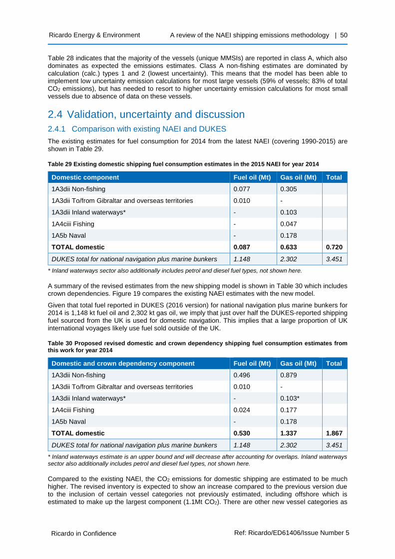
A review of the NAEI shipping emissions methodology | 50
Ricardo in Confidence Ref: Ricardo/ED61406/Issue Number 5
Ricardo Energy & Environment
Table 28 indicates that the majority of the vessels (unique MMSIs) are reported in class A, which also dominates as expected the emissions estimates. Class A non-fishing estimates are dominated by calculation (calc.) types 1 and 2 (lowest uncertainty). This means that the model has been able to implement low uncertainty emission calculations for most large vessels (59% of vessels; 83% of total CO2 emissions), but has needed to resort to higher uncertainty emission calculations for most small vessels due to absence of data on these vessels.
2.4 Validation, uncertainty and discussion
2.4.1 Comparison with existing NAEI and DUKES
The existing estimates for fuel consumption for 2014 from the latest NAEI (covering 1990-2015) are shown in Table 29.
Table 29 Existing domestic shipping fuel consumption estimates in the 2015 NAEI for year 2014
Domestic component Fuel oil (Mt) Gas oil (Mt) Total
1A3dii Non-fishing 0.077 0.305
1A3dii To/from Gibraltar and overseas territories 0.010 -
1A3dii Inland waterways* - 0.103
1A4ciii Fishing - 0.047
1A5b Naval - 0.178
TOTAL domestic 0.087 0.633 0.720
DUKES total for national navigation plus marine bunkers 1.148 2.302 3.451
* Inland waterways sector also additionally includes petrol and diesel fuel types, not shown here.
A summary of the revised estimates from the new shipping model is shown in Table 30 which includes crown dependencies. Figure 19 compares the existing NAEI estimates with the new model.
Given that total fuel reported in DUKES (2016 version) for national navigation plus marine bunkers for 2014 is 1,148 kt fuel oil and 2,302 kt gas oil, we imply that just over half the DUKES-reported shipping fuel sourced from the UK is used for domestic navigation. This implies that a large proportion of UK international voyages likely use fuel sold outside of the UK.
Table 30 Proposed revised domestic and crown dependency shipping fuel consumption estimates from this work for year 2014
Domestic and crown dependency component Fuel oil (Mt) Gas oil (Mt) Total
1A3dii Non-fishing 0.496 0.879
1A3dii To/from Gibraltar and overseas territories 0.010 -
1A3dii Inland waterways* - 0.103*
1A4ciii Fishing 0.024 0.177
1A5b Naval - 0.178
TOTAL domestic 0.530 1.337 1.867
DUKES total for national navigation plus marine bunkers 1.148 2.302 3.451
* Inland waterways estimate is an upper bound and will decrease after accounting for overlaps. Inland waterways sector also additionally includes petrol and diesel fuel types, not shown here.
Compared to the existing NAEI, the CO2 emissions for domestic shipping are estimated to be much higher. The revised inventory is expected to show an increase compared to the previous version due to the inclusion of certain vessel categories not previously estimated, including offshore which is estimated to make up the largest component (1.1Mt CO2). There are other new vessel categories as
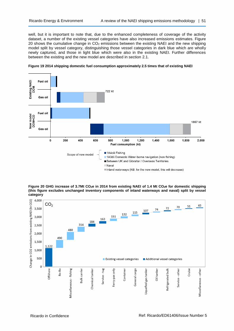
A review of the NAEI shipping emissions methodology | 51
Ricardo in Confidence Ref: Ricardo/ED61406/Issue Number 5
Ricardo Energy & Environment
well, but it is important to note that, due to the enhanced completeness of coverage of the activity dataset, a number of the existing vessel categories have also increased emissions estimates. Figure 20 shows the cumulative change in CO2 emissions between the existing NAEI and the new shipping model split by vessel category, distinguishing those vessel categories in dark blue which are wholly newly captured, and those in light blue which were also in the existing NAEI. Further differences between the existing and the new model are described in section 2.1.
Figure 19 2014 shipping domestic fuel consumption approximately 2.5 times that of existing NAEI
Figure 20 GHG increase of 3.7Mt CO2e in 2014 from existing NAEI of 1.4 Mt CO2e for domestic shipping (this figure excludes unchanged inventory components of inland waterways and naval) split by vessel category

A review of the NAEI shipping emissions methodology | 52
Ricardo in Confidence Ref: Ricardo/ED61406/Issue Number 5
Ricardo Energy & Environment
Fishing
The existing NAEI estimates for fishing vessels in 2014 assume zero fuel oil consumption, and 47kt gas oil consumption. The revised estimates, which includes crown dependencies, are 177kt gas oil (MDO) and 24kt fuel oil (HFO), totalling 201kt fuel. This total is approximately four times the existing estimate. This relative increase is shown in Figure 21 for the fuel consumption, as well as the pollutants calculated in this study. Figure 22 compares the absolute values for fuel and pollutant emissions in the existing NAEI and the estimates in this model. Figure 21 implies the overall change in method with its fuel type assumptions and emission factor updates will lead to:
• increases in CO2 and CH4 emissions approximately commensurate with the increase in fuel consumption
• increases in NOX, N2O, PM10 and NMVOCs by a factor more than the increase in fuel consumption, i.e. an emission factor increase for these pollutants
• a large increase in SO2 emissions by much more than the commensurate increase in fuel consumption. The new model assumes 1.0% sulphur fuel is used, whereas the existing model assumed 0.1% sulphur fuel is used. One eighth of the fuel consumption is now assumed to be HFO.
Further discussion on fishing vessel emissions is included in section 2.4.5.
Other than-fishing
The existing NAEI estimates of 1A3dii domestic navigation emissions for 2014 assume 77kt fuel oil consumption, and 305kt gas oil consumption. The revised estimates, including crown dependencies are 496kt fuel oil, and 879kt gas oil, i.e. a total of 1.4Mt fuel consumption leading to 4.4 Mt CO2 emissions. The relative increases of this model compared to the existing NAEI are shown in Figure 23, and the absolute quantities in Figure 24.
The revised inventory is expected to show an increase compared to the previous work due to the inclusion of certain vessel categories not previously estimated, including offshore which is estimated to make up the largest component (1.1Mt CO2).

A review of the NAEI shipping emissions methodology | 53
Ricardo in Confidence Ref: Ricardo/ED61406/Issue Number 5
Ricardo Energy & Environment
Figure 21 Fuel and emissions estimates for fishing vessels in this study (domestic and crown dependencies) expressed as a percentage of the existing 2015 NAEI for year 2014 (domestic).
Figure 22 Comparison of estimated fishing vessel fuel consumption, CO2, SO2, NOX, CH4, N2O, PM10, and NMVOC emissions between the existing 2015 NAEI for year 2014 (domestic) and new estimates in this study (domestic and crown dependencies)

A review of the NAEI shipping emissions methodology | 54
Ricardo in Confidence Ref: Ricardo/ED61406/Issue Number 5
Ricardo Energy & Environment
Figure 23 Fuel and emissions estimates for vessels other than fishing vessels in this study (domestic and crown dependencies) expressed as a percentage of the existing 2015 NAEI for year 2014 (domestic).
Figure 24 Comparison of estimates for vessels other than fishing vessels of fuel consumption, CO2, SO2, NOX, CH4, N2O, PM10, and NMVOC emissions between the existing 2015 NAEI for year 2014 (domestic) and new estimates in this study (domestic and crown dependencies)

A review of the NAEI shipping emissions methodology | 55
Ricardo in Confidence Ref: Ricardo/ED61406/Issue Number 5
Ricardo Energy & Environment
2.4.2 Model validation with existing literature
The estimates of CO2, SO2 and NOX emissions from the new NAEI shipping model for the North Sea and English Channel only have been compared in Table 31 to estimates in literature for the same geographical scope.
One of the lead authors of IMO (2015), J.P. Jalkanen, has developed a comprehensive AIS based model of shipping emissions in European waters (Jalkanen et al (2009); Jalkanen et al (2012); Jalkanen et al (2014); and Jalkanen et al (2016)). Jalkanen’s model, called the STEAM model is the most recent AIS model identified and compared in the table. The STEAM model estimates total CO2 emissions per sea area in 2011 of: 20.7Mt in the North Sea, 6.7Mt in the English Channel, and 5.0Mt in the Irish and British Seas, among other European sea areas (Jalkanen et al., 2016). This is a subtotal of 27.4Mt for the North Sea and English Channel, and 32.4Mt CO2 for the sea areas primarily covered by this study.
The comparable figures in this study (i.e. including all domestic, crown dependency, international and transit traffic) for year 2014 are shown in Table 31. These excludes estimates for vessels which have gaps in AIS coverage at sea of more than 24 hours. The value for the North Sea and English Channel is slightly lower than Jalkanen et al (2016) at 23Mt CO2, albeit relatively similar. The NOX and SO2 estimates in this model are also lower than in Jalkanen et al (2016). The SO2 results would be expected to be lower, given that the assumptions made for sulphur content in this study derive from data supplied by UKPIA on sulphur contents of fuel sold in the UK which are lower than legislative limits, rather than the approach in Jalkanen et al that sulphur contents are exactly the legislative limits.
The remaining coverage in this work outside of the SECA covers not only the “Irish and British Seas” mentioned in Jalkanen et al (2013) but also to some degree vessels in the Bay of Biscay, Norwegian Sea and in the North East Atlantic.
Table 31 Total emissions (all traffic, not just UK domestic) in North Sea and English Channel. This model estimates (excluding position messages with gaps greater than 24 hours to subsequent messages) compared to other shipping literature
Source Model type Year of inventory CO2 NOx SO2
This work AIS 2014 23Mt 0.48 Mt 0.07 Mt
Jalkanen et al. (2016) (STEAM model)
AIS 2011 27Mt 0.65 Mt 0.15 Mt
Norwegian Met. Inst. (2015) (EMEP)
Combination 2013 NE 0.64 Mt ~0.13Mt
Campling P. et al (2013) Transport demand
2005 NE 0.52 Mt 0.31 Mt
Hammingh, P., Holland M. et al, (2012)
AIS 2009 21Mt 0.47 Mt 0.18 Mt
NE Not estimated
In addition to the above, Johansson et al (2013) estimate almost 4% of the fuel consumed in the North Sea is used by service ships that operate between oil rigs and ports. In this study, the equivalent figure for the vessel category Offshore is 7.6% of the total fuel consumption in the North Sea and English Channel.
2.4.3 Vessels out of range of the terrestrial AIS receiver network for long periods
The selected methodology for estimating emissions from vessels aims to estimate the emissions between consecutive AIS messages by assuming that the vessel continues with the same reported parameters that affect the emission estimate (speed, draught etc.) for the entire period until the next AIS message for that MMSI number is received. For the well-tracked (i.e. high count rate of AIS messages per time period) vessels that do not change the reported MMSI number on the AIS message, this approach works very well as a tier 3 methodology.
There are however two disadvantages with this approach. The first is when vessels go out of range of the terrestrial AIS receiver network for a long period (discussed in this section). The second is when
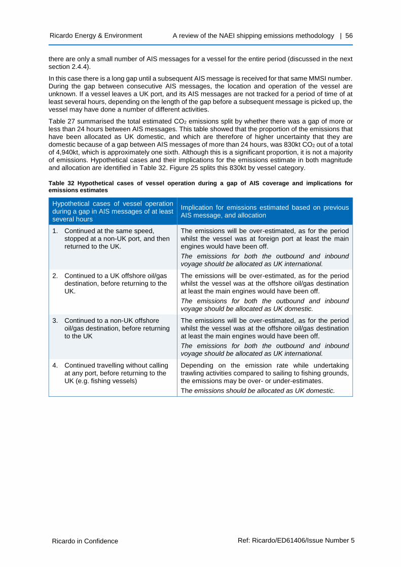
A review of the NAEI shipping emissions methodology | 56
Ricardo in Confidence Ref: Ricardo/ED61406/Issue Number 5
Ricardo Energy & Environment
there are only a small number of AIS messages for a vessel for the entire period (discussed in the next section 2.4.4).
In this case there is a long gap until a subsequent AIS message is received for that same MMSI number. During the gap between consecutive AIS messages, the location and operation of the vessel are unknown. If a vessel leaves a UK port, and its AIS messages are not tracked for a period of time of at least several hours, depending on the length of the gap before a subsequent message is picked up, the vessel may have done a number of different activities.
Table 27 summarised the total estimated CO2 emissions split by whether there was a gap of more or less than 24 hours between AIS messages. This table showed that the proportion of the emissions that have been allocated as UK domestic, and which are therefore of higher uncertainty that they are domestic because of a gap between AIS messages of more than 24 hours, was 830kt CO2 out of a total of 4,940kt, which is approximately one sixth. Although this is a significant proportion, it is not a majority of emissions. Hypothetical cases and their implications for the emissions estimate in both magnitude and allocation are identified in Table 32. Figure 25 splits this 830kt by vessel category.
Table 32 Hypothetical cases of vessel operation during a gap of AIS coverage and implications for emissions estimates
Hypothetical cases of vessel operation during a gap in AIS messages of at least several hours
Implication for emissions estimated based on previous AIS message, and allocation
1. Continued at the same speed, stopped at a non-UK port, and then returned to the UK.
The emissions will be over-estimated, as for the period whilst the vessel was at foreign port at least the main engines would have been off.
The emissions for both the outbound and inbound voyage should be allocated as UK international.
2. Continued to a UK offshore oil/gas destination, before returning to the UK.
The emissions will be over-estimated, as for the period whilst the vessel was at the offshore oil/gas destination at least the main engines would have been off.
The emissions for both the outbound and inbound voyage should be allocated as UK domestic.
3. Continued to a non-UK offshore oil/gas destination, before returning to the UK
The emissions will be over-estimated, as for the period whilst the vessel was at the offshore oil/gas destination at least the main engines would have been off.
The emissions for both the outbound and inbound voyage should be allocated as UK international.
4. Continued travelling without calling at any port, before returning to the UK (e.g. fishing vessels)
Depending on the emission rate while undertaking trawling activities compared to sailing to fishing grounds, the emissions may be over- or under-estimates.
The emissions should be allocated as UK domestic.
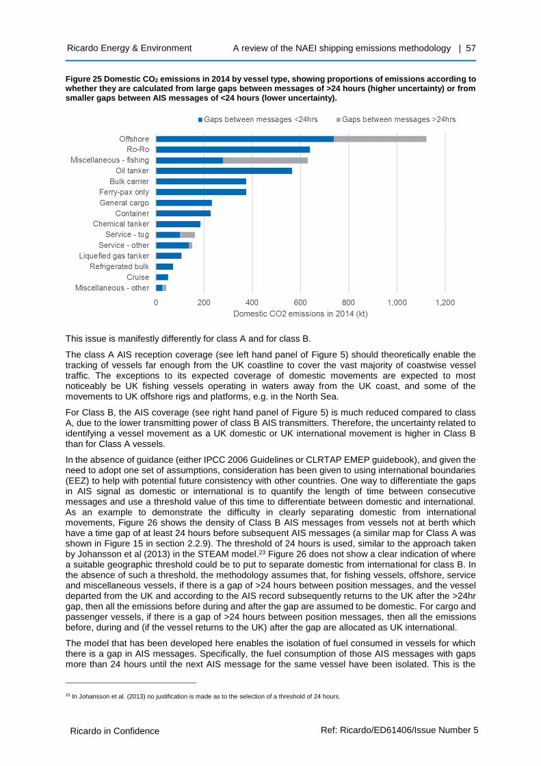
A review of the NAEI shipping emissions methodology | 57
Ricardo in Confidence Ref: Ricardo/ED61406/Issue Number 5
Ricardo Energy & Environment
Figure 25 Domestic CO2 emissions in 2014 by vessel type, showing proportions of emissions according to whether they are calculated from large gaps between messages of >24 hours (higher uncertainty) or from smaller gaps between AIS messages of <24 hours (lower uncertainty).
This issue is manifestly differently for class A and for class B.
The class A AIS reception coverage (see left hand panel of Figure 5) should theoretically enable the tracking of vessels far enough from the UK coastline to cover the vast majority of coastwise vessel traffic. The exceptions to its expected coverage of domestic movements are expected to most noticeably be UK fishing vessels operating in waters away from the UK coast, and some of the movements to UK offshore rigs and platforms, e.g. in the North Sea.
For Class B, the AIS coverage (see right hand panel of Figure 5) is much reduced compared to class A, due to the lower transmitting power of class B AIS transmitters. Therefore, the uncertainty related to identifying a vessel movement as a UK domestic or UK international movement is higher in Class B than for Class A vessels.
In the absence of guidance (either IPCC 2006 Guidelines or CLRTAP EMEP guidebook), and given the need to adopt one set of assumptions, consideration has been given to using international boundaries (EEZ) to help with potential future consistency with other countries. One way to differentiate the gaps in AIS signal as domestic or international is to quantify the length of time between consecutive messages and use a threshold value of this time to differentiate between domestic and international. As an example to demonstrate the difficulty in clearly separating domestic from international movements, Figure 26 shows the density of Class B AIS messages from vessels not at berth which have a time gap of at least 24 hours before subsequent AIS messages (a similar map for Class A was shown in Figure 15 in section 2.2.9). The threshold of 24 hours is used, similar to the approach taken by Johansson et al (2013) in the STEAM model.23 Figure 26 does not show a clear indication of where a suitable geographic threshold could be to put to separate domestic from international for class B. In the absence of such a threshold, the methodology assumes that, for fishing vessels, offshore, service and miscellaneous vessels, if there is a gap of >24 hours between position messages, and the vessel departed from the UK and according to the AIS record subsequently returns to the UK after the >24hr gap, then all the emissions before during and after the gap are assumed to be domestic. For cargo and passenger vessels, if there is a gap of >24 hours between position messages, then all the emissions before, during and (if the vessel returns to the UK) after the gap are allocated as UK international.
The model that has been developed here enables the isolation of fuel consumed in vessels for which there is a gap in AIS messages. Specifically, the fuel consumption of those AIS messages with gaps more than 24 hours until the next AIS message for the same vessel have been isolated. This is the
23 In Johansson et al. (2013) no justification is made as to the selection of a threshold of 24 hours.
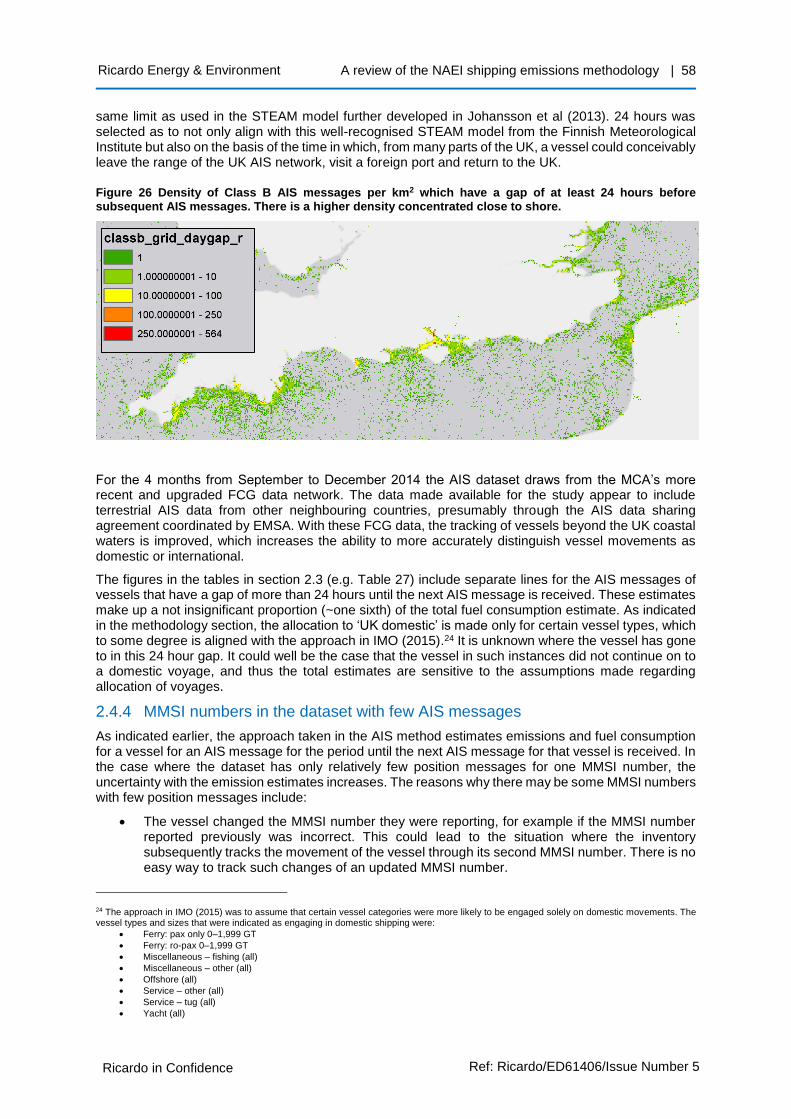
A review of the NAEI shipping emissions methodology | 58
Ricardo in Confidence Ref: Ricardo/ED61406/Issue Number 5
Ricardo Energy & Environment
same limit as used in the STEAM model further developed in Johansson et al (2013). 24 hours was selected as to not only align with this well-recognised STEAM model from the Finnish Meteorological Institute but also on the basis of the time in which, from many parts of the UK, a vessel could conceivably leave the range of the UK AIS network, visit a foreign port and return to the UK.
Figure 26 Density of Class B AIS messages per km2 which have a gap of at least 24 hours before subsequent AIS messages. There is a higher density concentrated close to shore.
For the 4 months from September to December 2014 the AIS dataset draws from the MCA’s more recent and upgraded FCG data network. The data made available for the study appear to include terrestrial AIS data from other neighbouring countries, presumably through the AIS data sharing agreement coordinated by EMSA. With these FCG data, the tracking of vessels beyond the UK coastal waters is improved, which increases the ability to more accurately distinguish vessel movements as domestic or international.
The figures in the tables in section 2.3 (e.g. Table 27) include separate lines for the AIS messages of vessels that have a gap of more than 24 hours until the next AIS message is received. These estimates make up a not insignificant proportion (~one sixth) of the total fuel consumption estimate. As indicated in the methodology section, the allocation to ‘UK domestic’ is made only for certain vessel types, which to some degree is aligned with the approach in IMO (2015).24 It is unknown where the vessel has gone to in this 24 hour gap. It could well be the case that the vessel in such instances did not continue on to a domestic voyage, and thus the total estimates are sensitive to the assumptions made regarding allocation of voyages.
2.4.4 MMSI numbers in the dataset with few AIS messages
As indicated earlier, the approach taken in the AIS method estimates emissions and fuel consumption for a vessel for an AIS message for the period until the next AIS message for that vessel is received. In the case where the dataset has only relatively few position messages for one MMSI number, the uncertainty with the emission estimates increases. The reasons why there may be some MMSI numbers with few position messages include:
• The vessel changed the MMSI number they were reporting, for example if the MMSI number reported previously was incorrect. This could lead to the situation where the inventory subsequently tracks the movement of the vessel through its second MMSI number. There is no easy way to track such changes of an updated MMSI number.
24 The approach in IMO (2015) was to assume that certain vessel categories were more likely to be engaged solely on domestic movements. The vessel types and sizes that were indicated as engaging in domestic shipping were:
• Ferry: pax only 0–1,999 GT
• Ferry: ro-pax 0–1,999 GT
• Miscellaneous – fishing (all)
• Miscellaneous – other (all)
• Offshore (all)
• Service – other (all)
• Service – tug (all)
• Yacht (all)

A review of the NAEI shipping emissions methodology | 59
Ricardo in Confidence Ref: Ricardo/ED61406/Issue Number 5
Ricardo Energy & Environment
• The vessel travelled only briefly within range of terrestrial AIS. Presumably this would not be counted as domestic in any case.
• The vessel switched on or off their AIS transceiver.
• The vessel was not operating (e.g. dry docked) for a larger period of the year with no operating AIS.
Given that the methodology estimates emissions for each position message based on the time until the subsequent position message (vessels at berth capped at maximum of 24 hours), however long that period is, there is a risk of estimating high emissions for those MMSIs with few position messages, in the cases where those position messages lead to long time gaps.
For Class A which make up the majority of total emissions, 4.8% of the domestic and crown dependency CO2 emissions are from MMSI numbers for which there are only 20 or fewer position messages – shown in Figure 27. Given the position messages are sampled at 1 per 5 minutes, 20 position messages is equivalent annual coverage of the vessel’s movements of 0.02%.25 Note that the emissions distribution in these figures has not been updated to remove the excluded calculation type 6 vessels, which would be expected to reduce the number of erroneous MMSIs.
Figure 27 Class A histogram of distribution of number of position messages per MMSI, and with the distribution of these MMSI’s contribution to domestic and crown dependency CO2 emissions.
2.4.5 Fishing vessels
Emissions from fishing vessels that land fish in the UK are categorised under IPCC guidance as source category 1A4ciii. This is all counted as UK domestic not UK international. Previous inventory review comments suggested that fishing vessel emission estimates from the Entec (2010) study were lower than perhaps expected.
Estimates for fishing vessels departing and returning to the UK include the entire period whilst the vessel is out of AIS signal as domestic.
The existing NAEI fishing emission estimates comprise two elements. The first was for activity of fishing vessels in UK waters, as covered by Entec (2010). The estimate in Entec (2010) was a top-down estimate for all small vessels and fishing vessels between 100GT and 500GT and was simply estimated as 5% of the total fuel consumption of the other vessel categories. The second was for activity of UK fishing vessels that travel to waters outside of the scope covered in Entec (2010) – e.g. off the coast of Greenland, or Morocco, which was made using a series of assumptions for the number of fishing vessels, the fuel consumption rate of the vessels, where the vessels were travelling, and how long and
25 Due to the additional thinning of stationary messages that is undertaken in Stage 3 of the model, this % coverage estimate is actually an underestimate as we have 100% confidence in a vessel’s location whilst it’s at berth.
0.0%
20.0%
40.0%
60.0%
80.0%
100.0%
0
1,000
2,000
3,000
4,000
5,000
1-10 11-20 21-50 51-100 101-1000 >1000
% o
f C
lass
A C
O2
est
imat
e
Nu
mb
er o
f M
MSI
s in
eac
h b
in
Bins: Number of position messages per MMSI
Number of MMSIs
% CO2 totaldomestic and CD

A review of the NAEI shipping emissions methodology | 60
Ricardo in Confidence Ref: Ricardo/ED61406/Issue Number 5
Ricardo Energy & Environment
how fast they would travel. The second estimate covering fishing in non-UK waters is the dominant estimate, comprising around 90% of the total fishing emissions estimate. The existing NAEI estimates are shown in Table 33.
Table 33 Existing 2014 NAEI fuel consumption estimates for fishing for year 2014
Domestic component Gas oil (kt) Fuel oil (kt)
Fishing – In UK waters 4 0
Fishing – Outside UK waters 43 0
Total fishing 47 0
As the approach taken in the AIS method estimates emissions and fuel consumption for a vessel from an AIS message for the period until the next AIS message for that vessel is received, the new model AIS approach is suitable not only for tracking UK fishing vessels in range but also for replacing the separate estimate in the NAEI for fishing outside UK waters, as long as the emissions are allocated to the UK as domestic. For fishing vessels these remain allocated to the UK if the previous country of call was the UK and the next country of call was the UK, regardless of the time gap between position messages.
Table 34 New AIS model estimates for fishing for year 2014 as total of domestic and crown dependency
Component Gas oil (kt) Fuel oil (kt) Total fuel (kt)
AIS message gaps <24 hours – assumed comparable to ‘in UK waters’
82 6 88
At sea, AIS message gap >24 hrs – assumed comparable to ‘outside UK waters’
94 18 112
Total fishing 177 24 201
The new results in Table 34 (total fuel consumption, 201kt) are in total higher than the previous estimates in Table 33 (47kt) – markedly for the component which is in range (with message gaps less than 24 hours) of the UK terrestrial AIS network compared to the existing total for ‘in UK waters’.
In this work, the number of vessels in the entire dataset (including those which did not call at the UK), which were reported either by Clarksons or in the AIS voyage messages themselves as fishing vessels, totalled 3,197 vessels (shown below in Table 35). Given that this number includes non-UK fishing vessels that happen to be in range of the terrestrial AIS (i.e. not UK domestic), this number of vessels appears to be lower than other estimates, particularly for the smaller vessels:
• UK sea fisheries statistics for 2014 (MMO, 2015) indicates the UK fleet to have 6,383 fishing vessels, made up of 5,026 10 metre and under vessels and 1,357 over 10 metre vessels.
• Coello et al (2015) use an estimate of 6,434 fishing vessels licenced under the UK flag from May 2012 to May 2013, from EU sources.
• AEA (2011) assumed 4,823 commercial fishing vessels and a further ~1,800 dive/fishing charter workboats
Table 35 summarises some statistics on the fishing fleet derived from the inventory. Coupled with the above comparisons, and noting that in section 1.4.1 it is identified that only fishing vessels above 15m are obliged to use AIS, suggests that the number of fishing vessels identified in this study is likely to include a large proportion of non-UK fishing vessels, and that there is incomplete coverage of the UK’s <10m fishing fleet.
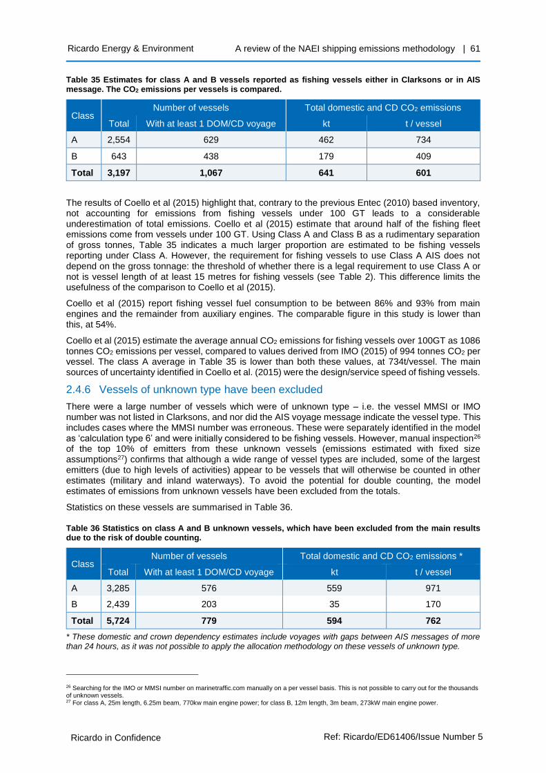
A review of the NAEI shipping emissions methodology | 61
Ricardo in Confidence Ref: Ricardo/ED61406/Issue Number 5
Ricardo Energy & Environment
Table 35 Estimates for class A and B vessels reported as fishing vessels either in Clarksons or in AIS message. The CO2 emissions per vessels is compared.
Class Number of vessels Total domestic and CD CO2 emissions
Total With at least 1 DOM/CD voyage kt t / vessel
A 2,554 629 462 734
B 643 438 179 409
Total 3,197 1,067 641 601
The results of Coello et al (2015) highlight that, contrary to the previous Entec (2010) based inventory, not accounting for emissions from fishing vessels under 100 GT leads to a considerable underestimation of total emissions. Coello et al (2015) estimate that around half of the fishing fleet emissions come from vessels under 100 GT. Using Class A and Class B as a rudimentary separation of gross tonnes, Table 35 indicates a much larger proportion are estimated to be fishing vessels reporting under Class A. However, the requirement for fishing vessels to use Class A AIS does not depend on the gross tonnage: the threshold of whether there is a legal requirement to use Class A or not is vessel length of at least 15 metres for fishing vessels (see Table 2). This difference limits the usefulness of the comparison to Coello et al (2015).
Coello et al (2015) report fishing vessel fuel consumption to be between 86% and 93% from main engines and the remainder from auxiliary engines. The comparable figure in this study is lower than this, at 54%.
Coello et al (2015) estimate the average annual CO2 emissions for fishing vessels over 100GT as 1086 tonnes CO2 emissions per vessel, compared to values derived from IMO (2015) of 994 tonnes CO2 per vessel. The class A average in Table 35 is lower than both these values, at 734t/vessel. The main sources of uncertainty identified in Coello et al. (2015) were the design/service speed of fishing vessels.
2.4.6 Vessels of unknown type have been excluded
There were a large number of vessels which were of unknown type – i.e. the vessel MMSI or IMO number was not listed in Clarksons, and nor did the AIS voyage message indicate the vessel type. This includes cases where the MMSI number was erroneous. These were separately identified in the model as ‘calculation type 6’ and were initially considered to be fishing vessels. However, manual inspection26 of the top 10% of emitters from these unknown vessels (emissions estimated with fixed size assumptions27) confirms that although a wide range of vessel types are included, some of the largest emitters (due to high levels of activities) appear to be vessels that will otherwise be counted in other estimates (military and inland waterways). To avoid the potential for double counting, the model estimates of emissions from unknown vessels have been excluded from the totals.
Statistics on these vessels are summarised in Table 36.
Table 36 Statistics on class A and B unknown vessels, which have been excluded from the main results due to the risk of double counting.
Class Number of vessels Total domestic and CD CO2 emissions *
Total With at least 1 DOM/CD voyage kt t / vessel
A 3,285 576 559 971
B 2,439 203 35 170
Total 5,724 779 594 762
* These domestic and crown dependency estimates include voyages with gaps between AIS messages of more than 24 hours, as it was not possible to apply the allocation methodology on these vessels of unknown type.
26 Searching for the IMO or MMSI number on marinetraffic.com manually on a per vessel basis. This is not possible to carry out for the thousands of unknown vessels. 27 For class A, 25m length, 6.25m beam, 770kw main engine power; for class B, 12m length, 3m beam, 273kW main engine power.
A review of the NAEI shipping emissions methodology | 62
Ricardo in Confidence Ref: Ricardo/ED61406/Issue Number 5
Ricardo Energy & Environment
2.4.7 Vessels of category Yachts have been excluded
The AIS-based model has been run to include estimates for vessels allocated to the ‘yacht’ category. For class A, vessels in this category include large ‘super yachts’, whilst the class B vessels include more common recreational vessels of sailing boats and motor cruisers. Theoretically this could include any of the EMEP guidebook suggested subcategories of recreational vessels, either with in-board engines or outboard engines. This includes sailing boats with auxiliary engines, yawls or cabin boats, speed boats, and motor boats. It may include vessels on inland waterways, depending on the range of the AIS receivers.
After allocation of the vessels with reported vessel type (either in Clarksons or in the AIS message) into vessel categories, the AIS dataset includes AIS messages from 2,540 unique Class A vessels and 7,026 unique Class B vessels in vessel category ‘yachts’. There is also a number of vessels of unknown vessel category (5,724), which could include yachts given the large number of vessels in the yachts category (see discussion in section 2.4.6).
However, comparisons of this number of recreational vessels with other sources suggests there is incomplete capture by AIS of all recreational craft activity – i.e. not all recreational craft which have engines are using AIS.
Previous work for the NAEI (AEA, 2011) assumed for the UK there are:
• ~20,600 sailing boats with auxiliary engines
• ~80,000 motorboats on inland waterways
• ~85,000 coastal motorboats, made up of:
o ~26,300 coastal power boats
o ~24,800 coastal day motorboats
o ~16,400 coastal other motorboats
o ~13,000 coastal RIBS/Inflatables or sports boats
o ~3,800 coastal hire boats
o ~900 coastal trip/restaurant boats
o ~100 coastal passenger boats
A more recent UK publication by RYA (2014) estimates that there are around 541,000 ‘leisure boats’ in the UK, which includes small sail boats, sailing yachts, power boats and motor yachts.
ICOMIA (2016) produce a recreational boating industry statistical publication. Although this publication has not been purchased, its sample pages for Germany provide an insight into the orders of magnitude for a nearby country. ICOMIA (2016) estimate that in Germany there are around 195,000 sail boats, 193,000 inboard motor boats and around 117,000 other rigid boats including outboard motorboats – totalling around 505,000.
The above review suggests that AIS may not be an appropriate tool to measure activity of vessels in the ‘yacht’ category. It may be that relatively few yachts (sail or powered) are fitted with AIS transponders, and the above numbers support this. So if the AIS method was used to estimate fuel consumption and emissions from yachts, it would likely be an estimate of a small part of the total and would need to be extrapolated up to represent all activity.
Therefore it is concluded that the existing estimates for the ‘yacht’ category as estimated in AEA (2011) should prevail, and the AIS model estimate is not used. Specifically, the totals from that methodology for the following subcategories should instead be used as ‘yachts’:
• 01. Sailing boats with auxiliary engines
• 02. Motorboats – inland waterways
• 02. Motorboats – coastal excluding Coastal Passenger vessels >12 passengers
Nevertheless, the AIS-based model has been retained to model the AIS messages from ‘yachts’ in order to gain an understanding of the geographical distribution of the AIS yacht activity data, which can be used to geographically distribute the emissions otherwise estimated from the method in AEA (2011).

A review of the NAEI shipping emissions methodology | 63
Ricardo in Confidence Ref: Ricardo/ED61406/Issue Number 5
Ricardo Energy & Environment
2.4.8 Availability of vessel characteristics data limiting calculations (Calculation types)
The methodology described in 2.2.7 describes how the emission calculations vary according to the level of data available for the vessel in question. In particular, 7 levels of calculation methods were described. The calculation types with most certainty are those where the fewest assumptions were necessary relating to the vessel in question – calculation types 1 and 2. The calculation types with the most uncertainty are types 3, 4, 5, 6 and 7. The split of the total CO2 emissions allocated to domestic and crown dependencies by calculation type is shown in Figure 28 (calculation type 7 does not appear as only exists for international movements). The figure shows that around 83% of the total CO2 estimate from both class A and B is estimated from the most certain calculation types of 1 or 2. This is an important conclusion from this new approach because even the 83% of the total estimates of emissions which have the greatest level of confidence considerably exceed the current estimates of domestic shipping emissions in the NAEI.
Figure 28 Total CO2 emissions for all vessel categories excluding yachts split by calculation (‘calc’) type.
There is higher uncertainty in the AIS reported vessel draught than in the AIS reported speed, as described in section 1.4. The implication of this is that the instantaneous main engine power demand as estimated in step 1 in section 2.2.8 will have increased uncertainty associated with it.
2.4.9 Locations of ports and other destinations
The correct identification of the location of ports and other destinations – such as offshore locations – is needed to identify when vessels are to be considered ‘at berth’ for the purposes of sulphur emissions, as well as to identify the start and end points of vessel movements which underpins the classification as domestic.
For this study, a comprehensive list of UK ports was provided by the DfT. This included coordinates of each port. However, ports and the locations in those ports where vessels might be ‘at berth’, vary in size and shape, which means that representing a port as a single set of coordinates or with a fixed distance buffer around the coordinates can be limiting. To mitigate against this, we have as part of this study replaced the single coordinate pair approach with bespoke GIS polygon mapping of around 35 of the UK’s largest ports.
The locations of the offshore platforms (principally but not exclusively in the North Sea) were identified from a dataset provided by BEIS (Pers. Comm.). To avoid capturing traffic passing offshore platforms as stopping at the platforms, a smaller distance buffer around the platforms than used for land ports has been used. In addition, a dataset on the locations in 2014 of Floating Production Storage and Offloading (FPSO) vessels was obtained from the MCA. These two datasets in combination were used to define possible offshore locations where stationary vessels could be considered to arrive at destinations, i.e. for those locations within the UK EEZ, voyages to and from these locations could then be included in UK domestic. However, the locations of the FPSOs included (per vessel) multiple locations during 2014 as these FPSOs were moved. However, we have had to use all the locations of the FPSOs during the whole of 2014 as possible destinations.
The limited information on international ports (fewer of them than for UK) has been mitigated through the application of the assumption that if a vessel travels within 5km of a foreign coastline, the vessel is assumed to call at that country.

A review of the NAEI shipping emissions methodology | 64
Ricardo in Confidence Ref: Ricardo/ED61406/Issue Number 5
Ricardo Energy & Environment
3 Backcasting and forecasting
This chapter describes the methodology and results for estimating historical and future shipping emissions based on the base year 2014 bottom-up inventory described in chapter 2. In this work, the backcasts are made for each year from 1990 to 2013, but the methodology is intended to serve the process of compiling the annual inventory for a new inventory year without having to repeat the lengthy process of compiling an inventory using AIS data each year. The forecasts are made for specific years 2020, 2025 and 2035.
3.1 Methodology – backcasting to 1990 and forecasting to current NAEI year
The approach to estimate historical inventories remains the same as in the existing NAEI –DfT port statistics are used as proxies for activity levels – but is refined to match the increased number of vessel categories than used previously, for example, the offshore sector.
The existing methodology in the NAEI scales the 2007 base year ship emissions inventory according to indices that are set equal to 1 for the base year. The indices account for changes in activity levels (which are relevant DfT port statistical time series) and for changes in fuel type and emission factors (including for changes related to SECAs).
Similarly in the new model, for backcasting the 2014 base year annually to 1990 and forwards to the latest current NAEI year, the overall approach accounts for variation in the following two parameters over time:
• Activity levels – using statistics as proxies to backcast fuel consumption (described in section 3.1.1)
• Emission factors (EF) and fuel type (described in section 3.1.2)
In summary the fuel consumption depends on the vessel type, year and fuel type:
𝐵𝑎𝑐𝑘𝑐𝑎𝑠𝑡 𝐹𝐶𝑣,𝑦,𝑓 = 𝐵𝑎𝑠𝑒 2014 𝐹𝐶𝑣,𝑓 × 𝐴𝑐𝑡𝑖𝑣𝑖𝑡𝑦 𝑖𝑛𝑑𝑒𝑥𝑣,𝑦
Emissions depend on the vessel type, pollutant, year, and are calculated from the fuel consumption:
𝐵𝑎𝑐𝑘𝑐𝑎𝑠𝑡 𝑒𝑚𝑖𝑠𝑠𝑖𝑜𝑛𝑣,𝑝,𝑦,𝑓 = 𝐵𝑎𝑐𝑘𝑐𝑎𝑠𝑡 𝐹𝐶𝑣,𝑦,𝑓 × 𝐵𝑎𝑠𝑒 2014 𝐸𝐹𝑣,𝑝,𝑓 × 𝐸𝐹 𝑖𝑛𝑑𝑒𝑥𝑝,𝑓,𝑦
Where
v vessel type
p pollutant
y year
f fuel type
The focus of the methodology developed in this work for 2014 emissions and the backcasting has been only UK domestic shipping emissions since these are included in the UK’s national totals as reported under UNFCCC, UNECE/CLRTAP and the NECD protocols. Emissions from UK international shipping are not included in national totals, but reported as a Memo Item. A different procedure is used to estimate these emissions based directly on international bunker fuels data reported in DUKES for all years back to 1990. Further details are given in Section 4. Emissions from transit traffic are not reported, although have been included in maps for 2014 emissions so they can be included in air quality models.

A review of the NAEI shipping emissions methodology | 65
Ricardo in Confidence Ref: Ricardo/ED61406/Issue Number 5
Ricardo Energy & Environment
3.1.1 Activity indices
The changes that have been made from the previous shipping emission back-casting approach are to:
• introduce new specific activity indices for the additional vessel categories now covered in the base year, not covered in the current inventory approach, thereby giving better representation of trends in activities for the different types of vessels, and
• update the activity indices for existing vessel categories to be more specific to the vessel type in question from the year 2000 (e.g. for container vessels instead of using statistics on “All ports freight units”, switched to using “Container traffic”)
Overall, there are now 15 vessel categories compared to the previous 8 categories that are each mapped to a DfT port statistic. This includes separating more cargo or commodity types, as previously activity data for all cargo were split only into time-series trends for unitised and non-unitised types. The statistical time series cover all years back from 2014 to 1990 and forward to the most recent year of statistics (currently 2015). In many cases, multiple statistical series need to be used if no complete series is available to cover the entire period to 1990. The specific statistical series used for each new vessel category is indicated in Table 37, against the existing index previously used. The main DfT statistics used are (DfT, 2017):
• PORT0102 UK major and minor port freight traffic, international and domestic by direction, annually: 1965 - 2014
• PORT0107 Domestic UK major port freight traffic by cargo type and direction, annually: 2000 – 2014
• PORT0202 UK major and minor ports main freight units, by route, annually: 1970 - 2014
Table 37 Summary of new activity indices
Vessel category
Activity index used in new model Separate domestic index?
[Existing vessel category] and Activity index used in existing NAEI
Bulk carrier 2000-2014: Table PORT0107 – ‘All dry bulk traffic’ [Note 1]
✓
[Bulk carrier]
Table PORT0102 [All ports freight traffic (t)] ‘All domestic’
Chemical tanker
2000-2014: Table PORT0107 – ‘Other liquid bulk products’ [Note 1]
✓ N/A
Container 2000-2014: Table PORT0107 – ‘Container traffic’ [Note 1]
✓
[Container]
Table PORT0202 [All ports freight units] ‘All coastwise’
General cargo
2000-2014: Table PORT0107 – ‘All other general cargo traffic’ [Note 1]
✓
[General cargo]
Table PORT0102 [All ports freight traffic (t)] ‘All domestic’
Liquefied gas tanker
2000-2014: Table PORT0107 – ‘liquefied gas’ [Note 1]
✓ N/A
Oil tanker 2000-2014: Table PORT0107 – ‘total of Crude Oil and Oil Products’ [Note 1]
✓
[Tanker]
Table PORT0102 [All ports freight traffic (t)] ‘All domestic’
Ferry- pax only
No change from existing approach ✓
[Passenger]
2003-2014: Table SPAS0201 - All domestic sea passengers
1994-2002: previous DfT publications of domestic sea passenger movements in Entec (2010)
1990-1993: linear trend based on 1994 to 2000.
Cruise No change from existing approach ✓ N/A

A review of the NAEI shipping emissions methodology | 66
Ricardo in Confidence Ref: Ricardo/ED61406/Issue Number 5
Ricardo Energy & Environment
Vessel category
Activity index used in new model Separate domestic index?
[Existing vessel category] and Activity index used in existing NAEI
Refrigerated bulk
2000-2014: Table PORT0107 – ‘Other dry bulk’ [Note 1]
✓ N/A
Ro-Ro 2000-2014: Table PORT0107 – ‘Roll-on/roll-off traffic’ [Note 1]
✓
[Ro-ro cargo]
Table PORT0202 [All ports freight units] ‘All coastwise’
Service - tug
2000-2014: Table PORT0107 – ‘total domestic traffic’ [Note 1]
✓ N/A
Miscellaneous - fishing
No change from existing approach No
[Fishing]
UK Sea Fisheries Statistics: Landings into the UK by UK and foreign vessels.
Offshore
Gross UK Oil and NGL Production in kt (DUKES table 3.1.1 Crude oil and petroleum products: production, imports and exports; Indigenous production of crude oil)
No N/A
Service – other
2000-2014: Table PORT0107 – ‘total domestic traffic’ [Note 1]
✓ N/A
Miscellaneous - other
2000-2014: Table PORT0107 – ‘total domestic traffic’ [Note 1]
✓
[Others]
Table PORT0102 [All ports freight traffic (t)] ‘Total all’ [domestic and international]
Note 1 – pre-2000 trend uses existing approach.
3.1.2 Changes in emission factors
3.1.2.1 Fuel type and CO2
In contrast with the existing NAEI shipping inventory, which assumes a series discontinuity between 2006 and 2007 assuming there is a substantive fuel switch from HFO to MDO at this time for compliance with the North Sea and English Channel SECA sulphur limit (reduction from prevailing global limit to 1.5%), the new model does not include this assumption. The new model rather assumes that this switch from HFO to MDO occurs as a result of the tightening in 2015 of the SECA fuel sulphur limit from 0.5% to 0.1%. This updated assumption is made on the basis of evidence that low sulphur heavy fuel oil was available to comply with the SECA fuel sulphur limits of 1.5% to 2010 and 1% from 2010 (IMO, 2010).
The requirement that fuel consumption at berth from 2010 complies with a sulphur limit of 0.1% implies the need for MDO. Therefore, in the backcasted inventory prior to 2010, any vessels that would have used HFO, save for the at berth requirement of 0.1% S fuel, are assumed prior to 2010 to use HFO.
No change is made to the CO2 factors per fuel in the backcasted inventory from the values used for 2014. This assumes there have been no changes in the carbon content of marine fuels from 1990 to 2014.
3.1.2.2 SO2 and PM
Assumptions on historical fuel sulphur contents are used to estimate the changes in SO2 and PM emission factors over time. The NAEI uses UK specific S-content data for marine fuel oil provided annually by UKPIA wherever possible. For more recent years, this provides separate factors for different grades of HFO meeting different sulphur content limits for marine fuels. Such data have not been available for MDO in recent years. For MDO used outside SECAs, the sulphur content is retained at the 1% mark for all years, typical of fuels sold back in the 1990s. Where additional legislative limits described in section 1.2.4 for certain geographical areas (SECA, at berth) apply, these are used, in particular the requirement for 0.1% S fuel in SECAs from 2015 and at berth for all sea areas from 2010. Entec (2010) also is used in the NAEI for additional sulphur contents, and between all sources for intervening years, linear interpolation is used. The assumptions are summarised by year in Table 38.
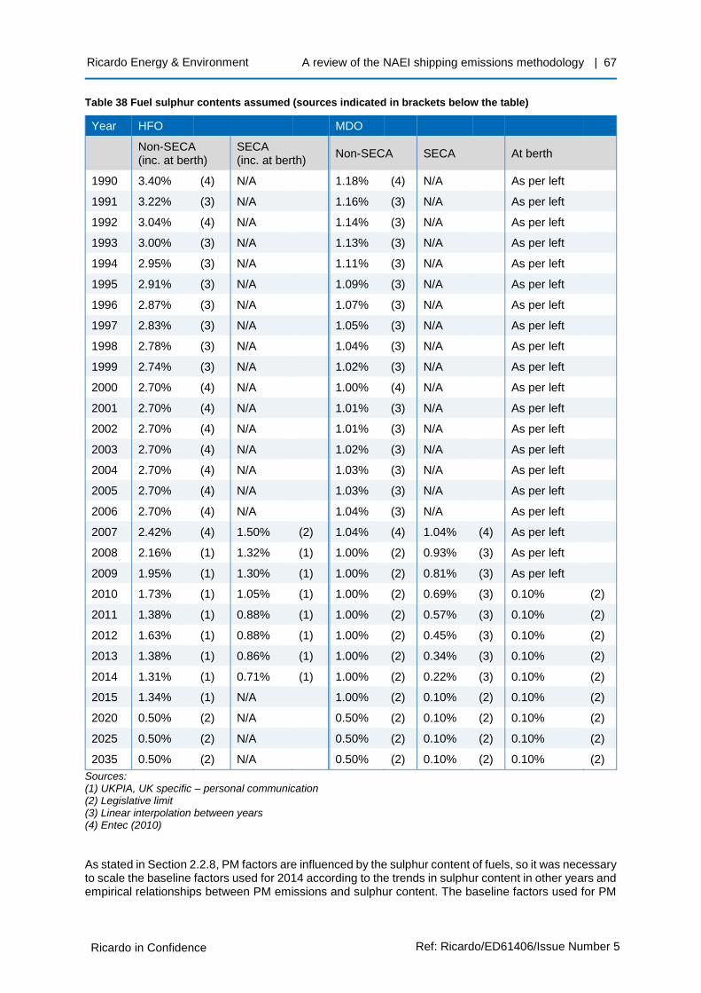
A review of the NAEI shipping emissions methodology | 67
Ricardo in Confidence Ref: Ricardo/ED61406/Issue Number 5
Ricardo Energy & Environment
Table 38 Fuel sulphur contents assumed (sources indicated in brackets below the table)
Year HFO MDO
Non-SECA (inc. at berth)
SECA (inc. at berth)
Non-SECA SECA At berth
1990 3.40% (4) N/A 1.18% (4) N/A As per left
1991 3.22% (3) N/A 1.16% (3) N/A As per left
1992 3.04% (4) N/A 1.14% (3) N/A As per left
1993 3.00% (3) N/A 1.13% (3) N/A As per left
1994 2.95% (3) N/A 1.11% (3) N/A As per left
1995 2.91% (3) N/A 1.09% (3) N/A As per left
1996 2.87% (3) N/A 1.07% (3) N/A As per left
1997 2.83% (3) N/A 1.05% (3) N/A As per left
1998 2.78% (3) N/A 1.04% (3) N/A As per left
1999 2.74% (3) N/A 1.02% (3) N/A As per left
2000 2.70% (4) N/A 1.00% (4) N/A As per left
2001 2.70% (4) N/A 1.01% (3) N/A As per left
2002 2.70% (4) N/A 1.01% (3) N/A As per left
2003 2.70% (4) N/A 1.02% (3) N/A As per left
2004 2.70% (4) N/A 1.03% (3) N/A As per left
2005 2.70% (4) N/A 1.03% (3) N/A As per left
2006 2.70% (4) N/A 1.04% (3) N/A As per left
2007 2.42% (4) 1.50% (2) 1.04% (4) 1.04% (4) As per left
2008 2.16% (1) 1.32% (1) 1.00% (2) 0.93% (3) As per left
2009 1.95% (1) 1.30% (1) 1.00% (2) 0.81% (3) As per left
2010 1.73% (1) 1.05% (1) 1.00% (2) 0.69% (3) 0.10% (2)
2011 1.38% (1) 0.88% (1) 1.00% (2) 0.57% (3) 0.10% (2)
2012 1.63% (1) 0.88% (1) 1.00% (2) 0.45% (3) 0.10% (2)
2013 1.38% (1) 0.86% (1) 1.00% (2) 0.34% (3) 0.10% (2)
2014 1.31% (1) 0.71% (1) 1.00% (2) 0.22% (3) 0.10% (2)
2015 1.34% (1) N/A 1.00% (2) 0.10% (2) 0.10% (2)
2020 0.50% (2) N/A 0.50% (2) 0.10% (2) 0.10% (2)
2025 0.50% (2) N/A 0.50% (2) 0.10% (2) 0.10% (2)
2035 0.50% (2) N/A 0.50% (2) 0.10% (2) 0.10% (2)
Sources: (1) UKPIA, UK specific – personal communication (2) Legislative limit (3) Linear interpolation between years (4) Entec (2010)
As stated in Section 2.2.8, PM factors are influenced by the sulphur content of fuels, so it was necessary to scale the baseline factors used for 2014 according to the trends in sulphur content in other years and empirical relationships between PM emissions and sulphur content. The baseline factors used for PM
A review of the NAEI shipping emissions methodology | 68
Ricardo in Confidence Ref: Ricardo/ED61406/Issue Number 5
Ricardo Energy & Environment
in 2014 correspond to sulphur contents of 2.4% for HFO and 0.14% S for MDO. These are not representative of sulphur contents of fuels used in 2014 in all sea areas and for all vessel activities around the UK coast in that year, as well as other years. The scaling of the PM factors for other sulphur content fuels shown in Table 38 was based on relationships developed by Kalli et al (2013) and shown in Entec (2010).
3.1.2.3 NOX
From the year 2000, vessel fleet average NOX emission factors are assumed to reduce by 0.7% per year due to the fleet turnover as the newer engines in the fleet that meet the IMO’s NOX technical code (MARPOL Annex VI, applied to new engines from year 2000) permeate the fleet. The value of 0.7% per year is consistent with the estimate in IVL (2016) which estimates 0.7% to 0.8% per year.
Between 1990 and 1999 the NOX emission factor is assumed to remain constant.
Both these assumptions are consistent with the existing NAEI shipping emission estimates based on Entec (2010).
In addition, any fuel switches between HFO and MDO account for the 6% difference in NOX emission factor (described in section 2.2.8.6).
3.1.2.4 VOC, CO, CH4, N2O
Emission factors for these pollutants are assumed to be static with time.
3.2 Methodology – forecasting to 2020, 2025 and 2035
For forecasting the 2014 base year as projections, the overall approach accounts for variation in the following three parameters over time:
• Activity levels
• Efficiency of maritime transport
• Emission factors (EF)
No account is taken of possible structural changes in the industry or geographic/distributional changes related to route changes (e.g. increased use of the northern sea routes).
In summary the future forecast for fuel consumption depends on the vessel type, year and fuel type:
𝐹𝑜𝑟𝑒𝑐𝑎𝑠𝑡 𝐹𝐶𝑣,𝑦,𝑓 = 𝐵𝑎𝑠𝑒 2014 𝐹𝐶𝑣,𝑓 × 𝐸𝑓𝑓𝑖𝑐𝑖𝑒𝑛𝑐𝑦 𝑖𝑛𝑑𝑒𝑥𝑦 × 𝐴𝑐𝑡𝑖𝑣𝑖𝑡𝑦 𝑖𝑛𝑑𝑒𝑥𝑣,𝑦
Forecasts of emissions depend on the vessel type, pollutant, year:
𝐹𝑜𝑟𝑒𝑐𝑎𝑠𝑡 𝑒𝑚𝑖𝑠𝑠𝑖𝑜𝑛𝑣,𝑝,𝑦 = 𝐹𝑜𝑟𝑒𝑐𝑎𝑠𝑡 𝐹𝐶𝑣,𝑦,𝑓 × 𝐵𝑎𝑠𝑒 2014 𝐸𝐹𝑣,𝑝,𝑓 × 𝐸𝐹 𝑖𝑛𝑑𝑒𝑥𝑝,𝑓,𝑦
Where
v vessel type
p pollutant
y year
f fuel type
This method is in line with Kalli et al (2013). In addition to the above methods, selected port specific projections are also made using local rather than national assumptions of Activity indices. This is described further below.
3.2.1 Activity indices
Previous maritime transport projections used in the IMO’s 1st and 2nd global GHG studies have been based on forecasts of GDP. The current NAEI projections have assumed a 1% per annum growth in fuel consumption from the latest base year (currently 2015), the same growth rate assumed by Entec (2010). The BEIS energy projections (EEP2016) appear to forecast approximately static CO2 emissions from domestic shipping. The latest Economic and fiscal outlook by the Office for Budget Responsibility (OBR, 2017) shows GDP year on year increase was 2.2% in 2015, 1.8% in 2016, and forecast to be

A review of the NAEI shipping emissions methodology | 69
Ricardo in Confidence Ref: Ricardo/ED61406/Issue Number 5
Ricardo Energy & Environment
2.0% in 2017, dropping to 1.6% and 1.7% in 2018 and 2019 respectively, before increasing again to 1.9% in 2020 and 2.0% in 2021.
IMO (2015) identifies that basing future shipping activity projections on forecast GDP change is a basic method, and that a more advanced method separates different cargo types. However, few recent literature studies that are publicly available were identified that stipulate forecasts of specific cargo types which are relevant or specific to the UK.
Three sources of information have been identified to support the selection of annual activity change factors. These are: DfT statistics of recent trends; qualitative descriptions from the company that developed the previous Government forecasts of port demand; and information from selected individual ports. The three sources are described below and their information summarised in Table 39 for cargo and passenger vessels. It is noted that the three sources do not agree with one another for many of the vessel categories.
DfT statistics
In addition to drawing on literature, the most recent DfT maritime statistics28 on port freight can be used to show the latest trends for total freight and domestic freight using statistical tables PORT0104 and PORT0107 respectively. Passenger movements domestically can be checked with table SPAS0201 and cruise passengers SPAS0101. Care must be taken however in using short term changes which may be influenced by short term fluctuations as trend analysis, but they can form part of the judgement on future trends.
Qualitative descriptions
The most recent Government forecasts of demand for port capacity appear to still be those by MDS Transmodal published in 2007.29 In the absence of updated forecasts, additional commentary since then by MDS Transmodal (2011), which accounts for the impacts of the economic recession, suggests:
• UK maritime sector growth rates expected to be lower than international trade average
• UK growth for international unitised tonnages: 2.5% per annum deep-sea, 1.5% for short-sea
• Coastwise (mode switch) traffic may be source of growth
• Bulk liquids and gas imports likely to be flat and coal to decline from closures of UK coal power stations
• Other general cargo - linked to forest products and steel
• Growth in ro-ro trades from the continent recovering more slowly than deep-sea trade
Further more recent UK-relevant literature identified includes IVL (2016) which suggests annual average growth rates of 1.5% for all vessel types except for container vessels. Container vessel activity annual growth rates in IVL (2016) are suggested to be 3.5%, based on work by Hammingh et al. (2012) and Kalli et al (2013). DfT’s Maritime Growth Study report (DfT, 2015) does not include suitable assumptions for forecasting the inventory.
Port level projections
Defra requested emission projections of air pollutants from shipping at seven specific ports in the UK for this project, reflecting their interest in the impact of shipping emissions on local air quality in these port areas. We were requested by Defra to investigate the plans for seven ports of Southampton, Grimsby, Immingham, Liverpool, Bristol, Felixstowe and Hull, and we contacted operators for these ports. For four ports (Southampton, Immingham, Liverpool and Felixstowe) projections of activity changes per cargo type and passenger volumes were taken from port development Master Plans published by the various port operators. For example, the Port of Southampton operated by ABP has a master plan, as a consultation document, showing projections in freight tonnage, units moved and passenger numbers for different vessel types out to 2035. No information was found to support port specific projections for the remaining three ports of Grimsby, Bristol and Hull.
The four ports’ projections generally have different trends forecast up to 2020 and slowing down thereafter. The specific port projections generally seem to have higher annual growth rates than the
28 https://www.gov.uk/government/collections/maritime-and-shipping-statistics 29 As identified in the National Policy Statement for Ports in January 2012 https://www.gov.uk/government/uploads/system/uploads/attachment_data/file/3931/national-policy-statement-ports.pdf
A review of the NAEI shipping emissions methodology | 70
Ricardo in Confidence Ref: Ricardo/ED61406/Issue Number 5
Ricardo Energy & Environment
recent historical statistics suggest. It is unclear if this difference is because of a trend towards usage of larger ports or not.
Overall assumed activity growth rates
Alongside the recent DfT statistics in annual average growth rates of activities for different vessel categories, Table 39 shows national growth rates from MDS Transmodal (2011) and the growth at each of the 7 ports based on port Master Plans. The table also shows, in the final column, the UK average annual rates of activity change derived from consideration of these three information sources, excluding shipping activity within 5km of the ports of Southampton, Immingham, Liverpool and Felixstowe. For these four specific ports, the port-specific growth rates are used to project changes in activity levels.
The existing assumptions in the NAEI for forecasting the inland waterways sector are used for the remaining non-cargo, non-passenger vessel categories of:
• Service – tug
• Miscellaneous – fishing
• Offshore
• Service – other
• Miscellaneous – other

A review of the NAEI shipping emissions methodology | 71
Ricardo in Confidence Ref: Ricardo/ED61406/Issue Number 5
Ricardo Energy & Environment
Table 39 Summary of sources DfT, MDS Transmodal and port-specific forecasts of annual average activity change by vessel type. The final column are the UK average annual rates of activity change 2014-2035
Vessel category (IMO)
Matched DfT type
Annual total change in DfT statistics
MDS Transmodal
(2011)
Felixstowe forecast annual
growth 30
Immingham forecast
annual growth
31
Liverpool forecast annual
growth 32
Southampton forecast annual
growth 33
UK average annual rate of activity
change 2014-2035
(%)
Statistics scope
2014-15
2013-15
2012-15
1 Bulk carrier All dry bulk Total 1 -15% -7.4% -2.1%
Decline - 5.8% to 2020,
0.6% after
1.5% to 2020, 1.1%
after
6% to 2020, 2.5% after
0 Domestic2 5.0% 11% 6.1%
3 Chemical tanker
Oil product Total 1 4.7% -2.4% -0.4%
Flat - 2.6% to 2020,
0.6% after No growth
(flat) 1.2% to 2020,
0.5% after 0
Domestic2 1.6% -4.1% 1.6%
4 Container Container Total 1 3.2% 5.4% 4.7%
Growth 7% to 2020, 2.9% after
8.9% to 2020, 5.5% after
9.5% to 2020, 4.1%
after 3% +4%
Domestic2 5.8% 10% 6.7%
5 General cargo
All other general cargo
Total 1 -4.1% -2.5% 3.5% Flat -
1.6% to 2020, 1.4% after
3.5% to 2020, 2.8%
after
11% to 2020, 3% after
0 Domestic2 -14% -7.4% -8.3%
6 Liquefied gas tanker
Liquefied gas
Total 1 19% 11% -1.4% Flat -
2.6% to 2020, 0.6% after
1.5% to 2020, 1.4%
after
1.2% to 2020, 0.5% after
+2% Domestic2 25% 35% 15%
7 Oil tanker Crude oil Total 1 1.4% -1.3% -4.8%
Flat - +1% Domestic2 31% 11% -5.8%
9 Ferry-pax only All domestic sea passengers
Domestic3 -2.2% -1.8% -0.3% - - - - 3% 2015 to
2035 -1%
10 Cruise All cruise passengers
Domestic4 6.7% 0.3% 3.2% - - - - 7.7% to 2020,
2% after +1%
30 Port of Felixstowe document “Future Development To ensure we continue to meet your needs. Best. Downloaded from https://www.portoffelixstowe.co.uk/#/investing-in-the-future/ 31 Port of Immingham Master Plan 2010-2030 32 Mersey Ports Master Plan 2011 consultation https://www.peelports.com/media/1534/executive-summary.pdf and https://www.peelports.com/about/master-plan 33 2016-2035 Master Plan consultation document http://www.southamptonvts.co.uk/admin/content/files/New%20capital%20projects/Master%20Plan%202016/Master%20Plan%202016%20-%202035%20Consultation%20Document%20Oct%202016.pdf. Figures for liquid bulks (#3,6,7) from previous 2009 Master Plan.

A review of the NAEI shipping emissions methodology | 72
Ricardo in Confidence Ref: Ricardo/ED61406/Issue Number 5
Ricardo Energy & Environment
Vessel category (IMO)
Matched DfT type
Annual total change in DfT statistics
MDS Transmodal
(2011)
Felixstowe forecast annual
growth 30
Immingham forecast
annual growth
31
Liverpool forecast annual
growth 32
Southampton forecast annual
growth 33
UK average annual rate of activity
change 2014-2035
(%)
Statistics scope
2014-15
2013-15
2012-15
12 Refrigerated bulk
Other dry bulk
Total 1 13% 16% 12% - - - - - +2%
Domestic2 14% 17% 10%
13 Ro-Ro Ro-Ro Total1 4.2% 4.5% 3.2%
Growth - 3.9% to 2020,
2.5% after 3.3%
5.4% to 2020, 3% after
+3% Domestic2 4.4% 3.2% 0.5%
1 Total annual tonnage change in DfT statistics table PORT0104
2 Domestic annual tonnage change in DfT statistics table PORT0107
3 Domestic annual change in number of passengers in DfT statistics table SPAS0201
4 Cruise annual change in number of passengers in DfT statistics table SPAS0101
The UK average annual rates of activity change can be represented in the following equations:
i.e. 𝐴𝑐𝑡𝑖𝑣𝑖𝑡𝑦 𝑖𝑛𝑑𝑒𝑥𝑦,𝑐𝑜𝑛𝑡𝑎𝑖𝑛𝑒𝑟 = 1.04(𝑦−2014)
i.e. 𝐴𝑐𝑡𝑖𝑣𝑖𝑡𝑦 𝑖𝑛𝑑𝑒𝑥𝑦,𝑙𝑖𝑞𝑢𝑒𝑓𝑖𝑒𝑑 𝑔𝑎𝑠 𝑡𝑎𝑛𝑘𝑒𝑟 = 1.02(𝑦−2014)
i.e. 𝐴𝑐𝑡𝑖𝑣𝑖𝑡𝑦 𝑖𝑛𝑑𝑒𝑥𝑦,𝑜𝑖𝑙 𝑡𝑎𝑛𝑘𝑒𝑟 = 1.01(𝑦−2014)
i.e. 𝐴𝑐𝑡𝑖𝑣𝑖𝑡𝑦 𝑖𝑛𝑑𝑒𝑥𝑦,𝑓𝑒𝑟𝑟𝑦−𝑝𝑎𝑥 𝑜𝑛𝑙𝑦 = 0.99(𝑦−2014)
i.e. 𝐴𝑐𝑡𝑖𝑣𝑖𝑡𝑦 𝑖𝑛𝑑𝑒𝑥𝑦,𝑐𝑟𝑢𝑖𝑠𝑒 = 1.01(𝑦−2014)
i.e. 𝐴𝑐𝑡𝑖𝑣𝑖𝑡𝑦 𝑖𝑛𝑑𝑒𝑥𝑦,𝑟𝑒𝑓𝑟𝑖𝑑𝑔𝑒𝑟𝑎𝑡𝑒𝑑 𝑏𝑢𝑙𝑘 = 1.02(𝑦−2014)
i.e. 𝐴𝑐𝑡𝑖𝑣𝑖𝑡𝑦 𝑖𝑛𝑑𝑒𝑥𝑦,𝑅𝑜−𝑅𝑜 = 1.03(𝑦−2014)

A review of the NAEI shipping emissions methodology | 73
Ricardo in Confidence Ref: Ricardo/ED61406/Issue Number 5
Ricardo Energy & Environment
3.2.2 Emission factor index
The changes in emission factors apply to all vessel voyages, domestic, international and transit. The future operation of the North Sea as a NOX ECA is assumed to begin from 2021, i.e. requirements for new ships will begin from then. Existing ships will continue to be allowed to operate in the North Sea.
3.2.2.1 Fuel and CO2
Any HFO consumption in a SECA is assumed to switch to MDO consumption from 2015 onwards.
From 2021, a proportion of LNG powered vessels is assumed to operate in the NECA. A simple fleet turnover model is used (described for NOX below) to estimate the proportion of the fleet made up by new vessels from 2021, of which one third is assumed to be LNG, replacing HFO.
Emission factors of CO2 per tonne fuel do not change, but switches between fuel types are taken into account for CO2 emissions.
3.2.2.2 SO2
Any HFO consumption in a SECA is assumed to switch to MDO consumption from 2015 onwards, with an SO2 emission factor reduction of 90% (from 1% S HFO to 0.1% MDO). Any HFO consumption out of SECA is assumed to switch to 0.5% HFO from 2020.
Any existing consumption in 2014 of MDO (with sulphur content of 0.1%) is assumed to remain with the same fuel type and sulphur content in future years.
The SO2 emission factor for LNG was shown in section 2.2.8.7.
3.2.2.3 NOX
Future NOX emissions factors reduce over time for two reasons: first, due to continued turnover in the fleet leading to larger proportions of vessels with more recent engines which meet later (more stringent) NOX emission tiers. Secondly, due to the anticipated NOX ECA designation of the North Sea.
For the first variable, reductions from fleet turnover are expected to continue at the same approximate rate until 2020. IMO (2015) indicates NOX EF reductions of around 0.5% per year for HFO and distillate. IVL (2016) appear to indicate slightly higher reduction rates of 0.7% to 0.8% over time. The figure of 0.7% annual reduction is selected from 2014 to 2020:
𝐸𝐹 𝑖𝑛𝑑𝑒𝑥𝑁𝑂𝑥, 2014 𝑡𝑜 2021 = 0.993(𝑦−2014)
For the second variable IVL (2016) identify the compliance routes for the NOX ECA as three options: (1) in-engine design modification to use exhaust gas recirculation (EGR); (2) end-of-pipe solution of selective catalytic reduction (SCR); or (3) switch to an LNG-powered engine. However, specifying which of these compliance options may not be necessary for the inventory, as all need to meet the Tier III standard, which is an 80% reduction from Tier I levels. The key aspect to account for is the increase in reduction rate of NOX emission factor from 2021. A simple fleet turnover model has been generated to estimate suitable empirical assumptions for annual average NOX emission factor reductions from 2021.34 This shows in Figure 29 that the simple assumption of 0.7% to 2020 and then 4% per year thereafter achieves a relatively close match (in grey in the Figure) to the fleet turnover model (in blue in the Figure). The fleet average NOX emission factor is assumed to reduce by 4% per year from 2021.
𝐸𝐹 𝑖𝑛𝑑𝑒𝑥𝑁𝑂𝑥, 2021+ = 0.993(2020−2014) × 0.96(𝑦−2021)
In addition, any NOX emissions associated with HFO consumption in SECAs is assumed from 2015 to reduce by 6% accounting for the fuel type switching. 𝐸𝐹𝑀𝐷𝑂 = 0.94 ∗ 𝐸𝐹𝐻𝐹𝑂
34 A simple fleet turnover model assuming 2014 fleet mix comprises 36% Tier 0, 43% Tier I and 21% Tier II engines based on mix of ages from known vessels in Clarksons vessel characteristics database, and assuming vessel lifetime of 25 years (i.e. 4% replacement rate each year), and assuming EFs as stipulated in section 2.2.8.6, and assuming Tier III EF is 80% lower than Tier I EF.
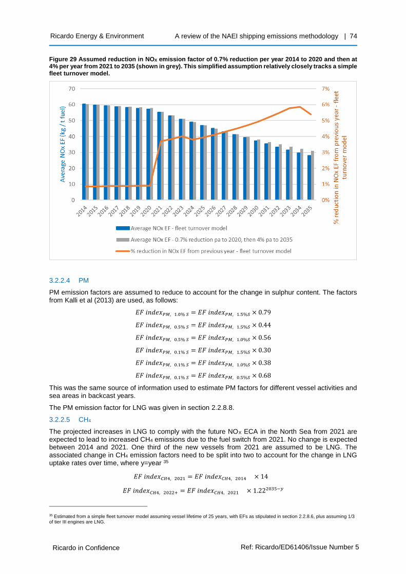
A review of the NAEI shipping emissions methodology | 74
Ricardo in Confidence Ref: Ricardo/ED61406/Issue Number 5
Ricardo Energy & Environment
Figure 29 Assumed reduction in NOX emission factor of 0.7% reduction per year 2014 to 2020 and then at 4% per year from 2021 to 2035 (shown in grey). This simplified assumption relatively closely tracks a simple fleet turnover model.
3.2.2.4 PM
PM emission factors are assumed to reduce to account for the change in sulphur content. The factors from Kalli et al (2013) are used, as follows:
𝐸𝐹 𝑖𝑛𝑑𝑒𝑥𝑃𝑀, 1.0% 𝑆 = 𝐸𝐹 𝑖𝑛𝑑𝑒𝑥𝑃𝑀, 1.5%𝑆 × 0.79
𝐸𝐹 𝑖𝑛𝑑𝑒𝑥𝑃𝑀, 0.5% 𝑆 = 𝐸𝐹 𝑖𝑛𝑑𝑒𝑥𝑃𝑀, 1.5%𝑆 × 0.44
𝐸𝐹 𝑖𝑛𝑑𝑒𝑥𝑃𝑀, 0.5% 𝑆 = 𝐸𝐹 𝑖𝑛𝑑𝑒𝑥𝑃𝑀, 1.0%𝑆 × 0.56
𝐸𝐹 𝑖𝑛𝑑𝑒𝑥𝑃𝑀, 0.1% 𝑆 = 𝐸𝐹 𝑖𝑛𝑑𝑒𝑥𝑃𝑀, 1.5%𝑆 × 0.30
𝐸𝐹 𝑖𝑛𝑑𝑒𝑥𝑃𝑀, 0.1% 𝑆 = 𝐸𝐹 𝑖𝑛𝑑𝑒𝑥𝑃𝑀, 1.0%𝑆 × 0.38
𝐸𝐹 𝑖𝑛𝑑𝑒𝑥𝑃𝑀, 0.1% 𝑆 = 𝐸𝐹 𝑖𝑛𝑑𝑒𝑥𝑃𝑀, 0.5%𝑆 × 0.68
This was the same source of information used to estimate PM factors for different vessel activities and sea areas in backcast years.
The PM emission factor for LNG was given in section 2.2.8.8.
3.2.2.5 CH4
The projected increases in LNG to comply with the future NOX ECA in the North Sea from 2021 are expected to lead to increased CH4 emissions due to the fuel switch from 2021. No change is expected between 2014 and 2021. One third of the new vessels from 2021 are assumed to be LNG. The associated change in CH4 emission factors need to be split into two to account for the change in LNG uptake rates over time, where y=year 35
𝐸𝐹 𝑖𝑛𝑑𝑒𝑥𝐶𝐻4, 2021 = 𝐸𝐹 𝑖𝑛𝑑𝑒𝑥𝐶𝐻4, 2014 × 14
𝐸𝐹 𝑖𝑛𝑑𝑒𝑥𝐶𝐻4, 2022+ = 𝐸𝐹 𝑖𝑛𝑑𝑒𝑥𝐶𝐻4, 2021 × 1.222035−𝑦
35 Estimated from a simple fleet turnover model assuming vessel lifetime of 25 years, with EFs as stipulated in section 2.2.8.6, plus assuming 1/3 of tier III engines are LNG.
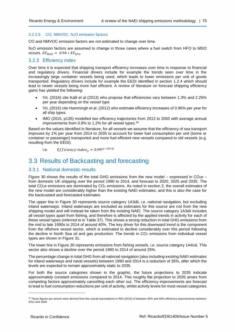
A review of the NAEI shipping emissions methodology | 75
Ricardo in Confidence Ref: Ricardo/ED61406/Issue Number 5
Ricardo Energy & Environment
3.2.2.6 CO, NMVOC, N2O emission factors
CO and NMVOC emission factors are not estimated to change over time.
N2O emission factors are assumed to change in those cases where a fuel switch from HFO to MDO occurs. 𝐸𝐹𝑀𝐷𝑂 = 0.94 ∗ 𝐸𝐹𝐻𝐹𝑂
3.2.3 Efficiency index
Over time it is expected that shipping transport efficiency increases over time in response to financial and regulatory drivers. Financial drivers include for example the trends seen over time in the increasingly large container vessels being used, which leads to lower emissions per unit of goods transported. Regulatory drivers include for example the EEDI identified in section 1.2.4 which should lead to newer vessels being more fuel efficient. A review of literature on forecast shipping efficiency gains has yielded the following:
• IVL (2016) cite Kalli et al (2013) who propose that efficiencies vary between 1.3% and 2.25% per year depending on the vessel type
• IVL (2016) cite Hammingh et al. (2012) who estimate efficiency increases of 0.96% per year for all ship types.
• IMO (2015, p135) modelled two efficiency trajectories from 2012 to 2050 with average annual improvements from 0.9% to 1.2% for all vessel types.36
Based on the values identified in literature, for all vessels we assume that the efficiency of sea transport improves by 1% per year from 2014 to 2035 to account for lower fuel consumption per unit (tonne or container or passenger) transported and more fuel efficient new vessels compared to old vessels (e.g. resulting from the EEDI).
i.e. 𝐸𝑓𝑓𝑖𝑐𝑖𝑒𝑛𝑐𝑦 𝑖𝑛𝑑𝑒𝑥𝑦 = 0.99(𝑦−2014)
3.3 Results of Backcasting and forecasting
3.3.1 National domestic results
Figure 30 shows the results of the total GHG emissions from the new model – expressed in CO2e – from domestic UK shipping over the period 1990 to 2014, and forecast to 2020, 2025 and 2035. The total CO2e emissions are dominated by CO2 emissions. As noted in section 2, the overall estimates of the new model are considerably higher than the existing NAEI estimates, and this is also the case for the backcasted and forecasted estimates.
The upper line in Figure 30 represents source category 1A3dii, i.e. national navigation, but excluding inland waterways. Inland waterways are excluded as estimates for this source are not from the new shipping model and will instead be taken from the existing NAEI. The source category 1A3dii includes all vessel types apart from fishing, and therefore is affected by the applied trends in activity for each of these vessel types (referred to in Table 37). This shows a strong reduction in total GHG emissions from the mid to late 1990s to 2014 of around 40%. The key driver for this downward trend is the component from the offshore vessel sector, which is estimated to decline considerably over this period following the decline in North Sea oil and gas production. The trends in CO2 emissions from individual vessel types are shown in Figure 31.
The lower line in Figure 30 represents emissions from fishing vessels, i.e. source category 1A4ciii. This sector also shows a decline over the period 1990 to 2014 of around 25%.
The percentage change in total GHG from all national navigation (also including existing NAEI estimates for inland waterways and naval vessels) between 1990 and 2014 is a reduction of 35%, after which the levels are expected to remain approximately static to 2035.
For both the source categories shown in the graphic, the future projections to 2035 indicate approximately constant emissions compared to 2014. This roughly flat projection to 2035 arises from competing factors approximately cancelling each other out. The efficiency improvements are forecast to lead to fuel consumption reductions per unit of activity, whilst activity levels for most vessel categories
36 These figures per annum were derived from the overall assumptions in IMO (2015) of between 40% and 60% efficiency improvements between 2012 and 2050.

A review of the NAEI shipping emissions methodology | 76
Ricardo in Confidence Ref: Ricardo/ED61406/Issue Number 5
Ricardo Energy & Environment
are expected to grow. In addition, an increase in LNG as a fuel is forecast as a means for vessel operators to comply with the more stringent NOx requirements of the NOx ECA from 2021. This increase in LNG, which is a slow increase over time as the fleet is forecast to turn over, is estimated to lead to increased CH4 emissions, also countering forecast efficiency improvements.
Figure 30 Domestic shipping GHG emissions in CO2e from 1990 to 2035, upper line for source category 1A3dii (national navigation, excluding inland waterways), lower line for 1A4ciii (fishing). Scope match to carbon budgets, i.e. crown dependencies and to/from overseas territories and Gibraltar are excluded)
Figure 31 Trend over time of offshore vessel emissions is a key driver for total 1990-2014 CO2 emissions trends for domestic shipping category 1A3dii, excluding inland waterways.

A review of the NAEI shipping emissions methodology | 77
Ricardo in Confidence Ref: Ricardo/ED61406/Issue Number 5
Ricardo Energy & Environment
The projections shown in Figure 30 of approximately no change in total GHG emissions for domestic shipping emissions have been compared to results of future scenarios of shipping emissions made by the Committee on Climate Change (CCC). The CCC’s shipping emission scenarios supporting the fifth carbon budget proposals (CCC, 2015) indicates that a tonne-miles demand forecasting approach is taken, combined with the effects of increased efficiency from the EEDI. However, the CCC (2015) does not specify the precise forecasting methodology that is used, and no distinction is described between domestic and international shipping. The CCC ‘high emissions’ scenario most closely matches the forecasts made in this study. Whilst Figure 30 shows approximately no change between 2014 and 2035 in GHG emissions from domestic shipping, the CCC (2015) forecasts a slight reduction in the total of domestic plus international shipping emissions: 2% reduction from 2015 by 2020, increasing to 5% reduction by 2025 and 8% by 2030.
Figure 32 shows in blue the estimated domestic NOX emissions backcast from 1990 to 2013, the base year model result for 2014, and the forecast emissions in 2020, 2025 and 2035. The scope of this is per the NECD reporting requirements, i.e. it includes source category 1A3dii (national navigation including inland waterways and between UK and Gibraltar), 1A4ciii (fishing) and 1A5b (naval), but excluding the Crown Dependencies and between the UK and the Overseas Territories. Also shown in Figure 32 as a green line is the existing NAEI estimates for the exact same scope as for the new model. The new model estimates 2014 NOX emissions to be 66kt higher than the existing NAEI estimates. This difference is made up of new vessel categories not previous accounted for (offshore 21kt, service-tug 4kt, chemical tanker 3kt, among others) as well as increases in existing vessel categories (fishing 11kt, RoRo 9kt, bulk carrier 7kt, among others).
There is a large estimated reduction in NOX emissions of 40% between 1990 and 2014 in the new model from 197kt to 117kt. This compares with the existing NAEI estimates of 74kt in 1990 and 51kt in 2014, which is a reduction of 31%. The steeper reduction of the new model compared to the existing estimates is driven by the new activity driver for the new category of offshore vessels.
The new model also forecasts a drop in NOx emissions from 2014, whereas the existing NAEI shows approximately static NOX emissions. The new model forecasts NOX emissions to reduce by 9% from 2014 to 2020, compared to the existing NAEI forecasting a 6% reduction between 2014 and 2020. The key change in assumptions for this difference is concerning the forecast decrease in NOX emission factors due to fleet turnover, as well as the impact of the NOX ECA from 2021 onwards.
Figure 32 Domestic shipping NOx emissions from 1990 to 2035, upper blue line for new model, low green line for existing NAEI. Includes source category 1A3dii (national navigation, including inland waterways and to/from Gibraltar), 1A4ciii (fishing) and 1A5b (naval). Scope match to NECD reporting requirements, i.e. crown dependencies and to/from overseas territories are excluded).
Similarly, to the NOX figure above, Figure 33 shows the backcast and forecast results for SO2 emissions. Apart from the generally higher emissions of the new model compared to the existing NAEI, the
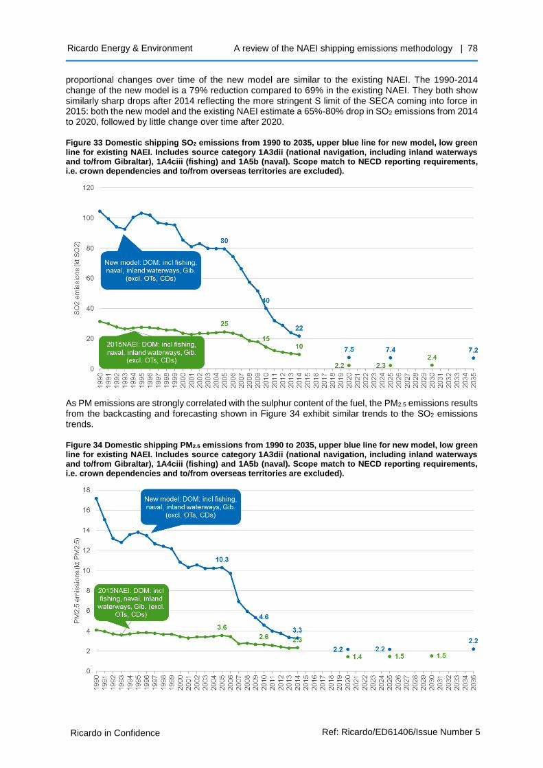
A review of the NAEI shipping emissions methodology | 78
Ricardo in Confidence Ref: Ricardo/ED61406/Issue Number 5
Ricardo Energy & Environment
proportional changes over time of the new model are similar to the existing NAEI. The 1990-2014 change of the new model is a 79% reduction compared to 69% in the existing NAEI. They both show similarly sharp drops after 2014 reflecting the more stringent S limit of the SECA coming into force in 2015: both the new model and the existing NAEI estimate a 65%-80% drop in SO2 emissions from 2014 to 2020, followed by little change over time after 2020.
Figure 33 Domestic shipping SO2 emissions from 1990 to 2035, upper blue line for new model, low green line for existing NAEI. Includes source category 1A3dii (national navigation, including inland waterways and to/from Gibraltar), 1A4ciii (fishing) and 1A5b (naval). Scope match to NECD reporting requirements, i.e. crown dependencies and to/from overseas territories are excluded).
As PM emissions are strongly correlated with the sulphur content of the fuel, the PM2.5 emissions results from the backcasting and forecasting shown in Figure 34 exhibit similar trends to the SO2 emissions trends.
Figure 34 Domestic shipping PM2.5 emissions from 1990 to 2035, upper blue line for new model, low green line for existing NAEI. Includes source category 1A3dii (national navigation, including inland waterways and to/from Gibraltar), 1A4ciii (fishing) and 1A5b (naval). Scope match to NECD reporting requirements, i.e. crown dependencies and to/from overseas territories are excluded).

A review of the NAEI shipping emissions methodology | 79
Ricardo in Confidence Ref: Ricardo/ED61406/Issue Number 5
Ricardo Energy & Environment
The picture for NMVOC emissions, shown in Figure 35 differs from the other pollutants, as VOC emissions are dominated by those from petrol combustion of inland waterways vessels, which are estimated to increase from 1990 to 2014. Nevertheless, the new domestic shipping method still leads to increased estimates of NMVOC emissions compared with current NAEI estimates.
Figure 35 Domestic shipping VOC emissions from 1990 to 2035, upper blue line for new model, low green line for existing NAEI. Includes source category 1A3dii (national navigation, including inland waterways and to/from Gibraltar), 1A4ciii (fishing) and 1A5b (naval). Scope match to NECD reporting requirements, i.e. crown dependencies and to/from overseas territories are excluded).
3.3.2 Port level trends for specific ports
The SO2, NOX, PM and VOC emission trend estimates of the port-level projections for the four ports for which specific activity drivers were identified (described in section 3.2.1) are shown in Figure 36. The aim of these port specific projections were driven by requests from Defra and encompass total traffic from all vessels (i.e. not only domestic, but also international) within a 5km radius of the ports. For comparison purposes, a plot is also included in the figure for the UK total emissions trends, although this represents only the UK domestic total.
The NOX trends show that the drivers for change in activity growth are forecast to outweigh the fleet NOX reduction factor until the NOX ECA comes into force from 2021, which then leads to overall NOX emission reductions for the three ports of the four which are within the future NECA. For SO2 emissions, all plots show reductions from 2014 to 2020, as sulphur reductions occur in 2015 for SECAs and in 2020 for outside SECAs.

A review of the NAEI shipping emissions methodology | 80
Ricardo in Confidence Ref: Ricardo/ED61406/Issue Number 5
Ricardo Energy & Environment
Figure 36 SO2, NOX, PM and VOC emission trends for each port with specific projections, covering domestic plus international traffic. Emission trend for rest of UK also shown, domestic traffic only.
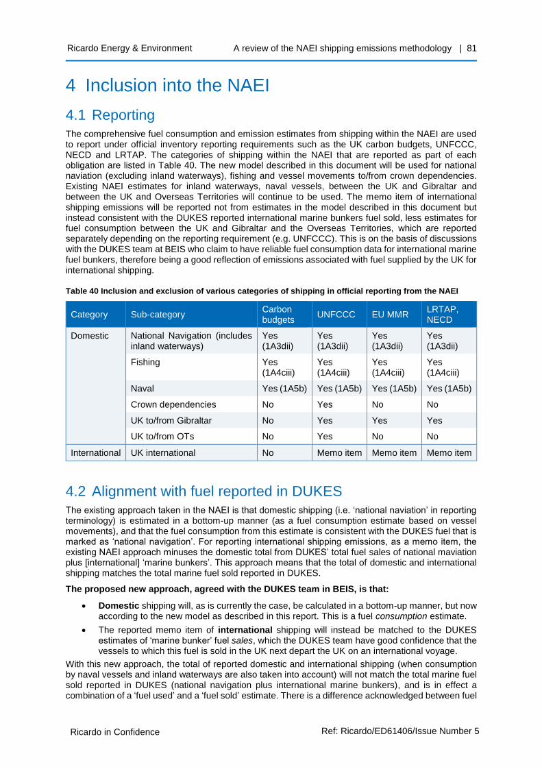
A review of the NAEI shipping emissions methodology | 81
Ricardo in Confidence Ref: Ricardo/ED61406/Issue Number 5
Ricardo Energy & Environment
4 Inclusion into the NAEI
4.1 Reporting
The comprehensive fuel consumption and emission estimates from shipping within the NAEI are used to report under official inventory reporting requirements such as the UK carbon budgets, UNFCCC, NECD and LRTAP. The categories of shipping within the NAEI that are reported as part of each obligation are listed in Table 40. The new model described in this document will be used for national naviation (excluding inland waterways), fishing and vessel movements to/from crown dependencies. Existing NAEI estimates for inland waterways, naval vessels, between the UK and Gibraltar and between the UK and Overseas Territories will continue to be used. The memo item of international shipping emissions will be reported not from estimates in the model described in this document but instead consistent with the DUKES reported international marine bunkers fuel sold, less estimates for fuel consumption between the UK and Gibraltar and the Overseas Territories, which are reported separately depending on the reporting requirement (e.g. UNFCCC). This is on the basis of discussions with the DUKES team at BEIS who claim to have reliable fuel consumption data for international marine fuel bunkers, therefore being a good reflection of emissions associated with fuel supplied by the UK for international shipping.
Table 40 Inclusion and exclusion of various categories of shipping in official reporting from the NAEI
Category Sub-category Carbon budgets
UNFCCC EU MMR LRTAP, NECD
Domestic National Navigation (includes inland waterways)
Yes (1A3dii)
Yes (1A3dii)
Yes (1A3dii)
Yes (1A3dii)
Fishing Yes (1A4ciii)
Yes (1A4ciii)
Yes (1A4ciii)
Yes (1A4ciii)
Naval Yes (1A5b) Yes (1A5b) Yes (1A5b) Yes (1A5b)
Crown dependencies No Yes No No
UK to/from Gibraltar No Yes Yes Yes
UK to/from OTs No Yes No No
International UK international No Memo item Memo item Memo item
4.2 Alignment with fuel reported in DUKES
The existing approach taken in the NAEI is that domestic shipping (i.e. ‘national naviation’ in reporting terminology) is estimated in a bottom-up manner (as a fuel consumption estimate based on vessel movements), and that the fuel consumption from this estimate is consistent with the DUKES fuel that is marked as ‘national navigation’. For reporting international shipping emissions, as a memo item, the existing NAEI approach minuses the domestic total from DUKES’ total fuel sales of national maviation plus [international] ‘marine bunkers’. This approach means that the total of domestic and international shipping matches the total marine fuel sold reported in DUKES.
The proposed new approach, agreed with the DUKES team in BEIS, is that:
• Domestic shipping will, as is currently the case, be calculated in a bottom-up manner, but now according to the new model as described in this report. This is a fuel consumption estimate.
• The reported memo item of international shipping will instead be matched to the DUKES estimates of ‘marine bunker’ fuel sales, which the DUKES team have good confidence that the vessels to which this fuel is sold in the UK next depart the UK on an international voyage.
With this new approach, the total of reported domestic and international shipping (when consumption by naval vessels and inland waterways are also taken into account) will not match the total marine fuel sold reported in DUKES (national navigation plus international marine bunkers), and is in effect a combination of a ‘fuel used’ and a ‘fuel sold’ estimate. There is a difference acknowledged between fuel

A review of the NAEI shipping emissions methodology | 82
Ricardo in Confidence Ref: Ricardo/ED61406/Issue Number 5
Ricardo Energy & Environment
used and fuel sold, in that vessel operators that subsequently engage on UK domestic voyages may well have bought the fuel to be used on that UK journey previously from elsewhere (e.g. Rotterdam) due to the fuel price differential.
The change in the approach for reporting emissions for domestic and international shipping has been taken for two main reasons. The first is that, without taking this approach, for some years in the backcast time series (1999 to 2003) the new model domestic fuel consumption estimate alone exceeds the sum total of the DUKES estimates of total marine fuel solid (sum of national navigation and international marine bunkers) – shown in Figure 37. The second reason is that, due to the way the DUKES marine fuel sales data are collected, there is higher confidence in the DUKES’ estimates of the international ‘marine bunkers’ fuel sales than the portion allocated to national navigation, such that these fuel used data are preferred by BEIS to be used for domestic shipping. Notwithstanding the uncertainty in DUKES’ own estimates of fuel sold for national navigation, the higher amount of fuel consumed from this study for domestic shipping may imply that a significant amount of fuel used for domestic voyages was sourced from overseas.
Since the purpose of the new estimates of domestic shipping fuel consumption and emissions is to provide the most accurate estimates for reporting inventories – according to definitions defined by international guidelines which must include domestic emissions but not international shipping emissions in the national totals – our approach is considered to be the best way of utilising these two different sets of information.
Figure 37 New model domestic estimate of fuel consumption exceeds DUKES total marine fuel sold (international marine bunkers plus national navigation) for years 1999, 2000, 2002 (sum of fuel oil and distillate)
A review of the NAEI shipping emissions methodology | 83
Ricardo in Confidence Ref: Ricardo/ED61406/Issue Number 5
Ricardo Energy & Environment
5 References
ABPmer (2014) White paper ‘Making Best Use of AIS Data; The value of AIS to planning and management. ABP Marine Environmental Research. Available from www.abpmer.co.uk
AEA (2010) HFC consumption and emissions forecasting containing an update to the June 2008 HFC projections.
AEA (2011) Greenhouse Gas Emissions from Inland Waterways and Recreational Craft in the UK https://uk-air.defra.gov.uk/assets/documents/reports/cat07/1106231031_IP_Task_25_Inland_Waterways_Issue_1.pdf
American Petroleum Institute (2015) Liquefied Natural Gas (LNG) Operations: Consistent Methodology for estimating greenhouse gas emissions: prepared by the LEVON Group LLC., Washington DC.
Balduzzi, M., Pasta, A., Wilhoit, K. (2014) A security evaluation of AIS automated identification system. Proceedings of the 30th Annual Computer Security Applications Conference, pp 436-445. http://citeseerx.ist.psu.edu/viewdoc/download?doi=10.1.1.694.7968&rep=rep1&type=pdf
Campling P., Janssen L., Vanherle K., Cofala J., Heyes C., and Sander R. (2013) Specific evaluation of emissions from shipping including assessment for the establishment of possible new emission control areas in European Seas. VITO Final report for European Commission. http://ec.europa.eu/environment/air/pdf/Main%20Report%20Shipping.pdf
CCC (2015) Sectoral scenarios for the Fifth Carbon Budget. Technical Report. Committee on Climate Change. https://www.theccc.org.uk/wp-content/uploads/2015/11/Sectoral-scenarios-for-the-fifth-carbon-budget-Committee-on-Climate-Change.pdf
DfT (2015) Maritime Growth Study: keeping the UK competitive in a global market. September 2015. https://www.gov.uk/government/collections/maritime-growth-study
DfT (2017) Maritime and Shipping Statistics. Downloaded from https://www.gov.uk/government/collections/maritime-and-shipping-statistics
ECG (2013) Sulphur content in marine fuels, Briefing Report, p8. http://www.ecgassociation.eu/Portals/0/Documentation/Publications/ECGBriefingReport_SulphurContent_Jan2013.pdf
EEA (2017) Air pollutant emissions data viewer (LRTAP Convention). Last modified 12 Jul 2017. http://www.eea.europa.eu/data-and-maps/data/data-viewers/air-emissions-viewer-lrtap
EMEP/EEA (2016) Air pollutant emission inventory guidebook – 2016. EEA Report No 21/2016 http://www.eea.europa.eu/publications/emep-eea-guidebook-2016
Entec (2002) Quantification of emissions from ships associated with ship movements between ports in the European Community. http://ec.europa.eu/environment/air/pdf/chapter1_ship_emissions.pdf
Entec (2010) UK ship emissions inventory. Final report. November 2010. https://uk-air.defra.gov.uk/assets/documents/reports/cat15/1012131459_21897_Final_Report_291110.pdf
Greene, W.H. (2011) Econometric Analysis, 7th ed, Pearson Education.
Hammingh, P. Holland M. et al, (2012). Assessment of the environmental impacts and health benefits of a nitrogen emission control area in the North Sea, PBL Netherlands Environmental Assessment Agency. http://www.pbl.nl/sites/default/files/cms/publicaties/pbl-2012-assessment-of-the-environmental-impacts-and-health-benefits-of-a-nitrogen-emission-control-area-in-the-north-sea-500249001-v2_0.pdf
ICOMIA (2016) Recreational Boating Industry Statistics 2015. Sample pages for Germany. Available from http://www.icomia.com/library/Default.aspx?LibraryDocumentId=1583
A review of the NAEI shipping emissions methodology | 84
Ricardo in Confidence Ref: Ricardo/ED61406/Issue Number 5
Ricardo Energy & Environment
IMO (2002). SOLAS Chapter V, Regulation 19.2 – Carriage requirements for shipborne navigational systems and equipment.
IMO (2008). MEPC 57/4/24, 8 February 2008, Sulphur monitoring for 2007.
IMO (2009). MEPC 59/4/1, 3 February 2009, Sulphur monitoring for 2008.
IMO (2010). MEPC 61/4, 16 February 2010, Sulphur monitoring for 2009.
IMO (2010b) Study To Review Assessments Undertaken Of The Revised MARPOL Annex VI Regulations. MEPC 61/INF.10
IMO (2011). MEPC 62/4, 28 February 2011, Sulphur monitoring for 2010.
IMO (2012)a. MEPC 63/23, Annex 8, 2012 Guidelines on the Method of Calculation of the Attained Energy Efficiency Design Index (EEDI) for New Ships.
IMO (2012)b. MEPC 64/4, 19 March 2012, Sulphur monitoring for 2011.
IMO (2013). MEPC 65/4/9, 26 February 2013, Sulphur monitoring programme for fuel oils for 2012.
IMO (2014)b. Special Areas under MARPOL, International Maritime Organization retrieved March 2014 from http://www.imo.org/OurWork/Environment/PollutionPrevention/SpecialAreasUnderMARPOL/Pages/Default.aspx.
IMO (2014)c. Press Briefings, IMO Marine Environment Protection Committee completes 66th session, 10, April 7, 2014, International Maritime Organization retrieved March 2014 from http://www.imo.org/MediaCentre/PressBriefings/Pages/10-MEPC-66-ends.aspx#.U3NJndJDFoA.
IMO (2014)d. Nitrogen Oxides (NOx) – Regulation 13, International Maritime Organization retrieved March 2014 from http://www.imo.org/OurWork/Environment/PollutionPrevention/AirPollution/Pages/Nitrogen-oxides-(NOx)-%E2%80%93-Regulation-13.aspx.
IMO (2015) Third IMO Greenhouse Gas 2014 study. Smith, T. W. P.; Jalkanen, J. P.; Anderson, B. A.; Corbett, J. J.; Faber, J.; Hanayama, S.; O’Keeffe, E.; Parker, S.; Johansson, L.; Aldous, L.; Raucci, C.; Traut, M.; Ettinger, S.; Nelissen, D.; Lee, D. S.; Ng, S.; Agrawal, A.; Winebrake, J. J.; Hoen, M.; Chesworth, S.; Pandey, A.
IPCC (2006) Guidelines for National Greenhouse Gas Inventories. Volume 2 Energy. http://www.ipcc-nggip.iges.or.jp/public/2006gl/
IVL (2004) Cooper, D., Gustafsson, T., Methodology for calculating emissions from ships: 1. Update of emission factors, IVL (Swedish Environmental Research Institute).
IVL (2016) NOx controls for shipping in EU Seas. Report for Transport Environment, by IVL and CE Delft. https://www.transportenvironment.org/sites/te/files/publications/2016_Consultant_report_shipping_NOx_abatement.pdf
Jalkanen, J.-P., Brink, A., Kalli, J., Pettersson, H., Kukkonen, J., and Stipa, T. (2009) A modelling system for the exhaust emissions of marine traffic and its application in the Baltic Sea area, Atmos. Chem. Phys., 9, 9209-9223, doi:10.5194/acp-9-9209-2009.
Jalkanen, J.-P., Johansson, L., Kukkonen, J., Brink, A., Kalli, J. and Stipa, T. (2012) Extension of an assessment model of ship traffic exhaust emissions for particulate matter and carbon monoxide, Journal of Atmospheric Chemistry and Physics, 12, 2641–2659.
Jalkanen, J.-P., Johansson L. and Kukkonen, J. (2014) A comprehensive inventory of the ship traffic exhaust emissions in the Baltic Sea from 2006 to 2009, Ambio, 43, 311–324.
Jalkanen, J.-P., Johansson, L., Kukkonen, J. (2016) A comprehensive inventory of ship traffic exhaust emissions in the European sea areas in 2011, Journal of Atmospheric Chemistry and Physics, 16, 71–84.

A review of the NAEI shipping emissions methodology | 85
Ricardo in Confidence Ref: Ricardo/ED61406/Issue Number 5
Ricardo Energy & Environment
Johansson, L., Jalkanen, J.-P., Kalli, J., and Kukkonen, J. (2013) The evolution of shipping emissions and the costs of regulation changes in the northern EU area. Journal of Atmospheric Chemistry and Physics, 13, 11375–11389
Kalli, J., Jalkanen, J. P., Johansson, L., & Repka, S. (2013) Atmospheric emissions of European SECA shipping: long-term projections. WMU Journal of Maritime Affairs, 2013(12), 129-145.
Kristensen H. O. (2012) Energy demand and exhaust gas emissions of marine engines, Project No. 2010–56, Emissionsbeslutningsstøttesystem, Work Package 2, Report No. 05, September.
Marine Scotland (2014) Mapping Vessel Movements from Satellite AIS. Report by ABPmer, R/4226/1. Downloaded from http://www.gov.scot/Resource/0045/00452579.pdf
MARINTEK (2010) Nielsen. J.B., Stenersen,O. Emission factors for CH4, NOx, particulates, and black carbon for domestic shipping in Norway, revision 1, Report MT22 A 10-199.
MARINTEK (2014) Einang, Per Magne, LNG som drivstoff for skip – fremtidig utveckling, Nordic Gas Conference.
MCA (2003) MSN 1768 ships' medical stores: application of the merchant shipping and fishing vessels (medical stores) regulations 1995 (SI 1995/1802) and the amendment regulations 1996 (SI 1996/2821). Maritime and Coastguard Agency. https://www.gov.uk/government/publications/msn-1768-applying-the-ships-medical-stores-regulations-1995
MDS Transmodal (2011) Future Demand and Capacity Projections. Presentation given at UK Ports Policy conference: http://www.mdst.co.uk/attachments/downloads/211001_presentation_final.pdf
MMO (2013) Spatial trends in shipping activity. Marine Management Organisation project number 1042. Available from http://webarchive.nationalarchives.gov.uk/20140108121958/http://www.marinemanagement.org.uk/evidence/documents/1042.pdf
MMO (2014) Mapping UK shipping density and routes from AIS. Marine Management Organisation project number 1066. Available from https://www.gov.uk/government/uploads/system/uploads/attachment_data/file/317770/1066.pdf
MMO (2015) UK Sea Fisheries Statistics 2014. Marine Management Organisation. Downloaded from https://www.gov.uk/government/uploads/system/uploads/attachment_data/file/462753/UK_Sea_Fisheries_Statistics_2014_-_online_version.pdf
NGA (2016) World Port Index (Pub 150) – Maritime Safety Information. http://msi.nga.mil/NGAPortal/MSI.portal?_nfpb=true&_pageLabel=msi_portal_page_62&pubCode=0015
Norwegian Met. Inst. (2015) EMEP status Report 1/2015 ‘Transboundary particulate matter, photo-oxidants, acidifying and eutrophying components’. Data from EU Horizon2020 project MACC-III http://emep.int/publ/reports/2015/EMEP_Status_Report_1_2015.pdf
OBR (2017) Economic and fiscal outlook. March 2017. Office for Budget Responsibility http://budgetresponsibility.org.uk/efo/economic-fiscal-outlook-march-2017/
Porathe, T. (2013) The North Sea today. Presentation within ACCSEAS: e-Navigation Test-Bed in the North Sea Region project. Chalmers University of Technology, Sweden. Downloaded September 2015 from http://www.accseas.eu/content/download/503/3837/file/05%2520-%2520Porathe%2520-%2520WP%25203%2520findings%2520FINAL.pdf
RYA (2014) Economic Contribution of the Recreational Boater. Royal Yachting Association. Downloaded from http://www.rya.org.uk/SiteCollectionDocuments/legal/Web%20Documents/Environment/Economic_Contribution_From_Recreational_Boating.pdf
Sarvi, A, Fogelholm, C.J. and Zevenhoven, R. (2008). Emissions from large-scale medium-speed diesel engines: 1. Influence of engine operation mode and turbocharger, Fuel Processing Technology, 89, 510–519.

A review of the NAEI shipping emissions methodology | 86
Ricardo in Confidence Ref: Ricardo/ED61406/Issue Number 5
Ricardo Energy & Environment
Starcrest (2013). Port of Los Angeles Inventory of Air Emissions 2012, Available: http://www.portoflosangeles.org/pdf/2012_Air_Emissions_Inventory.pdf
Wärtsilä (2011). Haraldson, L. LNG as a fuel for environmentally friendly shipping, 33rd Motorship Propulsion & Emissions Conference, Copenhagen, Denmark.
Wärtsilä (2014). Solutions for marine and oil and gas markets.
World Bank (2013). DataBank. Website: http://databank.worldbank.org/data/views/reports/tableview.aspx.
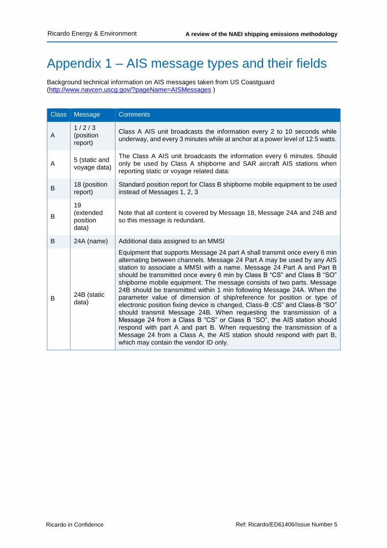
A review of the NAEI shipping emissions methodology
Ricardo in Confidence Ref: Ricardo/ED61406/Issue Number 5
Ricardo Energy & Environment
Appendix 1 – AIS message types and their fields
Background technical information on AIS messages taken from US Coastguard (http://www.navcen.uscg.gov/?pageName=AISMessages )
Class Message Comments
A 1 / 2 / 3 (position report)
Class A AIS unit broadcasts the information every 2 to 10 seconds while underway, and every 3 minutes while at anchor at a power level of 12.5 watts.
A 5 (static and voyage data)
The Class A AIS unit broadcasts the information every 6 minutes. Should only be used by Class A shipborne and SAR aircraft AIS stations when reporting static or voyage related data:
B 18 (position report)
Standard position report for Class B shipborne mobile equipment to be used instead of Messages 1, 2, 3
B
19 (extended position data)
Note that all content is covered by Message 18, Message 24A and 24B and so this message is redundant.
B 24A (name) Additional data assigned to an MMSI
Equipment that supports Message 24 part A shall transmit once every 6 min alternating between channels. Message 24 Part A may be used by any AIS station to associate a MMSI with a name. Message 24 Part A and Part B should be transmitted once every 6 min by Class B “CS” and Class B “SO” shipborne mobile equipment. The message consists of two parts. Message 24B should be transmitted within 1 min following Message 24A. When the parameter value of dimension of ship/reference for position or type of electronic position fixing device is changed, Class-B :CS” and Class-B “SO” should transmit Message 24B. When requesting the transmission of a Message 24 from a Class B “CS” or Class B “SO”, the AIS station should respond with part A and part B. When requesting the transmission of a Message 24 from a Class A, the AIS station should respond with part B, which may contain the vendor ID only.
B 24B (static data)
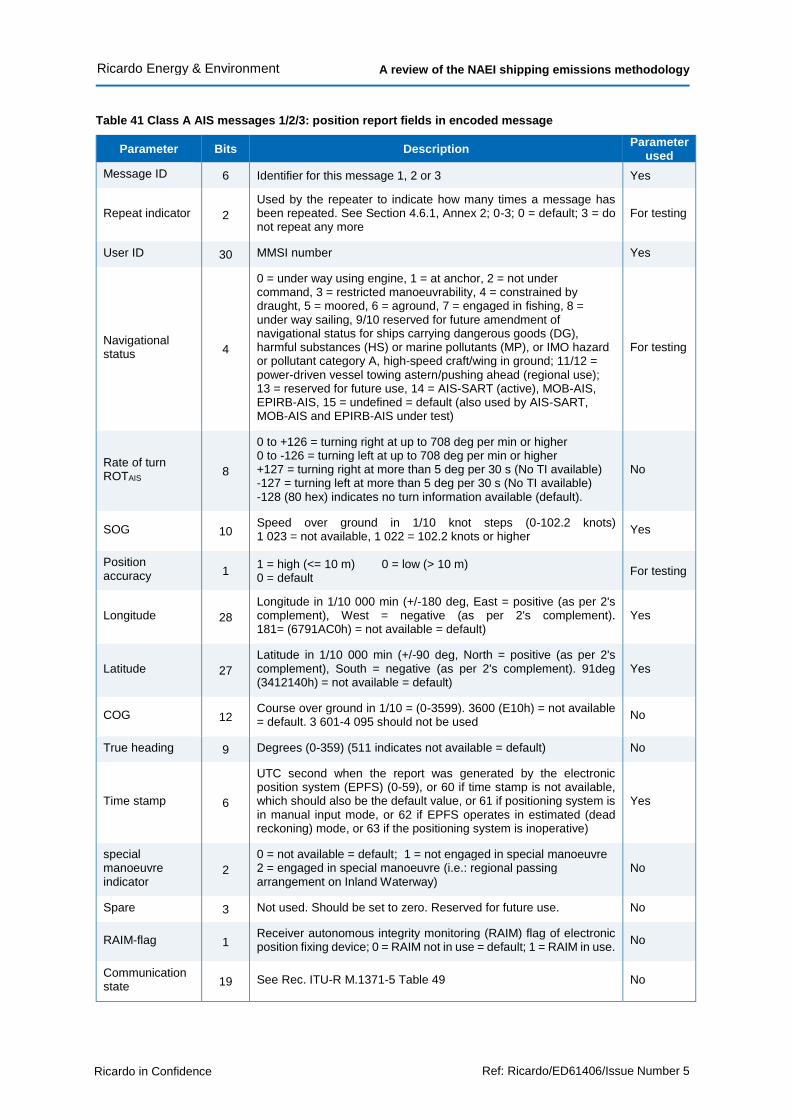
A review of the NAEI shipping emissions methodology
Ricardo in Confidence Ref: Ricardo/ED61406/Issue Number 5
Ricardo Energy & Environment
Table 41 Class A AIS messages 1/2/3: position report fields in encoded message
Parameter Bits Description Parameter
used
Message ID 6 Identifier for this message 1, 2 or 3 Yes
Repeat indicator 2
Used by the repeater to indicate how many times a message has been repeated. See Section 4.6.1, Annex 2; 0-3; 0 = default; 3 = do not repeat any more
For testing
User ID 30 MMSI number Yes
Navigational status 4
0 = under way using engine, 1 = at anchor, 2 = not under command, 3 = restricted manoeuvrability, 4 = constrained by draught, 5 = moored, 6 = aground, 7 = engaged in fishing, 8 = under way sailing, 9/10 reserved for future amendment of navigational status for ships carrying dangerous goods (DG), harmful substances (HS) or marine pollutants (MP), or IMO hazard or pollutant category A, high-speed craft/wing in ground; 11/12 = power-driven vessel towing astern/pushing ahead (regional use); 13 = reserved for future use, 14 = AIS-SART (active), MOB-AIS, EPIRB-AIS, 15 = undefined = default (also used by AIS-SART, MOB-AIS and EPIRB-AIS under test)
For testing
Rate of turn ROTAIS 8
0 to +126 = turning right at up to 708 deg per min or higher 0 to -126 = turning left at up to 708 deg per min or higher +127 = turning right at more than 5 deg per 30 s (No TI available) -127 = turning left at more than 5 deg per 30 s (No TI available) -128 (80 hex) indicates no turn information available (default).
No
SOG 10 Speed over ground in 1/10 knot steps (0-102.2 knots) 1 023 = not available, 1 022 = 102.2 knots or higher
Yes
Position accuracy 1
1 = high (<= 10 m) 0 = low (> 10 m) 0 = default
For testing
Longitude 28
Longitude in 1/10 000 min (+/-180 deg, East = positive (as per 2's complement), West = negative (as per 2's complement). 181= (6791AC0h) = not available = default)
Yes
Latitude 27
Latitude in 1/10 000 min (+/-90 deg, North = positive (as per 2's complement), South = negative (as per 2's complement). 91deg (3412140h) = not available = default)
Yes
COG 12 Course over ground in 1/10 = (0-3599). 3600 (E10h) = not available = default. 3 601-4 095 should not be used
No
True heading 9 Degrees (0-359) (511 indicates not available = default) No
Time stamp 6
UTC second when the report was generated by the electronic position system (EPFS) (0-59), or 60 if time stamp is not available, which should also be the default value, or 61 if positioning system is in manual input mode, or 62 if EPFS operates in estimated (dead reckoning) mode, or 63 if the positioning system is inoperative)
Yes
special manoeuvre indicator
2
0 = not available = default; 1 = not engaged in special manoeuvre 2 = engaged in special manoeuvre (i.e.: regional passing arrangement on Inland Waterway)
No
Spare 3 Not used. Should be set to zero. Reserved for future use. No
RAIM-flag 1 Receiver autonomous integrity monitoring (RAIM) flag of electronic position fixing device; 0 = RAIM not in use = default; 1 = RAIM in use.
No
Communication state 19 See Rec. ITU-R M.1371-5 Table 49 No

A review of the NAEI shipping emissions methodology
Ricardo in Confidence Ref: Ricardo/ED61406/Issue Number 5
Ricardo Energy & Environment
Table 42 – Class A AIS message type 5: static and voyage data
Parameter Bits Description Parameter
used Message ID 6 Identifier for this Message 5 Yes
Repeat indicator 2
Used by the repeater to indicate how many times a message has been repeated. Refer to §?4.6.1, Annex 2; 0-3; 0 = default; 3 = do not repeat any more
For testing
User ID 30 MMSI number Yes
AIS version indicator 2
0 = station compliant with Recommendation ITU-R M.1371-1 1 = station compliant with Recommendation ITU-R M.1371-3 (or later) 2 = station compliant with Recommendation ITU-R M.1371-5 (or later) 3 = station compliant with future editions
No
IMO number 30
0 = not available = default 0000000001-0000999999 not used 0001000000-0009999999 = valid IMO number; 0010000000-1073741823 = official flag state number.
Yes
Call sign 42 7 6bit ASCII characters, @@@@@@@ = not available = default.
No
Name 120
Maximum 20 characters 6 bit ASCII "@@@@@@@@@@@@@@@@@@@@" = not available = default The Name should be as shown on the station radio license.
For testing
Type of ship and cargo type 8
0 = not available or no ship = default 1-99 = as defined below 100-199 = reserved, for regional use 200-255 = reserved, for future use
Yes
Overall dimension/ reference for position
30 Reference point for reported position. Also indicates the dimension of ship (m)
Yes
Type of electronic position fixing device
4
0 = undefined (default) 1 = GPS 2 = GLONASS 3 = combined GPS/GLONASS 4 = Loran-C 5 = Chayka 6 = integrated navigation system 7 = surveyed 8 = Galileo, 9-14 = not used 15 = internal GNSS
No
ETA 20
Estimated time of arrival; MMDDHHMM UTC Bits 19-16: month; 1-12; 0 = not available = default Bits 15-11: day; 1-31; 0 = not available = default Bits 10-6: hour; 0-23; 24 = not available = default Bits 5-0: minute; 0-59; 60 = not available = default
For testing
Maximum present static draught
8 In 1/10 m, 255 = draught 25.5 m or greater, 0 = not available = default; in accordance with IMO Resolution A.851
Yes
Destination 120 Maximum 20 characters using 6-bit ASCII; @@@@@@@@@@@@@@@@@@@@ = not available
For testing
DTE 1 Data terminal equipment (DTE) ready (0 = available, 1 = not available = default)
No
Spare 1 Spare. Not used. Should be set to zero. Reserved for future use.
No
Number of bits 424 Occupies 2 slots

A review of the NAEI shipping emissions methodology
Ricardo in Confidence Ref: Ricardo/ED61406/Issue Number 5
Ricardo Energy & Environment
Table 43 – AIS message type 18: Class B position report fields
Parameter Bits Description Parameter
used Message ID 6 Identifier for Message 18; always 18 Yes
Repeat indicator 2 Used by the repeater to indicate how many times a message has been repeated; 0-3; 0 = default; 3 = do not repeat anymore; should be 0 for “CS” transmissions
Yes
User ID 30 MMSI number Yes Spare 8 Not used. Should be set to zero. Reserved for future use No
SOG 10 Speed over ground in 1/10 knot steps (0-102.2 knots) 1 023 = not available, 1 022 = 102.2 knots or higher
Yes
Position accuracy 1 1 = high (<= 10 m) 0 = low (> 10 m) 0 = default
For testing
Longitude 28 Longitude in 1/10 000 min (+180º, East = positive (as per 2's complement)), West = negative (as per 2's complement); 181º (6791AC0h) = not available = default)
Yes
Latitude 27 Latitude in 1/10 000 min (90º, North = positive (as per 2's complement)), South = negative (as per 2's complement); 91º = (3412140h) = not available = default)
Yes
COG 12 Course over ground in 1/10= (0-3 599). 3 600 (E10h) = not available = default; 3 601-4 095 should not be used
No
True heading 9 Degrees (0-359) (511 indicates not available = default) No
Time stamp 6
UTC second when the report was generated by the EPFS (0-59 or 60 if time stamp is not available, which should also be the default value or 61 if positioning system is in manual input mode or 62 if electronic position fixing system operates in estimated (dead reckoning) mode or 63 if the positioning system is inoperative) 61, 62, 63 are not used by "CS" AIS
Yes
Spare 2 Not used. Should be set to zero. Reserved for future use No
Class B unit flag 1 0 = Class B SOTDMA unit 1 = Class B "CS" unit
No
Class B display flag 1
0 = No display available; not capable of displaying Message 12 and 14 1 = Equipped with integrated display displaying Message 12 and 14
No
Class B DSC flag 1 0 = Not equipped with DSC function 1 = Equipped with DSC function (dedicated or time-shared)
No
Class B band flag 1
0 = Capable of operating over the upper 525 kHz band of the marine band 1 = Capable of operating over the whole marine band (irrelevant if "Class B Message 22 flag" is 0)
No
Class B Message 22 flag
1 0 = No frequency management via Message 22 , operating on AIS1, AIS2 only 1 = Frequency management via Message 22
No
Mode flag 1 0 = Station operating in autonomous and continuous mode = default 1 = Station operating in assigned mode
No
RAIM-flag 1 RAIM (Receiver autonomous integrity monitoring) flag of electronic position fixing device; 0 = RAIM not in use = default; 1 = RAIM in use
No
Communication state selector flag
1 0 = SOTDMA communication state follows 1 = ITDMA communication state follows (always "1" for Class-B "CS")
No
Communication state
19 SOTDMA communication state. Because Class B "CS" does not use any Communication State information, this field shall be filled with the following value: 1100000000000000110.
No
Total # bits 168
Occupies one slot

A review of the NAEI shipping emissions methodology
Ricardo in Confidence Ref: Ricardo/ED61406/Issue Number 5
Ricardo Energy & Environment
Table 44 – AIS message type 19: Extended Class B position report fields
Parameter Bits Description Parameter used Message ID 6 Identifier for Message 19; always 19 Yes
Repeat indicator 2 Used by the repeater to indicate how many times a message has been repeated.; 0-3; 0 = default; 3 = do not repeat any more
Yes
User ID 30 MMSI number Yes
Spare 8 Not used. Should be set to zero. Reserved for future use
No
SOG 10 Speed over ground in 1/10 knot steps (0-102.2 knots) 1 023 = not available, 1 022 = 102.2 knots or higher
Yes
Position accuracy 1 1 = high (> 10 m) 0 = low (< 10 m) 0 = default
For testing
Longitude 28
Longitude in 1/10 000 min (180, East = positive (as per 2's complement), West = negative (as per 2's complement); 181 (6791AC0h) = not available = default)
Yes
Latitude 27
Latitude in 1/10 000 min (90, North = positive (as per 2's complement), South = negative (as per 2's complement); 91º = (3412140h) = not available = default)
Yes
COG 12 Course over ground in 1/10= (0-3 599). 3 600 (E10h) = not available = default; 3 601-4 095 should not be used
No
True heading 9 Degrees (0-359) (511 indicates not available = default)
No
Time stamp 6
UTC second when the report was generated by the EPFS (0-59) 60 if time stamp is not available, which should also be the default value or 61 if positioning system is in manual input mode or 62 if electronic position fixing system operates in estimated (dead reckoning) mode, or 63 if the positioning system is inoperative)
Yes
Spare 4 Not used. Should be set to zero. Reserved for future use
No
Name 120 Maximum 20 characters 6-bit ASCII. @@@@@@@@@@@@@@@@@@@@ = not available = default
For testing
Type of ship and cargo type Provided by message 24B
8
0 = not available or no ship = default 1-99 = as defined 100-199 = reserved, for regional use 200-255 = reserved, for future use
Yes
Dimension of ship/reference for position Provided by Message 24B
30 Dimensions of ship in metres and reference point for reported position (see Fig. 42 and § 3.3.3)
Yes
Type of electronic position fixing device Provided by Message 24B
4
0 =?Undefined (default); 1 = GPS, 2 = GLONASS, 3 = combined GPS/GLONASS, 4 = Loran-C, 5 = Chayka, 6 = integrated navigation system, 7 = surveyed; 8 = Galileo, 9-15 = not used
No
RAIM-flag Provided by Message 18
1 RAIM (Receiver autonomous integrity monitoring) flag of electronic position fixing device; 0 = RAIM not in use = default; 1 = RAIM in use see Table 47
No
DTE Provided by Message 18 (Display Flag)
1 Data terminal ready (0 = available 1 = not available; = default) (see § 3.3.1)
No
Assigned mode flag Provided by Message 18 (Display Flag)
1 0 = Station operating in autonomous and continuous mode = default 1 = Station operating in assigned mode
No
Spare 4 Not used. Should be zero. Reserved for future use No Number of bits 312 Occupies two slots. No

A review of the NAEI shipping emissions methodology
Ricardo in Confidence Ref: Ricardo/ED61406/Issue Number 5
Ricardo Energy & Environment
Table 45 AIS message type 24A: Class B static report fields
Parameter Bits Description Do we need this
parameter? Message ID 6 Identifier for Message 24; always 24 Yes
Repeat indicator 2 Used by the repeater to indicate how many times a message has been repeated. 0 = default; 3 = do not repeat any more
Yes
User ID 30 MMSI number Yes
Part number 2 Identifier for the message part number; always 0 for Part A
Yes
Name 120
Name of the MMSI-registered vessel. Maximum 20 characters 6-bit ASCII, @@@@@@@@@@@@@@@@@@@@ = not available = default For SAR aircraft, it should be set to “SAR AIRCRAFT NNNNNNN” where NNNNNNN equals the aircraft registration number
Yes
Number of bits 160 Occupies one-time period
Table 46 AIS message type 24B: Class B static report fields
Parameter Bits Description Do we need this parameter? Message ID 6 Identifier for Message 24; always 24 Yes
Repeat indicator 2 Used by the repeater to indicate how many times a message has been repeated. 0 = default; 3 = do not repeat any more
Yes
User ID 30 MMSI number Yes
Part number 2 Identifier for the message part number; always 1 for Part B
Yes
Type of ship and cargo type
8
0 = not available or no ship = default 1-99 = as defined in § 3.3.2 100-199 = reserved, for regional use 200-255 = reserved, for future use
Yes
Vendor ID 42
Unique identification of the Unit by a number as defined by the manufacturer (option; "@@@@@@@" = not available = default)
No
Call sign 42
Call sign of the MMSI-registered vessel. 7 X 6 bit ASCII characters, "@@@@@@@" = not available = default Craft associated with a parent vessel should use “A” followed by the last 6 digits of the MMSI of the parent vessel. Examples of these craft include towed vessels, rescue boats, tenders, lifeboats and life rafts
Yes
Dimension of ship/reference for position.
30
Dimensions of ship in meters and reference point for reported position. If used it should indicate the maximum dimensions of the craft. As default should A = B = C = D be set to “0”.
Yes
Type of electronic position fixing device
4
0 = Undefined (default); 1 = GPS, 2 = GLONASS, 3 = combined GPS/GLONASS, 4 = Loran-C, 5 = Chayka, 6 = integrated navigation system, 7 = surveyed; 8 = Galileo, 9-14 = not used, 15 = internal GNSS
No
Spare 2 No Number of bits 168 Occupies one-time period

A review of the NAEI shipping emissions methodology
Ricardo in Confidence Ref: Ricardo/ED61406/Issue Number 5
Ricardo Energy & Environment
Ship and Cargo attributes included in the voyage messages (messages 5 and 24), require further decoding as shown in Table 47. Note that the vessel type data are manually input by the ship staff and are subject to error. The ship type attributes can change on different voyages as different cargos are carried or as errors are corrected.
Table 47 Vessel type table

The Gemini Building Fermi Avenue Harwell Didcot Oxfordshire OX11 0QR United Kingdom
t: +44 (0)1235 753000 e: [email protected]
ee.ricardo.com