a review of wave motion in anisotropic and …1981).pdfa review of wave motion in anisotropic and...
TRANSCRIPT

WAVE MOTION 3 (1981) 343-391 NORTH-HOLLAND PUBLISHING COMPANY
A R E V I E W OF W A V E MOTION IN ANISOTROPIC A N D C R A C K E D ELASTIC-MEDIA
S t u a r t C R A M P I N
Institute of Geological Sciences, Murchison House, West Mains Road, Edinburgh EH9 3LA, Scotland, UK
Received 4 December 1980, Revised 15 April 1981
Recent developments in the theory and calculation of wave propagation in anisotropic media have been published in the geophysical literature and refer specifically to seismological applications. Anisotropic phenomena are comparatively common, and it is the intention of this review to present these developments to a wider audience. Few of the results are new, but the opportunity is taken to tidy up a few loose ends, and present consistent theoretical formulations for the numerical solution of a number of propagation problems. Such numerical experiments have played a large part in our increasing understanding of wave motion in anisotropic media. It now appears that the solution of most problems in anisotropic propagation can be formulated, if the corresponding solution exists for isotropic propagation, and may be solved at the cost of considerably more numerical computation.
There are two significant results from these developments: the recognition of the importance of body- and surface-wave polarizations in diagnosing and estimating anisotropy; and the recognition that many two-phase materials, particularly cracked solids, can be modelled by anisotropic elastic-constants. This last result opens up a new class of materials to wave-motion analysis, and has applications in a variety of different fields.
CONTENTS
1. Introduction 344 1.1. Notations, conventions, and definitions 345
2. Body waves in homogeneous media 346 2.1. Phase velocities 346 2.2. Shear-wave singularities 348 2.3. Group velocities 352 2.4. P-wave polarizations 354
3. Matrix formulations for multilayered media 356 3.1. Slowness equations 357 3.2. Propagator matrices 358 3.3. Matrix formulations for piezoelectric media 359
4. Synthetic body-wave seismograms 360 4.1. Plane waves 360 4.2. Spherical wavefronts by the reflectivity method 363 4.3. Spherical wavefronts by the ray method 367
5. Surface waves in a multilayered halfspace 368 5.1. Solid surface-layer 369 5.2. Liquid surface-layer 370
6. Approximate velocity-variations for body waves in symmetry planes 371 6.1. Full equations 371 6.2. Reduced equations 373 6.3. A note on velocity variations for surface waves 373
7. Propagation in particular symmetry-systems 373 7.1. Body-wave propagation 374 7.2. Surface-wave propagation 376
0 1 6 5 - 2 1 2 5 / 8 1 / 0 0 0 0 - 0 0 0 0 / $ 0 2 . 5 0 O 1 9 8 1 N o r t h - H o l l a n d

344 S. Crampin / Wave motion in anisotropic and cracked media
8. Attenuation 378 8.1. Body-wave attenuation 379 8.2. Approximate equations for the variation of attenuation 380
9. Modelling two-phase materials 381 9.1. Estimating effective elastic-constants 381 9.2. Propagation in cracked solids 382 9.3. Propagation in attenuating solids 384
10. Shear-wave polarization-anomalies 385 11. Discussion, application, and speculation 386
Acknowledgements 389 References 389
1. Introduct ion
Over the last decade a number of developments
in wave motion in anisotropic layered-media have been published largely in the geophysical lit- erature and refer specifically to seismological problems. However , anisotropy is a rather com- mon phenomenon , and may be caused by a variety of mechanisms including crystal alignments, lithological alignments, stress-induced effects (both direct and indirect), regular sequences of fine layers, and, most commonly, aligned cracks and other two-phase configurations. These mechan- isms, and possibly others, may cause effective
anisotropy in the Ear th and in many man-made structures. The justification for this review is the presentat ion of these developments to a wider audience. The review at tempts to present a coherent picture of this development , most of which has been published by the reviewer and his colleagues in papers [1 to 31].
There have been numerous developments in wave propagat ion in transversely-isotropic media [notably 32, 33, 34, but there are many others], and in various approximations to full anisotropy [35, 36, 37, and many others]. Unfortunately, it is impossible to approximate to full anisotropic motion with anything less than the full anisotropic equations of motion we use here. In particular, these other developments cannot determine the polarization anomalies, and other coupling phenomena , which we demonstra te are such a diagnostic and characteristic feature of anisotropic propagation.
There is one important assumption in the analysis of this review. We maintain that no analytical distinction can be made between the
behaviour of what might be called inherent aniso- tropy, such as aligned crystals which are homo- geneously and continuously anisotropic down to the smallest particle size, and oriented two-phase materials when the seismic wavelengths are suific- iently large for the dimensions of the inclusions to have no effect on the waves. Under these assumptions, any material displaying variations of propert ies with direction necessarily has its
effective elastic-constants arranged in some form of anisotropic symmetry. Consequently, the possible elastic variations of propert ies with
direction are limited to the variations of aniso- tropic symmetry-systems. The presence of in- clusions may introduce at tenuation into the wave propagation, which will vary with direction if the inclusions possess any alignments. This variation will also display anisotropic symmetries, and can be modelled with techniques wholly consistent with the purely-elastic wave-motion.
The analysis makes use of matrix techniques. The principle, which has made the formulations possible, is the restriction of propagat ion to a fixed coordinate direction in the full representat ion of the four th-order tensor of 81 elastic-constants (21 being independent in the absence of symmetries). Whenever a new direction of orientation is required, the tensor is rotated into another full four th-order tensor. This greatly simplifies the analytical expressions, which complicate the more conventional analysis using the Kelvin-Christoffel

S. Crampin / Wave motion in anisotropic and cracked media
equations [38]. The same principle also has major advantages for numerical calculations. An input routine rotates the elastic tensor into the desired configuration, leaving the main program inde- pendent of direction of propagation and class of symmetry system. Restricting the propagation to a fixed direction, in this way, greatly simplifies both the analytical and computational tech- niques at no loss of generality, and at the usually negligible cost of initial rotation of the elastic tensor.
There are two important results of this development:
(1) The recognition of the significance of body- wave and surface-wave polarizations, for both understanding propagation in anisotropic media, and providing, in polarization anomalies, a sensi- tive diagnostic-phenomenon for recognising the presence of anisotropy and mapping its charac- teristics (we use 'anomaly' in this review to mean some feature distinguishing anisotropic from iso- tropic propagation).
(2) The recognition that the velocity and atten- tuation in wave propagation in two-phase materi- als, particularly cracked solids, can be modelled by homogeneous elastic-solids. Such solids will be anisotropic, if the two-phase materials display any orientations or variations with direction, as they commonly do, and the wave motion can then be calculated by the techniques reviewed here. This opens up a whole new class of materials to wave- motion computations. Such materials appear to be comparatively common and there may be important applications for the techniques in this review.
The development reviewed here is primarily a guide to the numerical calculation of wave propagation in anisotropic material (henceforth conveniently abbreviated to anisotropic propaga- tion). The priority at all times has been to develop computer programs for numerical interpretation of anisotropic propagation. The theoretical insights have come from numerical experimen- tation with these computer programs, and their application to specific examples.
345
The major references, from which each section is derived, are listed after the section headings. The text is intended to be comprehensive, but the references should be consulted for discussion of the finer points, and for further illustrations of numerical examples.
1. I. Notations, conventions, and definitions
Scalar quantities are lower-case characters, vectors are in bold typeface, and matrices are upper-case characters, except where otherwise indicated.
All non-integer scalar, vector, and matrix quantities defined below may take complex values with the exception of c,/, t, x, 6, ~, x, p, and to. This means that, in general, the equations apply equally well to homogeneous and inhomogeneous waves. Superscript '*' indicates the complex conjugate of a complex quantity, which may be specifically denoted by a bar over the variable.
We use the dot notation to indicate differen- tiation with respect to time, and a comma in front of subscripts to indicate differentiation with respect to space coordinates.
The sagittal plane is the vertical plane through the direction of phase-propagation, and this direc- tion has sagittal symmetry if the sagittal plane is a plane of mirror symmetry.
Transverse isotropy is Love's [39] name for a medium with hexagonal anisotropic-symmetry when the axis of circular symmetry is perpendi- cular to the free surface.
We use the following notations, except where otherwise specified in the text:
a is the amplitude vector, with elements {a~.}, of a particular planewave decomposition, usu- ally normalized for each wave.
c is the phase velocity in the Xl direction, also referred to as the horizontal phase-velocity, and the apparent velocity along the surface. are the elements of the elastic tensor, not necessarily referred to the principal axes. The elastic tensor has the symmetry relationships
cik,,,

346 S. Crampin / Wave motion
Cik,,n = Cik,m = Cmnjk, and x o = 0 is a plane of mirror symmetry if Cjk,,, = 0 whenever one or three of j, k, m, or n, are equal to p. Such planes of mirror symmetry are frequently
referred to simply as symmetry planes. f is the vector of excitation functions with ele-
ments {~.}, j = 1, 2 . . . . 6. Note that, for con- venience, the order of upward and downward components is sometimes reversed for parti-
cular problems.
i = x/L-] - . I is the 3 × 3 identity matrix.
Superscripts I denote the imaginary part, and R the real part, of a complex quantity.
Subscripts/', k, m, and n run f rom 1 to 3, and the summation convention is assumed for repeated
suffices. q is the slowness vector, with elements qj, often
written as q = p/c, which serves to define the
normalized slowness vector p, qP, qS1, and qS2 are the three body-waves
propagat ing in anisotropic media: a quasi compressional-wave, and two quasi shear- waves, where qS1 is the faster, and qS2 the slower shear-wave, respectively. The prefix quasi will frequently be omit ted when the meaning is clear. The shear waves
propagat ing in a plane of symmetry are denoted by qSP, polarized parallel to the plane, and qSR, polarized at right angles to the plane.
1 / O is the specific attenuation-coefficient, also referred to as the dissipation coefficient.
R, V, and T are submatrices of the full elastic
tensor, with elements {Cj3k3}, {Cjlk3}, and {C~lkl}, respectively.
S = V + V T.
t is time. = T - p c 2 L
Superscript T denotes the transpose of a vector or tensor quantity. u is the displacement vector, with elements {u~}. U is the group-velocity vector. Vqp, Vqs1, Vqs2, Vqsp, and Vqs R are the phase
velocities of the qP, qS1, qS2, qSP, and qSR waves, respectively.
in anisotropic and cracked media
Xl, x2, and x3 are right handed Cartesian coor- dinates with x3 vertically downwards.
x, y, and z are the principal axes of anisotropic symmetry-systems.
a and/3 are isotropic P- and S-wave velocities in km/sec .
&j,~ is the Kronecker delta function: &j,~ = 1 for
j = m , 3 i , , = O f o r j ~ m . E = Na 3/v is the crack density, where N is the
number of cracks of radius a in volume u. K is the wave-number vector with elements {Kj}.
A and /z are the Lam6 constants in an isotropic medium.
p is density in g m / c m 3.
0- is the normal-stress vector O'=(O'13, 0"23, 0"33) T, perpendicular to interfaces x3 = constant.
~" = (ito/c)0-.
to is the angular frequency.
2. Body waves in homogeneous media
We examine the propagat ion of body waves in anisotropic media, leaving aside the question of how plane waves in such media are generated [40], by assuming that the anisotropy is sufficiently weak for well-proven isotropic-techniques to be appli- cable. Apar t f rom the question of wave genera- tion, most of the analysis is general for any degree of anisotropy, with the exceptions of the tech- niques which make use of approximate expres-
sions in Sections 6, 8.2, and 9.
2.1. Phase velocities [8]
The elastodynamic equations of motion in a uniform purely-elastic anisotropic-medium are
Diij = CikmnUm,nk , for j = 1, 2, 3, (2.1)
where we have rotated the elastic tensor with elements Cikmn by the usual tensor- t ransformation
t I ! ! / C jkmn ~" X j, pX k,qX m,rX n,sCpqrs,
for j, k, m, n, p, q, r, s = 1, 2, 3, (2.2)
S. Crampin / Wave motion
to get the desired direction of phase propagation into the xl-coordinate direction with the xa direc- tion vertically downwards. The general expression for the harmonic displacement of a homogeneous plane-wave is
u i = a i exp[ito (t - qkXk)], (2.3)
where a is the amplitude vector specifying the polarization of the particle motion; and q is the slowness vector. The slowness vector of a plane wave propagating in the xl direction is q -- (1/c, O, 0) a', where c is the phase velocity. Substituting the displacement (2.3) into the equation of motion (2.1) gives three simultaneous-equations, which may be solved for c in any direction. However, the preferred procedure is to write the solution as a linear eigenvalue problem for pcZ:
( T - pc2I)a = 0, (2.4)
where T is the 3 x 3 matrix with elements {Cjlkl}; and, for convenience, we have omitted the con- stant factor exp(itot). In numerical solutions of the eigenvalue problem (2.4), we order the roots for
2 . pc m order of decreasing absolute values. Since the matrix T is a real symmetric positive-
definite submatrix of the full real symmetric posi- tive-definite matrix of elastic constants from the tensor of elastic constants, the eigenvalue problem (2.4) has three real positive roots for pc 2, with orthogonal eigenvectors a. These roots refer to a quasi P-wave (qP), and two quasi shear waves (qS1 and qS2), where quasi indicates that these waves only have superficial resemblence to the isotropic P- and S-waves.
We immediately see fundamental differences between isotropic and anisotropic propagation. In every direction of phase propagation in an aniso- tropic medium, there are three body-waves propa- gating with velocities varying with direction and with orthogonal polarizations fixed for the particular direction of phase propagation in the particular symmetry-system. Fig. 2.1 shows the phase-velocity variations over the three ortho- gonal symmetry-planes of orthorhombic ortho- pyroxene, which is a possible anisotropic consti-
in anisotropic and cracked media 3 4 7
tuent of the Earth 's upper-mantle. The velocities have been plotted on a rectangular grid, rather than a polar diagram, in order to display the angular variations more clearly. In planes of symmetry such as those illustrated in Fig. 2.1, the form of (2.4) indicates that the polarization of qP and of one of the two orthogonal shear-waves (named qSP) is parallel to the symmetry plane, and that the polarization of the other shear-wave (named qSR) is at right angles to the plane (the notation qSP and qSR is used only in symmetry planes).
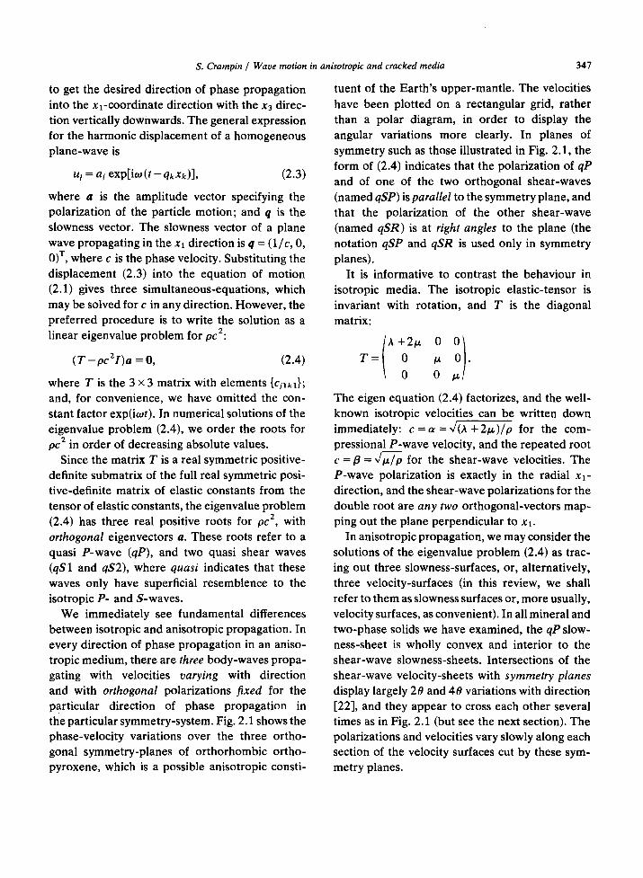
It is informative to contrast the behaviour in isotropic media. The isotropic elastic-tensor is invariant with rotation, and T is the diagonal
T =
matrix:
0 /a, .
0 0
The eigen equation (2.4) factorizes, and the well- known isotropic velocities can be written down immediately: c = a = x/(A + 2 ~ ) / p for the com- pressional P-wave velocity, and the repeated root c =/3 = ~//~/p for the shear-wave velocities. The P-wave polarization is exactly in the radial xl- direction, and the shear-wave polarizations for the double root are any two orthogonal-vectors map- ping out the plane perpendicular to xl.
In anisotropic propagation, we may consider the solutions of the eigenvalue problem (2.4) as trac- ing out three slowness-surfaces, or, alternatively, three velocity-surfaces (in this review, we shall refer to them as slowness surfaces or, more usually, velocity surfaces, as convenient). In all mineral and two-phase solids we have examined, the qP slow- ness-sheet is wholly convex and interior to the shear-wave slowness-sheets. Intersections of the shear-wave velocity-sheets with symmetry planes display largely 20 and 40 variations with direction [22], and they appear to cross each other several times as in Fig. 2.1 (but see the next section). The polarizations and velocities vary slowly along each section of the velocity surfaces cut by these sym- metry planes.

348 S. Crampin / Wave motion in anisotropic and cracked media
a b c X-CUT Y-CUT
9 . 8 9.0 9. Z-CUT
f QP 8.0 8.0 . . . i t
klA ~ / tlA t.d ~ UD tO ~ . 7 . ~ ~ 7 . 0 ~ . 7 . C
Z Z Z
~- 6.0 ~- 6.0 6.0
(_3 L3 c3 E3 E3
_J L~ L~ L~
uJS.0
"----- / / - OSR _ ~ - - , . ~ . . . . _ QSB > z ~ QSP a: >- >- g
o c n q . 0 an Lt.0 clnq.
O 30 60 90 0 30 60 90
8
% QP
QSR
0 30 60 90
Fig. 2.1. Intersection of the phase-velocity surfaces (solid lines) and the wave or group-velocity surfaces (dashed lines) of the three body-waves with the three orthogonal symmetry-planes of orthorhombic orthopyroxene (elastic constants from [41]):
(a) x-cut symmetry plane; angles measured over 90 ° from the y-axis towards z-axis, (b) y-cut symmetry plane; angles from z-axis towards x-axis, and (c) z-cut symmetry plane; angles from x-axis towards y-axis.
The qSP waves are shear-waves with polarizations parallel, and qSR at right angles to each symmetry-plane.
Fig. 2.2 shows just more than a solid octant of
the two shear-wave phase-velocity surfaces for
orthopyroxene. The qP-wave velocity-surface
(not shown), and the two quasi shear-wave
velocity surfaces are almost spherical surfaces with no marked features, apart from the slight
indentations and projections associated with
the shear-wave singularities discussed in the next section.
2.2. S h e a r - w a v e singulari t ies [22, 23, 24]
The behaviour of shear waves in symmetry
planes, such as those shown in Fig. 2.1, appears comparatively straight-forward. This apparent simplicity is misleading. Tracing each shear-wave round the orthogonal corner in Fig. 2.1, the polarizations demonstrate that the two phase-
velocity sheets are analytically continuous: the
shear waves must cross each other an odd number
of times (and at least once) on rounding the corner.
The shear-wave sheets are analytically continuous
in all anisotropic media, and the sheets must come into contact at least twice as the velocities are
unaltered by 180 ° rotation, because of the sym-
metry of the tensor transformations. The points of contact are directions of singularity of the shear-
wave roots. They most commonly occur on planes of mirror symmetry, although they may occur in off-symmetry directions in trigonal, orthorhombic, monoclinic, and triclinic systems. It is surprising that, although singularities in the shear-wave sheets are well known (they are usually called conical points [38]), the essential analytical con- tinuity of the shear-wave sheets does not appear to have been recognised before 1977 [8].

349
-Z -Z QS2
S. Crampin / Wave motion in anisotropic and cracked media
-Z
X
i l
-Z
X
i b
Fig. 2.2. Projections of just more than a solid octant of the phase-velocity and group-velocity surfaces of the shear waves in orthopyroxene projected onto a plane from infinity. (a) projections of the faster sheet qS1, and (b) projections of the slower sheet qS2. The upper octants are of the phase-velocity surfaces, where the arrows mark the positions of point singularities. The lower octants are of the group-velocity of wave surfaces and include three plane sections of the singular feature associated with the singularity near the y
axis.
T h e r e are three types of singulari ty: kiss
singularities, where the two sheets touch t angen-
tially with e i ther convex or concave contac t ; inter-
section singularities, where the two sheets may be
cons ide red as cut t ing each o the r a long a c losed
curve (such in tersect ions are only possible in
systems of hexagona l symmet ry , when the closed
curve is a circle about the symmet ry axis); and
point singularities, where the two sheets have
c o m m o n points at the ver t ices of cone - shaped

350 S. Crampin / Wave motion
projections of the surfaces. Singularities are very common in most systems of anisotropic-symmetry (see Section 7.1, below); in cubic symmetry, for example, which in many ways is one of the simplest of the symmetry systems, the shear-wave phase- velocity surfaces have eight point singularities and six kiss singularities. The orthorhombic system in Fig. 2.1 has point singularities at 14 ° and 70 ° from the y-axis in the x-cut, and at 10 ° from the x-axis in the z-cut. It is very close to a kiss singularity at 55 ° from the z-axis in the y-cut, but the sheets do not quite come into contact.
Shear-wave singularities are well-known fea- tures of propagation in anisotropic solids (Duff [42], for example), but what has only recently been recognised is the effect singularities have on the polarizations of each shear-wave sheet. The behaviour at intersection singularities is simple and obvious. Kiss and point singularities, however, may cause considerable complications to the shear-wave behaviour in neighbouring directio.ns. Fig. 2.3 illustrates the behaviour near the point singularity at 14 ° from the y-axis in the x-cut or thopyroxene of Fig. 2.1. The sections of the two shear-wave velocity surfaces in Fig. 2.3a have point contact in the symmetry plane, but, in off- symmetry directions, the velocity variations pinch together with varying degrees of tightness de- pending on the distance from the singularity. As the direction of propagation passes such a pinch, the polarizations of the two shear-wave sheets are exchanged. Fig. 2.3b demonstrates how the polarization of each shear-wave sheet swings through 90 ° . Such pinches cause only minor modifications to the behaviour of plane shear- waves, but may produce very complicated behaviour in spherical wavefronts and rays from point sources [24].
All shear-wave phase-velocities in all aniso- tropic materials lie on one analytically continuous surface of two sheets [8, 23, 31]. However, for convenience, we shall treat the surface as having two sheets, which touch in a limited number of singular directions. We call the faster sheet qS1, and the slower qS2. Shear waves propagating
in anisotropic and cracked media
( J b J ( f ]
Z
o
b3 >
b3 > (%
Z
g C23 r n
5. a
q.
q.,
°I'x
1o 20
RNGLE FROM T AXIS
30
D 4 ~ ~ ~ , x x
~: ~ \ V , T
t~ 2~ 3O
ANGLE FROM T AX]5
Fig. 2,3. Behaviour of the shear-wave velocity-surfaces near the point singularity at 14 ° from the y-axis in x-cut ortho- pyroxene (Fig. 2.1a):
(a) Sections of the phase-velocity surface. Solid lines are the intersections with the x-cut symmetry-plane, and the lines with increasing length of dash correspond to intersections with planes rotated about the y-axis away from the symmetry plane by 2 °, 5 °, 10 °, 20 °, and 30 °, respectively.
(b) Relative amplitudes of body-wave polarizations of the slower shear-wave, qS2, in the off-symmetry planes in (a), above, relative to the Normal out of the planes of variation, and
the Radial and Transverse directions in these planes.
parallel to symmetry planes, which we have named qSP and qSR, may lie partly on one shear-wave velocity-sheet and partly on the other.
Fig. 2.2 shows the three-dimensional nature of the phenomenon. There are three point-singu- larities, in the solid octant of the phase-velocity sheets illustrated, corresponding to the shear- wave crossings in the plane sections of Fig. 2.1. The singularities are marked by shallow conical

x
Z-CUT
85
70
50
40
Z
X
Z-C
UT
Y
z
Y-C
UT
z
Y-C
UT
85
70
50
40
Y
X-C
UT
"l'
X
-CU
T
Z
z
85
70
50
40
50
4O
50
40
/ 5O
4O
x
Z-CUT
"( -C
UT
T X-CUT ~ Z
3"
g~
g~
¢% &
&
Fig.
2.4
. S
tere
ogra
phic
pro
ject
ions
of
the
phas
e-ve
loci
ty s
urfa
ces
of o
rtho
pyro
xene
ont
o th
e th
ree
sym
met
ry-p
lane
s: t
he z
-, y
-, a
nd x
-cut
s (f
rom
the
top
). O
n th
e le
ft o
f ea
ch s
tere
ogra
m is
the
sect
ion
of y
-, x
-, a
nd z
-cut
s, r
espe
ctiv
ely.
The
con
tour
s ar
e la
bell
ed in
km
/sec
x 1
0, a
nd t
he s
mal
l sol
id c
ircl
es in
the
she
ar-w
ave
ster
eogr
ams
mar
k th
e po
siti
ons
of t
he s
hear
-wav
e si
ngul
arit
ies.
The
ste
reog
ram
s ar
e:
(a)
qP v
eloc
ity,
(b
) fa
ster
qua
si s
hear
-wav
e ve
loci
ty,
qS I,
and
(c
) sl
ower
qua
si s
hear
-wav
e ve
loci
ty,
qS2.
T
he b
ehav
iour
of
the
cont
ours
and
sec
tion
s is
a l
ittl
e bl
urre
d ne
ar s
ome
of t
he s
ingu
lari
ties
. T
his
is d
ue t
o th
e co
arse
ness
of
grid
of
poin
ts u
sed
to o
btai
n th
e gr
aphs
.
b

352 S. Crampin / Wave motion
indentations of the faster sheet qS1, and by shal- low conical projections of the slower sheet qS2. The two sheets are continuous through the singu- larities at the vertices of these shallow cones.
Seismic observations of anisotropy are fre- quently confined to the variations in one plane of the anisotropic medium, as are most obser- vations of anisotropy in the Earth's upper-mantle [9, 10, 21] and crust [19]. Plane sections of the velocity surfaces, as in Fig. 2.1, are adequate for these applications, and indeed for many three- dimensional modelling studies [15]. However, plane sections cannot indicate the true three- dimensional nature of the variations. Fig. 2.4 shows stereographic projections of the variations of three velocity-surfaces of the orthopyroxene of Fig. 2.1, projected onto the three orthogonal symmetry-planes by the techniques of [24]. The variation of the qP surface is straightforward, although not wholly predictable from the sections of the symmetry planes in Fig. 2.1, but the shear- wave velocity-surfaces show unexpectedly complicated patterns caused by the rapid varia- tions in the gradient of the velocities near singularities.
Projections onto generally oriented planes may show very asymmetric stereograms. However, all stereograms for a particular wave-type in any particular anisotropic medium are equivalent under rotation of the axes.
2.3. Group velocities [8, 22, 23, 24]
A further consequence of the variation of velo- city with direction in anisotropic media is that the wave number, which in isotropic propagation is usually a scalar quantity, becomes a vector, re, for both body-wave and surface-wave propagation in anisotropic media. The classic expression for body-wave group-velocity, U = Oto/OK, becomes
U = (&o/OK1, ato/0K2, &o/OK3) T, (2.5)
and energy transport is no longer always parallel to the body-wave phase-propagation vector, even for non-dispersive media, as it would be in isotropic propagation. For phase propagation in the Xl
in anisotropic and cracked media
direction, 0to/bK1 = c, and, if there is no body-wave dispersion, (2.5) becomes
U ~- (c, O0.)/OK2, OW/~K3) T, (2.6)
Thus, in non-dispersive anisotropic media, the energy travels in the propagation direction at the phase velocity c, but, in general, also has a component perpendicular to the propagation vector, so that ] UI I> c. For propagation in a plane of symmetry, x3 = 0 say, symmetry considerations demonstrate that the energy is confined to the symmetry plane and 0( .O/ /0K3 = 0.
The deviation of the group-velocity from the phase-velocity direction has a negligible effect on propagation of body wave in weakly anisotropic material, when Oto/Ox2 and 0to/0K3 are both small [22]. However, the deviation may produce significant effects, including cusps in the shear- wave slowness-surfaces, for propagation in more strongly anisotropic material [23, 24]. The convex nature of the qP slowness-surface, when it is wholly interior to the shear-wave surfaces, pro- hibits cusps in the qP-wave velocity-variations.
The surface traced out by the energy radiated from a point source in a given time, called the wave surface or group-velocity surface, is the envelope of the wave fronts propagating from a point source in a given time [43]. The general expression for the wave surface is easily obtained from this envelope. If r = V(O, d~) is a point on the phase velocity surface in spherical coordinates, the correspond- ing point on the wave surface has Cartesian coordinates [24]
xl =cos(/) cos 0 V - c o s ~b sin 0 dV/dO
-(sin 4~/cos 0) d V/d4~,
x2 =sin tb cos 0 V - s i n 4) sin 0 dV/dO (2.7)
+(cos ~b/cos 0) d V/dth,
x3 =sin 0 V+cos 0 dV/dO.
Note that there is a copying error in [24] and the sign of the third term of x2 is positive.
The intersection of the wave surface with a symmetry plane takes a particularly simple form.

S. Crampin / Wave motion in anisotropic and cracked media
Points on the wave surface have a velocity
U = (V 2 + (dV/dO)2) 1/2, (2.8)
in a direction
= tan- l ( (V sin 0 + (dV/d0) cos 0)
/ ( V cos 0 - ( d V / d 0 ) sin 0)),
(2.9)
where V(O) is the phase velocity in a direction 0 in the symmetry plane. Postma [44] first derived this expression for transversely-isotropic media, but the expression is also valid for group velocity in any anisotropic symmetry-plane. Fig. 2.1 also shows the intersections of the wave surfaces with the three orthogonal symmetry-planes of ortho- pyroxene determined by (2.8) and (2.9).
An alternative expression for group velocity, which is particularly useful for calculation in a uniform anisotropic half-space, is given by Mus- grave [38], which refers parameters to a fixed coordinate system. Musgrave shows that the ele- ments of the group-velocity vector are
3 Ui (½pV) Z 2 2 2 2 = (a k / a k )[(P V - Ak)Oa k/Oni
k=l
+Ct2kOAk/om], (2.10)
for i = 1, 2, 3, where V is phase velocity; nl are direction cosines, and a k are elements of the polarization vector, both referred to the fixed
353
coordinate system specified by the Kelvin- Christoffel equation:
A l - p V 01~ 1 ot~ 2 °1~1°/3 t (ax)
0~1a2 A E - p V 2 O/20~3 [ a2 = 0,
0~10~3 0~20t3 A 3 - 0 " V 2] a3
and Ak and ak are defined by Equation (2.11) at the bot tom of this page.
This treatment of group velocity is the only
occasion in this review when we find it convenient to use direction cosines and refer elastic constants to a fixed coordinate system.
Cusps in wave surfaces are caused by two types of feature on the phase-velocity surfaces (it is convenient to speak of features on the phase- velocity surface causing cusps on the wave surface, since analytically and numerically the wave surface is derived from the phase-velocity surface). The overall curvature of the velocity surface can caus¢ cusps: for example, there are incipient cusps on the qSP curve at 0 ° in x-cut or thopyroxene of Fig. 2.1a, and 90 ° on the qSP curve in Fig. 2.1c. These would be more pronounced if the convex curva- ture of the velocity surface were any greater. The other features causing cusps in wave surfaces are the high local curvatures close to shear-wave singularities.
Fig. 2.2 shows an octant of the two shear wave- surfaces corresponding to the two velocity- surfaces. The uniformity of the phase- velocity surfaces has disappeared completely and
All= A2 A3
O~20t 3
/Cl111 C1212 C1313 C1312
C1212 C2222 C2323 C2223 C1313 C2323 C3333 C3323
1 C1312 C2223 C3323 2(C2233+C2323)
1 C1113 C2312 C3313 2(C33,2"4-C2313)
1 C1112 C2212 C2313 2(C2213"Jf'C2312)
Cl113
C2312
C3313
½(C3312+C2313) ½(C1133+C1313) ½(C1123+C1312)
C2313 |
12n3n,] ½(c,,22+c,2,2)/ 12n,n2/
Equation (2.11), see text.

354 S. Crampin / Wave motion
there is considerable three-dimensional distortion. The overall curvature of the velocity surface leads to cuspidal edges and fins on the slower sheet qS2; we define edges as three-dimensional cuspidal features with one sharp edge, and fins as three- dimensional features with two sharp edges. The qS2 wave-surface in Fig. 2.2 has cuspidal edges running either side of the y = 0 plane from the x axis to midway between the x and z axes, where they each evolve into fins, one of which runs diagonally across the top of the octant. The behaviour of the two-sheeted shear wave-surfaces near shear-wave singularities may be very complicated. The effects of the singularities near the x and z axes appear to be hidden in the complicated behaviour of the cuspidal edges and fins. However, the singularity at about 14 ° from the y axis displays the classic behaviour of point singularities. The faster shear wave-sheet qS1 has an open hole, and there is a corresponding flat inverted-conical lid, resting point-downwards on the slower sheet qS2, which fits exactly into the hole on the faster sheet. The only way of progress- ing from one sheet to the other (and the only way of crossing the open hole) is by a range of phase- propagation directions which pass directly through the singularity, as in the symmetry planes in Fig. 2.1. The wave directions corresponding to neigh-
bouring section of phase propagation go through rapid variations as indicated in Fig. 2.2. In the qS1 sheet the directions skirt round the hole, and in the qS2 sheet the directions follow tight convolutions in the flat inverted-conical lid.
Cuspidal features associated with overall curvature and the features associated with singularities are frequently asymmetrical and irregular, and a great many possible combinations of features exist. These have not yet been classified in any way. Miller and Musgrave [45] first recog- nised the hole and lid phenomenon, although Musgrave makes no direct mention of it in his book [38]. Burridge [46] examines the hole and lid phenomenon for singularities in cubic nickel, and finds that the lid is a plane surface. Although the lid
in anisotropic and cracked media
for or thopyroxene in Fig. 2.2b is certainly a very shallow cone it is not planar.
One feature of energy propagation in aniso- tropic media is unmistakably clear: energy propagation is a three-dimensional phenomenon. Examination of propagation in one plane, even a symmetry plane, may give no indication of the behaviour in neighbouring directions, particularly if there are singularities nearby. Since singularities are very common features of shear-wave velocity surfaces (Table 7.1, below), singular features are common for shear-wave propagation in all aniso- tropic solids, although, for very weakly anisotropic solids, the angular spread of the features may be very small.
We see that the wave surfaces of shear waves are frequently complicated by projecting and over- lapping cuspidal fins and edges. The expressions (2.7)-(2.9) allow shear-wave propagation to be computed in homogeneous anisotropic-media, but propagation in more complicated structures must be interpreted by means of numerical experiments with synthetic seismograms with spherical wave- fronts.
2.4. P-wave polarizations [29]
Analysis of P-wave arrival-times is the major .seismic technique for investigating the structure of the Earth, but is rather insensitive to the smoothly changing angular-variations expected in aniso- tropic structures. The only occasions, when P- wave arrival-times are likely to unambiguously indicate anisotropy, are in the few places where P waves can be observed over many directions in one plane.
One of the main themes of this review is that shear-wave polarization-anomalies appear to be an important diagnostic, which can be used for estimating in situ anisotropy. Unfortunately, shear-wave arrivals are frequently disturbed by the coda of the preceding P-wave and by S to P conversions. It would be much easier to recognise and investigate anisotropy if P-wave polarizations

S. Crampin I Wave motion in anisotropic and cracked media
displayed anomalies. However, [29] shows that, although P-wave polarizations may deviate signi- ficantly from the phase-propagation direction, the apparent deviation of the polarization from the direction of the great circle or ray arrival is small, and is likely to be overlooked. This is because seismic energy travels along the ray path traced by the group-velocity vector, which also deviates from the phase-propagation vector (see the pre- vious Section) in the same direction as the polarization deviation. Fig. 2.5 illustrates sche- matically the behaviour in a symmetry plane, where the phase-propagation, group-velocity, and polarization vectors are coplanar.
/ 3 - 5
RAY OR ~ . C L GBOUP-VELOCIT V J ~
\ <.
¢
Fig. 2.5 (after [29]). Schematic diagram of the deviation of the polarization and group-velocity vectors from the phase-pro- pagation vector. The heavy line is the particle-motion polarization direction. The polarization deviates from the pro- pagation vector by an angle a, and the ray, or group-velocity vector, deviates by/3, giving an apparent polarization deviation
of B - a .
It can be demonstrated algebraically [29] that, for propagation in symmetry planes in the more common anisotropic systems with cubic, hexa- gonal, tetragonal, and orthorhombic symmetry, the deviation of the group-velocity vector is always
355
in the same direction and just exceeds the devia- tion of the polarization vector. The algebra is rather specialized for this review, and the reader is referred to [29] for details. However, it is worth noting that the quantity that controls the size and direction of both deviations is the constant c1121 referred to the local coordinate system (radial, transverse, and vertical to the phase front). This is the off-diagonal element in the T matrix in the eigenvalue equation (2.4) for the body-wave phase-velocities, when x3 = 0 is a plane of mirror symmetry.
Fig. 2.6 gives some numerical examples of polarization and group-velocity deviations in symmetry planes in alpha-quartz, rutile, and orthopyroxene, showing a range of velocity varia- tions. The deviations of the P-wave polarizations from the phase-propagation direction may be large (up to nearly 30 ° in the strong anisotropy in Fig. 2.6a). However, Fig. 2.6 and numerical examination of a variety of symmetry planes in all symmetry systems shows that the group-velocity deviation is almost the same as the polarization deviation so that the apparent deviation, the difference between them, is small, and likely to be attributed to noise or local heterogeneities. Note from Fig. 2.6a that the deviation of the group velocity is only invariably greater than the polarization deviation for one of three mutually- orthogonal symmetry planes.
Algebraic analysis of group-velocity and polarization deviations has not yet been attempted for general directions of propagation, but numerical examination of a large number of solids from different symmetry systems always indicates almost the same deviations for group-velocity and polarization deviations. Fig. 2.7 shows stereo- grams of the horizontal projections of the apparent P-wave polarizations in anisotropic halfspaces made of the same materials and having the same surface cuts as in Fig. 2.6. In all cases, the horizon- tal projections of the polarizations are nearly radial, and are unlikely to be identified in obser- vations.

356 S. Crampin / Wave motion in anisotropic and cracked media
8.0
S .~ 7.o 7- / ...J u . l
> 5 . B O 30 60 • 90 120
W 3o.o ,=, C3
o.o o =
~= -3a .o ,>, o C3
10.0
. ¢ "
u u J > 7.B
15~ 180 0 38 6°
38 60 90 120 150 180 ANGLE FROM Z AXIS
90
----..% 8 30 60 90
=~ 3o.o 3 o . e _ _
= ~ - ~'~X~ ~ 0.0
"~ -30.0 ~ -30.0 ~- 0 30 60 90 0 30 60 90
C:] ANGLE FROM X RXI5 ANGLE FROM X RXI$
Fig. 2.6 (after [29]). Variation with direction of the qP-wave velocity and deviations of the polarization and group-velocity vectors in planes of mirror symmetry.
Top figures: Velocity variations. Dot ted lines are the phase-velocity variation, and solid lines are the apparent velocity (the group velocity) plotted in the direction of the ray. Lines join corresponding points at every 10 ° of phase-velocity variation.
Bottom figures: Angular deviations. Dot ted lines are the deviation of the polarization, and dashed lines are the d~viation of the group velocity, both plotted against the direction of the phase-propagat ion vector. Solid lines are the apparent deviation of the polarization, the difference of the two deviations, plotted in the direction of the ray. Lines join corresponding points at every 10 ° of phase-velocity variation.
The variations are: (a) x-cut a lpha-quar tz (trigonal symmetry) , (b) z-cut rutile (tetragonal symmetry), (c) z-cut or thopyroxene (orthorhombic symmetry) (Solids are specified in [22]).
N I \
"~"---"- \ I I
/ / xkX\ \
/ . / . I . t ~ ---.'~ \
/ / \ x / / / / / / I t \ ' i
/ I t
N / / /
/ / / i
\ \
N I / /
/ / / / I / 1 - / . _ . . . I
I
\ \ ~ ' - / . / / / \ \ \
" " ~ \ / / / I \ \
a b c
Fig. 2.7 (after [29]). Stereograms of the horizontal projections of the apparent qP-wave polarizations for propagation from a point source in an anisotropic halfspace made of the same materials and having the same surface cuts as in Fig. 2.6. The polarizations are
plotted at equal azimuthal intervals of phase propagation. (a), (b), and (c) correspond to Figs. 2.6a, b, and c, respectively.
3. Matrix formulations tor multilayered media
This section provides basic matrix-formulations, which are the tools for solving many problems in body- and surface-wave calculations in anisotropic
layered-media. We consider an m layered half- space, with the axes, and the layer and interface numbering arranged as in Fig. 3.1. The direction of the apparent velocity c along the surface is confined to the xl direction, and all the elastic

S. Crampin / Wave motion in anisotropic and cracked media
X_ ) X1 i b
1 2
2
M-I M.
M X3
Fig. 3.1. Coordinate axes for multilayered models. Elastic tensors are rotated so that the anisotropic axes coincide with the space coordinates and the apparent velocity along the surface is
in the xl direction.
tensors are rotated accordingly. Since most of the analysis in this section involves complex quan- tities, the distinction between homogeneous and inhomogeneous waves is unimportant for analy- tical and programming manipulations.
3.1. Slowness equations [1, 8, 17, 18]
The general displacement in any of the layers consists of six waves, three travelling upwards (in the direction of negative x3), and three travelling downwards. The displacement can be written as (2.3):
6 Ui= ~ f#ai(n) exp[ito(t--qk(n)xk)], (3.1)
n = l
where f is the vector of excitation functions for the six waves. We take q~ = 1/c, q2 = 0, and p, = cq3(n) for propagation in the xl direction.
The problem is to determine p, for each wave in each layer for a given horizontal phase velocity c. Substituting (3.1) into the equations of motion (2.1), we obtain three simultaneous equations for each layer:
Fjkak = 0, (3.2)
where F#~ 2 =--pc ~$im+Cikmnqkqn; and we have omitted the common factor exp(itot). This can be written as a matrix equation for p (dropping the suffix on p,), frequently called the slowness equation:
Fa = (Rp 2 + Sp + T - pc2I)a = O, (3.3)
357
where R, V, and T are the 3 x 3 matrices {Ci3k3}, {Cilk3}, and {Cjlkl}, respectively: S = V + VT; and I is the 3 x 3 identity matrix. Since R is non-singular, (3.3) can be written in partitioned matrices as a linear eigenvalue problem for p:
[ [ - R - 1 S --R-z~"~ / l 0 ap 0 } - P ~ 0 / ) ] ( a ) = 0 (3.4)
where T = T - p c 2 L The matrix decomposition of the full 9 ×9 elastic tensor into the 3 x 3 sub- matrices R, S, T, and V was originally due to Stroh [47], but has been developed independently by Taylor [17, 18], and has great advantages both for body-wave, and, particularly, surface-wave calculations.
The linear eigenvalue problem (3.4) is suitable for numerical solution, but we continue the analy- sis to demonstrate further computational advan- tages for the next Section. Expression (3.4) can be written in the purely-matrix form:
- R - ' S - R - ' 7 " A P
i o ) ( 7
where if the column eigenvector corresponding to Pi is (a~pi, aT) T, then
P = diag(pl, P2, P3),
/$ = diag(p4, Ps, P6),
A = (al, a2, a3),
= (a,, a5, a6).
The form corresponding to (3.5) for the row eigenvectors of (3.3) is:
pATR - A T 2 r ) ( - R / - 1 S - R 0 - 1 T ) = ~6,iTR -i iTt
_(0 ~ j \~,~TR _t~TT]. (3.6)
The row and column vectors for distinct eigen- values are orthogonal in an n × n linear eigenvalue

358
problem, and, providing a set of n independent column vectors can be found, there exists an orthogonal set of n row vectors, even when the pj are not distinct. Consequently, the product of the row and column vectors is a diagonal matrix. We have
pATR -AT~'~I(Ap At 5
P, U R A 7, J=
= diag(yl, y 2 , . . . , y6), (3.7)
and the matrix of column vectors is the inverse of the matrix of row vectors, if the ai are scaled so that 39 = 1, j = 1, 2 . . . . 6. Since the matrix of row eigenvectors may be constructed from the column eigenvectors:
$. Crampin / Wave motion in anisotropic and cracked media
and the subscript n refers to values in the n th layer. Similarly, the displacement-stress vector at the (n + l ) t h interface is related to the excitation vector of the nth layer by:
pATR - A T ~ p~TR -.~TTJ =
we can obtain the inverse without numerical inversion. Taylor [18] discusses these equations in more detail.
3.2. Propagator matrices [1, 8, 17, 18]
The boundary conditions across any internal welded-interface of the multilayered halfspace are the continuity of the displacements u, given by (3.1), and the continuity of the stresses normal to the interface tr~3, o':s, and o'33, where the stresses are given by
Orik = CtkmnU . . . . (3.9)
The displacement-stress vector at the n th interface is related to the excitation vector ( f ) , in the nth layer by the expression
( . ~ . ) = E , ( [ ) , , (3.10)
where
7" ---- ( i c / t o ) ( o ' 1 3 , 0"23 , or33)T;
I ] ( A P AP E°=( ° V , \ A (3.11)
= E . D . ( [ ) . , (3.12)
where
D, =diag[exp(-iwpfl,/c)], j = 1, 2 . . . . 6;
and dn is the thickness of the nth layer. Combining the expressions (3.10) and (3.11)
we have a propagator matrix (Gilbert and Backus [48]):
'T n + l n'
where G,=E,,D,E~ ~, which allows the dis- placement-stress vector at any interface to be related to that at any other interface by the product of appropriate Gj for the intervening layers.
We now scale aj so that yj = 1 in (3.7), and use (3.7) and (3.8) to obtain
~ z ~ P ~ T ( - v I E : ' = ( A P A } \ - T 0)" (3.14)
Thus the solution of the slowness equation in the form of the eigenvalue problem (3.4), and simple scaling of the eigenvectors at, allows us to construct the propagator matrices without numerical inver- sion of 6 x 6 double-length complex-matrices. This gives considerable savings in computer time, particularly in surface-wave calculations, where the propagator matrices are calculated within iterative cycles (see Section 5, below).
There are a number of new developments in the theory of surface waves in anisotropic media, which have come from the theory of dislocations in solid-state physics. These lead to an alternative, and in some ways more attractive, technique for deriving the inverse of E , without numerical inversion. The technique requires quite different analysis from that reviewed here, and we shall not

S. Crampin / Wave motion in anisotropic and cracked media
describe it as, in its present stage of development, it is much less convenient for describing the range of body- and surface-wave applications we shall discuss in this paper. Chadwick and Smith [49] give a comprehensive review of these developments.
3.3. Matr ix formulat ions }:or piezoelectric
media [17]
Taylor and Crampin [17] demonstrate that the matrix formulations for elastic anisotropy may be extended to include piezoelectric anisotropy. Here, we briefly indicate how the formulae of the previous two sections carry over into piezoelec- tricity; [3, 4, 17] contain details and applications. Volume 2 of Wave Electronics (1976) contains several review papers on Surface Acoustic Wave (SAW) Devices in piezoelectric media, including a
genera l review by Farnell [50]. The equations of motion in a piezoelectric
anisotropic solid, with negligible conductivity, are [51]:
pU] - ~ - CikmnUm.kn "[" ekp,,r~.k~,
for ] = 1, 2, 3, (3.15)
eikmUk,jra -- ~ im~, im = O,
where 4) is the electric potential, and ekp, and el,, are the constants of the piezoelectric and dielectric tensors, respectively.
The elements of the tensors have the following symmetry relationships [52]:
Cjkran = Ckjran = Cmnjk,
eik, ,= ei,,k, and
¢k,, = emk. (3.16)
These symmetries are preserved if we contract the notation by extending cikm, so that subscripts run from 1 to 4, as follows:
C4kmn = ekmn ; C 4 k 4 n = --~kn ;
C44mn ~- C 4 4 4 n = C 4 4 4 4 = O ,
f o r k , m , n = l , 2 , 3 . (3.17)
359
The equations of motion (3.15) can then be written
puj = Cjk,,,.U,,,.k,,, for j = 1, 2, 3, (3.18)
C4kranUm,kn = 0
where u4 = 4); and the implicit summations now run from 1 to 4. The tensor transformation (2.2), for rotating to a new coordinate system (x~), is preserved, with summation subscripts again run-
t X t ning from 1 to 4, and x], 4 - - ~ 4 , ] ----- 0 for J # 4, and x~,4 = 1.
The equations in Sections 3.1 and 3.2 can now be extended with a few minor changes. The dis- placements (3.1) become
8
ui = • fnaj (n)exp[ i to( t - -qk(n)Xk)] , n=l
for j = l , 2, 3, 4 and k = l , 2 ,3 . (3.19)
Substituting (3.19) into the equations of motion (3.18) gives four simultaneous equations:
Fj,,a,, = 0, for j = 1, 2, 3, 4, (3.20)
2 A ^ where F/m = - p c 8jr~ +Cjkm,qkq, and 8j,, is the modified Kronecker function 8i,- = 8jm, for ], m < 4, and 8i,- = 0, when either j or m = 4. The slow- ness equation (3.3) becomes
2 ^ F a = ( R p 2 + $ p + T - p c I ) a =0 , (3.21)
where R, S, and T are defined as for (3.3) with subscripts now running from 1 to 4; and/~ = diag(1, 1, 1, 0). The remaining equations in Sections 3.1 and 3.2 ((3.4) to (3.14)), and many equations throughout this review, extend directly to piezo- electric propagation with subscripts running from 1 to 3, 1 to 4, or 1 to 8, as appropriate.
The application of these piezoelectric equations follows very much as we shall demonstrate, below, for elastic anisotropy. The major difference is that there is now a free-surface boundary-condition for the electric potential. The two cases of most inter- est are when there is a shorting interface and ~b = 0 at z = 0; and when the surface is free and d~ is continuous but decays to zero at large distances from the surface. Both these conditions can be accommodated. A program for calculating the

360
properties of micro-acoustic surface-waves in multilayered piezoelectric-structures has been described in [3, 4].
S. Crampin / Wave motion in anisotropic and cracked media
4. Synthetic body-wave seismograms
The calculation of synthetic seismograms is one of the major techniques for the interpretation of wave propagation. Numerical experimentation allows realistic interpretation of observations from complicated structures, that would have been quite impossible a few years ago. Even in the largely theoretical developments reviewed here, synthetic seismograms and numerical experimen- tation have been a major aid to understanding wave propagation in anisotropic media.
The separation of the phase- and group-velocity vectors in anisotropic body-wave propagation means that the propagation of waves depends critically on whether the waves have plane or curved (we shall call them spherical) wavefronts. Synthetic seismograms of plane waves through plane-layered anisotropic-media are compara- tively simple to compute, but have limited appli- cation to a few very-specific problems. Within these limitations, plane waves have made import- ant contributions to our understanding of aniso- tropic body-wave propagation, and, in particular, they have demonstrated the significance of shear- wave polarization-anomalies for recognising and estimating anisotropy. The next Section reviews applications of plane waves to some simple aniso- tropic structures.
Almost all realistic problems require finite seismic-sources, and the modelling of spherical wavefronts. There are, at present, two principal techniques (with a great many variations) for computing synthetic seismograms with spherical wavefronts in isotropic media. These are the reflectivity method [53, 54] and the ray method [55, 56]. The reflectivity technique, for calculating synthetic seismograms in plane uniform aniso- tropic layers, is particularly suited to the analysis reviewed in Sections 2 and 3 as it makes direct use
of the anisotropic propagator-matrices (3.13). Section 4.2 gives an outline of the method. The ray method is more suited to calculating propagation in continuously varying media. This technique requires rather different analysis, and has not yet been programmed by the reviewer; however, Cerven~, and his colleagues have written several papers on anisotropic ray calculations. One of the problems in the anisotropic ray method is how to specify and attach meaning to varying anisotropic media, where a number of elastic constants vary in space. We shall leave this question until we have a better understanding of anisotropic structures. However, for completeness, we give an outline of the anisotropic ray-method in Section 4.3.
4.1. Plane waves [11, 12, 13, 15]
A plane body-wave of frequency w impinging from a homogeneous halfspace onto a multi- layered structure (Fig. 3.1) may be modelled immediately by the formalism of Section 3. The displacement of the incident wave, of whatever type, qP, q S l , or qS2, may be written as one of the components of expression (3.1):
uj = a i exp[ko (t - Xl/C - x 3 p / c ) ] ,
for] = 1, 2, 3, (4.1)
where c is the apparent velocity in the Xl direction; and p / c = q3 is the slowness in the x3 direction. In an isotropic halfspace, p can be written explicitly as a function of the incidence angle and the constant isotropic velocity a, or/3, as appropriate, but for an anisotropic halfspace, p is one of the eigenvalues of the slowness equation (3.4). Both a and p are real for a non-attenuating homogeneous wave, and p is negative for an upward propagating wave with the axes in Fig. 3.1.
The displacement-stress vector at the top sur- face of the homogeneous halfspace can be written (3.10)

S. Crampin / Wave motion
where (Jr),, = (fl , f2 . . . . . f6) T is the excitation vector in the halfspace. We order the pj in Em so that [j = t~jk for j = 1, 2, 3, where k = 1, 2, or 3, for the appropriate incident qP, qS1, or qS2 wave, respectively, and the fj, for j = 4, 5, 6, are the excitations of the three downward-propagat ing waves.
The product of propagator matrices (3.13) relates the displacement-stress vectors at the top of the halfspace to those at any other interface. The solution is determined by relating the half- space vector to the boundary conditions at the free surface, where the components of normal stress vanish. We have
(8,k, 82k, 83k, / , , fs, f6)~ =
= E ~ I G ( u l , u2, u3, O, O, O) T, (4.3)
1 where O =I - [ .= . , - t O. f rom (3.13); and u is the displacement vector at the surface. The wave motion throughout the layered structure is com- pletely specified by the apparent velocity c of the given incident wave.
Many details of plane-wave propagation, including synthetic seismograms, can be obtained directly f rom (4.3). Synthetic seismograms are determined by convolving the product of the complex spectrum of the incident pulse with f requency-dependent transfer-functions derived f rom (4.3).
The behaviour of the energy propagat ion of plane waves may be calculated by using the expressions for the energy-flux vector, F~, of Synge [57]. The elements of the flux vector, for both homogeneous and inhomogeneous waves, are [11 ]
1 2 , :g F 1 ='&tO f f Cikmn(akqma n +akq*ma* n),
for j = 1, 2, 3, (4.4)
where f is the vector of excitation functions; and the asterisk denotes the complex conjugate. Vectors q and a are both real for homogeneous non-at tenuat ing waves, and (4.4) reduces to
F j ~ _ ~ 1 2 t t , ~to f! Cikmnakqma, ~. (4.5)
in anisotropic and cracked media 361
In isotropic media (4.5) becomes
1 2 , F i =-~to f f (A +2g,)qi
for P waves, and
Fj = ½to2 f f * p.q,
for shear waves. The three plane body-waves propagat ing in the
same direction are orthogonaUy-polarized, and the polarizations are not, in general, radial or transverse to the propagat ion direction [8]. These polarizations cause phase conversions at inter- faces: the anomalous conversions between qP and the quasi shear-waves are usually small, because
the qP wave is nearly radially polar- ized; but the behaviour of the two shear-waves causes anomalies at most isotropic/anisotropic interfaces.
The wavefront of a plane wave is of infinite extent and possesses infinite energy. This severely limits the realism of most models. However , Crampin [15] demonstra ted some aspects of anisotropic wave-mot ion by the propagat ion of plane waves at normal incidence through the vertical slab of anisotropic material set in an isotropic solid shown in Fig. 4.1. The velocity
x x x
x " " x x
x x x '~x
x x Z , , \ x
/ \ , " , xx'~ \ x
x x
(jR DIRECTION OF PROPAGATION
%%
%%
Fig. 4.1. Structural model for synthetic seismograms: an iso- tropic solid (p = 2.6 gm/cm 3, a = 5.8 kin/see, /3 = 3.349 km/sec) with an anisotropic slab-shaped volume (the anisotropy simulating distributions of aligned cracks) posi- tioned normal to the propagation vector. The orientation of the anisotropy is specified for the initial orientation (top three- component trace in Fig. 4.3), and is then rotated successively by
22.5 ° about the vertical (Z) axis to give five orientations.

362 S. Crampin / Wave motion in anisotropic and cracked media
8.0
5.S / QP
,/
,.° / /
S.5 J
S . E
/ f gP
.d ~: tl..C ~ (~ tl.O ~ z (~Z Z O Z ( . - ) Z
~ m --. . = ~ ' q . ~ I t
tlJ Z ~ . 5 II Z 3,~ = ~ G ~ ' - ;= - - C~ • > . -
C~ I,U ~ N , == ,~=~
NN g~..~ NN Na.s
Q$P
30 BO 90
g ~
;a
= d
6 . 8
5.~
tt,5
w~ tt'(3.~
z 3 . 5
,T, >3,0, .
~2.S 3g
QP
68 90
QSR
QSP
Fig. 4.2 (after [15]). Phase velocity variations through cracked solids for angles of incidence between 0 ° (normal) and 90 ° (tangential) to a distribution of thin parallel-cracks (solid lines), and through purely-elastic anisotropic-solids with similar velocities (dashed lines). The parameters of the isotropic solid are given 'in the caption to Fig. 4.1.
(a) GKFF1; dry cracks with crack density E = 0.1, (b) GKFF6; dry cracks w i t h , = 0.025, and (c) G K L F I ; saturated cracks with E = 0.1.
variations of the materials within the slab are illustrated by the dashed lines in Fig. 4.2. These materials are purely-elastic solids with hexagonal symmetry simulating the velocity variations (solid lines) of thin parallel-cracks in an isotropic solid [15] (the modelling of cracked structures is dis- cussed in Section 9.2, below). Figs. 4.2a and 4.2b model two distributions of dry cracks with different crack densities, and Fig. 4.2c models a distribution of liquid-filled cracks.
We shall not illustrate P-wave propagation here as the anomalies are small (but see [15]). Fig. 4.3 show synthetic seismograms of plane shear-waves incident from the isotropic solid and propagating through the anisotropic slabs for five orientations
of the anisotropy. The orientations of the aniso- tropy in Fig. 4.3a is arranged so that the fixed polarizations of the shear waves in the direction of propagation coincides with the polarizations of the seismograms. This is clearly demonstrated in the polarization diagrams in Fig. 4.4a, where the particle motion is displayed in orthogonal sections for successive time-intervals along the seismo- gram. The shear waves split on entering the aniso- tropy into components with fixed polarizations (in this case, SH, and SV, polarized parallel to the T and Z axes, respectively), which are separated and clearly visible on the unprocessed seismograms. These two orthogonally-polarized quasi shear- waves propagate at different velocities, so that on

$. Crampin / Wave motion
leaving the anisotropy the incident wave-form cannot be reconstituted.
The anisotropic material of the slab in the model used for Fig. 4.3b is oriented so that the fixed polarizations are not parallel to the components of the seismogram. This is likely to be the situation for most observations of seismic waves through anisotropic media. The incident shear-wave splits, as before, and separates into two orthogonal pulses, but this is not immediately obvious from the (unrotated) seismograms. However, the split- ting is clearly seen as cruciform patterns in the polarization diagrams in Fig. 4.4b.
Observed seismograms usually show shear wavetrains with several cycles of motion, and the two orthogonally-polarized wavetrains will over- lap after the initial delay. In such cases, polariza- tion diagrams do not show cruciform patterns, but have abrupt changes from linear to elliptical particle-motion. The polarization diagrams in Fig. 4.4c for the seismograms in Fig. 4.3c demonstrate these abrupt changes in particle-motion direction, where the two shear-wave pulses overlap. Such abrupt changes of direction in polarization diagrams are strongly diagnostic of anisotropy. Similar anomalies have been observed in shear waves propagating through earthquake source regions [26], and are believed to indicate aniso- tropy caused by extended dilatancy--the opening of existing cracks in stressed rock.
These seismograms in Fig. 4.4c are for a model with much weaker anisotropy than in the other two figures, and show an interesting effect. The delay between the two split shear-waves, after passing through the anisotropy, is approximately half the dominant period of the pulse (or the length of the anisotropic path is half the dominant wavelength), and the effective polarization of the incident shear- wave is changed by 90 ° by passage through the anisotropy. This phenomenon is caused by the constructive and destructive interference of the two orthogonally-polarized waves from the decomposition of the original incident pulse. If the incident shear-waves were a nearly harmonic wavetrain lasting several cycles, as is frequently
in anisotropic and cracked media 363
the case for many shear arrivals in the Earth, the constructive and destructive interference through an appropriate anisotropic region could result in a much larger transfer of energy from one polariza- tion to another.
The small P-wave components arriving before the main shear-wave arrivals in Fig. 4.3 are from S to P conversions at the entry and exiting inter- faces, and indicate that the seismograms in Fig. 4.3a were calculated for a receiver (10 km) beyond the slab, and that those in Figs. 4.3b and 4.3c were calculated for the exiting interface of the slab. These S to P conversions are very much modified by the nature of the interface between the isotropy and the anisotropy, and would disappear if there were a transition zone. The behaviour of the split shear-waves, however, is not very sensitive to the nature of the interface between the isotropy and the anisotropy, and, in particular, it is not very sensitive to whether the change to anisotropy is discontinuous or whether there is a transition zone. Crampin [15] discusses and illustrates the phenomena in Figs. 4.3 and 4.4 in more detail.
4.2. Spherical wavefronts by the reflectivity method [27]
The reflectivity technique for synthetic seis- mograms was originally developed [53, 54] to calculate spherical wavefronts from explosive sources at the surface of a plane-layered isotropic- model (as in Fig. 3.1). The waves reflected and refracted from the layers are evaluated, again on the surface, at a number of points to form a record section modelling observations from deep reflection and refraction surveys. The technique is particularly valuable for interpretation as it can demonstrate arrivals, phases, and amplitudes, which otherwise could not be easily estimated. The presence of anisotropy in the continental uppermantle [58, 59] was the original motiva- tion for developing an anisotropic reflectivity- method [27].

364 S. Crampin / Wave motion in anisotropic and cracked media
a I ,I ~1 31
a .~
T
R
T
t SEC
S HZ Sq5 NRVE THROUGH
LF1 RT 5 0 R I E N T N S ,
i ,i 21
-'r
Z
T
1 SEC
5 HZ SH NRVE THROUGH
TILTED FFI f i t S ORIENTNS.
C
Z .
R
T
I ,J 21
z i R _ _
T
T ~ V - -
R L
1 SEE
S HZ SV ~JRVE THROUGH
FF6 T ILTED RT S ORIENTNS.
Fig. 4.3 (after [15]). Synthetic seismograms of 5 Hz shear-waves through a 10 km thick slab (Fig. 4.1): (a) •ncident shear-waves with p••arizati•n intermediate between SH and •V pr•pagating thr•ugh a s•ab •f GKLF•• with the initia•
orientation so that the axis of cylindrical symmetry is transverse horizontal (parallel to the T direction in Fig. 4.1). The seismograms are calculated for a position 10 km beyond the slab.
(b) Incident SH-waves propagating through GKFF1, with the initial orientation having the axis of symmetry dipping 45 ° to the transverse direction. Seismograms calculated for the exit interface of the slab.
(c) Incident SV-waves propagating through GKFF6. Orientations as in (b), above.
The procedure for propagation in isotropic
m e d i a is to form a plane-wave decomposition
of a point source, usually in a potential-function representation, as a Sommerfeld integral over
wave number at a given frequency. A variety of
explosion and earthquake source-mechanisms can be specified by wave-type, phase, and amplitude of the plane waves. Each plane-wave is transformed through the various layers in the model structure by using isotropic propagator-matrices [48] to obtain the appropriate reflectivity-coefficients
(plane-wave reflection coefficients) for upward propagating waves in the surface layer. The
reflectivity coefficients are inserted into the plane-
wave representation, evaluated at the required
distance along the surface, and then integrated
twice: once over the appropriate range of wave numbers (apparent velocities) to obtain the spher-
ical wavefront; and finally convolved with the
source spectrum to give the synthetic seismogram at the specified distance from the source.
The procedure for anisotropic propagation is similar in broad outline, but differs considerably in
detail: for example, the three-component coupling that is such a distinctive feature of anisotropic propagation requires that all three components of motion are calculated simultaneously, instead of separating the P and S V , and the independent S H

S. Crampin / Wave motion in anisotropic and cracked media 365
I 2 3
O 0 O 0 O t
R ilL" " "~
0 tO O 1
U O U
- - d " . . . . "G . . . . . u - -
O 1o O 10 0 l
- - ~ I0 o to o 1
O 0 O t
[ ~ 0 0 0 t
1 2
o 0 D 1 V U
D 0 D 1
U U
O tO 0 l U U
D lO D 1
U V
O tl 0 t
U U
0 ~ O t
U V
T R
U U
0 1~ 0 t
u v
D 0 D I
O U
0 ~ C t
a b
I 2
T RT R
O 0 D I
U U
D tO 0 l V U
O !0 O 1
T I e R T R
0 10 n 1
L RL R
O lO D 1
T AT A
0 tO 0 1
0 I0 O t
U !
0 l0 !
O l0 1
Fig. 4.4 (after [15]). Polarization diagrams: cross sections of the particle motion, for the numbered time intervals above the synthetic se ismograms in Fig. 4.3, with directions Up, Down, and Towards and Away from the source, and U, D, and Left and Right facing the source (the Z axis is vertical). Five sets of diagrams correspond to the five sets of se ismograms in Fig. 4.3 for (a), (b), and (c),
respectively.

366
calculations, as in isotropic propagation. We assume, for the sake of simplicity, that the source is in a layer of isotropic material. In the notation of Section 3, the excitation vector in the top layer (label 1) containing the sources is related to the excitation vector in the halfspace (label m) by
( f l , f2 , f3 , O, O, O)Tm =
= K(3'l, 3'2, 3"3, f4, fs, f6) T, (4.6)
where the first three elements of the excitation vectors are downward, and the last three upward propagating qP-, q S l - , qS2-waves (if the layer is anisotropic), or P-, SH- , and SV-waves (if the layer is isotropic), respectively;
K = E~IEm_IDm-IE~I -1 . • . E1D1
in the notation of Section 3.2; and 3'1, 3'2, y3 are the excitations of the downward propagating waves from the source. Equation (4.6) can be solved, for specified yj, for the upward propagating (f)l in the surface layer. These (f)l are the reflectivity coefficients. Thus, by setting yl = 1, and y2 = 3'3 = 0 for a P-wave source, for example, we have
( /4)1 = Re, e, (f5)I = Rp,$H, and (/6)1 = Re, sv, for the reflectivity coefficients in the usual notation [53, 54]. Once the reflectivity coefficients have been determined, the displacements and stresses at the surface can be obtained from
(Ul , U2, U3, 7"13, 7"23, 7"33)T =
= E~(O, O, O, f4, fs, f6)T,
S. Crampin / Wave motion in anisotropic and cracked media
(4.7)
where we have omitted the direct waves from the source. Integrations over wave number and fre- quency then yield the required three-component synthetic seismograms.
The major difficulty of this anisotropic reflectivity-method, as we have outlined it here, is that calculation of several large matrices of reflectivity coefficients is a very lengthy compu- tation, and can frequently result in considerable loss of numerical precision. There are two ways these difficulties can be avoided in isotropic
reflectivity. Kind [60] makes use of the redun- dancy in the isotropic propagator matrices, and manipulates minors of the matrices to produce a faster program which reduces the loss of precision. The direct extension of Kind's technique is not appropriate to the 6 x 6 anisotropic propagator- matrices, and alternative matrix-manipulations have not yet been developed. Kennett [61] develops an iterative technique for calculating isotropic reflectivity-coefficients, which leads to increased accuracy and speed of computation, as well as permitting calculations of synthetic seis- mograms with and without reverberations inclu- ded, which is a valuable interpretative facility. Kennett 's iterative technique can be adapted to anisotropic reflectivity and is used in the program under development [27].
The reflectivity method is very flexible, within the limitation of parallel layering, and can model many different propagation paths by manipulating the basic structure in Fig. 3.1, and by modifying the form of the propagator representation in equa- tions (4.6) and (4.7). Thus we are currently using the anisotropic reflectivity-method to model record sections for deep refraction surveys of anisotropy in the upper mantle, and the propaga- tion from acoustic events through the crack aniso- tropy in hot-dry-rock geothermal-heat reservoirs.
The underlying assumption in the anisotropic reflectivity technique, as set out above, is that the energy radiating from a point source is confined to the sagittal plane. This is wholly true only when there is sagittal symmetry, and, in general, rays will deviate from the sagittal plane. However, in most cases the seismogram will be a good first approx- imation, even without sagittal symmetry. The exact seismogram would require an integration over a vector horizontal-wavenumber K = (K~, K2) T, for a range of directions either side of the sagittal plane. In principle, this is straight- forward, but has not yet been done as it would add considerably to the running time of an already lengthy program, and, in general, would lead to only minor modifications to the seismograms.

S. Crampin / Wave motion in anisotropic and cracked media
4.3. Spherical wavefronts by the ray method [56]
The ray method for tracing ray paths and cal- culating synthetic seismograms with spherical wavefronts, originally proposed by Babich and Alekseev [55], has been extensively developed by (~erven~, Molotkov and P~en~ik [56] and their colleagues in Prague. This brief outline of the technique has been written for this review by Mat Yedlin for which I am very grateful. The many original papers by Babich and (~erven~ should be referred to for details of the method. This is the only part of the anisotropic development reviewed here that has not been investigated numerically by the author.
The equations of motion in a possibly non-
uniform anisotropic media are
aiij = ( Cjkm~U,.,. ).k, (4.8)
where p, Cjkm., and their derivatives are continuous functions of the space coordinate. A solution is sought in the form of a ray expansion:
u(x, t )= ~. u ( " ) ( x ) F . ( t - r ( x ) ) , (4.9) n=O
where the functions u(")(x) are the vector ampli- tude-coefficients of the ray series; r(x) is the phase function or eikonal such that t = r(x) describes the wavefront; and F.(~') satisfies the relationship
F ' F.-I(~) = . (~), where F " (~') = 0F.(~')/0~. Substitution of (4.9) into (4.8) yields several
systems of equations. Equating coefficients of the functions F . yields a system of recurrence rela- tionships for u ("), where U(-1)=U(-2)----0. The lowest order equation
( r k m ° , ~o) - - O k m ) U m = 0 , (4,10)
provides three algebraic equations for u ~°), where Fkm = aik,..qiqn, ajk,.. = Cik.,./P, 8k,. is the Kronecker delta, and q is the slowness vector.
The eigenvalue equation for the matrix Fkm is
( F - G I ) g = O , f o r i = l , 2 ,3 , (4.11)
which has eigen values G~, G2, and G3, and the corresponding eigenvectors g(:), g(2), and g(3) are
367
the polarization vectors of the three body-waves (compare with (2.4)).
Clearly (4.11) has a non-trivial solution only when
G,(x, q)= 1, (4.12)
for i = 1, 2, or 3, corresponding to each of the body waves. Since q is the wavefront normal, (4.12) is a non-linear partial-differential equation defining the propagation of the three wavefronts. The system of ordinary differential equations for the first-order rays can be written as
d x i / d r = ½0GdOqi ,
dqi/ d r = -½0Gi / Ox]. (4.13)
Expressions for the partial derivatives of Gi in (4.6) can be evaluated by implicitly differentiating
det(F - G I ) = 0. (4.14)
The resulting ray-tracing equations are
dxj/ d z = aikm.qnDkm/ D,
dq i /dr 1 = --'~(Oakr,,,,JOxi)qkqpD,,.,/D ,
where
(4.15)
Dl l -- (/'22 - 1)(/'33 - 1 ) - F23,
D12 = D21 = -/'13F23 - -F'I2(-F'33 - 1)
022 = ( / ' 1 1 - 1 ) ( r 3 3 - 1 ) - r h ,
D13 = D31 = r12F23 - r13(r22 - 1),
D33 --- (Ell - 1)(]"22 - 1 ) - F22,
D23 ---D32 --- F12/'31 -F23(F11 - 1),
and the trace D = D l l + D 2 2 + D a a .
Cerven# et al. [56] show that synthetic seis- mograms are the sum of the elementary seis- mograms u ("), which may be obtained from the above equations, when the wave type has been specified at the source. There are a variety of numerical methods for solving these equations. An increasingly popular method for the solution is by implicit finite-differences when the source- receiver offset has been specified [62].

368 s. Crampin / Wave motion
These various ray-techniques work unambig- uously for qP waves and for quasi shear-waves, when the eigen values of (4.11) are distinct; that is D ~ 0 in (4.15). However, we have seen in Section 2.2 that quasi shear-waves have singularities, with identical eigenvalues, for several directions of propagation in every anisotropic solid. The velo- city and polarizations of the quasi shear-waves vary slowly along any path that takes the waves through a singularity, i f the path lies in a symmetry plane. The seismograms and ray tracings for such paths will display no unusual features, even though the waves will have passed from one to the other of the slowness sheets of the analytically continuous shear-wave slowness surface.
The situation will be quite different for shear waves whose path comes close to the direction of a point singularity, say, but does not pass through the singularity (the other types of singularity will have similar effects). Along such a path, l~he polarizations of each shear-wave will change by nearly 90 ° for a very small change in the direction of propagation (see Fig. 2.2b). The physical effects of this phenomenon will be to transfer energy continuously to the other slowness sheet while the polarizations are varying, and energy will be radi- ated (diffracted) in a comparatively wide, but limited, range of directions. In some circum- stances, almost all the energy will be transferred from one sheet to the other. We do not know how this behaviour can be incorporated into the ray method without rather unsatisfactory approxima- tions. One such approximation would be to divide the structure into very fine, but discrete, layers near the point where the wave is passing near the direction of the singularity. Since the polarization may change rapidly over very small changes in direction, these subdivisions would need to be very fine indeed.
Such problems involving singularities only arise in continuously varying media, and do not occur in the reflectivity method, which has been suggested in Section 4.2, for modelling propagation through discrete uniform-layers.
in anisotropic and cracked media
5. Surface waves in a multilayered haltspace
The calculation of surface-wave dispersion in plane-layered structures has played a major part in analysing isotropic Earth structure for over 20 years (sometimes with an approximation cor- recting for the curvature of the Earth at long wavelengths). The effects on surface waves of anisotropy in the Earth's upper-mantle, although suspected for sometime [63], have only recently been confirmed both for continental [10] and oceanic [21, 64] paths, and appropriate compu- tational procedures have been developed [10, 20]. A parallel, although largely independent, develop- ment with extensive literature has been the cal- culation of surface waves in unlayered or single- layered piezoelectric halfspaces for surface- acoustic-wave devices in the electronic industry [50].
Isotropic calculations have now reached a high degree of sophistication based on various matrix- manipulations [65] not available for anisotropic calculations. Crampin [1] originally proposed a simple extension of the Thompson-Haskell iso- tropic-matrix formulation [66] to anisotropic multilayered halfspaces. A significant improve- ment to the formulation since [1] has been the decomposition of the full 3 x 3 x 3 × 3 elastic- tensor into the 3 × 3 submatrices of (3.3) [17, 18].
Surface waves in anisotropic media have some distinctive differences from propagation in iso- tropic" media, although the difference between single-component seismograms from anisotropic and isotropic media may be subtle and easily over- looked. The two independent families of isotropic
Rayleigh-modes and Love-modes coalesce in anisotropic media into one family of Generalized modes propagating with elliptical particle-motion in three dimensions [1, 5]. In structures with weak anisotropy, alternate modes usually correspond to isotropic Rayleigh- and Love-mode particle- motion, although only in directions of sagittal symmetry do the Generalized waves have strictly Rayleigh- or Love-type particle-motion. The polarization anomalies caused by this three-

S. Crampin / Wave motion in anisotropic and cracked media 369
dimensional particle-motion are the most distinctive recognisable features of anisotropic surface-wave propagation.
The problem in surface-wave calculations is to determine the phase velocity at a given frequency (or frequency at a given phase velocity) for any particular mode. The search procedure for multi- layered models is usually an iterative trial and error technique. Once this dispersion relationship has been found, all the other parameters of the propagation, with the exception of the group velocity, can be determined by direct substitution in the appropriate equations. Group velocity in anisotropic media cannot be directly determined from the equations, as it can for isotropic media [65], but must be calculated either from (2.5) by differentiating the phase velocity with respect to frequency and direction of propagation [2], or from integration of the energy flux over depth [57].
The formalism of Section 3 applies throughout.
5.1. Solid surface-layer [1, 2, 5, 8, 10]
The boundary conditions at the free surface of a solid multilayered-halfspace (Fig. 3.1) are the vanishing of the normal stresses, and the radiation condition for normal-mode propagation is that there are no waves propagating upwards in the homogeneous halfspace. In the notation of Section 3, the conditions at the free surface and in the lower halfspace are related by
T (o,o,o,f.,f~,f~).,=
=E~,IG(ul, u2, u3, 0, 0, 0)1 T, (5.1)
where f4, ]5, [6 are the excitation functions of the three downward propagating waves in the half- space; E,, is the E matrix (3.11) for the halfspace; G is the product of the propagator matrices (3.13) for the intermediate layers; and (u)l is the dis- placement vector at the free surface.
A non-trivial solution to (5.1) exists only if
det(J) = 0, (5.2)
where, if matrix K = E~IG has elements {kik}, for ] , k = l , 2 . . . . 6,
/ k l l k12 k131 J= ~ k2, k22 k23~.
\k31 k32 k33/
(5.3)
Equation (5.2) can be solved by recalculating matrix K, for different values of frequency and velocity c, until the position of the determinant zero can be estimated [2].
Solutions have been calculated for a variety of isotropic structures with internal anisotropic- layers modelling anisotropy in the upper mantle of the Earth. It is clear that different structures can show a very wide range of phenomena, and the following comments are drawn from this limited sample of calculations modelling Earth structures, whose major feature is a low-velocity crust over a high-velocity mantle at a depth of about 30 km beneath continents and about 8 km beneath oceans.
The dispersion of any single anisotropic-mode of propagation can usually be modelled reasonably well over a comparatively wide frequency-band by an equivalent isotropic-structure. Thus inversion, for structure, of the dispersion of a single mode alone is unlikely to distinguish between isotropic and anisotropic propagation. Isotropic inversion of two modes, usually Rayleigh- and Love-modes, which do not lead to a unique model are frequently cited as evidence of anisotropy in the Earth (see for example [67, 68]); however, this reasoning is suspect on two grounds. Any irregularities in the ideal plane-layered isotropic model will lead to ambiguous Rayleigh and Love wave inversions; and, if the structure has significant anisotropy, it would be impossible to draw any conclusions as to the exact depth or degree of anisotropy present, because isotropic inversion techniques are inap- propriate for anisotropic structures [6, 8, 16].
Structures with weak anisotropy frequently show very little azimuthal variation of dispersion, and the most distinctive feature of Generalized- mode surface-waves appears to be the three- dimensional nature of the particle motion, just as it is for anisotropic body-wave propagation. These polarization anomalies may be pronounced for

370 S. Crampin / Wave motion
those one or two modes having a large proportion of their energies at the depth of the anisotropy, despite the family of surface waves displaying few other signs of anisotropic propagation. Thus in models with anisotropy in an internal layer, the only significant difference from isotropic propa- gation may be the pronounced three-dimensional polarization of one of the higher modes, as has been observed for Third General ized-mode pro- pagation across Eurasia (see Section 7.2).
The family of Generalized modes has further complexities. Directions of sagittal symmetry are singularities of wave propagation. In such directions, the Rayleigh- and Love-type motion separates, and the two sets of dispersion curves may cross each other, as frequently happens in isotropic propagation. Away from sagittal sym- metry, the two families coalesce into one family and the dispersion curves can no longer intersect each other. Instead, the modes approach each other in a pinch, and at the pinch exchange polarizations and dispersion characteristics. These pinches cause irregularities on both phase- and group-velocity dispersion curves, and have some similarities with the pinches associated with singularities of the quasi-shear body-waves described in Section 2.2. The pinches between surface-wave modes may be extremely tight, and cause problems in computation: if the search- increments for the zero of the determinant (5.2)
are too coarse near a pinch, two (pinching) modes may be missed, and the iteration proceed on a mode two mode-numbers away, unless pre- cautions are taken.
The nature of the polarization anomalies of surface waves in any given structure are very dependent on the anisotropic symmetry of the structure, and we reserve further discussions of surface-wave propagation to Section 7.2.
5.2. Liquid surface-layer [20]
We consider a multilayered solid halfspace, x3 i> d, and numbered as in Fig. 3.1, underlying a liquid
in an&otropic and cracked media
layer of thickness d. The interface conditions at the solid/liquid interface are the continuity of the normal displacement, u3, and the normal c.0mponent of stress, 0"33, and the vanishing of the remaining components of stress. The boundary conditions on the solid part of the structure, equivalent to (5.1), can be written as
(0, O, O, f4, fs, f6) T=
= g ( u l , u2, u3, 0, 0, "/'33) T, (5 .4 )
where 7"33 = (ic/to)O'33 in the notation of Sections 3.2 and 5.1.
The slowness equation for propagation in the liquid layer can be solved by the methods of Section 3.1 using the elastic constants Cjkmn = 8ikSm,A, where A is the Lam6 constant for the liquid. The normal displacement and stress can be written, in the formulation of Section 3, as
u3 = qc[ f l exp(- i toqx3)- f 2 exp(itoqx3)],
"/'33 : ( i c /w)0-33 = (5 .5 )
= pc2[fl exp(-itoqx3) +f2 exp(itoqx3)],
where we have omitted the common factor exp[ito (t - x 1 / c)]; and
q = [(nc 2 - x ) l X c 2 ] 1/2.
The relationship between the displacement- stress vectors at the top (x3 = 0) and bottom (x3 = d) of the liquid layer can be written
(u3) 0 ) 7"33 1 pC /9C 2 \ 0 exp(itoqd)
2 pc qc u3 3
" ( - p c 2 qc)(7 .33)o/(2pc q),
(5.6)
where we have given the liquid free-surface the label '0'. The stress vanishes at the free surface of the liquid, and we have
(U3)l = A ( u 3 ) o ,
('/'33)1 = B ( u 3 ) o , (5.7)

s. Crampin / Wave motion in anisotropic and cracked media
where A = cos(toqd), and
B = (-itoc/q) sin(toqd).
The matrix K in (5.4) can now be replaced by a matrix K' which has elements:
k ' a =k, ,3+Bk, ,6/A, for m =1, 2 . . . . 6,
k ' . = k.,., for m, n = 1, 2, 4, 5, 6. (5,8)
Equation (5.4) now becomes
(0, O, O, f,, fs, f6)~ =
=K'(ul , u2, u3, 0, 0, 0)T. (5.9)
This is in exactly the same form as (5.1) for a multilayered solid halfspace, and may be solved in the same way.
This formulation has been used to calculate the characteristics of surface waves crossing an ocean basin with anisotropy in the upper mantle [20]. Just as for a continental path, the most distinctive effect of a layer of anisotropy in the oceanic upper- mantle is on the particle motion of particular Generalized-modes. The likely anisotropy present in the oceanic upper-mantle has most effect on the Second Generalized-mode, the equivalent of the Fundamental Love-mode, and such anomalous polarizations have been observed in surface waves propagating across the Pacific Basin [21].
We again reserve further discussion to Section 7.2.
6. Approximate velocity-variations for body waves in symmetry planes
Many authors have attempted to approximate to anisotropic propagation by modelling only trans- verse isotropy (hexagonal symmetry, with a verti- cal symmetry axis). Unfortunately, shear-wave splitting, which is such a characteristic and diag- nostic feature of full anisotropic propagation, separates only into S H and S V waves in trans- versely isotropic structures. Since these polariza- tions can occur in isotropic structures from inter- actions at liquid layers, and P to S V conversions at
371
horizontal interfaces, the value of other polariza- tions of split shear-waves for diagnosing general anisotropy has not been recognised. The approx- imate equations given below are valid only in symmetry planes, but are of fundamental importance in many modelling studies.
These approximate equations for the velocity variations in anisotropic symmetry-planes as a function of the direction of propagation are the first five terms of a Fourier-series expansion of a function which repeats every 180 °. The coefficients of the sine and cosine terms are linear combina- tions of the elastic constants. This makes the equations very useful for modelling studies, as they provide a simple direct link between the velocities and the elastic constants, which is easily exploited [9, 15, 19, 25]. Anisotropic symmetry-systems have sufficient symmetry planes to make the expressions easily applicable with judicious choice of planes of variation.
The equations below refer to the velocities in symmetry planes, and if the shear-wave velocities happen to intersect, as they frequently do, these equations refer to variations partly on one velocity sheet and partly on the other. This naturally causes problems in notation. We have tried to resolve these by naming the faster velocity sheet qS1, and the slower qS2. However, when we are specifically referring to velocity variations in a symmetry plane, the quasi shear-waves polarized parallel to the plane is named qSP, and those polarized at right angles named qSR, where we recognise that the qSP and qSR waves in any symmetry plane may lie partially on the inner sheet, qS2, of the shear wave velocity-surface and partially on the outer, qS1. In an earlier notation, waves qSP and qSR were called qSH and qSV, respectively, but that led to conflicting notations for transversely- isotropic structures, and has now been abandoned.
6. I. Full equations [8, 22]
The phase velocities and polarizations of the three body-waves propagating in the xl direction in an anisotropic solid may be obtained from the

372
eigenvalues and eigenvectors of (2.4):
( T - pc2I)a = O.
We take x3 = 0 as a symmetry plane, so that Cjkmn = 0 whenever either one or three of/', k, m, and n are equal to 3 [39]. The single off-diagonal constant in T, c2all = c1121, is necessarily small if the anisotropy is weak, and the velocities are approximately
oV~--~-c1111+X,
pV~p=C2121+ Y,
S. Crampin / Wave motion in an~otropic and cracked media
F = (¢1313+C2323)/2,
ac = (c1313-c2323)/2,
Gs=c2313 .
V 2 P SR = C3131,
(6.1)
where Vp, Vsp, and VsR are the velocities of the qP, qSP, and qSR waves, respectively; and X and Y are small.
We obtain the velocity variations in the x3 = 0 plane by rotating the elastic tensor about the x3 axis. The particular constants in (6.1), in the new coordinate system after a rotation 0, can be expressed in terms of the constants referred to th, original coordinate system and multiples of 0:
(6.2)
pV~ = A + B c cos 2 0 + B s sin 20
+Co cos 40 + Cs sin 40,
oV~P = D +Ec cos 40 +Es sin 40,
2 pVsn = F + Gc cos 20 + Gs sin 20,
where
A = (3(c1111 + c2222) + 2 ( c l 1 2 2 + 2¢1212) ) /8 ,
Bc = (e1111 -- C2222)/2,
Bs = (c2111 + c1222),
Cc = ( C l l l l + c2222 - 2(c1122 + 2c1212) ) /8 ,
Cs = (C2111 -- C1222)/2,
D = ( C l l l l --F c2222 - 2 ( c 1 1 2 2 - 2¢1212) ) /8 ,
E c = - ¢ .
E , = - C .
These equations are valid for an arbitrary origin of 0 in any symmetry plane, and are known as the full equations.
The above equations for approximate P-wave velocity-variations was first derived by Backus [69]. It is correct to the first order in the difference between the anisotropic and isotropic tensors, and is a good approximation in all symmetry planes, and for most off-symmetry cuts whenever the second-order differences can be neglected. However, it has been noted [22, 31] that the 20 and 40 variations of equation (6.2) cannot approximate to the 60 variations found, parti- cularly, in the z-cut of trigonal crystals, as in Fig. 7.2c, below. This is because, in a few off-symmetry cuts, notably in systems with trigonal symmetry, the first-order differences are small (and in one case vanish) and the second-order terms contribute a significant part of the qP-wave velocity-variation [31]. Thus the expression for qP-wave velocities in (6.2) is not of universal application even for weak anisotropy. However, it is a good approximation in all symmetry planes, even in systems with quite strong anisotropy [22].
The two expressions for quasi shear-wave velo- city-variations are also strictly applicable only to symmetry planes, where the polarizations are parallel, qSP, and perpendicular, qSR, to the symmetry plane. The equations for shear waves in off-symmetry planes may fail completely to model the phase-velocity variations, particularly the rapid changes in gradient associated with direc- tions near to singularities, as in Fig. 2.2a. Very occasionally in off-symmetry planes avoiding shear-wave singularities, the expressions are good approximations for the shear velocities. In such planes the polarizations will be nearly parallel and perpendicular, respectively, to the plane of varia- tion [22].

$. Crampin / Wave motion in anisotropic and cracked media
6.2. Reduced equations [8, 22]
The coefficients of the sine terms in (6.2) are identically zero, when 0 is measured from a direc- tion of sagittal symmetry (x2 = 0 a plane of mirror symmetry). The full equations then contract to the reduced equations:
p V 2 = A +Be cos 20 + Cc cos 40,
pV2se = D + Ec cos 40, (6.3)
V 2 p s R = F + G c c o s 2 0 ,
where the coefficients are the same functions of the elastic constants as in (6.2).
These reduced equations are the first three terms of Fourier-series expansions of functions, which have mirror symmetry every 90 ° . It is easy to show that if two planes of mirror symmetry are orthogonal then the third mutually-orthogonal plane is also a plane of mirror symmetry. Many of the most commonly occurring systems of aniso- tropic symmetry possess three such mutually- orthogonal symmetry-planes (cubic, hexagonal, tetragonal, and orthorhombic), and in many modelling studies [9, 15, 25] the reduced equa- tions are more appropriate than the full equations.
Both full and reduced equations are derived only for symmetry planes in weakly anisotropic media. However, the equations prove to be good approximations for symmetry planes in most systems with quite strong anisotropy [22]. Any velocity variations in off-symmetry planes can be modelled by Fourier-series expansions (even shear waves with tight pinches associated with singulari- ties), if enough terms of the series are taken. However, the coefficients of these higher terms would not be linear combinations of the elastic constants, and the simplicity and utility of both the full and the reduced equations will be lost.
6.3. A note on velocity variations for surface waves
Is]
Similar Fourier-series expansions in terms of azimuth angle have been suggested [70] for the velocity variations of surface waves in an aniso-
373
tropic halfspace. The coefficients of each term of the series can only be determined numerically, even for surface waves propagating in a homo- geneous anisotropic halfspace [18], and for a layered halfspace the coefficients will also vary with frequency. Thus, approximations to the velocity variations of surface waves have little generality apart from being a Fourier-series expansion of a particular angular variation.
7. Propagation in particular symmetry-systems
One of the classical problems of seismology is to determine (Earth) stucture from the observations of seismic waves. This inverse problem is usually difficult, even for isotropic structures, and obser- vations are seldom sufficient to yield unique solu- tions. Consequently, seismologists frequently resort to the direct problem of calculating wave propagation through assumed models to aid in the interpretation of the observations.
The difficulties of interpreting observations of seismic waves propagating in anisotropic struc- tures are increased by the greater number of elastic constants [6, 16], and by the complications asso- ciated with shear-wave singularities in body-wave propagation and with directions of sagittal sym- metry in surface -wave propagation. These difficulties make interpretation by means of direct calculations particularly important for anisotropic propagation. Recognising the directions in which the various singularities occur is essential for the numerical evaluation of wave propagation in order to avoid, or make allowance for, the anomalous behaviour associated with singularities. Point and kiss singularities in body-wave propagation may cause shear-wave polarizations to vary rapidly along nearby paths [23], and, in directions of sagittal symmetry in surface wave propagation, the generalized surface-wave modes decompose into separate Rayleigh- and Love-type motion requir- ing separate computation.
Many of the distinctive characteristics of both body- and surface-wave propagation in

374 S. Crampin / Wave motion
anisotropic media are determined by the relation- ship of the propagation path to the symmetry structure of the particular medium. Two of the most important features of both body- and sur- face-waves in anisotropic media are the variation with direction of the velocity and the particle- motion polarization. These are often characteristic of particular symmetry structures, and much information about these structures can be inferred from the analysis of these variations.
The properties of anisotropic symmetry-systems vary in three dimensions. However, we shall confine our attention to the variation in planes of mirror symmetry, or very simple off-symmetry orientations. This restriction is sufficient for many anisotropic applications [9, 15, 19, 25], because in most situations the planes of symmetry are defined by the symmetry of the mechanisms which cause the anisotropic alignments, and these are usually known before the analysis starts.
in anisotropic and cracked media
ISOTROPIC CUBIC ~AGONAL
a b b . . , a b b • • , a b e . .
b a b . . , b a b . . , b a c • . .
b b a . b b a . . , c c d . . .
• x . . . c . . . . . e . .
. . . . x . . . . . c . . . . . e .
. . . . . x . . . . . c . . . . . x
where x = (a-h)/2 where x : (a-b)/2
TRIGONAL (1) TRIGONAL (2)* ~TRAGONAL (I)
a b e d . a b e d g , a b c . . .
h a c - d , b a c - d - g , b a c . . .
c c e c c e . . , c c d . . .
d-d f. d - d . f ' . z . . . e .
. . . . f y g - g . . f y . . . . e .
. . . . y x z y x . . . . . f
where x = (a-b)/2, where x : (a-b)/2,
andy=d y=d, andz:-g
~T~GONAL (2)" ORTHORHOMBIC MONOCLINIC
a b c d a b e . . , a h c . . d
b a c .-d b d e . . , b e f . . g
c c e c e f . . , c f h . . i
f. . g . . . . . j k
. . . . f . . . . . h . . . . k l
d-d . g . . . . . i d g i . . m
7.1. Body-wave propagation [22]
The observed velocities of propagation and polarizations of body-waves are determined by the structure within a few wavelengths of the recorder, and local symmetry is important. Crampin and Kirkwood [22] summarize the properties of the three body-waves propagating in a range of struc- tures with six of the seven named systems of anisotropic symmetry. The seventh, triclinic symmetry, may have up to 21 independent elastic- constants [52], and the possible velocity-variations are too general to be usefully summarized• Fig. 7.1 shows the elastic tensors of these six symmetry- systems referred to their principal axes.
The number and orientation of symmetry planes in each of the symmetry systems, listed in Table 7.1, are characteristic of the particular system. The number and position of the minimum number of shear-wave singularities are also characteristic of each system, but several systems can have more complex patterns of singularities for varying amplitudes of elastic constants. Each symmetry system has features unique to itself, and they do
Fig. 7.1. The elastic tensors of the six most symmetric aniso- tropic symmetry-systems referred to their principal axes. The isotropic tensor is included for completeness. The tensors labelled '(2)*' are more complicated versions of the similarly named tensors labelled (1). These complicated versions do not
commonly occur and we shall not discuss them here.
not arrange themselves in any natural order of complexity. Listing the systems by number of independent elastic-constants, number of sym- metry planes, or number of shear-wave singulari- ties, would each give a different order.
Fig. 7.2 shows examples of the velocity varia- tions in several planes of solids from the six aniso- tropic symmetry-systems; the solids chosen have the minimum number of shear-wave singularities for the particular symmetry-system. The solid lines give the exact velocity variations and the dashed the approximate variations from (6.2) and (6.3). When propagation is in a symmetry plane, the polarizations of qP and one of the quasi shear- waves (qSP) are parallel, and that of the other shear-wave (qSR) is at right angles to the plane. The variations are 20 and 40 functions of the

S. Crampin / Wave motion in anisotropic and cracked media
Table 7.1 Symmetry planes and shear-wave singularities in anisotropic symmetry-systems
375
Symmetry system Number of Number and orientation of Number of shear-wave singularities independent symmetry planes (referred elastic- to principal axes) Kiss Inter- Point constants section
Cubic
Hexagonal
Trigonal
36 identical: x-, y-, and z-cuts } 3 identical: planes joining opposite 6 0
sides of cube 5 (loo z-cut
planes through axis of symmetry (z-axis)} 2 ( (20)d ~
6(7) a 3 identical: sides of triangular prism 0 0
I 2 identical: x-, and y-cuts t 1 z -cut
Tetragonal 6(7) a 2 identical: planes joining opposite 2 0 edges of prism
Orthorhombic 9 3 distinct: x-, y-, and z-cuts 0 0
Monoelinic 13 1 z-cut 0 0
8 (see Fig. 7.2a)
0 (Fig. 7.2b)
2b+6 (Fig. 7.2c) (2b+18) ¢ etc.
8 (Fig. 7.2d)
4 (Fig. 7.2e) (12{ (Fig. 2.1) etc. 8 (Fig. 7.2f) etc. c
a The names of these systems refer to two possible elastic-tensors: we consider the system with fewer constants. b Point singularities on axes. c Systems with more complicated patterns of singularities (usually of less common occurrence). d A possible but rarely occurring configuration.
azimuthal angle 0, and in these planes the approx- imate equations give good estimates of the velocity variations even for quite strong anisotropy [22]. The approximate equations may give good esti- mates of the velocity variations for some off- symmetry planes, such as y-cut monoclinic B I P H P Q (Fig. 7.2f), but, in general, the approx- imate equations are not good estimates in off- symmetry planes. All three body waves in z-cut trigonal a-quartz (Fig. 7.2c) have pronounced 60 variations, with no 20 or 40 component, and demonstrate the complete failure of the approxi- mate equations, including the Backus equation for qP-waves [31], to model the variations in this off-symmetry plane. The shear waves in off:sym- metry planes may show very rapid variations near pinches associated with shear-wave singularities; for example, the very tight pinches in Fig. 2.2; and the pinches in y-cut quartz (Fig. 7.2c), which are associated with the point singularities in the x-cut.
At first glance, it might seem that the symmetry systems in Fig. 7.2 display a wide variety of velo- city variations, particularly as the polarities and amplitudes of the various 20 and 40 variations are determined by linear combinations of the elastic constants, and can vary within each symmetry system, and in some cases have different numbers of shear-wave singularities. One of the few restrictions on the velocity variations is the near equality but opposite sign of the squares of the 40 components of the qP and qSP variations in planes of mirror symmetry, as indicated by (6.2) and (6.3). However, the variety of the velocity variations does not seem so great when it is realized that the six symmetry-systems (plus isotropy) embrace all
possible purely-elastic velocity-variations that have planes of symmetry. This means that, if the planes of symmetry in any anisotropic solid can be recognised (usually by the symmetry of the forces aligning the anisotropy), the choice of possible

376 S. Crampin / Wave motion in anisotropic and cracked media
a
CUB;C
X-CLIT T -CUT Z-CUT DIAG. -CUT
Mop !Qp
' i
~ SP aSP
i QSF
/ OP _ _ ) QP Z
9.S i !
b HEXRGONRL
o OP
- QsP ~2 . QSR
c TRIGONIqL
?.5 T
L Qp
~ ~ QsP osa
° I g2.si I
-Z Y Z
d [ETRRGONRL
uJ >
g g ~ , d _ _
X-CUT T-CUT
[--" Qp
! ~ DSP
i
e OR THORHOMB l C
~sB: IQsP gSP - - OSR
_ _ 1
QS]
" ~ 1 0 S Z
{ { { × X T
Z-CUT OIRG.-CUT
>
MONOCLINIC
i i S
' ! '! i >
i
Y Z Z X X Y X
~ i QP
I BSP i i BSR , : ~ S P
35R
{
Z
Fig. 7.2. Examples of velocity variations of the three body-waves over planes in six anisotropic symmetry-systems. The variations are shown over quadrants in the x-, y-, and z-cuts (these are symmetry planes unless otherwise indicated), and those symmetry planes not included in this corner. The principal axes are indicated below the variations. Solid lines are exact phase velocities derived from (2.4), and dashed lines are approximate values from (6.2) and (6.3).
(a) cubic silicon; (b) hexagonal GKFF1 (see also Fig. 4.2); (c) trigonal a-quartz: the two other sides of the triangular prism are symmetry planes with the same variations as the x-cut, where
two quadrants of the variations are shown; (d) tetragonal futile; (e) orthorhombic olivine (compare with orthorhombic medium with more shear-wave singularities in Fig. 2.l); and (f) monoclinic BtPHPQ: a biplanar cracked structure observed by [19], where two quadrants of the z-cut variations are shown.
symmetry-systems is severely restricted, if not uniquely identified. The variations are then determined by a known number of elastic constants, which can often be calculated by equat- ing (6.2), or more usually (6.3), to the velocities in a fixed number of directions. We shall make extensive use of this property in the modelling crack structures, which is reviewed in Section 9.
7.2. Surface-wave propagation [1, 2, 5, 10, 20]
The characteristics of surface-wave propagation are determined by a complicated function of the
properties of the structure along the path down to the depth that the particular mode penetrates. One of the most important parameters of propagation in isotropic multilayered-media is the dispersion of velocity with frequency, and inversion of observed dispersion for structural constants is an important technique for determining Earth structure. The dispersion of surface waves in anisotropic multi- layered media can be calculated for specific models [10, 20], but the interpretation is difficult, and unlikely to be unique to anisotropic structures [16]. Formal inversion of anisotropic dispersion to determine structure has not yet been attempted,
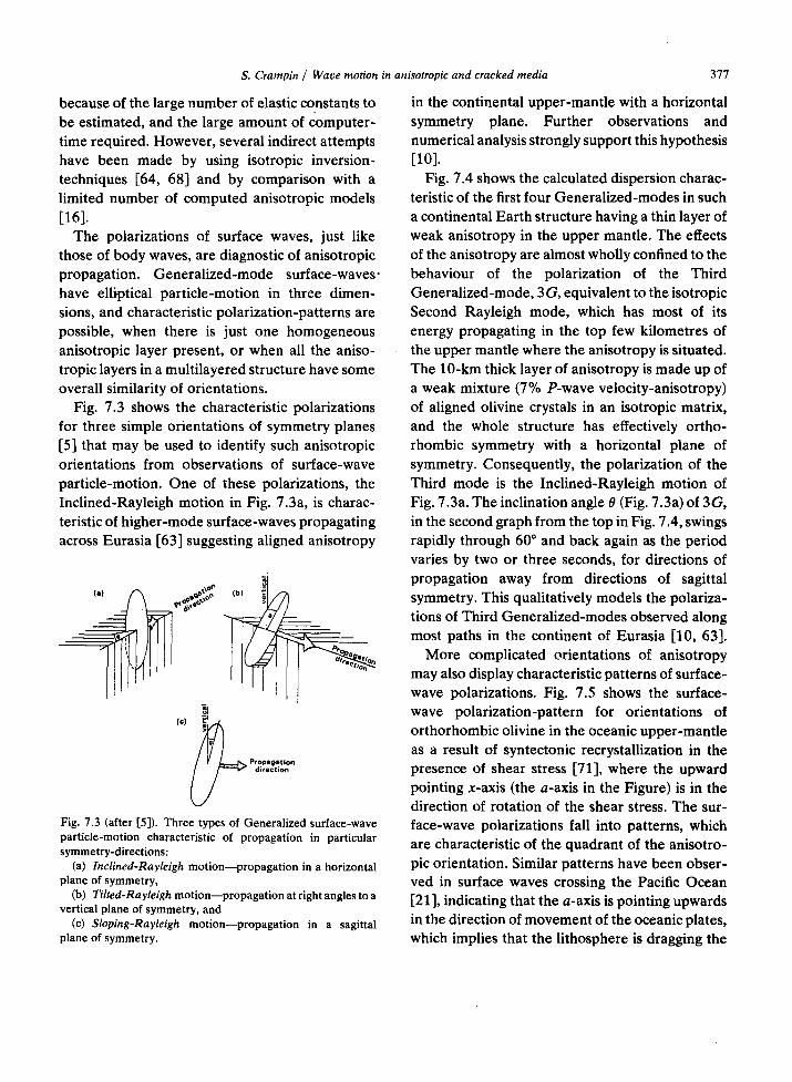
$. Crampin / Wave motion
because of the large number of elastic constants to be estimated, and the large amount of computer- time required. However, several indirect attempts have been made by using isotropic inversion- techniques [64, 68] and by comparison with a limited number of computed anisotropic models [16].
The polarizations of surface waves, just like those of body waves, are diagnostic of anisotropic propagation. Generalized-mode surface-waves. have elliptical particle-motion in three dimen- sions, and characteristic polarization-patterns are possible, when there is just one homogeneous anisotropic layer present, or when all the aniso- tropic layers in a multilayered structure have some overall similarity of orientations.
Fig. 7.3 shows the characteristic polarizations for three simple orientations of symmetry planes [5] that may be used to identify such anisotropic orientations from observations of surface-wave particle-motion. One of these polarizations, the Inclined-Rayleigh motion in Fig. 7.3a, is charac- teristic of higher-mode surface-waves propagating across Eurasia [63] suggesting aligned anisotropy
(c) "~
Propaglition direction
Fig. 7.3 (after [5]). Three types of Generalized surface-wave particle-motion characteristic of propagation in particular symmetry-directions:
(a) [nclined-Rayleigh motion--propagation in a horizontal plane of symmetry,
(b) Tilted-Rayleigh motion--propagation at right angles to a vertical plane of symmetry, and
(c) $1oping-Rayleigh motion--propagation in a sagittal plane of symmetry.
in anisotropic and cracked media 377
in the continental upper-mantle with a horizontal symmetry plane. Further observations and numerical analysis strongly support this hypothesis I;10].
Fig. 7.4 shows the calculated dispersion charac- teristic of the first four Generalized-modes in such a continental Earth structure having a thin layer of weak anisotropy in the upper mantle. The effects of the anisotropy are almost wholly confined to the behaviour of the polarization of the Third Generalized-mode, 3 G, equivalent to the isotropic Second Rayleigh mode, which has most of its energy propagating in the top few kilometres of the upper mantle where the anisotropy is situated. The 10-km thick layer of anisotropy is made up of a weak mixture (7% P-wave velocity-anisotropy) of aligned olivine crystals in an isotropic matrix, and the whole structure has effectively ortho- rhombic symmetry with a horizontal plane of symmetry. Consequently, the polarization of the Third mode is the Inclined-Rayleigh motion of Fig. 7.3a. The inclination angle 8 (Fig. 7.3a) of 3G, in the second graph from the top in Fig. 7.4, swings rapidly through 60 ° and back again as the period varies by two or three seconds, for directions of propagation away from directions of sagittal symmetry. This qualitatively models the polariza- tions of Third Generalized-modes observed along most paths in the continent of Eurasia [10, 63].
More complicated orientations of anisotropy may also display characteristic patterns of surface- wave polarizations. Fig. 7.5 shows the surface- wave polarization-pattern for orientations of orthorhombic olivine in the oceanic upper-mantle as a result of syntectonic recrystallization in the presence of shear stress [71], where the upward pointing x-axis (the a-axis in the Figure) is in the direction of rotation of the shear stress. The sur- face-wave polarizations fall into patterns, which are characteristic of the quadrant of the anisotro- pic orientation, Similar patterns have been obser- ved in surface waves crossing the Pacific Ocean [21], indicating that the a-axis is pointing upwards in the direction of movement of the oceanic plates, which implies that the lithosphere is dragging the
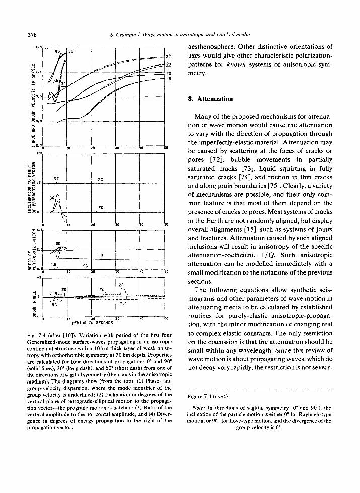
378
L. 2.E 0
101
~ a 6
S. Crampin / Wave motion in anisotropic and cracked media
aesthenosphere. Other distinctive orientations of axes would give other characteristic polarization- patterns for known systems of anisotropic sym- metry.
3G~ t
I0 20 3~ q0 S0
2G
F'G
0 I0 2~ ,50
I 3G
~ ~ F ~
¢ uJ 2G ¢: :> O.C
0 10 -5
L
II0 S0
t 0 20 PEfl lOD ,XH SECQflg$
20 20 kfJ 50
Fig. 7.4 (after [10]). Variation with period of the first four General ized-mode surface-waves propagating in an isotropic continental structure with a 10 km thick layer of weak aniso- tropy with orthorhombic symmetry at 30 km depth. Properties are calculated for four directions of propagation: 0 ° and 90 ° (solid lines), 30 ° (long dash), and 600 (short dash) from one of the directions of sagittal symmetry (the x-axis in the anisotropic medium). The diagrams show (from the top): (1) Phase- and group-velocity dispersion, where the mode identifier of the group velocity is underlined; (2) Inclination in degrees of the vertical plane of retrograde-elliptical motion to the propaga- tion vec tor - - the prograde motion is hatched; (3) Ratio of the vertical amplitude to the horizontal amplitude; and (4) Diver- gence in degrees of energy propagation to the right of the propagation vector.
8. Attenuat ion
Many of the proposed mechanisms for attenua- tion of wave motion would cause the attenuation to vary with the direction of propagation through the imperfectly-elastic material. Attenuation may be caused by scattering at the faces of cracks or pores [72], bubble movements in partially saturated cracks [73], liquid squirting in fully saturated cracks [74], and friction in thin cracks and along grain boundaries [75]. Clearly, a variety of mechanisms are possible, and their only com- mon feature is that most of them depend on the presence of cracks or pores. Most systems of cracks in the Earth are not randomly aligned, but display overall alignments [15], such as systems of joints and fractures. Attenuation caused by such aligned inclusions will result in anisotropy of the specific attenuation-coefficient, 1/Q. Such anisotropic attenuation can be modelled immediately with a small modification to the notations of the previous sections.
The following equations allow synthetic seis- mograms and other parameters of wave motion in attenuating media to be calculated by established routines for purely-elastic anisotropic-propaga- tion, with the minor modification of changing real to complex elastic-constants. The only restriction on the discussion is that the attenuation should be small within any wavelength. Since this review of wave motion is about propagating waves, which do not decay very rapidly, the restriction is not severe.
Figure 7.4 (cont.)
Note: In directions of sagittal symmetry (0 ° and 90°); the inclination of the particle motion is either 0 ° for Rayleigh-type motion, or 90 ° for Love-type motion, and the divergence of the
group velocity is 0 °.

$. Crampin / Wave motion in anisotropic and cracked media 379
-90"
/
Fig. 7.5 (after [20]). Characteristic polarizations of surface waves in (oceanic) Earth structures with olivine in the upper mantle, oriented with one vertical symmetry-plane.
This development has not been previously pub- lished, although it was presented at the Con- ference on Seismic Wave Attenuation at Stanford University in May 1979.
8 . I . B o d y - w a v e a t tenuat ion
The usual way that attenuation is introduced into isotropic wave motion [65] is by specifying the attenuation by the imaginary part of a complex velocity F = c a + i c x (the alternative of specifying complex frequencies leads to similar results). The displacement of a plane wave propagating in the x direction can then be written:
u = exp[ito (t - x / 6 ) ]
--- exp ( - a x ) exp[ito (t - x~ ca)], (8.1)
where we have expanded the complex slowness 1 / F and neglected squares of e I / ca ; a = t o / 2 Q c a ;
and the specific dissipation coefficient is [65]
1 / O = 2cI /c R. (8.2)
Attenuation may be introduced into anisotropic
wave motion by specifying imaginary parts to the elastic constants. Following the formulations of Section 2.1, we substitute plane-wave displace- ments for propagation in the xl direction:
uj = a i exp[ito ( t - x l / F) ],
for ] = 1, 2, 3, (8.3)
into the equations of motion (2.1), and obtain a similar eigenvalue problem to (2.4):
( T - OF2I)a = 0, (8.4)
where 2P is the 3 x 3 matrix with complex elements {Filkl}; and
- R • I Cjkmn = C jkmn + lC jkm n.

380
The complex 7 ~ matrix in (8.4) results in three complex-eigenvalues for the velocities of the three body-waves. For each wave we have
pt~ 2 = e R + ie I, (8.5)
where F is one of the three eigenvalues of Expanding (8.5), and neglecting squares of eI/e R, the velocity is
6 = ( e R / p ) l / 2 + i l ( e I / e R ) ( e R / p ) 1/2, (8.6)
S. Crampin / Wave motion in anisotropic and cracked media
and the dissipation coefficient corresponding to (8.2) is then
1/Q = e I / e R. (8.7)
Since most of the numerical formulations in previous sections are in complex arithmetic, almost the only alteration needed to change pro- grams for calculating wave motion in purely-elas- tic media into calculating wave motion in anelastic media is to allow the input routines to accept complex elastic-constants,
8.2. Approximate equations for the variation of a tten ua tion
The derivation of the approximate equations (6.2) for the velocity variation in planes of mirror symmetry is unaltered by taking complex rather than real elastic-constants. The coefficients in (6.2) are linear in the elastic constants. Consequently, replacing real Cikm, by complex Cikmn , the real and imaginary parts separate, and the imaginary parts satisfy a similar equation for the variation with direction as the real parts in (6.2). We have
e~ = (p 17 "2)I
=AI+B~ cos 20 +Bs I sin 20
+C~ cos 40 + C] sin 40,
I - - 2 I ese = (pVse) (8.8)
=DI +EIc cos 40 +E~ sin 40,
I ~2 )i eSR = (p SR
=F I + G~ cos 20 + G~ sin 20,
where AI, B ~ , . . . , G ~ are the same linear combinations of the imaginary elastic-constants
1 Cikm, as A, B . . . . . . Gs are of the real constants in (6.2); and E~ -CIc andE~ i = = - C , corresponding to Ec = -C¢ and E~ = -Cs in (6.2).
The dissipation coefficient for quasi P-waves can be written as
1/Op i R = e~p/ep
= (AI+B~ cos 20+B~ sin 20
+C2 cos 40 + C~ sin 40)
/ (A +Be cos 20 + B~ sin 20
+C~ cos 40 + Cs sin 40), (8,9)
with similar expressions for 1/Qs . and 1/OsR. Since B/A , C/A, E/D, and G / F are small (writing B for B~ and B . etc.), being no greater than p/100, where p is the maximum percentage of velocity anisotropy, we have as a first approximation the full equations for the dissipation coefficients:
1/Qp = (AI+B~ cos 20 +B~ sin 20
+C~ cos 40 + CI~ sin 40) /A,
1/ Qsp = ( D~ + E~ cos 40 + E l sin 4 0 ) / D, (8.10)
1/ QR = (FI + G~ cos 20 + G~ sin 20 ) / F.
In the same way that the full equations (6.2) for approximate velocity-variations contract to the reduced equations (6.3), when the angle 0 is measured from a direction of sagittal symmetry, the full equations for the dissipation coefficient (8.10) contract, under the same conditions, to the reduced equations
1/Op = (A I + B~ cos 20 + C~ cos 40) /A,
1/Ose = (DI + E~ cos 40)/D, (8.11)
1/ QsR = (FI + G~ cos 20)/F,
where the constants have the same values as in the previous equations.
These approximate equations demonstrate that the variations with direction of the dissipation coefficients have similar dependence on the angle

S. Crampin / Wave motion
of azimuth as the velocity variations. The polarities and relative amplitudes of these dissipation coefficients may of course be completely different from the velocities, and there are no a priori conditions to be imposed on the imaginary parts of the elastic constants.
These various equations are as useful for modelling attenuation as the equations (6.2) and (6.3) are for modelling velocity-variations. In media where the variation of attenuation with direction is known, either from observations, or from theoretical equations, equations (8.10) and (8.11) allow effective complex elastic-constants to be estimated. Synthetic seismograms and other characteristics of wave motion in the attenuating media can then be calculated by established pro- grams.
It is worth noting that the approximate equa- tions (8.8) and (8.11) imply that anisotropic dis- sipation coefficients 1 / Q obey the same tensor transformation for rotation as the purely-elastic constants. All the transformations are linear in the constants and the real and imaginary parts separate and transform independently.
9. Modelling two-phase materials
The presence of aligned inclusions, such as cracks, pores, or impurities, is probably the most common cause of effective anisotropy within the Earth, and possibly within many other solid materials. We shall model wave propagation through such two-phased materials by approxi- mating to the inhomogeneous material by a homogeneous solid with effective elastic-constants having the same variation of velocity (and attenu- ation) with direction as the two-phase material. Assuming the distribution of inclusions is uniform, it is always possible to make this approximation for weak concentrations of the minor phase, when the dimensions of the minor phase are small in comparison with the seismic wavelength, and it may well be quite a good approximation even for strong concentrations of large inclusions.
in anisotropic and cracked media 381
We shall be concerned here with modelling wave propagation through aligned materials whose properties vary with direction, although many of the same principles equally apply to randomly oriented distributions. The important advantages of modelling inhomogeneous material by homogeneous elastic-solids are that:
(1) Anisotropy imposes considerable con- straints on the possible variations;
(2) Anisotropy can be used to approximate to mixtures of several phases that cannot be easily modelled in any other way;
(3) Once the equivalent elastic-constants have been estimated, the properties of the wave motion, including synthetic seismograms, can be calculated by the established techniques reviewed in the previous sections.
9.1. Est imat ing effective elastic-constants [15, 19]
Any two-phased material, in so far as it has a weak concentration of the minor phase and is observed by long wavelengths, must have the same orientations of symmetry planes as one of the anisotropic symmetry-systems of Table 7.1. Examination of the material, or the forces acting on it, should indicate the orientations of these planes, and the choice of the appropriate sym- metry-system. If the symmetry planes of the material do not fit any particular system allowing for possible orientations of the principal axes, the elastic properties will be those of the system with the nearest subset of symmetry planes and the remaining planes will not be individually dis- tinguishable in the elastic behaviour. Once the appropriate symmetry-system has been identified, a f ixed number of elastic constants, suitably rotated, will specify the complete elastic-proper- ties of the two-phase material. Thus modelling a three-dimensional velocity-distribution, with unknown limitations on the variations, can be reduced to solving for a finite number of elastic constants in a known symmetry system.
These constants can be found by equating the approximate equations (6.2) or (6.3) to the

382 S. Crampin / Wave motion
velocities in a few directions in symmetry planes. It can usually be arranged that the angle is measured from a direction of sagittal symmetry. The reduced equations (6.3) then apply, and are completely specified, and up to seven elastic constants deter- mined, by the velocities at 0 °, 45 °, and 90 ° for qP; 0 ° and 45 ° for qSP; and 0 ° and 90 ° for qSR, This process is repeated for other symmetry planes until all the required constants are specified. There is usually a great deal of redundancy, and in some systems of symmetry all the constants are deter- mined from a very few specified directions. In a material with cubic symmetry, for example, the three elastic constants are determined by the velocities in directions 0 ° and 45 ° for qP, and 0 ° for the quasi shear-waves in any of the symmetry planes.
Equations (6.2) and (6.3) are quite good approximations even for strong anisotropy [22]. However, the exact velocity-variations for a set of elastic constants, determined by the eigenvalue technique of Section 2, for example, may be a little different from those of the approximate equations. A few empirical adjustments in the procedure for determining the elastic constants, in order to balance the 40 contributions to the qP and qSP variations, may improve the fit of the elastic constants to the velocity variations of the two- phase material.
In modelling the combination of several dis- tributions of inclusions in an isotropic matrix (such as an intersecting system of cracks), we make the assumption that, to a first approximation, the effects may be obtained by directly combining the effects of the separate distributions in specified directions. In such corresponding directions, shear waves have the same polarizations in each separate distribution, and their properties may be combined, so that the proportional reduction (or increase) in the velocity of the isotropic matrix caused by each distribution separately may be multiplied together to give the reduction (or increase) in velocity of the combined system. Elastic constants are determined in the same way as in simple two-phase media. If sufficient cor-
in anisotropic and cracked media
responding directions can be found, the fixed number of constants for the appropriate sym- metry-system can be determined, and the aniso- tropic tensor necessarily specifies the velocity variations in all other directions. These techniques have allowed velocity variations to be determined for biplanar and triplanar crack-systems [15], cracks with co-planar normals [25], and mixtures of interleaved dry and saturated cracks [19]. Such intersecting systems of cracks are very common, and this technique of determining constants from a few corresponding directions and allowing the anisotropic tensor to specify the velocities in the remaining directions is a very effective way of modelling complicated two-phase systems.
9.2. Propagation in cracked solids [15]
Crampin [15] applied these techniques for modelling two-phase materials to cracked iso- tropic-solids. Elastic constants were derived for homogeneous purely-elastic solids possessing the same velocity variations as the theoretical expres- sions of Garbin and Knopoff [76, 77, 78] for waves scattered by propagation through an isotropic media with weak concentrations of small, thin, parallel penny-shaped cracks. Garbin and Knopoff gave expressions for the velocity variations in terms of angle of incidence to the cracks and the polarization of the wave, and made neither direct nor indirect assumptions of anisotropy. Note that the techniques presented here are not dependent on these particular determinations of Garbin and Knopoff. Any valid velocity-variations can be treated in the same way.
The solid lines in Fig. 4.2 show the theoretical velocity-variations for dry and saturated dis- tributions of thin parallel cracks. The largest crack
2 density of e = 0.1 is equivalent to, say, one 1 cm crack in every 1 cm 3 (crack densities in competent rock can certainly exceed this crack density). Such crack distributions of parallel cracks possess hexagonal symmetry (transversely-isotropic symmetry, if the axis is vertical), and are described by five elastic-constants (see Fig. 7.1).

S. Crampin / Wave motion
Consequently, the constants can be determined by equating the reduced equations of five velocities in directions: 0 °, 45 °, and 90 ° for qP; 0 ° for qSP or qSR ; and 90 ° for qSR, where the angles are angle of incidence to the cracks measured from the symmetry-axis normal to the crack faces. The exact velocity variations of the derived aniso- tropic-tensors are indicated by the dashed lines in Fig. 4.2.
The agreement between the solid and dashed lines is good, although some empirical adjustment to the constants improved the fit for dry cracks. It is worth noting the agreement, despite being derived by completely different techniques, between the velocity variations through parallel cracks of Garbin and Knopoff, and the approximate equa- tions (6.2) and (6.3) for the anisotropic velocity- variations. Both variations have approximately equal but opposite sign 40 contributions to the squares of qP and qSP velocity variations.
Velocity variations have also been derived [15] for propagation through various intersecting systems of parallel cracks with the techniques of the previous Section. As examples: Fig. 9. la shows the theoretical and purely-elastic variations, in the plane perpendicular to the intersection, of a biplanar system of dry cracks with equal crack- densities intersecting at 90 °, and Fig. 9.1b shows the variations, in a plane parallel to one of the crack systems, of a triplanar system of saturated cracks with equal crack-densities intersecting in an orthogonal corner. These examples show crack systems with equal crack-densities intersecting at 90 °, but all variations of biplanar systems can be modelled [19], as can all combinations of triplanar systems, for which one of the systems is perpendi- cular to the intersection of the other two systems. Many naturally occurring systems of cracks have various biplanar and triplanar distributions.
There are very few observations of velocity variations in any sort of crack system to compare with these theoretically derived determinations: Nur and Simmons [79] subjected Barre granite, which possessed a nearly random crack-system, to uniaxial stress. They attributed the velocity varia-
in anisotropic and cracked media
a b 6 .~ 6.C
5 . 5 S.E
383
5 . 0 5 . [
t i .~ q . 0
g
3.5 7 - 3 . 5
°Z \ 3.8 ~ ~P"-~ QSR ~3.C
- I 2 . 5 03 2...
8 38 68 9~ 8 30 68
QSP QSR
S0
Fig. 9.1 (after [15]). (a) Velocity variations over the plane normal to the axis of intersection of an orthogonal biplanar- system of two sets of dry parallel-cracks with the same crack- density of 0.08 in the isotropic solid of Fig. 4.1. Angles of incidence are measured from one of the crack faces.
(b) Velocity variations over the plane parallel to one of the cracks of an orthogonal tr iplanar-system of three sets of saturated parallel-cracks with the same crack-density of 0.07 in the isotropic solid of Fig. 4.1. Angles of incidence are measured from one of the crack faces.
The notat ion is the same as in Fig. 4.2.
tions they observed to differential closure of cracks normal to the direction of stress, producing a system of cracks with co-planar normals. Very similar velocity-variations can be obtained by integrating the theoretical variations for parallel cracks about an axis in one of the planes to produce a co-planar normal crack distribution [25].
Bamford and Nunn [80] observed P-wave velo- city anisotropy in 70-m diameter experiments over Carboniferous Limestone with a pronounced system of vertical cracks. They found variations

384
differing by over 0.5 km/sec at three sites within 3 km of each other, despite crack alignments being consistent over a very large region. These obser- vations were inverted [19] to yield crack dis- tributions with similar densities and alignments at the three sites. The differences in the velocity variations were attr ibuted to different percentages of water saturation in interleaved dry and
saturated cracks. Such interleafing may occur above the watertable, whenever there is a large variation in the size of the cracks in an otherwise impermeable solid. Wide cracks will be dry, whereas fine cracks may retain water f o r long periods of t ime by surface tension and capillary
action.
9.3. Propagation in at tenuat ing solids
S. Crampin / Wave motion in anisotropic and cracked media
a 8 , 5
8.ff
7.5
6.5
zS.
>-
HS.
o
d Ld > CE
>-- C~
~3 ff 3(] 6(]
flip
b ff . ff l ff
O. 008
CI. ~06
O. OOtl
q
z ft. 002
OSB o:
z OSP w
gO
1,, 0 35 68 9~
OSP
Many of the techniques discussed in the pre- vious two sections also apply, with minor modifications, to modelling at tenuation in two- phase materials with the equations of Section 8.
Chat ter jee, Mal, Knopoff and Hudson [72] determined theoretical expressions for the varia- tion of both velocity and at tenuation of waves propagat ing through parallel cracks filled with a viscous fluid, and included both the effects of scattering at the crack faces, by a technique similar to that used previously in [76, 77, 78], and the effects of the viscous at tenuation within the cracks. The variations are expressed in terms of the angle of incidence to the cracks and the polarization of each wave. We illustrate the techniques of model- ling by showing the variations with direction of velocity and at tenuation in QST001, and calculat- ing synthetic seismograms. QST001 is a structure of parallel viscous-filled cracks (parameters in caption to Fig. 9.2) very approximately modelling lenses of melt in the Ear th ' s low-velocity-channel.
Fig. 9.2 shows the variation with direction of the velocity and at tenuation of a 1 Hz wave in QST001. The values of velocity and attenuation are, in some sense, reciprocals of each other: the at tenuation of each wave type is greatest in direc- tions where the velocity is least and vice versa. The
Fig. 9.2. Variations with angle from the vertical of (a) phase velocities, and (b) attenuation coefficients, I/Q, of 1 Hz body- waves propagating through QST001, which is a structure, with hexagonal symmetry, of circular parallel viscous-filled cracks with density, radius, aspect-ratio, and coefficients of viscosity of 0.1, 100 m, 0.1 and 5 x l0 s poise, respectively, in an isotropic solid: p = 3.4 gm/cm 3, a = 7.6 km/sec, and ~ = 4.2 km/sec. Solid lines are from the theoretical expressions of [72], and dashed lines are exact values from the complex elastic-tensor derived by fitting the approximate equations (6.3) and (8.11) to
the theoretical values.
form of the velocity variations is similar to those in
the saturated cracks in Fig. 4.2c (the derivations of the formulae are similar), although the average velocities are very different due to the different velocities in the uncracked solids.
Fig. 9.3 shows synthetic seismograms of 1 Hz shear-wave pulses propagat ing at normal incidence through a 100 km thick slab of QST001 for a range of crack orientations. The initial shear pulses have polarizations intermediate between the Z and T axes. Fig. 9.3 shows a marked varia- tion of pulse amplitude with the crack orientation, and can be contrasted with the seismograms in Fig. 4.3a, for propagat ion through a non-at tenuat ing structure, which have a very similar pat tern of arrivals, but with equal-ampli tude pulses.

s. Crampin / Wave motion in anisotropic and cracked media
Note that the attenuated seismograms in Fig. 9.3 are calculated for 1 /Q corresponding to the 1 H z values in Fig. 9.2, and the frequency dependence of the expressions of [72] has not been taken into account in the calculation. The incident pulse,
u(t) = t 2 exp - ( to t /k) 2 sin tot,
where t is time, and k (=3) controls the damping, has a dominant 1 Hz component, and smaller- amplitude higher-frequency components associ- ated with the transient nature of the pulse [12]. The higher-frequency components are evident in the broadening of the pulse in the more attenuated signals (particularly noticeable in the top and bottom records of Fig. 9.3). This is because the specific attenuation coefficient 1 /Q represents a proportional decrease in amplitude per wavelength. The higher frequencies have more wavelengths, and correspondingly greater
z B T
R
T
Z
R
T
Z
R
T
Z
R
Z ~
-I SEC
1 HZ Su,5 THRO' IOOKH QSTOOt fiT 50RIENTNS
Fig. 9.3. Synthetic seismograms of 1 Hz shear-waves with intermediate polarizations propagating at normal incidence through a 100 km thick slab (Fig. 4.1) with five orientations of QST001, with the initial (top) orientation with the symmetry axis in the Radial direction, and then successively rotated by
22.5 ° about the Z axis.
385
attenuation over any given length of path, and the transient arrival is smoothed.
This phenomenon of pulse broadening may occur for any wave and path direction for which to/Qc (8.1) is frequency dependent. In the formu- lation of Chatterjee et aL [72], to/Qc is independent of frequency only for purely viscous damping. We conclude that the absence of pulse broadening in attenuated waves through cracked media may be diagnostic of viscous attenuation.
10, Shear-wave polarizat ion-anomalies [8, 13,
15, 24, 26]
The existence of shear-wave polarization- anomalies can be inferred from theory, but it is difficult to realize the subtle yet characteristic effect these anomalies have on the particle motion of the shear wavetrain without numerical or observational experiments.
The behaviour of shear waves crossing an anisotropic region is illustrated schematically in Fig. 10.1. The shear wave necessarily has to split, on entry into the anisotropic region, into two phases with polarizations orthogonal with respect to the propagation direction and fixed for the particular direction through the anisotropy. This splitting phenomenon is also called shear-wave birefringence, and shear-wave double-refraction.
ISOTROPIC REGION
/
Fig. 10.1. Schematic representation of shear-wave splitting.

386 S. Crampin / Wave motion
In general, the two shear-waves with distinct polarizations will travel at different velocities and arrive at the exit interface at different times. The delay is proportional to the degree of differential shear-wave anisotropy in that particular direction, and to the length of the path through the aniso- tropic region. The delay between the shear arrivals results in a polarization anomaly in the shear wavetrain, which will be preserved unchanged for any following isotropic propagation, since the velocity of shear waves in isotropic solids is independent of the polarization. Since it is difficult to devise isotropic structures that can split shear body-waves, the recognition of split arrivals in a shear wavetrain is a strong indication of anisotropy somewhere along the path, particularly if the splitting is not into SH and SV waves.
Note that the delay between the two split shear- waves is a rather more direct measurement of physical parameters than is the case with many seismic observations. The delay between the two phases is measured directly from the seismogram, and is directly proportional to the two things of particular interest to us here: the length of the path through the anisotropie region; and the relative difference in the slownesses of the two split shear- waves for that particular direction of propagation.
This suggests techniques for estimating both the degree of anisotropy and its symmetry structure, if there are enough observations of the shear-waves propagating in a variety of directions through the anisotropic medium. There are two quantities easily determined from any seismogram displaying shear-wave splitting: the time delay between the two shear arrivals; and the polarization of the first (faster) shear-wave. The later arriving shear-wave is usually superimposed on the first arrival, and although its arrival time may be picked from polarization diagrams, its polarization will be more difficult to determine reliably.
Fig. 10.2 displays shear-wave delays and polarizations in stereograms for shear-wave delays and polarizations for propagation in a 10-km sphere of orthopyroxene projected on to the z-cut and two more generally oriented cuts. The delays
in anisotropic and cracked media
and polarizations are calculated for the group- velocity arrivals, by the techniques of Crampin and McGonigle [24], since it is the group velocity which is observed in all cases. It is easy to plot observations of shear-wave delays and polariza- tions in such stereograms, whether they are observations of rays surrounding a point source, or of teleseisms propagating through a layer of anisotropy in the upper mantle. Generally orien- ted anisotropy (or generally oriented planes of projection) may lead to complicated asymmetrical patterns in the stereograms, such as those in Fig. 10.2c. However, once observations of delays and polarizations in one plane of projection have been tabulated in machine-readable form, they can easily be rotated into stereograms for other planes of projection in order to search for symmetry planes and other identifiable properties of the anisotropy. It is suggested that such stereograrns are a powerful technique for estimating anisotropy from observations.
11. Discussion, application, and speculation
Many of the properties of wave motion in anisotropic media have been known for many years, although it is only since the numerical modelling-programs, outlined in this review, have been developed that the effects of these proper- ties can be properly evaluated. One of the major results of this development is the recognition that quasi shear-wave polarization-anomalies are a powerful technique for both diagnosing the presence of anisotropy and for estimating some of its parameters. The technique involves analysing the particle motion in shear-wavetrains. Particle motion has been neglected in conventional seis- mology, and part of the reason may well be that unsuspected anisotropy has frequently introduced previously-uninterpretable complications. It is hoped that one of the effects of these aniso- tropic developments will be to reopen interest in studies of, particularly shear-wave, particle- motion.

a
20
S. Crampin / Wave motion in anisotropic and cracked media
N N ./-
.1" ,1" -I" -I" • \" ,/" .~" -/" 4"
÷ -1- -1- -I- "I, 1, 1. "1- "1-
1, "1- 1. I- 1. 1- ~I'-
1. % o
I
+ 1- 1-
i -V + -V q -
+ -\" .I" .I" ,t" ,\" ,__ -I- .I" .I" ,I"
: I : :I: + .1" + . / -
11
2o
N i d. /" "v- % %
¢ ,l" -1" -I" + "l- t- 1. \ /,P -I" -l" -I" + "I- I- I- I,',, I -1- -1- -I- + - I - -V -I- t ;4, "/, t . -I- 4- - - -1- -I- .I- ,\" ,'4
• ,, -/. -/. -I- - - .V .V X / , , 7 . > - : - ~ . \ . , .
, , , x - i - .'.< / ,
387
C
2o
N
o
N
I , - " .-,< .\. -\" % % % \
I / × -\" -V -\" % "\- % "\- ~, I. \ -I- -I- -I- -I- -]- -I- "I. ~, \ ~'I,'[- -\- ~, -I--I-.I'./"
\ ' , . >: "I" ~ - - ./" d" I
Fig. 10.2. Stereographic projections of the relative shear-wave delays (in hundredths of a second) and polarizations (projected on to the horizontal plane) for propagation through a 10 km focal sphere of orthopyroxene. On the left of each delay s tereogram is a north-south section. The solid bar of the polarizations is the projection of the faster (first arrival) quasi shear-wave, qS1, and the broken bar is the polarization of the slower shear-wave, qS2. The small solid circles on the delay stereograms mark the zero positions of point singularities on the equivalent phase-velocity stereograms. The orientations are:
(a) z-cut horizontal, with x axis pointing north; (b) as in (a), but rotated 40 ° about the y axis; and (c) as in (b), but rotated 20 ° about the x axis. Note: there are irregularities in the contours of delays near some of the singularities due to the grid points of the systems routines
being too coarse.

388 S. Crampin / Wave motion in anisotropic and cracked media
The anisotropic developments reviewed here cover a wide field, and demonstrate that the solu- tion of almost any problem in anisotropic pro- pagation can at least be formulated, and very often solved (at the cost of considerable numerical analysis), if the solution exists for isotropic pro- pagation. This opens the possibility of using seis- mic waves to examine the internal structure of the medium through which they propagate. It is suggested that the presence of anisotropy should not be though of as an unnecessary and complicat- ing nuisance, but should be valued as a means of investigating the internal constitution of the medium [9], its present or previous stress-dis- tribution [14, 81], and, perhaps most important, the presence, orientation, and distribution of aligned cracks [15, 19, 26].
The other major result of the developments reviewed here is that modelling propagation through material with aligned cracks by propaga- tion through homogeneous anisotropic solids, in effect, opens up a whole new class of material to wave-propagation calculations. Since cracks in solids are a very common, if not ubiquitous phenomenon, which are usually aligned by stress at some stage in their growth, this development may have very wide applications. Modelling cracks by determining the effective real elastic-constants, when the dimensions of the cracks are sufficiently small compared with the seismic wavelength, allows the velocity and amplitude variations of both P and shear-waves to be calculated, as well as the delays and polarizations of the split shear- waves. If the dimensions of the cracks are sufficiently large for attenuation to be important, the velocity variations are probably not seriously disturbed [19], and the attenuation can be modelled, by the equations for anisotropic anelas- tic wave-motion using complex elastic-constants. All the analytical results, computing techniques, and computer programs for purely-elastic aniso- tropic wave-motion, apply equally well to attenu- ating media, with the one modification: that the elastic constants are changed from real to complex quantities.
The developments reviewed here may be applied wherever anisotropy or aligned cracks exist in any solid structure. A number of possible applications have been identified:
(1) Velocity anisotropy has been widely identified in the oceanic, and some continental, upper mantle, and is probably due to preferred crystal orientations. There are reasons to believe that this anisotropy may be more extensive in the upper mantle than is usually observed [14, 81]. In that case, every wave that penetrates the upper mantle may require anisotropy to be considered in the interpretation, if the observations have sufficient resolution.
Most applications, however, are likely to be associated with the effective anisotropy caused by the presence of aligned cracks, which is probably a very common phenomenon.
(2) Extensive dilatancy-anisotropy appears to be associated with active seismic-regions [26, 82]. If this hypothesis can be confirmed, it seems that investigations of shear-wave polarization anomal- ies may be one of the most promising techniques for monitoring changes of stress before ear- thquakes that has yet been suggested. There are possible applications to earthquake prediction [26], and monitoring induced seismicity associated with reservoir loading, and with rock bursts and acoustic emission in mines.
(3) Hot-dry-rock geothermal-heat extraction sets up aligned cracks deep in hot competent-rock. The actual geometry of the cracks is important for understanding the processes involved, as well as for the continued exploitation of each reservoir. Since the interpretation of seismograms from down-weU three-component geophones is one of the principal techniques for mapping the crack geometry, modelling synthetic seismograms by suitable anisotropic structures may well be important for interpreting the crack geometry correctly.
(4) Many oil and water resources are in rock with aligned cracks or pores. Investigations of shear waves propagating through such structures may give estimates of the degree of cracking, the

$. Crampin / Wave motion
alignment of the cracks, and the proportion of liquid-filled cracks [19]. In addition, many oil reservoirs lie beneath great thicknesses of oil shale, which may be anisotropic [83], and, unless the anisotropy is correctly modelled, the structures below the shales will be difficult to interpret cor- rectly.
(5) Non-destructive testing for stress is increas- ingly important for monitoring many engineering projects. A major technique for investigating the stress is examining the effects of the stress-induced anisotropy on seismic microwaves. At pesent, the techniques usually involve P-waves, but this review demonstrates that the delays and polariza- tions in shear-wavetrains contain much additional and easily accessible information.
The above applications, although largely unconfirmed, have considerable promise, as some degree of effective anisotropy certainly exists in a great many structures and there are now tech- niques by which it can be examined. Many other, more speculative applications could also be suggested.
This is a review of work currently in progress, some new results have been obtained while the review was being written, and incorporated where possible. Clearly, the presence of anisotropy in wave-motion studies is no longer the complicating nuisance it has been in the past. Anisotropic wave- motion is comparatively well understood. Its properties can be calculated. There are now ways to estimate its properties from observations, and it has the potential for answering many detailed questions about the interior structure of solids.
Acknowledgements
I am very grateful to Markus Bath, who showed me peculiarities in the wavetrain of higher modes propagating to Uppsala from a Ryukyu Islands earthquake, which first awakened my interest in anisotropic wave-propagation.
in anisotropic and cracked media 389
The work reviewed here is the outcome of collaboration with many people, too numerous to mention individually. They are the authors or coauthors of the first 31 items of the reference list, and have each contributed significantly to this development. I particularly thank David B. Taylor of the Edinburgh Regional Computing Centre, who has contributed in innumerable ways over many years through discussion, programming, analytical advice, and in commenting on this manuscript--without him this development would not have been possible. I am grateful to Robert McGonigle for his comments on the manuscript and for providing much assistance in computing. I also thank Tolya Levshin of the Institute of Physics of the Earth, Moscow, for suggesting I write this review, and for commenting on the manuscript, much of which was written at the Institute of Physics of the Earth, while on an exchange visit arranged by the Royal Society and the Academy of Sciences of the USSR. This work is supported by the Natural Environment Research Council and is published with the approval of the Director of the Institute of Geological Sciences (N.E.R.C.).
References
[1] S. Crampin, "The dispersion of surface waves in multi- layered anisotropic media", Geophys. J.R. Astr. Soc. 21, 387-402 (1970).
[2] S. Crampin and D.B. Taylor, "The propagation of surface waves in anisotropic media", Geophys. J.R. Astr. Soc. 25, 71-87 (1971).
[3] G.A. Armstrong and S. Crampin, "Piezoelectric surface- wave calculations in multilayered anisotropic media", Electron. Lett. 8, 521-522 (1972).
[4] G.A. Armstrong and S. Crampin, "Preferential excitation of 2nd-mode piezoelectric surface waves in zinc-oxide- layered substrates", Electron. Lett. 9, 322-323 (1973).
[5] S. Crampin, "Distinctive particle motion of surface waves as a diagnostic of anisotropic layering", Geophys. J.R. Astr. $oc. 40, 177-186 (1975).
[6] S. Crampin, "A comment on 'The early structural evolu- tion and anisotropy of the oceanic upper mantle' ", Geo- phys. J,R. Astr. Soc. 46, 193-197 (1976).
[7] D. Bamford and S. Crampin, "Seismic anisotropy--the state of the art", Geophys. J.R. Astr. Soc. 49, 1-8 (1977).
[8] S. Crampin, "A review of the effects of anisotropic layer- ing on the propagation of seismic waves", Geophys. J.R. Astr. Soc. 49, 9-27 (1977).

390 S. Crampin / Wave motion in anisotropic and cracked media
[9] S. Crampin and D. Bamford, "Inversion of P-wave velo- city anisotropy", Geophys. J.R. Astr. $oc. 49, 123-132 (1977).
[10] S. Crampin and D.W. King, "Evidence for anisotropy in the upper mantle beneath Eurasia from generalized higher mode seismic surface waves", Geophys. J.R. Astr. Soc. 49, 59-85 (1977).
[11] C.M. Keith and S. Crampin, "Seismic body waves in anisotropic media: reflection and refraction at a plane interface", Geophys. J.R. Astr. Soc. 49, 181-208 (1977).
[12] C.M. Keith and S. Crampin, "Seismic body waves in anisotropic media: propagation through a layer", Geo- phys. J.R. Astr. Soc. 49, 209-223 (1977).
[13] C.M. Keith and S. Crampin, "Seismic body waves in anisotropic media: synthetic seismograms", Geophys. J.R. Astr. Soc. 49, 225-243 (1977).
[14] S. Crampin, "Palaeoanisotrpy in the upper mantle", Nature 270, 162-163 (1977).
[15] S. Crampin, "Seismic-wave propagation through a cracked solid: polarization as a possible dilatancy diag- nostic", Geophys. J.R. Astr. Soc. 53, 467-496 (1978).
[16] S.C. Kirkwood, "The significance of isotropic inversion of anisotropic surface-wave dispersion", Geophys. J.R. Astr. $oc. 55, 131-142 (1978).
[17] D.B. Taylor and S. Crampin, "Seismic surface waves in anisotropic media: propagation in a homogeneous piezo- electric halfspace", Proc. R. Soc. A. 364, 161-179 (1978).
[18] D.B. Taylor, "On the existence of elastic surface waves", Quart. J. Mech. Appl. Math. 31, 335-347 (1978).
[19] S. Crampin, R. McGonigle and D. Bamford, "Estimating crack parameters from observations of P-wave velocity anisotropy", Geophys. 45, 345-360 (1980).
[20] S.C. Kirkwood and S. Crampin, "Surface-wave propaga- tion in an ocean basin with an anisotropic upper-mantle: numerical modelling", Geophys. J.R. Astr. Soc. 64, 463- 485 (1981).
[21] S.C. Kirkwood and S. Crampin, "Surface-wave propaga- tion in an ocean basin with an anisotropic upper-mantle: observations of polarization anomalies", Geophys. J.R. Astr. Soc. 64, 487-497 (1981).
[22] S. Crampin and S.C. Kirkwood, "Velocity variations in systems of anisotropic symmetry", J. Geophys. 49, 35-42 (1981).
[23] S. Crampin and M. Yedlin, "Shear-wave singularities of wave propagation in anisotropic media", J. Geophys. 49, 43-46 (1981).
[24] S. Crampin and R. McGonigle, "The variation of delays in stress-induced anisotropic polarization-anomalies", Geophys. J.R. Astr. $oc. 64, 115-131 (1981).
[25] S. Crampinand B.J. Radovich, "Inversion of CDPgathers for a single anisotropic layer", Geophys., submitted (1981).
[26] S. Crampin, R. Evans, B. O~er, M. Doyle, J.P. Davis, G.V. Yegorkina and A. Miller, "Observations of dila- tancy-induced polarization anomalies and earthquake prediction", Nature 296, 874-877 (1980).
[27] D.C. Booth and S. Crampin, "Calculating synthetic seis- mograms in anisotropic media by the reflectivity tech-
nique: theory", Inst. Geol. Sci., GSU Report No. 133 (1980).
[28] S. Crampin, R. Evans, M. Doyle and J.P. Davis, "Com- ments on papers about shear-wave splitting in dilatancy- induced anisotropy by I.N. Gupta and by A. Ryall and W.U. Savage", Bull. Seism. Soc. Amer. 71, 375-377 (1981).
[29] S. Crampin, R.A. Stephen and R. McGonigle, "The polarizations of P-waves in anisotropic media", Geophys. J.R. Astr. Soc., submitted (1981).
[30] M. Doyle, R. McGonigle and 8. Crampin, "The effects of crack anisotropy on the hypocentral locations of local earthquakes", Geophys. J.R. Astr. Soc., submitted (1981).
[31] S. Crampin, "A note on 'Possible forms of anisotropy of the uppermost mantle under coeans' by George E. Backus", J. Geophys. Res., submitted (1981).
[32] D.L. Anderson, "Elastic wave propagation in layered anisotropic media", J. Geophys. Res. 66, 2953-2963 (1961).
[33] D.G. Harkrider and D.L. Anderson, "Computation of surface wave dispersion for multilayered anisotropic media", Bull. Seism. Soc. Amer. 52, 321-332 (1962).
[34] D.L. Anderson, "Love wave dispersion in heterogeneous anisotropic media", Geophys. 27, 445-454 (1962).
[35] V.S. Budayev, "The distribution of vibrations from a concentrated impulse source in an anisotropic medium", (in Russian) Prikl. Mech, 9, 67-73 (1973).
[36] V.S. Budayev, "Propagation of vibrations from a point source in an elastic anisotropic halfspace", (in Russian) lzv. Akad. Nauk. SSSR, Fiz. Zemli 2, 38-47; 102-107 of AGU English edition (1977).
[37] V.S. Budayev, "A point source of disturbance in an elastic anisotropic medium", (in Russian) Izv. Akad. Nauk. SSSR, Fiz. Zemli 1, 44-53; 28-33 of AGU English edition (1978).
[38] M.J.P. Musgrave, Crystal Acoustics, Holden-Day, San Francisco (1970).
[39] A.E.H. Love, "A Treatise on the Mathematical Theory of Elasticity", 4th edn, Dover, New York (1944).
[40] M.J. Lighthill, "On magneto-hydrodynamic waves and other anisotropic wave motion", Phil. Trans. R. Soc. A. 252, 397-430 (1960).
[41] M. Kumazawa, "The elastic constants of single-crystal orthopyroxene", J. Geophy. Res. 74, 5973-5980 (1969).
[42] G.F.D. Duff, "The Cauchy problem for elastic waves in an anisotropic medium", Phil. Trans. R. Soc. A. 252, 249- 273 (1960).
[43] J. L. Synge, "Elastic waves in anisotropic media", J. Math. Phys. 35, 323-334 (1957).
[44] G.W. Postma, "Wave propagation in a stratified medium", Geophys. 20, 780-806 (1955).
[45] G.F. Miller and M.J.P. Musgrave, "On propagation of elastic waves in aeolotropic media. III. Media of cubic symmetry", Proc. R. Soc. A. 236, 352-383 (1956).
[46] R. Burridge, "The singularity on the plane lids of the wave surface of elastic media with cubic symmetry", Q.J. Mech. AppL Maths. 20, 41-56 (1967).

S. Crampin / Wave motion in anisotropic and cracked media 391
[47] A.N. Stroh, "Steady state problems in anisotropic elasti- city", J. Math. Phys. 41, 77-103 (1962).
[48] F. Gilbert and G.E. Backus, "Propagator matrices in elastic wave and vibration problems", Geophys. 31, 326- 332 (1966).
[49] P. Chadwick and G.D. Smith, "Foundations of the theory of surface waves in anisotropic elastic materials", Advances in Appl. Mech. 17, 303-382 (1977).
[50] G.W. Farnell, "SAW propagation in piezoelectric solids", Wave Electron. 1-24 (1976).
[51] H.F. Tiersten, "Wave propagation in an infinite piezo- electric plate", 3". Acoust. $oc. Amer. 35, 234-239 (1963).
[52] J.F. Nye, Physical Properties of Crystals, Oxford Uni- versity Press, Oxford (1957).
[53] K. Fuchs, "The reflection of spherical waves from tran- sition zones with arbitrary depth-dependent elastic moduli and density", J. Phys. Earth 16, 27-41 (1968).
[54] K. Fuchs and G. Miiller, "Computation of synthetic seismograms with the reflectivity method and comparison with observations", Geophys. ZR. Astr. Soc. 23, 417-433 (1971).
[55] V.M. Babich and A.S. Alekseev, "A ray method of computing wave front intensities", (in Russian) Izv. Akad. Nauk, $$SR, Geofiz. 1, 17-31; 9-15 of AGU English edition (1958).
[56] V. (~erven~,, I.A. Molotkov and I. Pgen~fk, "Ray method in seismology", Univ. Karlova, Praha (1977).
[57] J.L. Synge, "Flux of energy for elastic waves in anisotropic media", Proc. R. Irish Acad. A. 58, 13-21 (1956).
[58] D. Bamford, "Pn velocity anisotropy in a continental upper mantle", Geophys. J.R. Astr. Soc. 49, 29-48 (1977).
[59] D. Bamford, M. Jentsch and C. Prodehl, "Pn anisotropy studies in northern Britain and the eastern and western United States", Geophys. ZR. Astr. $oc. 57, 397-429 (1979).
[60] R. Kind, "Computation of reflection coefficients for layered media", J. Geophys. 42, 191-200 (1976).
[61] B.L.N. Kennett, "Reflections, rays, and reverberations", Bull. Seism. Soc. Amer. 64, 1685-1696 (1974).
[62] V. Pereyra, W.H.K. Lee and H.B. Keller, "Solving two- point seismic-ray tracing problems in a heterogeneous medium, Part 1. A general adaptive finite difference method", Bull. Seism. $oc. Amer. 70, 79-100 (1980).
[63] S. Crampin, "Higher modes of seismic surface waves: propagation in Eurasia", Bull. Seism. Soc. Amer. 56, 1227-1239 (1966).
[64] D.W. Forsyth, "The early structural evolution and aniso- tropy of the oceanic upper mantle", Geophys. J.R. Astr. Soc. 43, 103-162 (1975).
[65] F. Schwab and L. Knopoff, "Fast surface wave and free mode computations", Meth. Computat. Phys. 11, 87-180 (1972).
[66] Iq.A. Haskell, "The dispersion of surface waves in multi- layered media", Bull. Seism. $oc. Amer. 43, 17-34 (1953).
[67] J.W. Schlue and L. Knopoff, "Shear wave polarization anisotropy in the Pacific Basin", Geophys. J.R. Astr. Soc. 49, 145-165 (1977).
[68] M. Cara, A. Nercessian and G. Nolet, "New inferences from higher mode data in western Europe and northern Eurasia", Geophys. J.R. Astr. Soc. 61,459-478 (1980):
[69] G.E. Backus, "Possible forms of seismic anisotropy of the uppermost mantle under oceans", Y. Geophys. Res. 70, 3429-3439 (1965).
[70] M.L. Smith and F.A. Dahlen, "The azimuthal depen- dence of Love and Rayleigh wave propagation in a slightly anisotropic medium", J. Geophys. Res. 78, 3321-3333 (1973).
[71] H.G. Av~ Lallemant and N.L: Carter, "Syntectonic recrystallization of olivine and modes of flow in the upper mantle", Geol. Soc. Amer. Bull. 81, 2203-2220 (1970).
[72] A.K. Chatterjee, A.K. Mal, L. Knopoff and J.A. Hudson, "Attenuation of elastic waves in a cracked, fluid-saturated solid", Math. Proc. Camb. Phil. Soc. 88, 547-561 (1980).
[73] G.M. Mavko and A. Nur, "Wave attenuation in partially saturated rocks", Geophys. 44, 161-178 (1979).
[74] R. O'Connell and B. Budiansky, "Viscoelastic properties of fluid-saturated crack solids", J. Geophys. Res. 82, 5719-5735 (1977).
[75] D.H. Johnston, M. N. Toks6z and A. Timur, "Attenua- tion of seismic waves in dry and saturated rocks: II. Mechanisms", Geophys. 44, 491-511 (1979).
[76] H.D. Garbin and L. Knopoff, "The compression modulus of a material permeated by a random distribution of free circular cracks", O. Appl. Math. 30, 453-464 (1973).
[77] H.D. Garbin and L. Knopoff, "The shear modulus of a material permeated by a random distribution of free circular cracks", O. Appl. Math. 33, 296-300 (1975).
[78] H.D. Garbin and L. Knopoff, "Elastic moduli of a medium with liquid-filled cracks", O. Appl. Math. 33, 301-303 (1975).
[79] A. Nut and G. Simmons, "Stress-induced velocity aniso- tropy in rock: an experimental study", J. Geophys. Res. 74, 6667-6674 (1969).
[80] D. Bamford and K.R. Nunn, "In-situ seismic measure- ments of crack anisotropy in the Carboniferous Limestone of Northwest England", Geophys. Prosp. 27, 322-338 (1979).
[81] R.O. Meissner and E.R. Fliih, "Probable relations between seismic anisotropy and a fine structure of the lithosphere", J. Geophys. 44, 349-352 (1979).
[82] G.V. Yegorkina, V.A. Rakitov, I.V. Garetovsky and L.M. Yegorova, "Anisotropy of velocities of seismic waves and the stress state of the Earth's crust in the territory of Armenia", (in Russian) Izv. Akad. Nauk. SSSR, Fiz. Zemli 8, 43-55; 554-562 of AGU English edition (1977).
[83] E.A. Kaarsberg, "Elasticity studies of isotropic and anisotropic rock samples", Trans. Soc. Min. Eng. 241, 470-475 (1968).