1

A Review: Utilizing VBA to Solve Burgers’ Equation by The Method of Lines Edward M. Rosen EMR Technology Group Chesterfield, Missouri, 63017

Introduction There have been a number of studies that have solved Burgers’ equation [1] by the Method of Lines[2,3,4,5,6]. None (have been found), however, that have utilized VBA and presented the results in a spreadsheet format. A solution to Burgers’ equation programmed in VBA is the topic of this paper. A fourth order Runge-Kutta differential equation routine in VBA is included. Appendix I is a complete listing of the VBA program. Appendix II is the author’s method of converting the VBA program file (*.bas file) into a Word file (*.xlsm file ) so that the VBA program can be listed as part a Word file.

Burgers’ Equation in One Dimension Burgers’ equation provides a simplified model of fluid dynamics combining nonlinear advection and linear diffusion. In one dimension. it is the nonlinear partial differential equation ∂u/∂t + u ∂u/∂x = 𝜇 ∂2/∂x2 (1) or ut + u ux = μ uxx

There are a number of solutions [7] that have been shown to satisfy Eq. (1). One of the simplest is Eq. (2) 𝑢(𝑡, 𝑥) = 1/(1 + 𝑒𝑥𝑝((2𝑥 − 𝑡)/4𝜇)) (2) The parameter μ (which can be interpreted as viscosity [1] ) controls the balance between convection and diffusion. For x between 0 and 1 and μ = 1, Table 1 gives the exact solution to Eq. (2) at various values of t. When t → ∞ all entries go to 1.

2

Table 1. Solution of Eq. (2), 0≤ 𝑥 ≤ 1 , μ = 1

The Method Lines To apply the Method of Lines (MOL) to the solution of Eq.(1), the partial derivatives in the x direction are approximated numerically (where h = 0.1 is the mesh size)

(ux)i = ( ui+1 - ui-1)/ 2h (3) (uxx)i = (ui+1 – 2 ui + ui-1)/h2 (4) Substituting (3) and (4) into equation (1) dui /dt + ui ( (ui+1 – ui-1)/2h) - μ ( ( ui+1 – 2 ui +ui-1)/h2) = 0 (5) i = 1….9 Boundary values, U0 and U10 , are supplied from Eq. (2). Table 2 Is the VBA Code for the nine differential equations (Eq. (5)) which are integrated at each time step. The integration is carried out in VBA procedure integ.

Exact Solution μ=1

time

x ====

sec 0 0.1 0.2 0.3 0.4 0.5 0.6 0.7 0.8 0.9 1

0.00 0.5000 0.4875 0.4750 0.4626 0.4502 0.4378 0.4256 0.4134 0.4013 0.3894 0.3775

0.20 0.5125 0.5000 0.4875 0.4750 0.4626 0.4502 0.4378 0.4256 0.4134 0.4013 0.3894

0.40 0.5250 0.5125 0.5000 0.4875 0.4750 0.4626 0.4502 0.4378 0.4256 0.4134 0.4013

0.60 0.5374 0.5250 0.5125 0.5000 0.4875 0.4750 0.4626 0.4502 0.4378 0.4256 0.4134

0.80 0.5498 0.5374 0.5250 0.5125 0.5000 0.4875 0.4750 0.4626 0.4502 0.4378 0.4256

1.00 0.5622 0.5498 0.5374 0.5250 0.5125 0.5000 0.4875 0.4750 0.4626 0.4502 0.4378

1.20 0.5744 0.5622 0.5498 0.5374 0.5250 0.5125 0.5000 0.4875 0.4750 0.4626 0.4502

1.40 0.5866 0.5744 0.5622 0.5498 0.5374 0.5250 0.5125 0.5000 0.4875 0.4750 0.4626

1.60 0.5987 0.5866 0.5744 0.5622 0.5498 0.5374 0.5250 0.5125 0.5000 0.4875 0.4750

1.80 0.6106 0.5987 0.5866 0.5744 0.5622 0.5498 0.5374 0.5250 0.5125 0.5000 0.4875

2.00 0.6225 0.6106 0.5987 0.5866 0.5744 0.5622 0.5498 0.5374 0.5250 0.5125 0.5000

2.20 0.6341 0.6225 0.6106 0.5987 0.5866 0.5744 0.5622 0.5498 0.5374 0.5250 0.5125

2.40 0.6457 0.6341 0.6225 0.6106 0.5987 0.5866 0.5744 0.5622 0.5498 0.5374 0.5250

2.60 0.6570 0.6457 0.6341 0.6225 0.6106 0.5987 0.5866 0.5744 0.5622 0.5498 0.5374

2.80 0.6682 0.6570 0.6457 0.6341 0.6225 0.6106 0.5987 0.5866 0.5744 0.5622 0.5498

3.00 0.6792 0.6682 0.6570 0.6457 0.6341 0.6225 0.6106 0.5987 0.5866 0.5744 0.5622

3

************************************************************************************* U0 and U10 are boundary values from Eq. (2) U0 = 1/(1 + Exp ((-t)/(4*mu)) U10 = 1/ (1+ Exp((2-t)/(4*mu)) fff(1) = -U1 * (U2-U0)/(2*h) + mu *(U2-2*U1+U0)/(h*h) fff(2) = -U2 * (U3-U1)/(2*h) + mu *(U3-2*U2+U1)/(h*h) fff(3) = -U3 * (U4-U2)/(2*h) + mu *(U4-2*U3+U2)/(h*h) fff(4) = -U4 * (U5-U3)/(2*h) + mu *(U5-2*U4+U3)/(h*h) fff(5) = -U5 * (U6-U4)/(2*h) + mu *(U6-2*U5+U4)/(h*h) fff(6) = -U6 * (U7-U5)/(2*h) + mu *(U7-2*U6+U5)/(h*h) fff(7) = -U7 * (U8-U6)/(2*h) + mu *(U8-2*U7+U6)/(h*h) fff(8) = -U8 * (U9-U7)/(2*h) + mu *(U9-2*U8+U7)/(h*h) fff(9) = -U9 * (U10-U8)/(2*h) + mu *(U10-2*U9+U8)/(h*h) U1..U9 are the current values of the dependent variable, fff(1)..fff(9) (dui/dt) are the Right hand sides of the nine differential equations, U0 and U10 are the boundary values from Eq.(2) and t is time Table 2. VBA Code in integ for Integration of the nine differential equations ******************************************************************* The Spreadsheet Implementation

Table 3 is the spreadsheet for the Method of Lines solution. In order to compare the Method of Lines results with Table 1 (exact solution) the boundary values at time = 0 and the boundary values at x = 0 and x = 1 are taken from Eq. (2). Column A is the time.

******************************************************************* Burgers ' Equation One Dimensional

A B C D E F G H I J

Time 0.10000 0.2000 0.3000 0.40000 0.5000 0.6000 0.70000 0.8000 0.9000

0.000000 0.487503 0.475021 0.462570 0.450166 0.437823 0.425557 0.413382 0.401312 0.389361

0.005000 0.487815 0.475332 0.462881 0.450475 0.438131 0.425863 0.413686 0.401613 0.389658

0.010000 0.488127 0.475644 0.463192 0.450785 0.438439 0.426169 0.413989 0.401913 0.389955

0.015000 0.488439 0.475956 0.463502 0.451094 0.438747 0.426474 0.414292 0.402213 0.390253

0.020000 0.488752 0.476268 0.463813 0.451404 0.439054 0.426780 0.414595 0.402514 0.390550

0.025000 0.489064 0.476579 0.464124 0.451713 0.439362 0.427086 0.414899 0.402815 0.390848

Table 3. The Spreadsheet utilizing the Method of Lines (Full sheet is 3138 rows at time 15.17)

******************************************************************* Table 4 is a list of parameters used by procedure integ for the integration of the nine equations. The value of delt (0.005) was selected by trial to achieve stability and accuracy.

4

Parameters for procedure Integ N = 9 (Number of Equations) delt = 0.005 (Time step) mu = 1 ( Value of μ ) h = 0.1 (x increment) Table 4 Parameters for procedure integ located at $O$4

******************************************************************* The spreadsheet (Table 3) following row 4 (which contain the initial values) utilizing procedure integ is generated in the following way: integ has the following arguments: Integ( current time, current values of the nine dependent variables at the current time, parameter vector) 1. Row 5 of Table 3 is highlighted from A5 to J5 to receive the output of Integ: Enter into the formula bar: =integ($A4,$B4:$J4,$O$4) (The input to procedure integ from Table 3 is: integ (0., 0.487503, 0.475021…0.389361, $O$4) ) 2. Then enter Ctrl+Shft+Enter (array formula) The output of integ is placed into the highlighted cells A5 to J5 in row 5 of at time 0.005 . (The time is Incremented by 0.005 in procedure integ). Integration at additional times is carried out by copying the row at time 0.005 . The integ procedure (Appendix 1) sets up the call to the integration procedure rk4a (a fourth order Runge-Kutta Routine) which integrates the nine differential equations of Eq. ( 5). Figure 1 compares the exact solution to the solution utilizing the Method of Lines.

5

Figure 1. Value of u vs time comparing the exact value (series 1) to the value of u utilizing the Method of Lines (series 2). The series overlap.

Setting μ = 0.001 Changing the value of the parameter μ to 0.001 (from 1) dramatically changes the chart of the exact value of the dependent variable u with time (Figure 2 )- compare Figure 1. The change[8] is even more dramatic when the Method of Lines is utilized in the solution (Figure 3 ).

0

0.5

1

1.5

0 5 10 15 20

Val

ue

of

u

Time sec

Value of u vs Time μ = 1 at x = 0.5

Exact (Series 1) and Method of Lines (Series 2)

Series1

Series2

6

Figure 2. The exact solution (Eq. (2)) with μ = 0.001

Figure 3. The solution of Eq.(1) when utilizing the Method of Lines. Conclusion The use of VBA was found to be a suitable vehicle for the study of Burgers’ equation by the Method of Lines. A small time step size (0.005) was used to achieve stability and accuracy when integrating the equations approximating Burgers’ equation.

0

0.2

0.4

0.6

0.8

1

1.2

0 2 4 6 8 10

Val

ue

of

u

Time sec

Value of u at x = 0.5 Exact Solution with μ = 0.001

Series1

-2

0

2

4

6

0 5 10 15 20

Val

ue

of

u

Time sec

Value of u at x = 0.5 μ = 0.001

Method of Lines

Series1

7

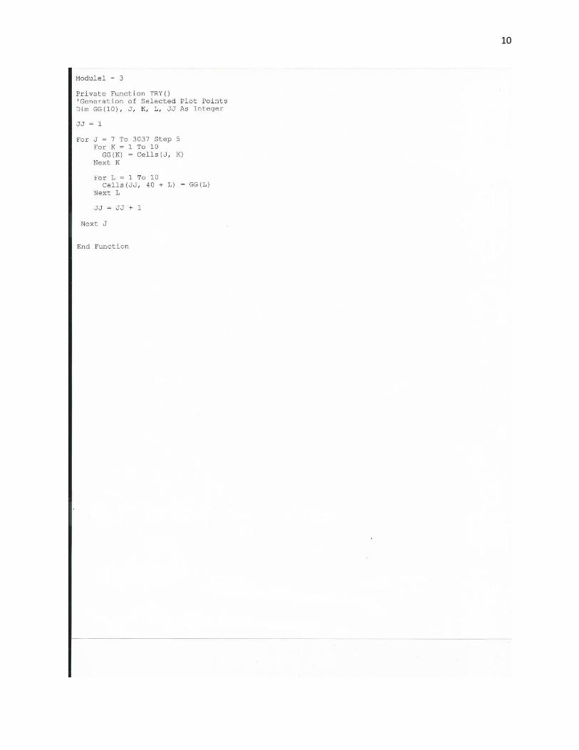
This small step size resulted in a large spreadsheet ( 3035 rows @ time = 15.17). The procedure TRY (Appendix I) was used to select a subset of data points for charting. A method of attaching a VBA file to a Word file is addressed in Appendix II.

References 1. http://en.wikipedia.org/wiki/Burgers%27_equation 2. Schiesser, W. E. , The Numerical Method of Lines – Integration of Partial Differential Equations , Academic Press, 1991 3. Biazar, J., Z.Ayati and S. Shahbazi , “Solution of the Burgers Equation by the Method of Lines”, American Journal of Numerical Analysis 2014 2 (1) pp 1-2 4. Nguyen, Vinh Q. ,” A Numerical Study of Burgers’ Equation With Robin Boundary Conditions”, Master of Science Thesis, Virginia Tech 5. Handi, S., W.E.Schiesser and G.W.Griffiths, “Method of Lines” http://www.scholarpedia.org/ 6. Sadiku, M.N.O. and C.N.Obizor, ”A simple introduction to the Method of lines”, International Journal of Electrical Engineering Education, Vol. 37, No 3. 7. http://web.engr.illinois.edu/~heath/iem/pde/burgers/ 8. http://pauli.uni-muenster.de/tp/fileadmin/lehre/NumMethoden/WS1011/script1011.pdf

Appendix I

8

9

10

11

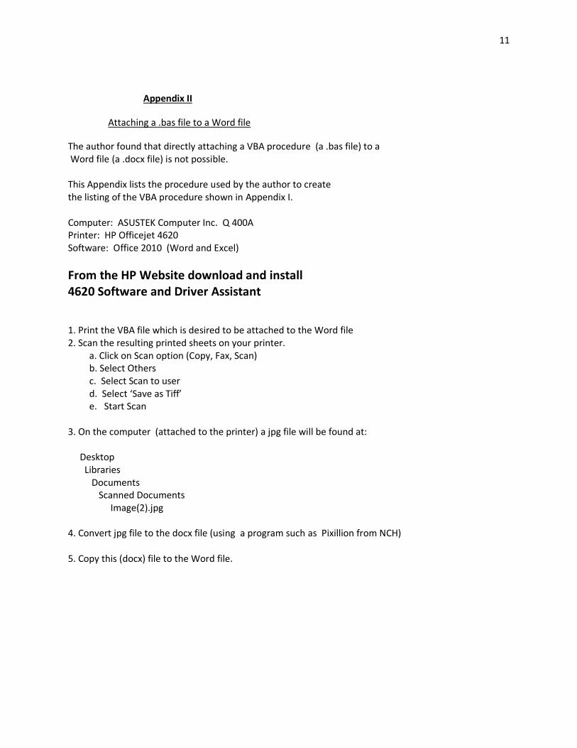
Appendix II

Attaching a .bas file to a Word file

The author found that directly attaching a VBA procedure (a .bas file) to a Word file (a .docx file) is not possible. This Appendix lists the procedure used by the author to create the listing of the VBA procedure shown in Appendix I. Computer: ASUSTEK Computer Inc. Q 400A Printer: HP Officejet 4620 Software: Office 2010 (Word and Excel)

From the HP Website download and install 4620 Software and Driver Assistant

1. Print the VBA file which is desired to be attached to the Word file 2. Scan the resulting printed sheets on your printer. a. Click on Scan option (Copy, Fax, Scan) b. Select Others c. Select Scan to user d. Select ‘Save as Tiff’ e. Start Scan 3. On the computer (attached to the printer) a jpg file will be found at: Desktop Libraries Documents Scanned Documents Image(2).jpg 4. Convert jpg file to the docx file (using a program such as Pixillion from NCH) 5. Copy this (docx) file to the Word file.