A Riemann-Hilbert Problem in a Riemann

Surface

Spyros Kamvissis

Department of Applied MathematicsUniversity of Crete, Greece

Euler Institute, August 19 2014

Toda lattice

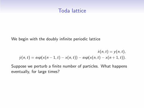
We begin with the doubly infinite periodic lattice

x(n, t) = y(n, t),

y(n, t) = exp(x(n − 1, t)− x(n, t)) − exp(x(n, t) − x(n + 1, t)).

Suppose we perturb a finite number of particles. What happenseventually, for large times?

Flaschka transformation and the Lax pair

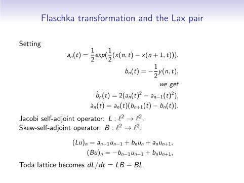
Setting

an(t) =1

2exp(

1

2(x(n, t) − x(n + 1, t))),

bn(t) = −1

2y(n, t),

we get

bn(t) = 2(an(t)2 − an−1(t)

2),

an(t) = an(t)(bn+1(t)− bn(t)).

Jacobi self-adjoint operator: L : ℓ2 → ℓ2.Skew-self-adjoint operator: B : ℓ2 → ℓ2.

(Lu)n = an−1un−1 + bnun + anun+1,

(Bu)n = −bn−1un−1 + bnun+1,

Toda lattice becomes dL/dt = LB − BL

Periodic Toda is explicitly solvablePeriodic Toda is explicitly solvable in terms of theta functions(Novikov, etc., Date-Tanaka 70s)There exist real numbers E0 < E1 < ........ < E2g+1

s.t.spec(L) = ∪gj=0[E2j ,E2j+1] (generically g + 1= period of

lattice).Let M be the Riemann surface associated with the function∏2g+1

j=0 (z − Ej ), g ∈ N. M is a compact, hyperelliptic Riemannsurface of genus g . Then

aper (n, t)2 = a2

θ(z(n + 1, t))θ(z(n − 1, t))

θ(z(n, t))2,

bper (n, t) = b +1

2

d

dtlog( θ(z(n, t))

θ(z(n − 1, t))

)

.

The constants a, b depend only on the Riemann surface, i.e. onE0 < E1 < · · · < E2g+1.Here θ(z) is the Riemann theta function associated with M andzℓ(n, t) = αℓ − nβℓ + tηℓ, where again αℓ, βℓ, ηℓ depend only onthe Riemann surface.

Theta function

θ(z) =∑

m∈Zg exp 2πi(

mz + mτ m2

)

, z ∈ Cg

Short Range Perturbation of Constant Background (K.1993)

Plot of a(., t) for three fixed consecutive times. Thebackground is: ast(n, 0) = 1, bst(n, 0) = 0

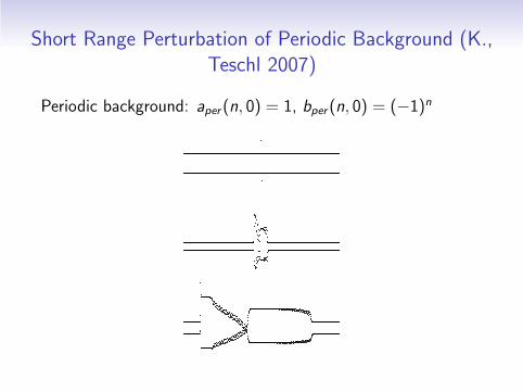
Short Range Perturbation of Periodic Background (K.,Teschl 2007)

Periodic background: aper (n, 0) = 1, bper (n, 0) = (−1)n

Explicit formulae

For long times the perturbed Toda lattice is asymptotically close tothe following limiting lattice:

∞∏

j=n

(alim(j , t)

aper (j , t))2 =

θ(z(n, t))

θ(z(n + 1, t))

θ(z(n + 1, t) + δ(n, t))

θ(z(n, t) + δ(n, t))×

× exp

(

1

2πi

∫

C(n/t)

log(1− |R |2)ω∞−∞+

)

,

δℓ(n, t) =1

2πi

∫

C (n/t)

log(1− |R |2)ζℓ,

zℓ(n, t) =αℓ − nβℓ + tηℓ,

where: θ Riemann theta function, ζℓ, ωpq Abelian differentials,C (n/t) contour depending on the stationary phase points of theRHP, αℓ, βℓ, ηℓ are functions of the spectrum (via Abel integrals),and R is the reflection coefficient of the perturbed lattice.

Numerical Comparison

Numerical comparison for genus one case, which can be computedin terms of elliptic functions:

Rieman-Hilbert factorization

The so-called nonlinear stationary − phase − steepest − descent

method for the asymptotic analysis of Rieman-Hilbert factorizationproblems has been very successful in providing(i) rigorous results on long time, long range and semiclassicalasymptotics for solutions of completely integrable equations andcorrelation functions of exactly solvable models,(ii) asymptotics for orthogonal polynomials of large degree,(iii) the limiting eigenvalue distribution of random matrices of largedimension (and thus universality results, i.e. independence of theexact distribution of the original entries, under some conditions),(iv) proofs of important results in combinatorial probability (e.g.the limiting distribution of the length of longest increasingsubsequence of a permutation, under uniform distribution).

Stationary phase

Even though the stationary phase idea was first applied to aRiemann-Hilbert problem and a nonlinear integrable equation byAlexander Its (1982) the method became systematic and rigorousin the work of Deift and Zhou (1993).In analogy to the linear stationary-phase and steepest-descentmethods, where one asymptotically reduces the given exponentialintegral to an exactly solvable one, in the nonlinear case oneasymptotically reduces the given Riemann-Hilbert problem to anexactly solvable one.

Non-self-adjointness

The term nonlinear steepest descent method is often used. Infact, there is a distinction between the stationary-phase idea andthe steepest-descent idea: actual steepest descent contours appearin non-self-adjoint problems.The distinction partly mirrors theself − adjoint/non − self − adjoint dichotomy of the underlyingLax operator;see Kamvissis K .McLaughlin Miller (2003)An extra feature appearing only in the nonlinear asymptotic theoryis the Lax − Levermore variational problem, discovered in 1979,before the work of Its, Deift and Zhou, but reappearing here in theguise of the so-called g − function which is catalytic in the processof deforming Riemann-Hilbert factorization problems to exactlysolvable ones.Non-self-adjoint case: Kamvissis Rakhmanov (2005)

THE LINEAR METHOD

Suppose one considers the Cauchy problem for, say, the linearizedKdVut − uxxx = 0.It can off course be solved via Fourier transforms. The end resultof the Fourier method is an exponential integral. To understandthe long time asymptotic behavior of the integral one needs toapply the stationary-phase method .The underlying principle, going back to Stokes and Kelvin, is thatthe dominating contribution comes from the vicinity of thestationary phase points. Through a local change of variables ateach stationary phase point and using integration by parts we cancalculate each contributing integral asymptotically to all orderswith exponential error. It is essential here that the phase xξ − ξ3tis real and that the stationary phase points are real.

Airy integralOn the other hand, suppose we have something like the Airyexponential integral

Ai(z) = 1π

∫

∞

0cos(s3/3 + zs)ds

and we are interested in z → ∞. Set s = z1/2t and x = z3/2. SoAi(x2/3) = x1/3

2π

∫

∞

−∞exp(ix(t3/3 + t))dt.

The phase is h(t) = t3

3 + t and the zeros of h′(t) = (t2+1) are ±i .As they are not real, before we apply any stationary-phase method,we have to deform the integral off the real line and along particularpaths: these are the steepest descent paths. They are given by thesimple characterization Imh(t) = constant. In our particularexample, the curves of steepest descent are the imaginary axis andthe two branches of a hyperbola. By deforming to one of thesebranches, we finally end up with Laplace type integrals and thenapply the same method as above (local change of variables plusintegration by parts) to recover valid asymptotics to all orders.

THE NONLINEAR METHOD

The nonlinear method generalizes the ideas above, but alsoemploys new ones.The analog of the Fourier transform is the scattering coefficientr(ξ) for the Jacobi operator: L : ℓ2 → ℓ2.

(Lu)n = an−1un−1 + bnun + anun+1

Scattering for the Decaying Case

Joukowski transformation

2λ = z + 1/z

The continuous spectrum [−1, 1] is mapped to the unit circle|z | = 1.This is convenient but also essential!

Scattering for the Decaying Case

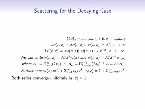
(Lu)n = an−1un−1 + bnun + anun+1

Lφ(n, z) = λφ(n, z); φ(n, z) ∼ zn, n → ∞

Lψ(n, z) = λψ(n, z); ψ(n, z) ∼ z−n, n → −∞.

We can write φ(n, z) = A+n z

nvn(z) and ψ(n, z) = A+n z

−nun(z)

where A+n = Π∞

k=n(2ak)−1, A−

n = Πn−1k=−∞(2ak)

−1 A = A+n A

−n .

Furthermore vn(z) = 1 + Σ∞n=1vn,kz

k , un(z) = 1 + Σ∞n=1un,kz

k .

Both series converge uniformly in |z | ≤ 1.

Scattering for the Decaying Case

On the other hand, when z 6= ±1,

φ(n, z), ψ(n, z) and φ(n, z−1), ψ(n, z−1)

are two sets of independent solutions of the second order differenceequation Lχ = λχ. Hence there exist A(z),B(z), α(z), β(z) suchthat

φ(n, z) = B(z)ψ(n, z) + A(z)ψ(n, z−1)

ψ(n, z) = β(z)φ(n, z) + α(z)φ(n, z−1)

z ∈ C , z 6= ±1.

We get

vn(z) =A−n

A+n

B(z)z−2nun(z) +A−n

A+n

A(z)un(z−1).

Scattering

Next define U1(n, z) = ψ(n, z), U2(n, z) =φ(n,z)A(z) = T (z)φ(n, z).

Since φ(n, z) ∼ A+n z

n and ψ(n, z) ∼ A−n z

−n near z = 0, we haveU1(n, z) ∼ A−

n z−n, U2(n, z) ∼ (A−

n )−1zn, near z = 0.

We end up with a Riemann-Hilbert problem

(

U+2 U+

1

)

=(

U−1 U−

2

)

(

1− |r(z)|2 −r(z)r(z) 1

)

with asymptotics(

U1 U2

)

∼(

A−n z

−n (A−n )

−1zn)

at z = 0and

(

U1 U2

)

∼(

A−n z

n (A−n )

−1z−n)

at infinity.

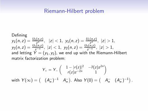
Riemann-Hilbert problem

Definingy1(n, z) =

U2(n,z)zn

, |z | < 1, y1(n, z) =U1(n,z)

zn, |z | > 1,

y2(n, z) =U1(n,z)z−n , |z | < 1, y2(n, z) =

U2(n,z)z−n , |z | > 1,

and letting Y = (y1, y2), we end up with the Riemann-Hilbertmatrix factorization problem:

Y+ = Y−

(

1− |r(z)|2 −r(z)z2n

r(z)z−2n 1

)

with Y (∞) =(

(A−n )

−1 A−n

)

. Also Y (0) =(

A−n (A−

n )−1)

.

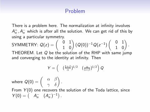
Problem

There is a problem here. The normalization at infinity involvesA+n ,A

−n which is after all the solution. We can get rid of this by

using a particular symmetry.

SYMMETRY: Q(z) =

(

0 11 0

)

(Q(0))−1Q(z−1)

(

0 11 0

)

.

THEOREM. Let Q be the solution of the RHP with same jumpand converging to the identity at infinity. Then

Y =(

( 1+βα )1/2 ( α

1+β )1/2)

Q

where Q(0) =

(

α βγ δ

)

.

From Y (0) one recovers the solution of the Toda lattice, sinceY (0) =

(

A−n (A−

n )−1)

.

Riemann-Hilbert Problem for the decaying Toda Lattice

Let r(z , 0) be the reflection coefficient for the initial data.Let Q be analytic off the unit circle and = I at infinity, with

Q+ = Q−

(

1− |r(z)|2 −r(z)z2nexp[(z − z−1) t2 ]r(z)z−2nexp[−(z − z−1) t2 ] 1

)

SetY =

(

( 1+βα )1/2 ( α

1+β )1/2)

Q

where Q(0) =

(

α βγ δ

)

.

Then Y (0) =(

A−n (A−

n )−1)

, and one recovers an from

A−n = Πn−1

k=−∞(2ak)

−1.

Stationary Phase Analysis

There are two stationary phase points zsp, z∗sp.

The Riemann-Hilbert Problem for the decaying Toda Lattice isreduced asymptotically to two factorization problems, theircontours being small crosses, centered at zsp, z

∗sp respectively,

that can be solved explicitly!!! in terms of parabolic cylinderfunctions.

cf. the linear stationary phase method, where the dominatingcontribution to an exponential integral comes from the vicinity ofthe stationary phase points.In fact, after some rescaling and approximating the ”local”integrals can be computed explicitly.Similar things happen here, although more technical.Approximating a Riemann-Hilbert Problem by another requiressome harmonic analysis and introducing some singular equations,equivalent to the given RHPs.

Important Observation

To make use of the symmetry one needs to use both copies of thespectral complex plane, that is both sheets of the underlyinghyperelliptic curve. In the case of genus zero, they can be mappedto the complex plane via the Joukowski transformation. This is nomore possible in thbe case of the periodic lattice with genusgreater than zero. We therefore need to postulate theRiemann-Hilbert problem on a Riemann surface.

Important Observation

The inverse scattering theory for the perturbed periodic lattice wasconstructed by Egorova-Michor-Teschl (2005). Jost functions aredefined as solution of the eigenvalue problem with asymptoticsdefined in terms of the Baker-Akhiezer functions of genus g.

limn→±∞

w(z)∓n(ψ±(z , n, t) − ψq,±(z , n, t)) = 0,

where w(z) is the quasimomentum map

w(z) = exp(

∫ p

E0

ω∞+,∞−

), p = (z ,+).

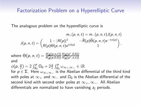
Factorization Problem on a Hyperelliptic Curve

The analogous problem on the hyperelliptic curve is

m+(p, n, t) = m−(p, n, t)J(p, n, t)

J(p, n, t) =

(

1− |R(p)|2 −R(p)Θ(p, n, t)e−tφ(p)

R(p)Θ(p, n, t)etφ(p) 1

)

,

where Θ(p, n, t) = θ(z(p,n,t))θ(z(p,0,0))

θ(z(p∗,0,0))θ(z(p∗,n,t))

andφ(p, n

t) = 2

∫ p

E0Ω0 + 2n

t

∫ p

E0ω∞+,∞−

∈ iR

for p ∈ Σ. Here ω∞+∞−is the Abelian differential of the third kind

with poles at ∞+ and ∞− and Ω0 is the Abelian differential of thesecond kind with second order poles at ∞+,∞−. All Abeliandifferentials are normalized to have vanishing aj periods.

Divisor Conditions

But m is NO MORE HOLOMORPHIC off the jump contour!The appropriate divisor condition is thatdiv(mj1) ≥ −divµ(n, t), div(mj2) ≥ −divµ∗(n, t), j = 1, 2where the poles are at the Dirichlet eigenvalues for the periodicproblem.Also we have bad conditions at the two infinities:m(∞+, n, t) =

(

A+(n, t)1

A+(n,t)

)

.

m(∞−, n, t) =(

1A+(n,t)

A+(n, t))

.

If we want to get rid of the bad condition at ∞+ then we need asymmetry. Then we can consider the normalized RHP and extractthe solution viaA+(n, t) =

√

1+(m12(∞−,n,t))(m11(∞−,n,t))

Stationary Phase Analysis

There are 2(g + 1) stationary phase points (g + 1 on each sheet)but only at most 2(1 on each sheet) in a band. So the others donot contribute (except an exponentially small error).Gaps correspond to a periodic asymptotics but bands correspondto a continuously modulated lattice.The geometry of the lenses is more delicate because of theRiemann surface background.Also the auxilliary scalar RHP has to be meromorphic, because ofthe Riemann-Roch theorem.

A generalized Cauchy kernel

In the complex plane, the solution of a Riemann–Hilbert problemcan be reduced to the solution of a singular integral equation. Inour case the underlying space is a Riemann surface. Hence wehave to replace the classical Cauchy kernel by a ”generalized”Cauchy kernel appropriate to our Riemann surface. In order to geta single valued kernel we need again to admit g poles. Allowingpoles at the nonspecial divisor div(µ) the corresponding Cauchykernel is given by

A generalized Cauchy kernel

Ωµp = ωp∞+ +

∑gj=1 Ij(p)ζj ,

where Ij (p) =∑g

l=1 cjl∫ p

∞+ωµl ,0,

ωq,0 is the Abelian differential of second kind with second orderpole at q and s.t.

∫

αkωq,0 = 0, all k

and ζj is a basis of holomorphic differentials.Note that Ij (p) has first order poles at the points µl .The constants cjl are chosen such that Ωp is single valued.

Connection with a Singular Integral EquationTHEOREM: Set

Ωµp =

(

Ωµp 0

0 Ωµ∗

p

)

and define the matrix operators as follows.

Given a 2x2 matrix f defined on Σ with Holder continuous entries,let(Cf )(p) = 1

π

∫

Σ f Ωp , for p 6∈ Σ, and (C±f )(q) = limp→q∈Σ(Cf )(p)from the left and right of Σ respectively (with respect to itsorientation). Then:1. The operators C± are given by the Plemelj formulas

(C+f )(q)− (C−f )(q) = f (q),

(C+f )(q) + (C−f )(q) =1

πPV

∫

Σ

fΩµq ,

and extend to bounded operators on L2(Σ).2. Cf is a meromorphic function off Σ, with divisor given by((Cf )j1) ≥ −div(µ) and ((Cf )j2) ≥ −div(µ∗).3. (Cf )(∞+) = 0.

Connection with a Singular Integral Equation

Now, given any b−, b+ ∈ L∞(Σ) with determinant equal to 1, letthe operator Cw : L2(Σ) → L2(Σ) be defined byCw f = C+(fw−) + C−(fw+) for a 2× 2 matrix valued f , wherew+ = b+ − I , and w− = I − b−.THEOREM. Assume that µ solves the singular integral equationµ = I + Cwµ in L2(Σ). Let Q be defined by the integral formulae

Q = I + C (µw), on M \ Σ,

where w = w+ + w−. Then Q is a solution of the followingmeromorphic Riemann–Hilbert problem.

Q+(p) = Q−(p)b−1− (p)b+(p), p ∈ Σ,

Q(∞+) = I ,

(Qj1) ≥ −div(µ), (Qj2) ≥ −div(µ∗).

References

S. Kamvissis, G. Teschl, Stability of Periodic Soliton Equationsunder Short Range Perturbations, Phys. Lett. A 364-6 (2007)Spyridon Kamvissis, Gerald Teschl, Long-time asymptotics of theperiodic Toda lattice under short-range perturbations, J.Math.Phys. 2012.

Helge Kruger, Gerald Teschl, Stability of the periodic Toda latticein the soliton region, Int. Math. Res. Not. 2009, Art. ID rnp077,36pp (2009).

Long-Time Asymptotics of Perturbed Finite-Gap Korteweg-deVries Solutions, Alice Mikikits-Leitner and Gerald Teschl, J.d’Analyse Math. 2012