A Robust Eigensolver for 3× 3 Symmetric Matrices

David Eberly, Geometric Tools, Redmond WA 98052https://www.geometrictools.com/

This work is licensed under the Creative Commons Attribution 4.0 International License. To view a copyof this license, visit http://creativecommons.org/licenses/by/4.0/ or send a letter to Creative Commons,PO Box 1866, Mountain View, CA 94042, USA.

Created: December 6, 2014Last Modified: September 20, 2016

Contents

1 Introduction 2

2 An Iterative Algorithm 2

3 A Variation of the Iterative Algorithm 3

4 Implementation of the Iterative Algorithm 5

5 A Noniterative Algorithm 10

5.1 Computing the Eigenvalues . . . . . . . . . . . . . . . . . . . . . . . . . . . . . . . . . . . . . 12

5.2 Computing the Eigenvectors . . . . . . . . . . . . . . . . . . . . . . . . . . . . . . . . . . . . . 14

6 Implementation of the Noniterative Algorithm 17

1

1 Introduction

Let A be a 3× 3 symmetric matrix of real numbers. From linear algebra, we know that A has all real-valuedeigenvalues and a full basis of eigenvectors. Let D = Diagonal(λ0, λ1, λ2) be the diagonal matrix whosediagonal entries are the eigenvalues. The eigenvalues are not necessarily distinct. Let R = [U0 U1 U2] bean orthogonal matrix whose columns are linearly independent eigenvectors, ordered consistently with thediagonal entries of D. That is, AUi = λiUi. The eigendecomposition is A = RDRT.

The typical presentation in a linear algebra class shows that the eigenvalues are the roots of the cubicpolynomial det(A− λI) = 0, where I is the 3× 3 identity matrix. The left-hand side of the equation is thedeterminant of the matrix A − λI. Closed-form equations exist for the roots of a cubic polynomial, so intheory one could compute the roots and for each one solve the equation (A− λI)U = 0 for nonzero vectorsU. Although correct theoretically, computing roots of the cubic polynomial using the closed-form equationsis known to be a non-robust algorithm (generally).

2 An Iterative Algorithm

A matrix M is specified by M = [mij ] for 0 ≤ i ≤ 2 and 0 ≤ 2. The classical numerical approach is touse a Householder reflection matrix H to compute B = HTAH so that b02 = 0; that is, B is a tridiagonalmatrix. The matrix H is a reflection, so HT = H. A sequence of Givens rotations Gk are used to drive thesuperdiagonal entries to zero. This is an iterative process for which a termination condition is required. Ifn rotations are applied, we obtain

GTn−1 · · ·GT

0HTAHG0 · · ·Gn−1 = D′ = D + E

where D′ is a tridiagonal matrix. The matrix D is diagonal and the matrix E has entries that are sufficientlysmall that the diagonal entries of D are reasonable approximations to the eigenvalues of A. The orthogonalmatrix R′ = HG0 · · ·Gn−1 has columns that are reasonable approximations to the eigenvectors of A.

The source code that implements this algorithm is in class SymmetricEigensolver found in the files

GeometricTools/GTEngine/Include/GteSymmetricEigensolver.{h, inl}

and is an implementation of Algorithm 8.2.3 (Symmetric QR Algorithm) described in Matrix Computations,2nd edition, by G. H. Golub and C. F. Van Loan, The Johns Hopkins University Press, Baltimore MD, FourthPrinting 1993. Algorithm 8.2.1 (Householder Tridiagonalization) is used to reduce matrix A to tridiagonalD′. Algorithm 8.2.2 (Implicit Symmetric QR Step with Wilkinson Shift) is used for the iterative reductionfrom tridiagonal to diagonal. Numerically, we have errors E = RTAR −D. Algorithm 8.2.3 mentions thatone expects |E| is approximately µ|A|, where |M | denotes the Frobenius norm of M and where µ is the unitroundoff for the floating-point arithmetic: 2−23 for float, which is FLT EPSILON = 1.192092896e-7f, and 2−52

for double, which is DBL EPSILON = 2.2204460492503131e-16.

The book uses the condition |a(i, i+1)| ≤ ε|a(i, i)+a(i+1, i+1)| to determine when the reduction decouplesto smaller problems. That is, when a superdiagonal term is effectively zero, the iterations may be appliedseparately to two tridiagonal submatrices. Our source code is implemented instead to deal with floating-pointnumbers,

2

sum = | a ( i , i ) | + | a ( i +1, i +1) | ;i f ( sum + | a ( i , i +1)| == sum){

// The s u p e r d i a g o n a l term a ( i , i +1) i s e f f e c t i v e l y z e r o .}

That is, the superdiagonal term is small relative to its diagonal neighbors, and so it is effectively zero. Theunit tests have shown that this interpretation of decoupling is effective.

3 A Variation of the Iterative Algorithm

The variation uses the Householder transformation to compute B = HTAH where b02 = 0. Let c = cos θand s = sin θ for some angle θ. The right-hand side is

HTAH =

c s 0

s −c 0

0 0 1

a00 a01 a02

a01 a11 a12

a02 a12 a22

c s 0

s −c 0

0 0 1

=

c2a00 + 2sca01 + s2a11 sc(a00 − a11) + (s2 − c2)a01 ca02 + sa12

sc(a00 − a11) + (s2 − c2)a01 c2a11 − 2sca01 + s2a00 sa02 − ca12ca02 + sa12 sa02 − ca12 a22

=

b00 b01 b02

b01 b11 b12

b02 b12 b22

We require 0 = b02 = ca02 + sa12 = (c, s) · (a02, a12), which occurs when (c, s) = (a12,−a02) /

√a202 + a212.

Rather than using Givens rotations for the iterations, we may instead use reflection matrices. Suppose that|b12| ≤ |b01|. We will choose a sequence of reflection matrices to drive b12 to zero. Choose a reflection matrix

G1 =

c1 0 −s1s1 0 c1

0 1 0

where c1 = cos θ1 and s1 = sin θ1 for some angle θ1. Consider the product

P1 = GT1BG1 =

c21b00 + 2s1c1b01 + s21b11 s1b12 s1c1(b11 − b00) + (c21 − s21)b01

s1b12 b22 c1b12

s1c1(b11 − b00) + (c21 − s21)b01 c1b12 c21b11 − 2s1c1b01 + s21b00

3

We need P1 to be tridiagonal, which requires

0 = s1c1(b11 − b00) + (c21 − s21)b01 = sin(2θ1)(b11 − b00)/2 + cos(2θ1)b01

leading us to two possible choices

(cos(2θ1), sin(2θ1)) = ± (b00 − b11, 2b01)√(b00 − b11)2 + 4b201

We must extract c1 = cos θ1 and s1 = sin θ from whichever solution we choose. In fact, we will choosecos(2θ1) ≤ 0 so that |c1| ≤ |s1| = s1. Let σ = Sign(b00 − b11); then

(cos(2θ1), sin(2θ1)) =(−|b00 − b11|,−2σb01)√

(b00 − b11)2 + 4b201, sin θ1 =

√1− cos(2θ1)

2, cos θ1 =

sin(2θ1)

2 sin θ1

Notice that| cos θ1| =

√(1 + cos(2θ1))/2 ≤

√(1− cos(2θ1))/2 = sin θ1

because we chose cos(2θ1) ≤ 0.

The previous construction guarantees that | cos θ0| ≤ 1/√

2 < 1. Let P1 = [p(1)ij ]; we now know p

(1)12 = c0b12,

so |p(1)12 | ≤ |b12|/√

2. Our precondition for computing P1 from B was that |b12| ≤ |b01|. A postcondition is

that |p(1)12 | = |c0b12| ≤ |s0b12| = |p(1)01 |, which is the precondition if we construct and multiply by anotherreflection G2 of the same form as G1.

Define P0 = B and let Pi+1 = GTi+1PiGi+1 be the iterative process. The conclusion is that the (1, 2)-entry

of the output matrix is smaller than the (1, 2)-entry of the input matrix, so indeed repeated iterations willdrive the (1, 2)-entry to zero. If ci = cos θi and si = sin θi, we have∣∣∣p(i+1)

12

∣∣∣ =∣∣∣ci+1p

(i)12

∣∣∣ ≤ 2−1/2∣∣∣p(i)12

∣∣∣which implies ∣∣∣p(i)12

∣∣∣ ≤ 2−i/2 |b12| , i ≥ 1

In the limit as i→∞, the (1, 2)-entry is forced to zero. In fact the bounds here allow you to select the finali so that 2−i/2|b12| is a number whose nearest floating-point representation is zero. The number of iterationsof the algorithm is limited by this i.

If instead we find that |b01| ≤ |b12|, we can choose the reflections to be of the form

Gi =

0 1 0

c1 0 s1

−s1 0 c1

Consider the product

P1 = GT1BG1 =

c21b11 − 2s1c1b12 + s21b22 c1b01 s1c1(b11 − b22) + (c21 − s21)b12

c1b01 b00 s1b01

s1c1(b11 − b22) + (c21 − s21)b12 s1b01 s21b11 + 2s1c1b12 + c21b22

4

Define σ = Sign(b22 − b11) and choose

(cos(2θ1), sin(2θ1)) =(−|b22 − b11|,−2σb12)√

(b22 − b11)2 + 4b212, sin θ1 =

√1− cos(2θ1)

2, cos θ1 =

sin(2θ1)

2 sin θ1

so that | cos θ1| =√

(1 + cos(2θ1))/2 ≤√

(1− cos(2θ1))/2 = sin θ1. We can apply the Gi to drive the(0, 1)-entry to zero.

A less aggressive approach is to use the condition mentioned previously that compares the superdiagonalentry to the diagonal entries using floating-point arithmetic.

4 Implementation of the Iterative Algorithm

The source code that implements the iterative algorithm for symmetric 3 × 3 matrices is in class Symmetri-

cEigensolver3x3 found in the file

GeometricTools/GTEngine/Include/GteSymmetricEigensolver3x3.h

The code was written not to use any GTEngine object. The class interface is

#inc l u d e <a l go r i t hm>#inc l u d e <a r ray>#inc l u d e <cmath>#inc l u d e < l i m i t s>

template <typename Real>c l a s s Symmet r i cE i g en so l v e r 3x3{pub l i c :

// The i npu t mat r i x must be symmetr ic , so on l y the un ique e l ement s must// be s p e c i f i e d : a00 , a01 , a02 , a11 , a12 , and a22 .//// I f ’ a g g r e s s i v e ’ i s ’ t r u e ’ , the i t e r a t i o n s occu r u n t i l a s u p e r d i a g o n a l// e n t r y i s e x a c t l y z e r o . I f ’ a g g r e s s i v e ’ i s ’ f a l s e ’ , the i t e r a t i o n s// occu r u n t i l a s u p e r d i a g o n a l e n t r y i s e f f e c t i v e l y z e r o compared to the// sum o f magni tudes o f i t s d i a g on a l n e i g hbo r s . G en e r a l l y , the// non ag g r e s s i v e conve rgence i s a c c e p t a b l e .//// The o r d e r o f the e i g e n v a l u e s i s s p e c i f i e d by so r tType : −1 ( d e c r e a s i n g ) ,// 0 ( no s o r t i n g ) , o r +1 ( i n c r e a s i n g ) . When so r t ed , the e i g e n v e c t o r s a r e// o rd e r ed a c c o r d i n g l y , and { evec [ 0 ] , evec [ 1 ] , evec [ 2 ]} i s gua ran teed to// be a r i g h t−handed or thono rma l s e t . The r e t u r n v a l u e i s the number o f// i t e r a t i o n s used by the a l g o r i t hm .

i n t ope ra to r ( ) ( Rea l a00 , Rea l a01 , Rea l a02 , Rea l a11 , Rea l a12 , Rea l a22 ,boo l a g g r e s s i v e , i n t sortType , s t d : : a r r ay<Real , 3>& eva l ,s t d : : a r r ay<s t d : : a r r ay<Real , 3>, 3>& evec ) const ;

p r i v a t e :// Update Q = Q∗G in−p l a c e u s i n g G = {{c ,0 ,− s } ,{ s , 0 , c } ,{0 ,0 ,1}} .vo id Update0 ( Rea l Q[ 3 ] [ 3 ] , Rea l c , Rea l s ) const ;

// Update Q = Q∗G in−p l a c e u s i n g G = {{0 ,1 ,0} ,{ c , 0 , s},{−s , 0 , c }} .vo id Update1 ( Rea l Q[ 3 ] [ 3 ] , Rea l c , Rea l s ) const ;

// Update Q = Q∗H in−p l a c e u s i n g H = {{c , s ,0} ,{ s ,−c , 0} ,{0 ,0 , 1}} .vo id Update2 ( Rea l Q[ 3 ] [ 3 ] , Rea l c , Rea l s ) const ;

// Update Q = Q∗H in−p l a c e u s i n g H = {{1 ,0 ,0} ,{0 , c , s } ,{0 , s ,−c }} .vo id Update3 ( Rea l Q[ 3 ] [ 3 ] , Rea l c , Rea l s ) const ;

5

// Norma l i ze (u , v ) r o bu s t l y , a v o i d i n g f l o a t i n g−po i n t o v e r f l ow i n the s q r t// c a l l . The no rma l i z ed p a i r i s ( cs , sn ) w i th cs <= 0 . I f ( u , v ) = (0 , 0 ) ,// the f u n c t i o n r e t u r n s ( cs , sn ) = (−1 ,0). When used to g en e r a t e a// Househo lde r r e f l e c t i o n , i t does not matte r whether ( cs , sn ) or (−cs ,− sn )// i s used . When g e n e r a t i n g a G ivens r e f l e c t i o n , c s = cos (2∗ t h e t a ) and// sn = s i n (2∗ t h e t a ) . Having a n e g a t i v e c o s i n e f o r the double−ang l e// term en s u r e s t ha t the s i n g l e−ang l e terms c = cos ( t h e t a ) and// s = s i n ( t h e t a ) s a t i s f y | c | <= | s | .vo id GetCosSin ( Rea l u , Rea l v , Rea l& cs , Rea l& sn ) const ;

// The conve rgence t e s t . When ’ a g g r e s s i v e ’ i s ’ t r u e ’ , the s u p e r d i a g o n a l// t e s t i s ” bSuper == 0” . When ’ a g g r e s s i v e ’ i s ’ f a l s e ’ , the s u p e r d i a g o n a l// t e s t i s ” | bDiag0 | + | bDiag1 | + | bSuper | == | bDiag0 | + | bDiag1 | , which// means bSuper i s e f f e c t i v e l y z e r o compared to the s i z e s o f the d i a g on a l// e n t r i e s .boo l Converged ( boo l a g g r e s s i v e , Rea l bDiag0 , Rea l bDiag1 ,

Rea l bSuper ) const ;

// Support f o r s o r t i n g the e i g e n v a l u e s and e i g e n v e c t o r s . The output// ( i0 , i1 , i 2 ) i s a pe rmuta t i on o f ( 0 , 1 , 2 ) so tha t d [ i 0 ] <= d [ i 1 ] <= d [ i 2 ] .// The ’ boo l ’ r e t u r n i n d i c a t e s whether the pe rmuta t i on i s odd . I f i t i s// not , the handedness o f the Q mat r i x must be ad j u s t e d .boo l Sor t ( s t d : : a r r ay<Real , 3> const& d , i n t& i0 , i n t& i1 , i n t& i 2 ) const ;

} ;

and the implementation is

template <typename Real>i n t Symmet r i cE igen so l v e r3x3<Real > : : ope ra to r ( ) ( Rea l a00 , Rea l a01 ,

Rea l a02 , Rea l a11 , Rea l a12 , Rea l a22 , boo l a g g r e s s i v e , i n t sortType ,s t d : : a r r ay<Real , 3>& eva l , s t d : : a r r ay<s t d : : a r r ay<Real , 3>, 3>& evec ) const

{// Compute the Househo lde r r e f l e c t i o n H and B = H∗A∗H, where b02 = 0 .Rea l const z e r o = ( Rea l )0 , one = ( Rea l )1 , h a l f = ( Rea l ) 0 . 5 ;boo l i s R o t a t i o n = f a l s e ;Rea l c , s ;GetCosSin ( a12 , −a02 , c , s ) ;Rea l Q [ 3 ] [ 3 ] = { { c , s , z e r o } , { s , −c , z e r o } , { zero , zero , one } } ;Rea l term0 = c ∗ a00 + s ∗ a01 ;Rea l term1 = c ∗ a01 + s ∗ a11 ;Rea l b00 = c ∗ term0 + s ∗ term1 ;Rea l b01 = s ∗ term0 − c ∗ term1 ;term0 = s ∗ a00 − c ∗ a01 ;term1 = s ∗ a01 − c ∗ a11 ;Rea l b11 = s ∗ term0 − c ∗ term1 ;Rea l b12 = s ∗ a02 − c ∗ a12 ;Rea l b22 = a22 ;

// G ivens r e f l e c t i o n s , B ’ = GˆT∗B∗G, p r e s e r v e t r i d i a g o n a l ma t r i c e s .i n t const max I t e r a t i o n = 2 ∗ (1 + s td : : n ume r i c l im i t s<Real > : : d i g i t s −

s t d : : n ume r i c l im i t s<Real > : : m in exponent ) ;i n t i t e r a t i o n ;Rea l c2 , s2 ;

i f ( s t d : : abs ( b12 ) <= std : : abs ( b01 ) ){

Rea l saveB00 , saveB01 , saveB11 ;f o r ( i t e r a t i o n = 0 ; i t e r a t i o n < max I t e r a t i o n ; ++i t e r a t i o n ){

// Compute the G ivens r e f l e c t i o n .GetCosSin ( h a l f ∗ ( b00 − b11 ) , b01 , c2 , s2 ) ;s = s q r t ( h a l f ∗ ( one − c2 ) ) ; // >= 1/ s q r t (2 )c = h a l f ∗ s2 / s ;

// Update Q by the G ivens r e f l e c t i o n .Update0 (Q, c , s ) ;i s R o t a t i o n = ! i s R o t a t i o n ;

// Update B <− QˆT∗B∗Q, e n s u r i n g tha t b02 i s z e r o and | b12 | has// s t r i c t l y d e c r e a s ed .

6

saveB00 = b00 ;saveB01 = b01 ;saveB11 = b11 ;term0 = c ∗ saveB00 + s ∗ saveB01 ;term1 = c ∗ saveB01 + s ∗ saveB11 ;b00 = c ∗ term0 + s ∗ term1 ;b11 = b22 ;term0 = c ∗ saveB01 − s ∗ saveB00 ;term1 = c ∗ saveB11 − s ∗ saveB01 ;b22 = c ∗ term1 − s ∗ term0 ;b01 = s ∗ b12 ;b12 = c ∗ b12 ;

i f ( Converged ( a g g r e s s i v e , b00 , b11 , b01 ) ){

// Compute the Househo lde r r e f l e c t i o n .GetCosSin ( h a l f ∗ ( b00 − b11 ) , b01 , c2 , s2 ) ;s = s q r t ( h a l f ∗ ( one − c2 ) ) ;c = h a l f ∗ s2 / s ; // >= 1/ s q r t (2 )

// Update Q by the Househo lde r r e f l e c t i o n .Update2 (Q, c , s ) ;i s R o t a t i o n = ! i s R o t a t i o n ;

// Update D = QˆT∗B∗Q.saveB00 = b00 ;saveB01 = b01 ;saveB11 = b11 ;term0 = c ∗ saveB00 + s ∗ saveB01 ;term1 = c ∗ saveB01 + s ∗ saveB11 ;b00 = c ∗ term0 + s ∗ term1 ;term0 = s ∗ saveB00 − c ∗ saveB01 ;term1 = s ∗ saveB01 − c ∗ saveB11 ;b11 = s ∗ term0 − c ∗ term1 ;break ;

}}

}e l s e{

Rea l saveB11 , saveB12 , saveB22 ;f o r ( i t e r a t i o n = 0 ; i t e r a t i o n < max I t e r a t i o n ; ++i t e r a t i o n ){

// Compute the G ivens r e f l e c t i o n .GetCosSin ( h a l f ∗ ( b22 − b11 ) , b12 , c2 , s2 ) ;s = s q r t ( h a l f ∗ ( one − c2 ) ) ; // >= 1/ s q r t (2 )c = h a l f ∗ s2 / s ;

// Update Q by the G ivens r e f l e c t i o n .Update1 (Q, c , s ) ;i s R o t a t i o n = ! i s R o t a t i o n ;

// Update B <− QˆT∗B∗Q, e n s u r i n g tha t b02 i s z e r o and | b12 | has// s t r i c t l y d e c r e a s ed . MODIFY . . .saveB11 = b11 ;saveB12 = b12 ;saveB22 = b22 ;term0 = c ∗ saveB22 + s ∗ saveB12 ;term1 = c ∗ saveB12 + s ∗ saveB11 ;b22 = c ∗ term0 + s ∗ term1 ;b11 = b00 ;term0 = c ∗ saveB12 − s ∗ saveB22 ;term1 = c ∗ saveB11 − s ∗ saveB12 ;b00 = c ∗ term1 − s ∗ term0 ;b12 = s ∗ b01 ;b01 = c ∗ b01 ;

i f ( Converged ( a g g r e s s i v e , b11 , b22 , b12 ) ){

// Compute the Househo lde r r e f l e c t i o n .GetCosSin ( h a l f ∗ ( b11 − b22 ) , b12 , c2 , s2 ) ;s = s q r t ( h a l f ∗ ( one − c2 ) ) ;

7

c = h a l f ∗ s2 / s ; // >= 1/ s q r t (2 )

// Update Q by the Househo lde r r e f l e c t i o n .Update3 (Q, c , s ) ;i s R o t a t i o n = ! i s R o t a t i o n ;

// Update D = QˆT∗B∗Q.saveB11 = b11 ;saveB12 = b12 ;saveB22 = b22 ;term0 = c ∗ saveB11 + s ∗ saveB12 ;term1 = c ∗ saveB12 + s ∗ saveB22 ;b11 = c ∗ term0 + s ∗ term1 ;term0 = s ∗ saveB11 − c ∗ saveB12 ;term1 = s ∗ saveB12 − c ∗ saveB22 ;b22 = s ∗ term0 − c ∗ term1 ;break ;

}}

}

s t d : : a r r ay<Real , 3> d i a g on a l = { b00 , b11 , b22 } ;i n t i 0 , i1 , i 2 ;i f ( so r tType >= 1){

// d i a g on a l [ i 0 ] <= d i a g on a l [ i 1 ] <= d i a g on a l [ i 2 ]boo l i sOdd = Sor t ( d i agona l , i0 , i1 , i 2 ) ;i f ( ! isOdd ){

i s R o t a t i o n = ! i s R o t a t i o n ;}

}e l s e i f ( so r tType <= −1){

// d i a g on a l [ i 0 ] >= d i a g on a l [ i 1 ] >= d i a g on a l [ i 2 ]boo l i sOdd = Sor t ( d i agona l , i0 , i1 , i 2 ) ;s t d : : swap ( i0 , i 2 ) ; // ( i0 , i1 , i 2 )−>( i2 , i1 , i 0 ) i s oddi f ( isOdd ){

i s R o t a t i o n = ! i s R o t a t i o n ;}

}e l s e{

i 0 = 0 ;i 1 = 1 ;i 2 = 2 ;

}

e v a l [ 0 ] = d i a g on a l [ i 0 ] ;e v a l [ 1 ] = d i a g on a l [ i 1 ] ;e v a l [ 2 ] = d i a g on a l [ i 2 ] ;evec [ 0 ] [ 0 ] = Q[ 0 ] [ i 0 ] ;evec [ 0 ] [ 1 ] = Q[ 1 ] [ i 0 ] ;evec [ 0 ] [ 2 ] = Q[ 2 ] [ i 0 ] ;evec [ 1 ] [ 0 ] = Q[ 0 ] [ i 1 ] ;evec [ 1 ] [ 1 ] = Q[ 1 ] [ i 1 ] ;evec [ 1 ] [ 2 ] = Q[ 2 ] [ i 1 ] ;evec [ 2 ] [ 0 ] = Q[ 0 ] [ i 2 ] ;evec [ 2 ] [ 1 ] = Q[ 1 ] [ i 2 ] ;evec [ 2 ] [ 2 ] = Q[ 2 ] [ i 2 ] ;

// Ensure the columns o f Q form a r i g h t−handed s e t .i f ( ! i s R o t a t i o n ){

f o r ( i n t j = 0 ; j < 3 ; ++j ){

evec [ 2 ] [ j ] = −evec [ 2 ] [ j ] ;}

}

r e t u r n i t e r a t i o n ;

8

}

template <typename Real>vo id Symmet r i cE igen so l v e r3x3<Real > : : Update0 ( Rea l Q[ 3 ] [ 3 ] , Rea l c , Rea l s ) const{

f o r ( i n t r = 0 ; r < 3 ; ++r ){

Rea l tmp0 = c ∗ Q[ r ] [ 0 ] + s ∗ Q[ r ] [ 1 ] ;Rea l tmp1 = Q[ r ] [ 2 ] ;Rea l tmp2 = c ∗ Q[ r ] [ 1 ] − s ∗ Q[ r ] [ 0 ] ;Q[ r ] [ 0 ] = tmp0 ;Q[ r ] [ 1 ] = tmp1 ;Q[ r ] [ 2 ] = tmp2 ;

}}

template <typename Real>vo id Symmet r i cE igen so l v e r3x3<Real > : : Update1 ( Rea l Q[ 3 ] [ 3 ] , Rea l c , Rea l s ) const{

f o r ( i n t r = 0 ; r < 3 ; ++r ){

Rea l tmp0 = c ∗ Q[ r ] [ 1 ] − s ∗ Q[ r ] [ 2 ] ;Rea l tmp1 = Q[ r ] [ 0 ] ;Rea l tmp2 = c ∗ Q[ r ] [ 2 ] + s ∗ Q[ r ] [ 1 ] ;Q[ r ] [ 0 ] = tmp0 ;Q[ r ] [ 1 ] = tmp1 ;Q[ r ] [ 2 ] = tmp2 ;

}}

template <typename Real>vo id Symmet r i cE igen so l v e r3x3<Real > : : Update2 ( Rea l Q[ 3 ] [ 3 ] , Rea l c , Rea l s ) const{

f o r ( i n t r = 0 ; r < 3 ; ++r ){

Rea l tmp0 = c ∗ Q[ r ] [ 0 ] + s ∗ Q[ r ] [ 1 ] ;Rea l tmp1 = s ∗ Q[ r ] [ 0 ] − c ∗ Q[ r ] [ 1 ] ;Q[ r ] [ 0 ] = tmp0 ;Q[ r ] [ 1 ] = tmp1 ;

}}

template <typename Real>vo id Symmet r i cE igen so l v e r3x3<Real > : : Update3 ( Rea l Q[ 3 ] [ 3 ] , Rea l c , Rea l s ) const{

f o r ( i n t r = 0 ; r < 3 ; ++r ){

Rea l tmp0 = c ∗ Q[ r ] [ 1 ] + s ∗ Q[ r ] [ 2 ] ;Rea l tmp1 = s ∗ Q[ r ] [ 1 ] − c ∗ Q[ r ] [ 2 ] ;Q[ r ] [ 1 ] = tmp0 ;Q[ r ] [ 2 ] = tmp1 ;

}}

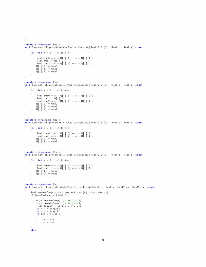
template <typename Real>vo id Symmet r i cE igen so l v e r3x3<Real > : : GetCosSin ( Rea l u , Rea l v , Rea l& cs , Rea l& sn ) const{

Rea l maxAbsComp = s td : : max( s td : : abs ( u ) , s t d : : abs ( v ) ) ;i f (maxAbsComp > ( Rea l )0 ){

u /= maxAbsComp ; // i n [−1 ,1]v /= maxAbsComp ; // i n [−1 ,1]Rea l l e n g t h = s q r t ( u∗u + v∗v ) ;c s = u / l e n g t h ;sn = v / l e n g t h ;i f ( c s > ( Rea l )0 ){

c s = −c s ;sn = −sn ;

}}e l s e

9

{c s = ( Rea l )−1;sn = ( Rea l ) 0 ;

}}

template <typename Real>boo l Symmet r i cE igen so l v e r3x3<Real > : : Converged ( boo l a g g r e s s i v e , Rea l bDiag0 , Rea l bDiag1 , Rea l bSuper ) const{

i f ( a g g r e s s i v e ){

r e t u r n bSuper == ( Rea l ) 0 ;}e l s e{

Rea l sum = std : : abs ( bDiag0 ) + s td : : abs ( bDiag1 ) ;r e t u r n sum + std : : abs ( bSuper ) == sum ;

}}

template <typename Real>boo l Symmet r i cE igen so l v e r3x3<Real > : : So r t ( s t d : : a r r ay<Real , 3> const& d , i n t& i0 , i n t& i1 , i n t& i 2 ) const{

boo l odd ;i f ( d [ 0 ] < d [ 1 ] ){

i f ( d [ 2 ] < d [ 0 ] ){

i 0 = 2 ; i 1 = 0 ; i 2 = 1 ; odd = t rue ;}e l s e i f ( d [ 2 ] < d [ 1 ] ){

i 0 = 0 ; i 1 = 2 ; i 2 = 1 ; odd = f a l s e ;}e l s e{

i 0 = 0 ; i 1 = 1 ; i 2 = 2 ; odd = t rue ;}

}e l s e{

i f ( d [ 2 ] < d [ 1 ] ){

i 0 = 2 ; i 1 = 1 ; i 2 = 0 ; odd = f a l s e ;}e l s e i f ( d [ 2 ] < d [ 0 ] ){

i 0 = 1 ; i 1 = 2 ; i 2 = 0 ; odd = t rue ;}e l s e{

i 0 = 1 ; i 1 = 0 ; i 2 = 2 ; odd = f a l s e ;}

}r e t u r n odd ;

}

5 A Noniterative Algorithm

An algorithm that is reasonably robust in practice is provided at the Wikipedia page Eigenvalue Algorithmin the section entitled 3 × 3 matrices. The algorithm involves converting a cubic polynomial to a formthat allows the application of a trigonometric identity in order to obtain closed-form expressions for the

10

roots. This topic is quite old; the Wikipedia page Cubic Function summarizes the history.1 Although thetopic is old, the current-day emphasis is usually the robustness of the algorithm when using floating-pointarithmetic. Knowing that real-valued symmetric matrices have only real-valued eigenvalues, we know thatthe characteristic cubic polynomial has roots that are all real valued. The Wikipedia discussion includespseudocode and a reference to a 1961 paper in the Communications of the ACM entitled Eigenvalues ofa symmetric 3 × 3 matrix. In my opinion, important details are omitted from the Wikipedia page. Inparticular, it is helpful to visualize the graph of the cubic polynomial det(βI − B) = β3 − 3β − det(B)in order to understand the location of the polynomial roots. This information is essential to computeeigenvectors when a real-valued root is repeated. The Wikipedia page mentions briefly the mathematicaldetails for generating the eigenvectors, but the discussion does not make it clear how to do so robustly in acomputer program.

I will use the notation that occurs at the Wikipedia page, except that the pseudocode will use 0-basedindexing of vectors and matrices rather than 1-based indexing. Let A be a real-valued symmetric 3 × 3matrix,

A =

a00 a01 a02

a01 a11 a12

a02 a12 a22

(1)

The trace of a matrix M , denoted tr(M), is the sum of the diagonal entries of M . The determinant of M isdenoted det(M). The characteristic polynomial for A is

f(α) = det(αI −A) = α3 − c2α2 + c1α− c0 (2)

where I is the 3× 3 identity matrix and where

c2 = a00 + a11 + a22 = tr(A)

c1 = (a00a11 − a201) + (a00a22 − a202) + (a11a22 − a212) =(tr2(A)− tr(A2)

)/2

c0 = a00a11a22 + 2a01a02a12 − a00a212 − a11a202 − a22a201 = det(A)

(3)

Given scalars p > 0 and q, define the matrix B by A = pB + qI. It is the case that A and B have thesame eigenvectors. If v is an eigenvector of A, then by definition Av = αv where α is an eigenvalue of A;moreover,

αv = Av = pBv + qv (4)

which implies Bv = ((α−q)/p)v. Thus, v is an eigenvector of B with corresponding eigenvalue β = (α−q)/p,or equivalently α = pβ + q. If we compute the eigenvalues and eigenvectors of B, we can then obtain theeigenvalues and eigenvectors of B.

1 My first exposure to the trigonometric approach was in high school when reading parts of my first-purchased mathematicsbook CRC Standard Mathematic Tables, the 19th edition published in 1971 by The Chemical Rubber Company. You mightrecognize the CRC acronym as part of CRC Press, a current-day publisher of books. The book title hides the fact that thereis quite a bit of (old) mathematics in the book. However, the book does have many tables of numbers because at the time thecommon tools for computing were (1) pencil and paper, (2) table lookups, and (3) a slide rule. Yes, I had my very own sliderule.

11

5.1 Computing the Eigenvalues

Define q = tr(A)/3 and p =√

tr ((A− qI)2) /6 so that B = (A− qI)/p. The Wikipedia discussion does notpoint out that this is defined only when p 6= 0. If A is a scalar multiple of the identity, then p = 0. On theother hand, the pseudocode at the Wikipedia page has special handling for when A is a diagonal matrix,which happens to include the case p = 0. The remainder of the construction here assumes p 6= 0. Somealgebraic manipulation will show that tr(B) = 0 and the characteristic polynomial is

g(β) = det(βI −B) = β3 − 3β − det(B) (5)

Choosing β = 2 cos(θ), the characteristic polynomial becomes

g(θ) = 2(4 cos3(θ)− 3 cos(θ)

)− det(B) (6)

Using the trigonometric identity cos(3θ) = 4 cos3(θ)− 3 cos(θ), we obtain

g(θ) = 2 cos(3θ)− det(B) (7)

The roots of g are obtained by solving for θ in the equation cos(3θ) = det(B)/2. Knowing that B has onlyreal-valued roots, it must be that θ is real-valued which implies | cos(3θ)| ≤ 1.2 This additionally impliesthat |det(B)| ≤ 2. The real-valued roots of g(θ) are

β = 2 cos

(θ +

2πk

3

), k = 0, 1, 2 (8)

where θ = arccos(det(B)/2)/3, and all roots are in the interval [−2, 2].

Let us now examine in greater detail the function g(β). The first derivative is g′(β) = 3β2− 3, which is zerowhen β = ±1. The second derivative is g′′(β) = 3β, which is not zero when g′(β) = 0. Therefore, β = −1produces a local maximum of g and β = +1 produces a local minimum of g. The graph of g has an inflectionpoint at β = 0 because g′′(0) = 0. A typical graph is shown in Figure 1.

2 When working with complex numbers, the magnitude of the cosine function can exceed 1.

12

Figure 1. The graph of g(β) = β3 − 3β − 1 where det(B) = 1. The graph was drawn usingMathematica (Wolfram Research, Inc., Mathematica, Version 11.0, Champaign, IL (2016)) but withmanual modifications to emphasize some key graph features.

The roots of g(β) are indeed in the interval [−2, 2]. Generally, g(−2) = g(1) = −2 − det(B), g(−1) =g(2) = 2− det(B), and g(0) = −det(B). Table 1 shows bounds for the roots. The roots are named so thatβ0 ≤ β1 ≤ β2.

Table 1. Bounds on the roots of g(β). The roots are ordered by β0 ≤ β1 ≤ β2.

det(B) > 0 θ + 2π/3 ∈ (2π/3, 5π/6) cos(θ + 2π/3) ∈ (−√

3/2,−1/2) β0 ∈ (−√

3,−1)

θ + 4π/3 ∈ (4π/3, 3π/2) cos(θ + 4π/3) ∈ (−1/2, 0) β1 ∈ (−1, 0)

θ ∈ (0, π/6) cos(θ) ∈ (√

3/2, 1) β2 ∈ (√

3, 2)

det(B) < 0 θ + 2π/3 ∈ (5π/6, π) cos(θ + 2π/3) ∈ (−1,−√

3/2) β0 ∈ (−2,−√

3)

θ + 4π/3 ∈ (3π/2, 5π/3) cos(θ + 4π/3) ∈ (0, 1/2) β1 ∈ (0, 1)

θ ∈ (π/6, π/3) cos(θ) ∈ (1/2,√

3/2) β2 ∈ (1,√

3)

det(B) = 0 θ + 2π/3 = 5π/6 cos(θ + 2π/3) = −√

3/2 β0 = −√

3

θ + 4π/3 = 3π/2 cos(θ + 4π/3) = 0 β1 = 0

θ = π/6 cos(θ) =√

3/2 β2 =√

3

Because tr(B) = 0, we also know β0 + β1 + β2 = 0.

13

Computing the eigenvectors for distinct and well-separated eigenvalues is generally robust. However, if a rootis repeated or two roots are nearly the same numerically, issues can occur when computing the 2-dimensionaleigenspace. Fortunately, the special form of g(β) leads to a robust algorithm.

5.2 Computing the Eigenvectors

The discussion here is based on constructing an eigenvector for β0 when β0 < 0 < β1 ≤ β2. The implementa-tion must also handle the construction of an eigenvector for β2 when β0 ≤ β1 < 0 < β2. The correspondingeigenvalues of A are α0, α1, and α2, ordered as α0 ≤ α1 ≤ α2. The eigenvectors for α0 are solutions to(A − α0I)v = 0. The matrix A − α0I is singular (by definition of eigenvalue) and in this case has rank 2;that is, two rows are linearly independent. Write the system of equations as shown next,

0

0

0

= 0 = (A− α0I)v =

rT0

rT1

rT2

v =

r0 · v

r1 · v

r2 · v

(9)

where ri are the 3× 1 vectors whose transposes are the rows of the matrix B − β0I. Assuming the first tworows are linearly independent, the conditions r0 ·v = 0 and r1 ·v = 0 imply v is perpendicular to both rows.Consequently, v is parallel to the cross product r0 × r1. We can normalize the cross product to obtain aunit-length eigenvector.

It is unknown which two rows of the matrix are linearly independent, so we must figure out which two rowsto choose. If two rows are nearly parallel, the cross product will have length nearly zero. For numericalrobustness, this suggests that we look at the three possible cross products of rows and choose the pair of rowsfor which the cross product has largest length. Alternatively, we could apply elementary row and columnoperations to reduce the matrix so that the last row is (numerically) the zero vector; this effectively is thealgorithm of using Gaussian elimination with full pivoting. In the pseudocode shown in Listing 1, the crossproduct approach is used.

Listing 1. Pseudocode for computing the eigenvector corresponding to the eigenvalue α0 of A that wasgenerated from the root β0 of the cubic polynomial for B that has multiplicity 1.

vo id ComputeEigenvector0 ( Matr i x3x3 A, Rea l e i g en va l u e0 , Vector3& e i g e n v e c t o r 0 ){

Vector3 row0 ( A(0 , 0 ) − e i g enva l u e0 , A(0 , 1 ) , A(0 , 2 ) ) ;Vector3 row1 ( A(0 , 1 ) , A(1 , 1 ) − e i g enva l u e0 , A(1 , 2 ) ) ;Vector3 row2 ( A(0 , 2 ) , A(1 , 2 ) , A(2 , 2 ) − e i g e n v a l u e 0 ) ;Vector3 r 0 x r 1 = Cros s ( row0 , row1 ) ;Vector3 r 0 x r 2 = Cros s ( row0 , row2 ) ;Vector3 r 1 x r 2 = Cros s ( row1 , row2 ) ;Rea l d0 = Dot ( r0x r1 , r 0 x r 1 ) ;Rea l d1 = Dot ( r0x r2 , r 0 x r 2 ) ;Rea l d2 = Dot ( r1x r2 , r 1 x r 2 ) ;Rea l dmax = d0 ;i n t imax = 0 ;i f ( d1 > dmax) { dmax = d1 ; imax = 1 ; }i f ( d2 > dmax) { imax = 2 ; }i f ( imax == 0){

e i g e n v e c t o r 0 = r0x r 1 / s q r t ( d0 ) ;}e l s e i f ( imax == 1)

14

{e i g e n v e c t o r 0 = r0x r 2 / s q r t ( d1 ) ;

}e l s e{

e i g e n v e c t o r 0 = r1x r 2 / s q r t ( d2 ) ;}

}

If the other two eigenvalues are well separated, the algorithm of Listing 1 may be used for each eigenvalue.However, if the two eigenvalues are nearly equal, Listing 1 can have numerical issues. The problem is thattheoretically when the eigenvalue is repeated (α1 = α2), the rank of A−α1I is 1. The cross products of anypair of rows is the zero vector. Determining the rank of a matrix numerically is problematic.

A different approach is used to compute an eigenvector of A − α1I. We know that the eigenvectors corre-sponding to α1 and α2 are perpendicular to the eigenvector W of α0. Compute unit-length vectors U andV such that {U,V,W} is a right-handed orthonormal set; that is, the vectors are all unit length, mutu-ally perpendicular, and W = U × V. The computations can be done robustly when using floating-pointarithmetic, as shown in Listing 2.

Listing 2. Robust computation of U and V for a specified W.

vo id ComputeOrthogonalComplement ( Vector3 W, Vector3& U, Vector3& V){

Rea l i nvLeng th ;i f ( f a b s (W[ 0 ] ) > f a b s (W[ 1 ] ) ){

// The component o f maximum ab s o l u t e v a l u e i s e i t h e r W[ 0 ] o r W[ 2 ] .i n vLeng th = 1 / s q r t (W[ 0 ] ∗ W[ 0 ] + W[ 2 ] ∗ W[ 2 ] ) ;U = Vector3(−W[ 2 ] ∗ i nvLength , 0 , +W[ 0 ] ∗ i n vLeng th ) ;

}e l s e{

// The component o f maximum ab s o l u t e v a l u e i s e i t h e r W[ 1 ] o r W[ 2 ] .i n vLeng th = 1 / s q r t (W[ 1 ] ∗ W[ 1 ] + W[ 2 ] ∗ W[ 2 ] ) ;U = Vector3 (0 , +W[ 2 ] ∗ i nvLength , −W[ 1 ] ∗ i n vLeng th ) ;

}Vector3 V = Cros s (W, U) ;

}

A unit-length eigenvector E of A−α1I must be a circular combination of U and V; that is, E = x0U+x1Vfor some choice of x0 and x1 with x20 + x21 = 1. There are exactly two such unit-length eigenvectors whenα1 6= α2 but infinitely many when α1 = α2.

Define the 3 × 2 matrix J = [U V] whose columns are the specified vectors. Define the 2 × 2 symmetricmatrix M = JT(A − α1I)J . Define the 2 × 1 vector X = JE whose rows are x0 and x1. The 3 × 3 linearsystem (A− α1I)E = 0 reduces to the 2× 2 linear system MX = 0. M has rank 1 when α1 6= α2, in whichcase M is not the zero matrix, or rank 0 when α1 = α2, in which case M is the zero matrix. Numerically,we need to trap the cases properly.

15

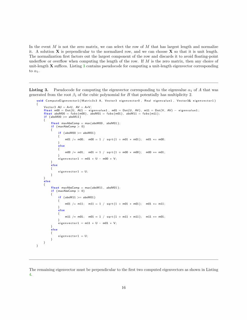
In the event M is not the zero matrix, we can select the row of M that has largest length and normalizeit. A solution X is perpendicular to the normalized row, and we can choose X so that it is unit length.The normalization first factors out the largest component of the row and discards it to avoid floating-pointunderflow or overflow when computing the length of the row. If M is the zero matrix, then any choice ofunit-length X suffices. Listing 3 contains pseudocode for computing a unit-length eigenvector correspondingto α1.

Listing 3. Pseudocode for computing the eigenvector corresponding to the eigenvalue α1 of A that wasgenerated from the root β1 of the cubic polynomial for B that potentially has multiplicity 2.

vo id ComputeEigenvector1 ( Matr i x3x3 A, Vector3 e i g e n v e c t o r 0 , Rea l e i g enva l u e1 , Vector3& e i g e n v e c t o r 1 ){

Vector3 AU = A∗U, AV = A∗V;f l o a t m00 = Dot (U, AU) − e i g enva l u e1 , m01 = Dot (U, AV) , m11 = Dot (V, AV) − e i g e n v a l u e 1 ;f l o a t absM00 = fab s (m00) , absM01 = fab s (m01) , absM11 = fab s (m11 ) ;i f ( absM00 >= absM11 ){

f l o a t maxAbsComp = max( absM00 , absM01 ) ;i f (maxAbsComp > 0){

i f ( absM00 >= absM01 ){

m01 /= m00 ; m00 = 1 / s q r t (1 + m01 ∗ m01 ) ; m01 ∗= m00 ;}e l s e{

m00 /= m01 ; m01 = 1 / s q r t (1 + m00 ∗ m00 ) ; m00 ∗= m01 ;}e i g e n v e c t o r 1 = m01 ∗ U − m00 ∗ V;

}e l s e{

e i g e n v e c t o r 1 = U;}

}e l s e{

f l o a t maxAbsComp = max( absM11 , absM01 ) ;i f (maxAbsComp > 0){

i f ( absM11 >= absM01 ){

m01 /= m11 ; m11 = 1 / s q r t (1 + m01 ∗ m01 ) ; m01 ∗= m11 ;}e l s e{

m11 /= m01 ; m01 = 1 / s q r t (1 + m11 ∗ m11 ) ; m11 ∗= m01 ;}e i g e n v e c t o r 1 = m11 ∗ U − m01 ∗ V;

}e l s e{

e i g e n v e c t o r 1 = U;}

}}

The remaining eigenvector must be perpendicular to the first two computed eigenvectors as shown in Listing4.

16

Listing 4. The remaining eigenvector is simply a cross product of the first two computed eigenvectors,and it is guaranteed to be unit length (within numerical tolerance).

ComputeEigenvector0 (A, e i g en va l u e0 , e i g e n v e c t o r 0 ) ;ComputeEigenvector1 (A, e i g e n v e c t o r 0 , e i g en va l u e1 , e i g e n v e c t o r 1 ) ;e i g e n v e c t o r 2 = Cros s ( e i g e n v e c t o r 0 , e i g e n v e c t o r 1 ) ;

6 Implementation of the Noniterative Algorithm

The source code that implements the iterative algorithm for symmetric 3× 3 matrices is in class NISymmet-

ricEigensolver3x3 found in the file

GeometricTools/GTEngine/Include/GteSymmetricEigensolver3x3.h

The code was written not to use any GTEngine object. The class interface is

#inc l u d e <a l go r i t hm>#inc l u d e <a r ray>#inc l u d e <cmath>#inc l u d e < l i m i t s>

template <typename Real>c l a s s NISymmet r i cE i g en so l v e r 3x3{pub l i c :

// The i npu t mat r i x must be symmetr ic , so on l y the un ique e l ement s must// be s p e c i f i e d : a00 , a01 , a02 , a11 , a12 , and a22 . The e i g e n v a l u e s a r e// s o r t e d i n a s c end i ng o r d e r : e v a l 0 <= eva l 1 <= eva l 2 .

vo id ope ra to r ( ) ( Rea l a00 , Rea l a01 , Rea l a02 , Rea l a11 , Rea l a12 , Rea l a22 ,s t d : : a r r ay<Real , 3>& eva l , s t d : : a r r ay<s t d : : a r r ay<Real , 3>, 3>& evec ) const ;

p r i v a t e :s t a t i c s t d : : a r r ay<Real , 3> Mu l t i p l y ( Rea l s , s t d : : a r r ay<Real , 3> const& U) ;s t a t i c s t d : : a r r ay<Real , 3> Sub t r a c t ( s t d : : a r r ay<Real , 3> const& U, s td : : a r r ay<Real , 3> const& V) ;s t a t i c s t d : : a r r ay<Real , 3> Div i d e ( s t d : : a r r ay<Real , 3> const& U, Rea l s ) ;s t a t i c Rea l Dot ( s t d : : a r r ay<Real , 3> const& U, s td : : a r r ay<Real , 3> const& V) ;s t a t i c s t d : : a r r ay<Real , 3> Cros s ( s t d : : a r r ay<Real , 3> const& U, s td : : a r r ay<Real , 3> const& V) ;

vo id ComputeOrthogonalComplement ( s t d : : a r r ay<Real , 3> const& W,s td : : a r r ay<Real , 3>& U, s td : : a r r ay<Real , 3>& V) const ;

vo id ComputeEigenvector0 ( Rea l a00 , Rea l a01 , Rea l a02 , Rea l a11 , Rea l a12 , Rea l a22 ,Rea l& eva l0 , s t d : : a r r ay<Real , 3>& evec0 ) const ;

vo id ComputeEigenvector1 ( Rea l a00 , Rea l a01 , Rea l a02 , Rea l a11 , Rea l a12 , Rea l a22 ,s t d : : a r r ay<Real , 3> const& evec0 , Rea l& eva l1 , s t d : : a r r ay<Real , 3>& evec1 ) const ;

} ;

and the implementation is

template <typename Real>vo id NISymmet r i cE igenso l v e r3x3<Real > : : ope ra to r ( ) ( Rea l a00 , Rea l a01 , Rea l a02 ,

Rea l a11 , Rea l a12 , Rea l a22 , s t d : : a r r ay<Real , 3>& eva l ,s t d : : a r r ay<s t d : : a r r ay<Real , 3>, 3>& evec ) const

{

17

// P r e c o nd i t i o n the mat r i x by f a c t o r i n g out the maximum ab s o l u t e v a l u e// o f the components . Th i s gua rds a g a i n s t f l o a t i n g−po i n t o v e r f l ow when// computing the e i g e n v a l u e s .Rea l max0 = s td : : max( f a b s ( a00 ) , f a b s ( a01 ) ) ;Rea l max1 = s td : : max( f a b s ( a02 ) , f a b s ( a11 ) ) ;Rea l max2 = s td : : max( f a b s ( a12 ) , f a b s ( a22 ) ) ;Rea l maxAbsElement = s td : : max( s td : : max(max0 , max1 ) , max2 ) ;i f ( maxAbsElement == ( Rea l )0 ){

// A i s the z e r o mat r i x .e v a l [ 0 ] = ( Rea l ) 0 ;e v a l [ 1 ] = ( Rea l ) 0 ;e v a l [ 2 ] = ( Rea l ) 0 ;evec [ 0 ] = { ( Rea l )1 , ( Rea l )0 , ( Rea l )0 } ;evec [ 1 ] = { ( Rea l )0 , ( Rea l )1 , ( Rea l )0 } ;evec [ 2 ] = { ( Rea l )0 , ( Rea l )0 , ( Rea l )1 } ;r e t u r n ;

}

Rea l invMaxAbsElement = ( Rea l )1 / maxAbsElement ;a00 ∗= invMaxAbsElement ;a01 ∗= invMaxAbsElement ;a02 ∗= invMaxAbsElement ;a11 ∗= invMaxAbsElement ;a12 ∗= invMaxAbsElement ;a22 ∗= invMaxAbsElement ;

Rea l norm = a01 ∗ a01 + a02 ∗ a02 + a12 ∗ a12 ;i f ( norm > ( Rea l )0 ){

// Compute the e i g e n v a l u e s o f A . The acos ( z ) f u n c t i o n r e q u i r e s | z | <= 1 ,// but w i l l f a i l s i l e n t l y and r e t u r n NaN i f the i n pu t i s l a r g e r than 1 i n// magnitude . To avo i d t h i s c o n d i t i o n due to round ing e r r o r s , the ha l fDe t// v a l u e i s clamped to [−1 ,1 ] .Rea l t r a c eD i v 3 = ( a00 + a11 + a22 ) / ( Rea l ) 3 ;Rea l b00 = a00 − t r a c eD i v 3 ;Rea l b11 = a11 − t r a c eD i v 3 ;Rea l b22 = a22 − t r a c eD i v 3 ;Rea l denom = sq r t ( ( b00 ∗ b00 + b11 ∗ b11 + b22 ∗ b22 + norm ∗ ( Rea l )2 ) / ( Rea l ) 6 ) ;Rea l c00 = b11 ∗ b22 − a12 ∗ a12 ;Rea l c01 = a01 ∗ b22 − a12 ∗ a02 ;Rea l c02 = a01 ∗ a12 − b11 ∗ a02 ;Rea l det = ( b00 ∗ c00 − a01 ∗ c01 + a02 ∗ c02 ) / ( denom ∗ denom ∗ denom ) ;Rea l h a l fDe t = det ∗ ( Rea l ) 0 . 5 ;h a l fDe t = s td : : min ( s td : : max( ha l fDet , ( Rea l )−1) , ( Rea l ) 1 ) ;

// The e i g e n v a l u e s o f B a r e o rd e r ed as beta0 <= beta1 <= beta2 . The// number o f d i g i t s i n twoTh i rd sP i i s chosen so that , whether f l o a t o r// double , the f l o a t i n g−po i n t number i s the c l o s e s t to t h e o r e t i c a l 2∗ p i /3 .Rea l ang l e = acos ( ha l fDe t ) / ( Rea l ) 3 ;Rea l const twoTh i rd sP i = ( Rea l )2 .09439510239319549 ;Rea l beta2 = cos ( ang l e ) ∗ ( Rea l ) 2 ;Rea l beta0 = cos ( ang l e + twoTh i rd sP i ) ∗ ( Rea l ) 2 ;Rea l beta1 = −(beta0 + beta2 ) ;

// The e i g e n v a l u e s o f A a r e o rd e r ed as a lpha0 <= alpha1 <= alpha2 .e v a l [ 0 ] = t r a c eD i v3 + denom ∗ beta0 ;e v a l [ 1 ] = t r a c eD i v3 + denom ∗ beta1 ;e v a l [ 2 ] = t r a c eD i v3 + denom ∗ beta2 ;

// The i ndex i 0 c o r r e s pond s to the r oo t gua ran teed to have m u l t i p l i c i t y 1// and goes w i th e i t h e r the maximum roo t or the minimum roo t . The i ndex// i 2 goes w i th the r oo t o f the o ppo s i t e ext reme . Root beta2 i s a lways// between beta0 and beta1 .i n t i 0 , i2 , i 1 = 1 ;i f ( h a l fDe t >= ( Rea l )0 ){

i 0 = 2 ;i 2 = 0 ;

}e l s e{

18

i 0 = 0 ;i 2 = 2 ;

}

// Compute the e i g e n v e c t o r s . The s e t { evec [ 0 ] , evec [ 1 ] , evec [ 2 ] } i s// r i g h t handed and or thono rma l .ComputeEigenvector0 ( a00 , a01 , a02 , a11 , a12 , a22 , e v a l [ i 0 ] , evec [ i 0 ] ) ;ComputeEigenvector1 ( a00 , a01 , a02 , a11 , a12 , a22 , evec [ i 0 ] , e v a l [ i 1 ] , evec [ i 1 ] ) ;evec [ i 2 ] = Cros s ( evec [ i 0 ] , evec [ i 1 ] ) ;

}e l s e{

// The mat r i x i s d i a g on a l .e v a l [ 0 ] = a00 ;e v a l [ 1 ] = a11 ;e v a l [ 2 ] = a22 ;evec [ 0 ] = { ( Rea l )1 , ( Rea l )0 , ( Rea l )0 } ;evec [ 1 ] = { ( Rea l )0 , ( Rea l )1 , ( Rea l )0 } ;evec [ 2 ] = { ( Rea l )0 , ( Rea l )0 , ( Rea l )1 } ;

}

// The p r e c o n d i t i o n i n g s c a l e d the mat r i x A, which s c a l e s the e i g e n v a l u e s .// Reve r t the s c a l i n g .e v a l [ 0 ] ∗= maxAbsElement ;e v a l [ 1 ] ∗= maxAbsElement ;e v a l [ 2 ] ∗= maxAbsElement ;

}

template <typename Real>s t d : : a r r ay<Real , 3> NISymmet r i cE igenso l v e r3x3<Real > : : Mu l t i p l y (

Rea l s , s t d : : a r r ay<Real , 3> const& U){

s t d : : a r r ay<Real , 3> product = { s ∗ U[ 0 ] , s ∗ U[ 1 ] , s ∗ U[ 2 ] } ;r e t u r n product ;

}

template <typename Real>s t d : : a r r ay<Real , 3> NISymmet r i cE igenso l v e r3x3<Real > : : Sub t r a c t (

s t d : : a r r ay<Real , 3> const& U, s td : : a r r ay<Real , 3> const& V){

s t d : : a r r ay<f l o a t , 3> d i f f e r e n c e = { U[ 0 ] − V[ 0 ] , U [ 1 ] − V[ 1 ] , U [ 2 ] − V [ 2 ] } ;r e t u r n d i f f e r e n c e ;

}

template <typename Real>s t d : : a r r ay<Real , 3> NISymmet r i cE igenso l v e r3x3<Real > : : D i v i d e (

s t d : : a r r ay<Real , 3> const& U, Rea l s ){

Rea l i nvS = ( Rea l )1 / s ;s t d : : a r r ay<Real , 3> d i v i s i o n = { U[ 0 ] ∗ invS , U [ 1 ] ∗ invS , U [ 2 ] ∗ i nvS } ;r e t u r n d i v i s i o n ;

}

template <typename Real>Rea l N ISymmet r i cE igenso l ve r3x3<Real > : : Dot ( s t d : : a r r ay<Real , 3> const& U,

s td : : a r r ay<Real , 3> const& V){

Rea l dot = U[ 0 ] ∗ V [ 0 ] + U[ 1 ] ∗ V [ 1 ] + U[ 2 ] ∗ V [ 2 ] ;r e t u r n dot ;

}

template <typename Real>s t d : : a r r ay<Real , 3> NISymmet r i cE igenso l v e r3x3<Real > : : C ro s s ( s t d : : a r r ay<Real , 3> const& U,

s td : : a r r ay<Real , 3> const& V){

s t d : : a r r ay<Real , 3> c r o s s ={

U[ 1 ] ∗ V [ 2 ] − U[ 2 ] ∗ V[ 1 ] ,U [ 2 ] ∗ V [ 0 ] − U[ 0 ] ∗ V[ 2 ] ,U [ 0 ] ∗ V [ 1 ] − U[ 1 ] ∗ V [ 0 ]

} ;r e t u r n c r o s s ;

19

}

template <typename Real>vo id NISymmet r i cE igenso l v e r3x3<Real > : : ComputeOrthogonalComplement (

s t d : : a r r ay<Real , 3> const& W, s td : : a r r ay<Real , 3>& U, s td : : a r r ay<Real , 3>& V) const{

// Robus t l y compute a r i g h t−handed or thono rma l s e t { U, V, W } . The// v e c t o r W i s gua ran teed to be un i t−l eng th , i n which ca se t h e r e i s no// need to worry about a d i v i s i o n by z e r o when computing i nvLeng th .Rea l i nvLeng th ;i f ( f a b s (W[ 0 ] ) > f a b s (W[ 1 ] ) ){

// The component o f maximum ab s o l u t e v a l u e i s e i t h e r W[ 0 ] o r W[ 2 ] .i n vLeng th = ( Rea l )1 / s q r t (W[ 0 ] ∗ W[ 0 ] + W[ 2 ] ∗ W[ 2 ] ) ;U = { −W[ 2 ] ∗ i nvLength , ( Rea l )0 , +W[ 0 ] ∗ i n vLeng th } ;

}e l s e{

// The component o f maximum ab s o l u t e v a l u e i s e i t h e r W[ 1 ] o r W[ 2 ] .i n vLeng th = ( Rea l )1 / s q r t (W[ 1 ] ∗ W[ 1 ] + W[ 2 ] ∗ W[ 2 ] ) ;U = { ( Rea l )0 , +W[ 2 ] ∗ i nvLength , −W[ 1 ] ∗ i n vLeng th } ;

}V = Cros s (W, U) ;

}

template <typename Real>vo id NISymmet r i cE igenso l v e r3x3<Real > : : ComputeEigenvector0 ( Rea l a00 , Rea l a01 ,

Rea l a02 , Rea l a11 , Rea l a12 , Rea l a22 , Rea l& eva l0 , s t d : : a r r ay<Real , 3>& evec0 ) const{

// Compute a un i t−l e n g t h e i g e n v e c t o r f o r e i g e n v a l u e [ i 0 ] . The mat r i x i s// rank 2 , so two o f the rows a r e l i n e a r l y i ndependen t . For a r obu s t// computat ion o f the e i g e n v e c t o r , s e l e c t the two rows whose c r o s s p roduc t// has l a r g e s t l e n g t h o f a l l p a i r s o f rows .s t d : : a r r ay<Real , 3> row0 = { a00 − eva l0 , a01 , a02 } ;s t d : : a r r ay<Real , 3> row1 = { a01 , a11 − eva l0 , a12 } ;s t d : : a r r ay<Real , 3> row2 = { a02 , a12 , a22 − e v a l 0 } ;s t d : : a r r ay<Real , 3> r 0 x r 1 = Cros s ( row0 , row1 ) ;s t d : : a r r ay<Real , 3> r 0 x r 2 = Cros s ( row0 , row2 ) ;s t d : : a r r ay<Real , 3> r 1 x r 2 = Cros s ( row1 , row2 ) ;Rea l d0 = Dot ( r0x r1 , r 0 x r 1 ) ;Rea l d1 = Dot ( r0x r2 , r 0 x r 2 ) ;Rea l d2 = Dot ( r1x r2 , r 1 x r 2 ) ;

Rea l dmax = d0 ;i n t imax = 0 ;i f ( d1 > dmax){

dmax = d1 ;imax = 1 ;

}i f ( d2 > dmax){

imax = 2 ;}

i f ( imax == 0){

evec0 = D i v i d e ( r0x r1 , s q r t ( d0 ) ) ;}e l s e i f ( imax == 1){

evec0 = D i v i d e ( r0x r2 , s q r t ( d1 ) ) ;}e l s e{

evec0 = D i v i d e ( r1x r2 , s q r t ( d2 ) ) ;}

}

template <typename Real>vo id NISymmet r i cE igenso l v e r3x3<Real > : : ComputeEigenvector1 ( Rea l a00 , Rea l a01 ,

Rea l a02 , Rea l a11 , Rea l a12 , Rea l a22 , s t d : : a r r ay<Real , 3> const& evec0 ,

20

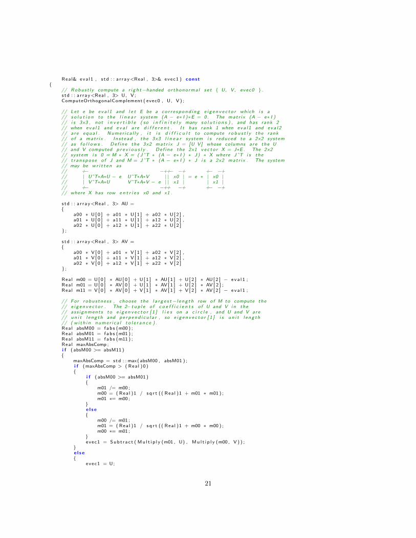
Rea l& eva l1 , s t d : : a r r ay<Real , 3>& evec1 ) const{

// Robus t l y compute a r i g h t−handed or thono rma l s e t { U, V, evec0 } .s t d : : a r r ay<Real , 3> U, V ;ComputeOrthogonalComplement ( evec0 , U, V ) ;

// Let e be e v a l 1 and l e t E be a c o r r e s p ond i n g e i g e n v e c t o r which i s a// s o l u t i o n to the l i n e a r system (A − e∗ I )∗E = 0 . The mat r i x (A − e∗ I )// i s 3x3 , not i n v e r t i b l e ( so i n f i n i t e l y many s o l u t i o n s ) , and has rank 2// when e v a l 1 and e v a l a r e d i f f e r e n t . I t has rank 1 when e v a l 1 and e v a l 2// a r e equa l . Numer i ca l l y , i t i s d i f f i c u l t to compute r o b u s t l y the rank// o f a mat r i x . I n s t e ad , the 3x3 l i n e a r system i s reduced to a 2x2 system// as f o l l o w s . De f i n e the 3x2 mat r i x J = [U V] whose columns a r e the U// and V computed p r e v i o u s l y . De f i n e the 2x1 v e c t o r X = J∗E . The 2x2// system i s 0 = M ∗ X = ( JˆT ∗ (A − e∗ I ) ∗ J ) ∗ X where JˆT i s the// t r a n s p o s e o f J and M = JˆT ∗ (A − e∗ I ) ∗ J i s a 2x2 mat r i x . The system// may be w r i t t e n as// +− −++− −+ +− −+// | UˆT∗A∗U − e UˆT∗A∗V | | x0 | = e ∗ | x0 |// | VˆT∗A∗U VˆT∗A∗V − e | | x1 | | x1 |// +− −++ −+ +− −+// where X has row e n t r i e s x0 and x1 .

s t d : : a r r ay<Real , 3> AU ={

a00 ∗ U[ 0 ] + a01 ∗ U[ 1 ] + a02 ∗ U[ 2 ] ,a01 ∗ U[ 0 ] + a11 ∗ U[ 1 ] + a12 ∗ U[ 2 ] ,a02 ∗ U[ 0 ] + a12 ∗ U[ 1 ] + a22 ∗ U[ 2 ]

} ;

s t d : : a r r ay<Real , 3> AV ={

a00 ∗ V [ 0 ] + a01 ∗ V [ 1 ] + a02 ∗ V[ 2 ] ,a01 ∗ V [ 0 ] + a11 ∗ V [ 1 ] + a12 ∗ V[ 2 ] ,a02 ∗ V [ 0 ] + a12 ∗ V [ 1 ] + a22 ∗ V [ 2 ]

} ;

Rea l m00 = U[ 0 ] ∗ AU[ 0 ] + U[ 1 ] ∗ AU[ 1 ] + U[ 2 ] ∗ AU[ 2 ] − e v a l 1 ;Rea l m01 = U[ 0 ] ∗ AV[ 0 ] + U[ 1 ] ∗ AV[ 1 ] + U[ 2 ] ∗ AV [ 2 ] ;Rea l m11 = V [ 0 ] ∗ AV[ 0 ] + V [ 1 ] ∗ AV[ 1 ] + V [ 2 ] ∗ AV[ 2 ] − e v a l 1 ;

// For r obu s tn e s s , choose the l a r g e s t−l e n g t h row o f M to compute the// e i g e n v e c t o r . The 2− t u p l e o f c o e f f i c i e n t s o f U and V i n the// a s s i gnmen t s to e i g e n v e c t o r [ 1 ] l i e s on a c i r c l e , and U and V a r e// u n i t l e n g t h and p e r p e nd i c u l a r , so e i g e n v e c t o r [ 1 ] i s u n i t l e n g t h// ( w i t h i n nume r i c a l t o l e r a n c e ) .Rea l absM00 = fab s (m00 ) ;Rea l absM01 = fab s (m01 ) ;Rea l absM11 = fab s (m11 ) ;Rea l maxAbsComp ;i f ( absM00 >= absM11 ){

maxAbsComp = s td : : max( absM00 , absM01 ) ;i f (maxAbsComp > ( Rea l )0 ){

i f ( absM00 >= absM01 ){

m01 /= m00 ;m00 = ( Rea l )1 / s q r t ( ( Rea l )1 + m01 ∗ m01 ) ;m01 ∗= m00 ;

}e l s e{

m00 /= m01 ;m01 = ( Rea l )1 / s q r t ( ( Rea l )1 + m00 ∗ m00 ) ;m00 ∗= m01 ;

}evec1 = Sub t r a c t ( Mu l t i p l y (m01 , U) , Mu l t i p l y (m00 , V ) ) ;

}e l s e{

evec1 = U;

21

}}e l s e{

maxAbsComp = s td : : max( absM11 , absM01 ) ;i f (maxAbsComp > ( Rea l )0 ){

i f ( absM11 >= absM01 ){

m01 /= m11 ;m11 = ( Rea l )1 / s q r t ( ( Rea l )1 + m01 ∗ m01 ) ;m01 ∗= m11 ;

}e l s e{

m11 /= m01 ;m01 = ( Rea l )1 / s q r t ( ( Rea l )1 + m11 ∗ m11 ) ;m11 ∗= m01 ;

}evec1 = Sub t r a c t ( Mu l t i p l y (m11 , U) , Mu l t i p l y (m01 , V ) ) ;

}e l s e{

evec1 = U;}

}}

22