a rule based missile evasion method for fighter aircrafts...

i

A RULE BASED MISSILE EVASION METHOD FOR FIGHTER AIRCRAFTS

A THESIS SUBMITTED TO THE GRADUATE SCHOOL OF NATURAL AND APPLIED SCIENCES

OF MIDDLE EAST TECHNICAL UNIVERSITY

BY

MUHAMMET SERT

IN PARTIAL FULLFILLMENT OF THE REQUIREMENTS FOR

THE DEGREE OF MASTER OF SCIENCE IN

ELECTRICAL AND ELECTRONICS ENGINEERING

MAY 2008

ii

Approval of the thesis:


submitted by MUHAMMET SERT in partial fulfillment of the requirements for

the degree of Master of Science in Electrical and Electronics Engineering

Department, Middle East Technical University by,

Prof. Dr. Canan Özgen

Dean, Graduate School of Natural and Applied Sciences

Prof. Dr. İsmet Erkmen

Head of Department, Electrical and Electronics Engineering

Prof. Dr. M. Kemal Leblebicioğlu

Supervisor, Electrical and Electronics Engineering Dept., METU

Examining Committee Members:

Prof. Dr. Mübeccel Demirekler

Electrical and Electronics Engineering Dept., METU Prof. Dr. M. Kemal Leblebicioğlu

Electrical and Electronics Engineering Dept., METU Prof. Dr. M. Kemal Özgören

Mechanical Engineering Dept., METU Assist. Prof. Dr. Afşar Saranlı

Electrical and Electronics Engineering Dept., METU Dr. Özgür Ateşoğlu

MGEO-MD-SGSM, ASELSAN

Date: 06.05.2008

iii

I hereby declare that all information in this document has been obtained and presented in accordance with academic rules and ethical conduct. I also declare that, as required by these rules and conduct, I have fully cited and referenced all material and results that are not original to this work.

Name, Last name : Muhammet Sert

Signature :

iv

ABSTRACT


Sert, Muhammet

M. Sc., Department of Electrical and Electronics Engineering

Supervisor: Prof. Dr. M. Kemal Leblebicioğlu

May 2008, 142 pages

In this thesis, a new guidance method for fighter aircrafts and a new guidance

method for missiles are developed. Also, guidance and control systems of the

aircraft and the missile used are designed to simulate the generic engagement

scenarios between the missile and the aircraft. Suggested methods have been tested

under excessive simulation studies.

The aircraft guidance method developed here is a rule based missile evasion

method. The main idea to develop this method stems from the maximization of the

miss distance for an engagement scenario between a missile and an aircraft. To do

this, an optimal control problem with state and input dependent inequality

constraints is solved and the solution method is applied on different problems that

represent generic scenarios. Then, the solutions of the optimal control problems are

used to extract rules. Finally, a method that uses the interpolation of the extracted

rules is given to guide the aircraft.

v

The new guidance method developed for missiles is formulated by modifying the

classical proportional navigation guidance method using the position estimates. The

position estimation is obtained by utilization of a Kalman based filtering method,

called interacting multiple models.

Keywords: Proportional Navigation Guidance, Optimal Control, Kalman Filter,

Interacting Multiple Models

vi

ÖZ

SAVAŞ UÇAKLARI İÇİN FÜZELERDEN KURAL TABANLI BİR KAÇMA YÖNTEMİ

Sert, Muhammet

Yüksek Lisans, Elektrik Elektronik Mühendisliği Bölümü

Tez Yöneticisi: Prof. Dr. M. Kemal Leblebicioğlu

Mayıs 2008, 142 sayfa

Bu tezde, savaş uçakları ve füzeler için birer yeni güdüm yöntemi geliştirilmiştir.

Ayrıca, füze ve uçak arasındaki jenerik angajman senaryolarının benzetimini

yapmak için, füze ve uçağın güdüm ve kontrol sistemleri tasarlanmıştır. Önerilen

yöntemler, benzetim çalışmaları ile yoğun bir şekilde test edilmiştir.

Uçak için geliştirilen güdüm yöntemi füzelerden kural tabanlı bir kaçma

yöntemidir. Füze ve uçak arasındaki bir angajman senaryosunda füzenin kaçırma

mesafesinin olabildiğince artırılması gereği, bu yöntemi geliştirmenin amacını

oluşturmaktadır. Bunun için, durum değişkenlerine ve girdilere bağlı eşitsizlik

sınırlamaları olan bir optimal kontrol problemi çözülerek, jenerik senaryoları temsil

eden birçok değişik durum için uygulanmıştır. Daha sonra, bu optimal kontrol

problemlerinin çözümlerinden yola çıkarak birtakım kurallar çıkarılmıştır. Son

olarak da, çıkarılan kuralları, ara değerleme yöntemi kullanarak uçağın güdüm

işlevini yerine getiren bir yöntem önerilmiştir.

vii

Füzeler için geliştirilen yeni güdüm yöntemi, klasik orantısal seyrüsefer güdüm

yönteminin, konum kestirim değerleri kullanılarak geliştirilmesiyle oluşturulmuştur.

Konum kestirimi ise, Kalman süzgeci tabanlı, etkileşimli çoklu model yöntemi ile

gerçekleştirilmiştir.

Anahtar Kelimeler: Orantısal Seyrüsefer Güdüm, Optimal Kontrol, Kalman

Süzgeci, Etkileşen Çoklu Modeller

viii

To My Family

and

My Darling

ix

ACKNOWLEDGMENTS

I would like to express my deepest gratitude to my supervisor Prof. Dr. M. Kemal

LEBLEBİCİOĞLU for his encouragement, guidance, advice, criticism and insight

throughout the research.

I wish to thank ASELSAN Inc. for facilities provided for the completion of this

thesis.

I am grateful to all of the thesis jury committee members who contributed to this

thesis with their valuable comments.

I would also like to express my profound appreciation to my family and my dear

girlfriend for their endless support, patience and understanding. Their love is the

meaning of life.

x

TABLE OF CONTENTS

ABSTRACT .........................................................................................................iv

ÖZ.........................................................................................................................vi

ACKNOWLEDGMENTS ...................................................................................ix

TABLE OF CONTENTS......................................................................................x

LIST OF TABLES ............................................................................................ xiii

LIST OF FIGURES ...........................................................................................xiv

LIST OF SYMBOLS AND ABBREVIATIONS..............................................xvii

CHAPTER 1 INTRODUCTION..........................................................................1

1.1 Thesis Outline .......................................................................................4

CHAPTER 2 FLIGHT DYNAMICS OF AN AIRCRAFT .................................6

2.1 Introduction...........................................................................................6

2.1.1 Coordinate Systems ........................................................................6

2.1.2 Assumptions .................................................................................10

2.2 Nonlinear EOM ...................................................................................11

2.2.1 Translational Dynamics ................................................................12

2.2.2 Rotational Dynamics.....................................................................14

2.2.3 Gathering the EOM.......................................................................15

2.2.4 Translational Dynamic Equations in WCS ....................................17

2.2.5 Nonlinear State-Space Model........................................................18

2.3 Trimming for the Steady-State Flight...................................................19

2.4 LTI State-Space Model........................................................................21

2.5 Decoupling of the State-Space Models.................................................23

xi

2.6 Flight Simulation.................................................................................25

CHAPTER 3 FLIGHT DYNAMICS OF A MISSILE ......................................27

3.1 Introduction.........................................................................................27

3.2 LTI State-Space Model........................................................................28

CHAPTER 4 AUTOPILOT OF THE AIRCRAFT...........................................30

4.1 Introduction.........................................................................................30

4.2 Linear Quadratic Controller (LQC) Design..........................................31

4.2.1 Linear Quadratic Regulator (LQR)................................................31

4.2.2 Selection of Quadratic Weights: Q and R......................................33

4.2.3 Suboptimal Linear Quadratic Tracker (SLQT) ..............................33

4.2.4 Gain Scheduling ...........................................................................38

4.2.5 Gain Scheduled LQC Design ........................................................42

4.2.6 Gain Scheduled LQC Design Performance....................................47

4.3 Proportional Integral Derivative (PID) Controller Design ....................49

4.3.1 PID Controller Design Example....................................................51

4.4 Comparison of LQC and PID Controller Performances........................56

CHAPTER 5 AUTOPILOT OF THE MISSILE ...............................................59

5.1 Introduction.........................................................................................59

5.2 Autopilot Design .................................................................................59

CHAPTER 6 GUIDANCE OF THE MISSILE .................................................63

6.1 Introduction.........................................................................................63

6.2 Proportional Navigation Guidance (PNG)............................................63

6.3 Proportional Integral Derivative Navigation Guidance (PIDNG)..........66

6.3.1 PIDNG Method Formulation.........................................................66

6.3.2 Parameter (kp, ki, kd) Selection......................................................67

6.4 Hybrid Proportional Navigation Guidance (HPNG) .............................70

6.4.1 CV Model.....................................................................................71

6.4.2 CA Model.....................................................................................72

6.4.3 IMM Filter Structure.....................................................................72

xii

6.4.4 Kalman Filter................................................................................75

6.4.5 Formulation of the HPNG Method ................................................77

6.5 Performance Comparison of the Guidance Methods.............................81

6.5.1 Scenarios ......................................................................................81

6.5.2 Simulation Results ........................................................................85

CHAPTER 7 GUIDANCE OF THE AIRCRAFT.............................................87

7.1 Introduction.........................................................................................87

7.2 Rule Based Missile Evasion Method....................................................88

7.2.1 Miss Distance Maximization as an Optimal Control Problem........88

7.2.2 Typical Engagement Scenarios .....................................................89

7.2.3 Interpolation Algorithm ..............................................................100

7.2.4 Implementation Details ...............................................................102

7.3 Anti-Proportional Navigation Guidance (Anti-PNG) .........................102

7.3.1 Formulation ................................................................................102

7.3.2 Conversion Logic........................................................................103

CHAPTER 8 SIMULATION STUDIES..........................................................106

CHAPTER 9 CONCLUSION AND FUTURE WORK...................................126

REFERENCES .................................................................................................129

APPENDIX A. AIRCRAFT DESIGN PARAMETERS..................................132

APPENDIX B. MISSILE DESIGN PARAMETERS ......................................141

xiii

LIST OF TABLES

TABLES

Table 2-1: System matrix, A, for the trim point given in Figure 4-3 ......................24

Table 2-2: Input matrix, B, for the trim point given in Figure 4-3..........................25

Table 4-1: Trim values of the state and the control variables .................................40

Table 4-2: Trim values of the state and the control variables – cont’d....................41

Table 4-3: Selection of Q and R for the longitudinal LQC design..........................44

Table 4-4: Longitudinal LQC design.....................................................................44

Table 4-5: Selection of Q and R for the lateral LQC design...................................46

Table 4-6: Lateral LQC design..............................................................................46

Table 6-1: Examples for PID parameter selection..................................................68

Table 6-2: Process noise levels for the CV and CA models used ...........................73

Table 6-3: Nest selection ........................................................................................78

Table 6-4: Initial conditions for the scenarios........................................................82

Table 6-5: Comparison of PIDNG and HPNG Methods ........................................86

Table 7-1: Engagement scenario parameters..........................................................92

Table 7-2: Engagement scenario parameters – cont’d............................................93

Table 7-3: Rules for the determination of the aircraft autopilot commands............99

Table 7-4: Rules for the determination of the aircraft autopilot commands – cont’d

.......................................................................................................................100

Table 8-1: Initial conditions of the test scenarios.................................................107

Table 8-2: Simulation results ..............................................................................107

Table A-1: Control surface actuator models [2]...................................................138

Table A-2: Other parameters used in the model...................................................139

Table A-3: Mass and geometry properties ...........................................................140

Table B-1: Control surface actuator models ........................................................141

xiv

LIST OF FIGURES

FIGURES

Figure 1-1: A generic homing type missile subsystems. ..........................................3

Figure 2-1: Earth-fixed, body, stability and wind coordinate systems ......................8

Figure 4-1: Servomechanism for a type 0 LTI system [1]. .....................................34

Figure 4-2: Servomechanism for a type 1 LTI system [1]. .....................................37

Figure 4-3: Trim points used for the controller design. ..........................................39

Figure 4-4: Block diagram used to test the performance of the autopilot designed for

an LTI system at a single trim point..................................................................42

Figure 4-5: Longitudinal autopilot of the aircraft designed with SLQT..................43

Figure 4-6: Lateral autopilot of the aircraft designed with SLQT...........................45

Figure 4-7: Height response of the LQC from the point A to the point B ...............47

Figure 4-8: Speed response of the LQC from the point A to the point B ................48

Figure 4-9: Yaw response of LQC from the point A to the point B........................48

Figure 4-10: Longitudinal autopilot of the aircraft designed with PID ...................49

Figure 4-11: Lateral autopilot of the aircraft designed with PID ............................50

Figure 4-12: Step response of the longitudinal autopilot for delta speed command 52

Figure 4-13: Step response of the longitudinal autopilot for delta height command53

Figure 4-14: Step response of the longitudinal autopilot after manual tuning - 1....54

Figure 4-15: Step response of the longitudinal autopilot after manual tuning – 2 ...54

Figure 4-16: Step response of the lateral autopilot for delta yaw command ...........55

Figure 4-17: Step response of the longitudinal autopilot for delta speed command 56

Figure 4-18: Step response of the longitudinal autopilot for delta height command57

Figure 4-19: Step response of the lateral autopilot for delta yaw command ...........57

Figure 5-1: Missile roll autopilot...........................................................................60

Figure 5-2: Missile normal acceleration autopilot..................................................61

Figure 5-3: Missile lateral acceleration autopilot ...................................................61

Figure 5-4: Unit step responses of the missile autopilots .......................................62

xv

Figure 6-1: Two-dimensional missile-target engagement geometry .......................64

Figure 6-2: Case 4.................................................................................................69

Figure 6-3: Case 7.................................................................................................69

Figure 6-4: Case 11...............................................................................................70

Figure 6-5: One cycle of the IMM Estimator [4]. ..................................................74

Figure 6-6: One cycle of the KF [4]. .....................................................................76

Figure 6-7: Measurement and estimation errors for S3, Nest=3.9, σw=1 m..............80

Figure 6-8: Measurement and estimation errors for S3, Nest=3.9, σw=5 m..............80

Figure 6-9: Measurement and estimation errors for S3, Nest=3.9, σw=10 m............81

Figure 6-10: Aircraft trajectories for S1, S2 and S3 – 1st view angle......................83

Figure 6-11: Aircraft trajectories for S1, S2 and S3 – 2nd view angle.....................84

Figure 6-12: Aircraft trajectories for S1, S2 and S3 – 3rd view angle .....................84

Figure 7-1: Missile and aircraft velocity vectors at the launch time .......................89

Figure 7-2: Generic engagement scenario for a missile and an aircraft - 1 .............90



Figure 7-5: Case 20, miss distance = 720 m ..........................................................96


Figure 7-7: Case 34, miss distance = 1208 m.........................................................97



Figure 7-10: Two-dimensional target-missile engagement geometry. ..................103

Figure 8-1: Anti-PNG method – case 1 ...............................................................109

Figure 8-2: Rule based method – case 1 ..............................................................109








Figure 8-10: Rule based method – case 5 ............................................................113

xvi

Figure 8-11: Anti-PNG method – case 6 .............................................................114








Figure 8-19: Anti-PNG method – case 10............................................................118

Figure 8-20: Rule based method – case 10 ..........................................................118















Figure A-1: Control surfaces of F-16...................................................................137

Figure B-1: Nonlinear control actuation system model........................................142

xvii

LIST OF SYMBOLS AND ABBREVIATIONS

Symbol Definition Unit

TV True air speed m/s

α Angle of attack deg

β Angle of sideslip deg

φ Roll angle deg

θ Pitch angle deg

ψ Yaw angle deg

p Body axis roll rate deg/s

q Body axis pitch rate deg/s

r Body axis yaw rate deg/s

Ex x-position w.r.t. earth fixed frame m

Ey y-position w.r.t. earth fixed frame m

Ez z-position w.r.t. earth fixed frame m

h Altitude w.r.t. earth fixed frame (h = -zE) m

pow Power setting (%) -

thδ Throttle setting (0-1) -

eδ Elevator setting deg

aδ Aileron setting deg

rδ Rudder setting deg

ρ Air density kg/m3

b Reference wing span m

c Mean aerodynamic chord m

TlC Total rolling moment coefficient -

TmC Total pitching moment coefficient -

TnC Total yawing moment coefficient -

TXC Total force coefficient along body x-axis -

xviii

Symbol Definition Unit

TYC Total force coefficient along body y-axis -

TZC Total force coefficient along body z-axis -

TF Total instantaneous engine thrust N

g Gravitational constant m/s2

engh Engine angular momentum kg.m2/s

xI Roll moment of inertia kg.m2

yI Pitch moment of inertia kg.m2

zI Yaw moment of inertia kg.m2

xzI Product moment of inertia kg.m2

xyI Product moment of inertia kg.m2

yzI Product moment of inertia kg.m2

L Rolling moment N.m

M Pitching moment N.m

N Yawing moment N.m

m Total aircraft mass kg

M Mach number -

sp Static pressure Pa

q Dynamic pressure Pa

S Reference wing area m2

T Temperature K

u Velocity component along body x-axis m/s

v Velocity component along body y-axis m/s

w Velocity component along body z-axis m/s

cgx Center of gravity location m

rcgx Reference center of gravity location m

X Body x-axis force component N

Y Body y-axis force component N

Z Body z-axis force component N

xix

Abbreviation Definition

1-D One Dimensional

3-D Three Dimensional

6-DOF Six Degrees of Freedom

BCS Body Coordinate System

CA Constant Acceleration

CAS Control Actuation System

CM Countermeasure

CCM Counter-Countermeasure

CV Constant Velocity

ECS Earth-fixed Coordinate System

EOM Equations of Motion

HPF High Pass Filter

HPNG Hybrid Proportional Navigation Guidance

HOT Higher Order Terms

IMM Interacting Multiple Models

IMM-KF Interacting Multiple Models - Kalman Filter

IR InfraRed

KF Kalman Filter

LOS Line of Sight

LPF Low Pass Filter

LQC Linear Quadratic Controller

LQR Linear Quadratic Regulator

LTI Linear Time Invariant

MIMO Multiple Input Multiple Output

NED North-East-Down

NL Nonlinear

PID Proportional-Integral-Derivative

PIDNG PID Navigation Guidance

PNG Proportional Navigation Guidance

RF Radio Frequency

xx

Abbreviation Definition

SCS Stability Coordinate System

SLQT Suboptimal Linear Quadratic Tracker

TM Transformation Matrix

UV Ultraviolet

WCS Wind Coordinate System

1

CHAPTER 1

INTRODUCTION

Modern electronic warfare necessitates the usage of intelligently guided missiles or

aircrafts since CM and CCM techniques are developing day by day. In a warfare

scenario, CM is a technique applied by the aircraft under missile threat. This

technique either requires dispensing of a convenient decoy creating a false target

that deceives the sensor of the missile, or an evasion maneuver that forces the

missile to reach its physical limits and hence no more able to track the aircraft.

In a real warfare environment, development of such CM and CCM techniques

require many trials by using the real systems that cost too much to design and

produce. However, verification and validation of effectiveness of a CM or a CCM

necessitates those high cost trials to collect data. In order not to make high cost

trials for every development phase of such techniques, modeling of the warfare

environment is done and then, the models are used on a software package that

simulates many possible scenarios by batch runs. If the modeling is successful to

represent the real world warfare scenario participants, such as a missile, an aircraft,

a CM, a CCM, the atmospheric effects, etc., then so many trials may be done by the

software with a low cost. Hence, collecting enough data by real trials in the field

gives way to verify and validate the models and so resulting in a very cost effective

way of developing new CM or CCM techniques.

2

In this thesis, some engagement scenarios between a missile and a fighter aircraft

are used to evaluate the effectiveness of the guidance models developed for both the

missile and the aircraft. If a real engagement between an IR guided SAM and a

fighter aircraft flying at low altitude with relatively low speed is considered, the

pilot must take a decision to guide the aircraft or apply a CM technique in such a

way that he/she can deceive the missile. The time to react for the pilot and the

range-to-go of the missile are the basic limitations that necessitate the usage of a

rule based or intelligent guidance system as soon as the threat is detected. As a

CCM technique, the missile may use a powerful tracking and guidance method that

discards the false targets created by flares. So, the result of the engagement depends

on both of the guidance methods used by the missile and the aircraft.

The development of the guidance models comes after the formulation of the flight

dynamics and implementation of the flight control systems. The derivation of the

flight dynamics and the implementation of the guidance and control systems require

some assumptions resulting in the approximate models that represent the real world

within an error bound. Effects that are neglected according to assumptions while

modeling of warfare scenario participants can be cited as aerodynamic coefficient

uncertainties, the change in the mass, inertia and the center of gravity, thrust

misalignment, change of the gravitational acceleration due to the instantaneous

position of the vehicle and atmospheric disturbance effects. In fact, all of these

factors affect the resultant state trajectory of the missile and the aircraft and so their

level of success changes.

A typical homing type IR guided missile can be modeled by designing seeker,

guidance, autopilot, CAS, airframe, rigid body dynamics and sensor subsystems that

are shown in the Figure 1-1. In this thesis, the seeker is not modeled as it is used in

a real missile system. Instead, the target position measurements are assumed to be

done. In some cases, in addition to the position measurements, position, velocity

and acceleration of the target are estimated by a tracker that is using interacting

multiple models via Kalman filtering. Then, measured or estimated position is used

3

to calculate the necessary inputs for the guidance subsystem. Also, the sensor

models used here are a standard first order low pass filters (LPFs) that are modeled

with a time constant. It is assumed that these sensors are able to measure every state

of the missile dynamical model that is shown as airframe in the Figure 1-1.

Figure 1-1: A generic homing type missile subsystems.

In the figure above, “missile information” represents the necessary states of the

missile itself to use in the guidance subsystem, and “target information” represents

the position information of the aircraft that is being tracked.

The states measured by the missile sensor are getting involved in the feedback loop

of the autopilot and also they are fed to the guidance subsystem. Since the measured

position of the missile fed to the guidance system is expressed in the BCS, it is

transformed into the ECS in order to calculate the necessary guidance commands in

this coordinate system. Then, these commands are transformed into the BCS and

passed to the acceleration limiter and hence, the limited acceleration commands are

used as the reference commands by the missile autopilot. The autopilot tracks the

reference acceleration commands and hence it creates desired fin deflection

4

commands to the CAS. The CAS is modeled as a first order system by using a time

constant value. Also, the CAS uses limitations for the demanded angles and rates so

that the real world physical saturations are simulated.

Modeling of the aircraft subsystems has some similarities, as well as differences

with the missile subsystems. The relative position of the missile with respect to the

aircraft is determined by a warning sensor in terms of either measuring the LOS

angles in azimuth and elevation and the range rate, or measuring the LOS rate in

azimuth and elevation and estimating the range rate. The former is done by using

RF sensors, whereas the latter is by IR or UV sensors. Also, the autopilot types used

for an aircraft may not be acceleration autopilots. Instead, desired-height, desired-

speed and desired-heading type autopilots may be used for the control of an aircraft.

These autopilots are also called flight path control systems [2], [3], [14]. The rest of

the subsystems can be modeled similar to the missile subsystems.

After briefly introducing the electronic warfare concept, the contents of the study is

outlined in the following section.

1.1 Thesis Outline

Chapter 2: This chapter explains the derivation of EOM of aircraft with the

necessary assumptions. First, the nonlinear EOM are derived. Then, the trim

conditions, trim process and linearization are explained. Lastly, the decoupling of

the state equations and brief information about the flight simulation of the aircraft

are given.

Chapter 3: In this chapter, flight dynamics of a missile is summarized based on the

study given in [13]. To do this, necessary assumptions are stated and the EOM of a

skid-to-turn type missile are given.

Chapter 4: Autopilots designed for the aircraft are explained. For lateral and

longitudinal autopilots, a classical control and a modern control technique are used.

5

The former is PID and the latter is LQR. By using these two techniques, local linear

controllers are designed at some trim points in the flight envelope of the aircraft.

Then, the control of nonlinear aircraft model is explained by using the local linear

controllers via gain scheduling, by using LQR technique. Consequently, the

performance results of these autopilot designs are given.

Chapter 5: In this chapter, the design of roll autopilot, normal acceleration and

lateral acceleration autopilots are formulated. Consequently, the performances of

these autopilots are illustrated.

Chapter 6: Applied missile guidance methods such as PNG, PIDNG and a new

guidance method named as HPNG are formulated and their performances while

tracking an aircraft are compared. The comparison method is based on three types

of flight maneuvers whose details are given in the last section of the chapter.

Chapter 7: A rule based missile evasion method is formulated in the first part of

this chapter. Then, a PNG based guidance (called anti-PNG) method is formulated

to evaluate the performance of the rule-based method by comparing the miss

distance obtained for some test scenarios that are given in chapter 8.

Chapter 8: Simulation studies to evaluate the performances of the proposed rule

based missile evasion method and the anti-PNG method are given in this chapter.

Also, the 3-D trajectories of the missile and the aircraft are given at the end of the

chapter.

Chapter 9: A brief summary about the work done throughout the thesis studies is

given as a conclusion and also some improvements are suggested as future work.

Appendix A: Modeling details of aerodynamics, engine, sensor, actuators and,

mass and geometry properties for a fighter aircraft (F-16) are explained.

Appendix B: Missile design parameters such as the sensor and the actuators are

given in this appendix.

6

CHAPTER 2

FLIGHT DYNAMICS OF AN AIRCRAFT

2.1 Introduction

In this chapter, nonlinear dynamical model of a fighter aircraft is derived.

Derivation is based on [6], [16], [2] and [3]. Mass and metric data of the aircraft are

given in Table A-3. Before getting into the detailed derivations, necessary

definitions of coordinate systems and assumptions are explained.

2.1.1 Coordinate Systems

There are many types of coordinate systems used for modeling and simulation of

aerospace vehicle dynamics. They are the inertial, the Earth, the geographic, the

local-level, the velocity, the body, the stability and the wind coordinate systems. In

this thesis, only four of these coordinate systems shown in Figure 2-1 are used to

derive the model of an aircraft and a missile to do 6-DOF flight simulations in 3-D.

Note that, all of the coordinate systems used are right handed. These coordinate

systems are described as follows:

Earth-fixed Coordinate System (ECS): XE and YE axes point to the North and

East directions respectively and they are located on a plane tangent to the Earth’s

surface. As a consequence, ZE axis points down to the center of the Earth, according

7

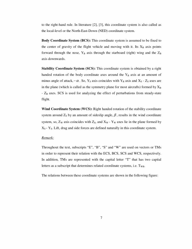
to the right-hand rule. In literature [2], [3], this coordinate system is also called as

the local-level or the North-East-Down (NED) coordinate system.

Body Coordinate System (BCS): This coordinate system is assumed to be fixed to

the center of gravity of the flight vehicle and moving with it. Its XB axis points

forward through the nose, YB axis through the starboard (right) wing and the ZB

axis downwards.

Stability Coordinate System (SCS): This coordinate system is obtained by a right

handed rotation of the body coordinate axes around the YB axis at an amount of

minus angle of attack, α− . So, YS axis coincides with YB axis and XS - ZS axes are

in the plane (which is called as the symmetry plane for most aircrafts) formed by XB

- ZB axes. SCS is used for analyzing the effect of perturbations from steady-state

flight.

Wind Coordinate System (WCS): Right handed rotation of the stability coordinate

system around ZS by an amount of sideslip angle, β , results in the wind coordinate

system, so, ZW axis coincides with ZS, and XW - YW axes lie in the plane formed by

XS - YS. Lift, drag and side forces are defined naturally in this coordinate system.

Remark:

Throughout the text, subscripts “E”, “B”, “S” and “W” are used on vectors or TMs

in order to represent their relation with the ECS, BCS, SCS and WCS, respectively.

In addition, TMs are represented with the capital letter “T” that has two capital

letters as a subscript that determines related coordinate systems, i.e. TWB.

The relations between these coordinate systems are shown in the following figure:

8

Figure 2-1: Earth-fixed, body, stability and wind coordinate systems

Coordinate TMs are used to transform a vector from one of the coordinate systems

to another. These TMs are orthogonal and also taking their transpose corresponds to

changing the sequence of transformation, i.e. BW

T

WB TT = . Another property of TMs

is that, consecutive transformations are contracted by canceling adjacent subscripts,

i.e. SWBSBW TTT = . For more properties, refer to [3].

The following TM is used to transform a vector expressed in ECS to BCS:

−+

+−

−

=

φθφψφθψφψφθψ

φθφψφθψφψφθψ

θθψθψ

coscossincoscossinsinsinsincossincos

sincoscoscossinsinsincossinsinsincos

sincossincoscos

BET , (2-1)

9

where, φ , θ and ψ are called roll, pitch and yaw angles that define the orientation

of the aircraft with respect to the ECS. These angles are known as Euler angles. In

fact, BET is formed by multiplication of three planar rotation matrices:

−

−

−

=

100

0cossin

0sincos

cos0sin

010

sin0cos

cossin0

sincos0

001

ψψ

ψψ

θθ

θθ

φφ

φφBET . (2-2)

It is apparent above that the sequence of the transformations is the yaw, pitch and

roll when transforming a vector from ECS to BCS and vice versa. Briefly, starting

from ECS, rotate about the ZE axis by yaw (nose right), then rotate about the new

Y-axis by pitch (nose up), and finally rotate about the new x-axis by roll (right wing

down). Note that all of these rotations are positive according to the right hand rule.

The TMs that define the relation between BCS, SCS and WCS are formed by angle

of attackα , and angle of sideslip β :

−

=

αα

αα

cos0sin

010

sin0cos

SBT , (2-3)

−=

100

0cossin

0sincos

ββ

ββ

WST . (2-4)

Since the transformation sequence between BCS and WCS

is WCSSCSBCS →→− βα , the TM that transforms a vector from BCS to WCS

is given as follows:

−

−−==

αα

βαββα

βαββα

cos0sin

sinsincossincos

cossinsincoscos

SBWSWB TTT . (2-5)

10

To define the angle of attack and sideslip, aircraft velocity vector components are

used as:

T

T

V

v

u

w

wvuV

arcsin

arctan

222

=

=

++=

β

α , (2-6)

where, VT is called as the true airspeed of the aircraft in BCS, and u, v and w are the

components of velocity vector of the aircraft in BCS. Especially, VT, α and β are

useful to express the aerodynamic force and moment coefficients when

multidimensional aerodynamic and thrust data look-up tables are given as function

of these variables [2].

2.1.2 Assumptions

A number of assumptions have to be made before proceeding with the derivation of

the EOM of the aircraft:

Assumption 1: The aircraft is a rigid body, which means that any two points on or

within the airframe remain fixed with respect to each other. Mass change due to fuel

consumption is neglected for the aircraft so its mass is taken as constant during the

flight. This assumption is necessary to apply Newton’s laws to derive the EOM.

Assumption 2: The Earth is flat and non-rotating and regarded as an inertial

reference (that is non-rotating and non-accelerating relative to the average position

of the fixed stars) [2]. This assumption is valid when dealing with the simulations of

aircraft and missiles that fly with speed below Mach 5 [3]. So, the ECS is used as an

inertial coordinate system for this flat Earth.

11

Assumption 3: Mass distribution of the aircraft is symmetric relative to the XB - ZB

plane of BCS, meaning that the products of inertia Iyz and Ixy are equal to zero. This

assumption is valid for most aircrafts.

Assumption 4: Angular momentum (heng) caused by the rotating machinery of the

aircraft engine is assumed to act along the positive x-axis of the BCS.

Assumption 5: The engine of the aircraft is mounted so that the thrust point lies on

the x-axis of the BCS.

Assumption 6: Gravity field is assumed to be uniform. In addition, the center of

mass and the center of gravity of the aircraft are coincident.

Assumption 7: Still atmosphere i.e. no winds, no gusts.

Under the assumptions above, motion of the aircraft has 6-DOF (rotation and

translation in three dimensions). The aircraft dynamics can be described by its

position, orientation, velocity and angular velocity over time.

2.2 Nonlinear EOM

The EOM for an aircraft can be derived from Newton’s 2nd Law of motion, which

states that the summation of all external forces acting on a body must be equal to

the time rate of change of its linear momentum relative to an inertial reference

frame, and the summation of all external moments acting on a body must be equal

to the time rate of change of its angular momentum relative to an inertial reference

frame. According to Assumption 2, Newton’s 2nd Law can be expressed in ECS by

two vector equations:

EVmdt

dF )(

rr= , (2-7)

EHdt

dM )(=r

, (2-8)

12

where, Fr

represents the sum of all externally applied forces, m is the mass of the

aircraft, Vr

is the velocity vector, Mr

represents the sum of all applied torques and

Hr

is the angular momentum. All of these four vectors are in BCS whereas the

derivative is taken with respect to the ECS. In order to take the derivative in the

BCS and express all the vectors in that coordinate system, Coriolis Theorem is used

[2]. This theorem states that derivative of a vector relative to one reference frame is

equal to derivative of the vector relative to a second reference frame plus cross

product of rotation vector of the second reference frame relative to the first

reference frame and the vector. For derivations of EOM, these two reference frames

are represented with the BCS and the ECS.

The force equation above is used to derive the translational dynamics, and the

moment equation is used to derive the rotational dynamics of the aircraft.

2.2.1 Translational Dynamics

Coriolis Theorem is applied to (2-7):

VmVmdt

dF B

rrrr×+= ω)( , (2-9)

where, ωr

is the angular velocity of the aircraft with respect to the ECS, expressed

in BCS. Formulating the vectors as the sum of their components with respect to the

BCS gives:

krjqip

kwjviuVrrrr

rrrr

++=

++=

ω, (2-10)

where, jirr

, and kr

are unit vectors along the aircraft’s body axes XB, YB and ZB,

respectively. Substituting (2-10) into (2-9) and considering Assumption 1 results

in:

13

)(

)(

)(

qupvwmF

pwruvmF

rvqwumF

z

y

x

−+=

−+=

−+=

&

&

&

, (2-11)

where, the external forces Fx, Fy and Fz depend on the weight vector Wr

, the

aerodynamic force vector Rr

and the thrust vector Tr

:

[ ] RWTFFFFT

zyx

rrrr++== . (2-12)

Thrust produced by the engine, FT, acts along aircraft’s XB-axis (Assumption 5),

which makes the thrust vector Tr

equal to:

[ ] [ ]T

T

T

zyx FTTTT 00==r

. (2-13)

Weight vector points to the center of the Earth, lying along the ZE axis of the ECS

and the aerodynamic force vector has the components in all axes of the BCS:

[ ] [ ]T

BE

T

zyx mgTWWWW 00==r

, (2-14)

[ ]TZYXR =

r, (2-15)

where, g is the gravity constant. In Appendix A.1 the aerodynamic forces X, Y and

Z are formulated by citing the effects that create these forces.

Hence, combining the last 4 equations results in the translational dynamic equations

in BCS:

)(coscos

)(cossin

)(sin

qupvwmmgZ

pwruvmmgY

rvqwummgFX T

−+=+

−+=+

−+=−+

&

&

&

θφ

θφ

θ

. (2-16)

14

2.2.2 Rotational Dynamics

Using Coriolis Theorem, (2-8) can be written as:

HHdt

dM B

rrrr×+= ω)( . (2-17)

In the BCS, under Assumption 1 and Assumption 4, angular momentum can be

expressed as:

[ ]TenghIH 00+= ωrr

, (2-18)

where, according to the Assumption 3, inertia matrix is defined as [2]:

−

−

=

zxz

y

xzx

II

I

II

I

0

00

0ˆ . (2-19)

Expanding (2-17) using (2-18) results in:

engxzxyxzzz

engxzzxyy

xzyzxzxx

qhqrIIIpqIpIrM

rhIrpIIprIqM

pqIIIqrIrIpM

−+−+−=

+−+−+=

−−+−=

)(

)()(

)(

22

&&

&

&&

, (2-20)

where, the external moments Mx, My and Mz are the components of Mr

along the

body coordinate axes. These moments are due to aerodynamics and thrust since

there is no moment caused by the gravity according to the Assumption 6. As a

result, the external moments are:

Tz

Ty

Tx

NNM

MMM

LLM

+=

+=

+=

, (2-21)

15

where, L , M and N are the aerodynamic moments and LT, MT and NT are the

moments due to the thrust. In Assumption 5, it is stated that there is no moment due

to thrust, so:

0=== TTT NML . (2-22)

Hence, combining (2-20) and (2-21), the rotational dynamic equations in BCS are

formed as:

engxzxyxzz

engxzzxy

xzyzxzx

qhqrIIIpqIpIrN

rhIrpIIprIqM

pqIIIqrIrIpL

−+−+−=

+−+−+=

−−+−=

)(

)()(

)(

22

&&

&

&&

. (2-23)

2.2.3 Gathering the EOM

In addition to the translational and rotational acceleration equations, two more

equations are needed to define the translational and rotational rates. These equations

formulate the transformation of the velocity vector Vr

from BCS to ECS and the

transformation of the angular velocity vector ωr

to the Euler rates [ ]Tψθφ &&& as

follows:

[ ] [ ]T

EB

T

EEE wvuTzyx =&&& , (2-24)

−=

r

q

p

θ

φ

θ

φφφ

φθφθ

ψ

θ

φ

cos

cos

cos

sin0

sincos0

costansintan1

&

&

&

, (2-25)

where, [ ]T

EEE zyx defines the position and [ ]Tψθφ defines the orientation

of the aircraft with respect to ECS.

16

The EOM derived up to here are now written as a system of 12 scalar first order

differential equations as follows:

Zm

gpvquw

Ym

grupwv

FXm

gqwrvu T

1coscos

1cossin

)(1

sin

++−=

++−=

++−−=

θφ

θφ

θ

&

&

&

, (2-26)

)()(

)()(

)()(

9428

722

65

4321

qhNcLcqrcpcr

rhMcrpcprcq

qhNcLcqpcrcp

eng

eng

eng

+++−=

−+−−=

++++=

&

&

&

, (2-27)

θ

φφψ

φφθ

φφθφ

cos

cossin

sincos

)cossin(tan

rq

rq

rqp

+=

−=

++=

&

&

&

, (2-28)

θφθφθ

ψφψθφψφψθφψθ

ψφψθφψφψθφψθ

coscoscossinsin

)cossinsinsin(cos)coscossinsin(sinsincos

)sinsincossin(sin)sincoscossin(sincoscos

wvuz

wvuy

wuux

E

E

E

++−=

−+++=

++−+=

&

&

&

, (2-29)

where, the moment of inertia components are given as [2]:

29623

2

2

8522

7242

2

1

)()(

1)(

xzzx

x

y

xz

xzzx

z

xzzx

xzyxx

y

xz

xzzx

xzzyx

yxzzx

xz

xzzx

xzzzy

III

Ic

I

Ic

III

Ic

III

IIIIc

I

IIc

III

IIIIc

Ic

III

Ic

III

IIIIc

−==

−=

−

+−=

−=

−

+−=

=−

=−

−−=

. (2-30)

17

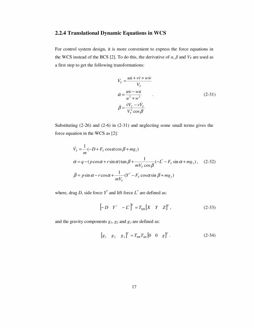
2.2.4 Translational Dynamic Equations in WCS

For control system design, it is more convenient to express the force equations in

the WCS instead of the BCS [2]. To do this, the derivative of α, β and VT are used as

a first step to get the following transformations:

ββ

α

cos2

22

T

TT

T

T

V

VvVv

wu

uwwu

V

wwvvuuV

&&&

&&&

&&&&

−=

+

−=

++=

. (2-31)

Substituting (2-26) and (2-6) in (2-31) and neglecting some small terms gives the

force equation in the WCS as [2]:

)sincos(1

cossin

)sin(cos

1tan)sincos(

)coscos(1

2*

3*

1

mgFYmV

rp

mgFLmV

rpq

mgFDm

V

T

T

T

T

TT

+−+−=

+−−++−=

++−=

βαααβ

αβ

βααα

βα

&

&

&

, (2-32)

where, drag D, side force Y* and lift force L* are defined as:

[ ] [ ]T

WB

TZYXTLYD =−− ∗∗ , (2-33)

and the gravity components g1, g2 and g3 are defined as:

[ ] [ ]T

BEWB

TgTTggg 00321 = . (2-34)

18

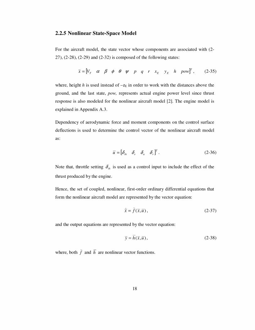
2.2.5 Nonlinear State-Space Model

For the aircraft model, the state vector whose components are associated with (2-

27), (2-28), (2-29) and (2-32) is composed of the following states:

[ ]T

EET powhyxrqpVx ψθφβα= , (2-35)

where, height h is used instead of –zE in order to work with the distances above the

ground, and the last state, pow, represents actual engine power level since thrust

response is also modeled for the nonlinear aircraft model [2]. The engine model is

explained in Appendix A.3.

Dependency of aerodynamic force and moment components on the control surface

deflections is used to determine the control vector of the nonlinear aircraft model

as:

[ ]T

raethu δδδδ= . (2-36)

Note that, throttle setting thδ is used as a control input to include the effect of the

thrust produced by the engine.

Hence, the set of coupled, nonlinear, first-order ordinary differential equations that

form the nonlinear aircraft model are represented by the vector equation:

),( uxfx =& , (2-37)

and the output equations are represented by the vector equation:

),( uxhy = , (2-38)

where, both f and h are nonlinear vector functions.

19

2.3 Trimming for the Steady-State Flight

In the theory of nonlinear systems, solution(s) of the following equation is (are)

defined as the equilibrium point(s) of the autonomous (with no external control

inputs) time-invariant system [2]:

),(0 eqeqeq uxfx ==& , (2-39)

where, equ is either zero or constant. At an equilibrium point, the system is said to

be “at rest” since the derivatives of all the variables are zero. As a result, behavior

of the system at rest is examined by slightly perturbing some of the variables. For

example, if the state trajectory of an aircraft departs rapidly from an equilibrium

point after a small perturbation of pitch attitude command given by a human pilot,

then control of the aircraft by the pilot is said to be improbable.

Steady-state flight for an aircraft is defined as a condition in which all linear and

angular velocity components are constant or zero, and all acceleration components

are zero [2]. In other words, in equilibrium or a steady-state condition, vector sum

of all the forces acting on the aircraft are equal to zero. Besides, the vector sum of

all the moments acting on the aircraft is equal to zero in an equilibrium condition,

which is also called as a trim condition.

The trim conditions for the nonlinear aircraft model used in this study are

formulated with the following equations:

[ ] 0=T

T rqpV &&&&&& βα , (2-40)

[ ] constT

raeth =δδδδ , (2-41)

[ ] 0=T

rqpφψθφ &&& . (2-42)

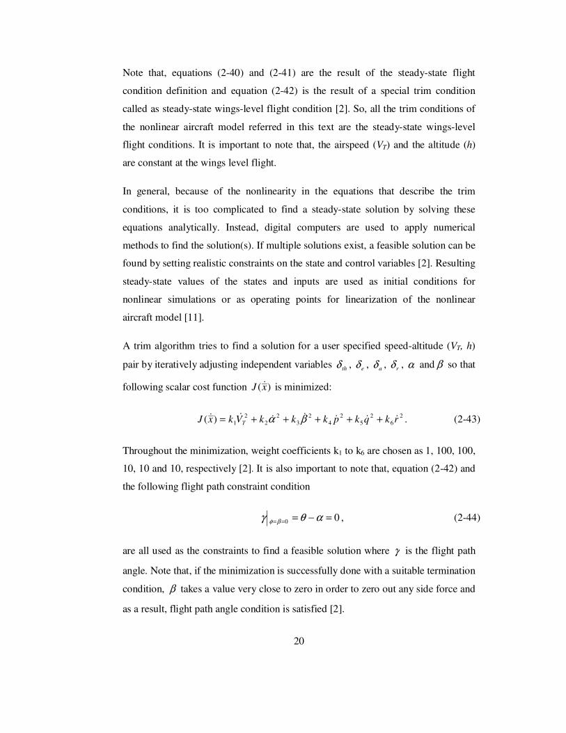
20

Note that, equations (2-40) and (2-41) are the result of the steady-state flight

condition definition and equation (2-42) is the result of a special trim condition

called as steady-state wings-level flight condition [2]. So, all the trim conditions of

the nonlinear aircraft model referred in this text are the steady-state wings-level

flight conditions. It is important to note that, the airspeed (VT) and the altitude (h)

are constant at the wings level flight.

In general, because of the nonlinearity in the equations that describe the trim

conditions, it is too complicated to find a steady-state solution by solving these

equations analytically. Instead, digital computers are used to apply numerical

methods to find the solution(s). If multiple solutions exist, a feasible solution can be

found by setting realistic constraints on the state and control variables [2]. Resulting

steady-state values of the states and inputs are used as initial conditions for

nonlinear simulations or as operating points for linearization of the nonlinear

aircraft model [11].

A trim algorithm tries to find a solution for a user specified speed-altitude (VT, h)

pair by iteratively adjusting independent variables thδ , eδ , aδ , rδ , α and β so that

following scalar cost function )(xJ & is minimized:

26

25

24

23

22

21)( rkqkpkkkVkxJ T

&&&&&&& +++++= βα . (2-43)

Throughout the minimization, weight coefficients k1 to k6 are chosen as 1, 100, 100,

10, 10 and 10, respectively [2]. It is also important to note that, equation (2-42) and

the following flight path constraint condition

00 =−=== αθγ βφ , (2-44)

are all used as the constraints to find a feasible solution where γ is the flight path

angle. Note that, if the minimization is successfully done with a suitable termination

condition, β takes a value very close to zero in order to zero out any side force and

as a result, flight path angle condition is satisfied [2].

21

For the minimization, simplex algorithm is used as the multivariable numerical

optimization algorithm since it performs well on this problem [2]. Details and

implementation of this algorithm can be found in [2] and [8].

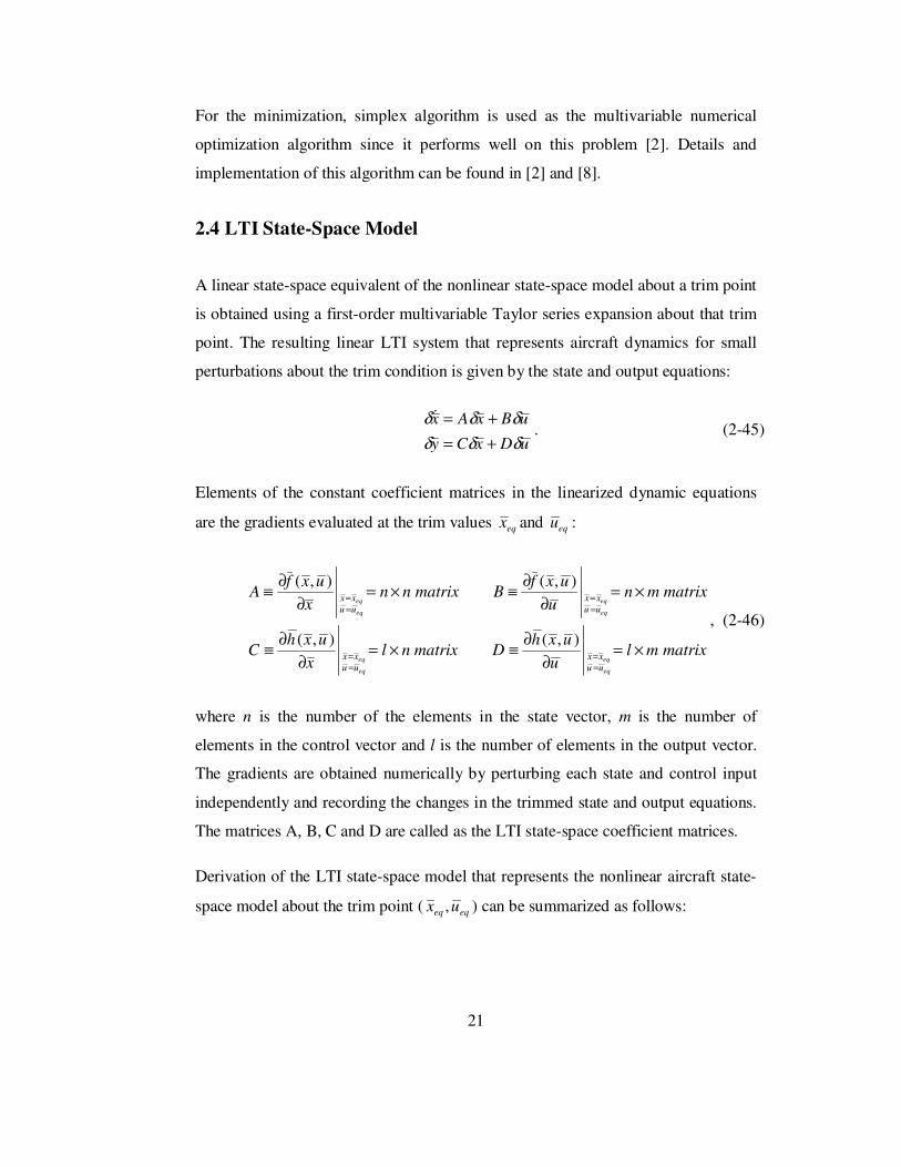
2.4 LTI State-Space Model

A linear state-space equivalent of the nonlinear state-space model about a trim point

is obtained using a first-order multivariable Taylor series expansion about that trim

point. The resulting linear LTI system that represents aircraft dynamics for small

perturbations about the trim condition is given by the state and output equations:

uDxCy

uBxAx

δδδ

δδδ

+=

+=&. (2-45)

Elements of the constant coefficient matrices in the linearized dynamic equations

are the gradients evaluated at the trim values eqx and equ :

matrixmlu

uxhDmatrixnl

x

uxhC

matrixmnu

uxfBmatrixnn

x

uxfA

eq

eq

eq

eq

eq

eq

eq

eq

uu

xx

uu

xx

uu

xx

uu

xx

×=∂

∂≡×=

∂

∂≡

×=∂

∂≡×=

∂

∂≡

==

==

==

==

),(),(

),(),(

, (2-46)

where n is the number of the elements in the state vector, m is the number of

elements in the control vector and l is the number of elements in the output vector.

The gradients are obtained numerically by perturbing each state and control input

independently and recording the changes in the trimmed state and output equations.

The matrices A, B, C and D are called as the LTI state-space coefficient matrices.

Derivation of the LTI state-space model that represents the nonlinear aircraft state-

space model about the trim point ( eqeq ux , ) can be summarized as follows:

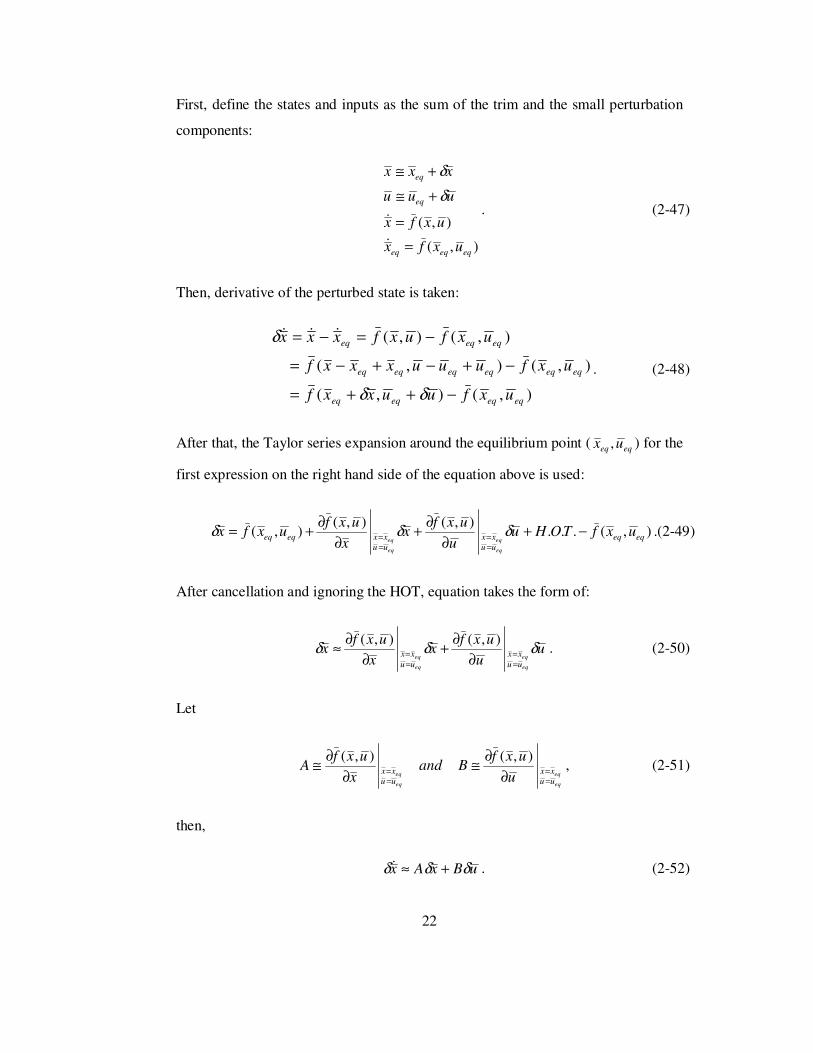
22

First, define the states and inputs as the sum of the trim and the small perturbation

components:

),(

),(

eqeqeq

eq

eq

uxfx

uxfx

uuu

xxx

=

=

+≅

+≅

&

&

δ

δ

. (2-47)

Then, derivative of the perturbed state is taken:

),(),(

),(),(

),(),(

eqeqeqeq

eqeqeqeqeqeq

eqeqeq

uxfuuxxf

uxfuuuxxxf

uxfuxfxxx

−++=

−+−+−=

−=−=

δδ

δ &&&

. (2-48)

After that, the Taylor series expansion around the equilibrium point ( eqeq ux , ) for the

first expression on the right hand side of the equation above is used:

),(...),(),(

),( eqeq

uu

xx

uu

xxeqeq uxfTOHuu

uxfx

x

uxfuxfx

eq

eq

eq

eq−+

∂

∂+

∂

∂+=

==

== δδδ .(2-49)

After cancellation and ignoring the HOT, equation takes the form of:

uu

uxfx

x

uxfx

eq

eq

eq

eq

uu

xx

uu

xx δδδ==

==

∂

∂+

∂

∂≈

),(),(. (2-50)

Let

eq

eq

eq

eq

uu

xx

uu

xxu

uxfBand

x

uxfA

==

==

∂

∂≅

∂

∂≅

),(),(, (2-51)

then,

uBxAx δδδ +≈& . (2-52)

23

Similarly, C and D matrices can be found by applying the Taylor series expansion

to the vector function h about the same trim point.

Hence, the following LTI model is obtained if only the states variables are used as

outputs, since C matrix turns out to be the identity matrix and D matrix is of no use:

xy

uBxAx

δδ

δδδ

=

+≈&. (2-53)

A useful subroutine to calculate the A, B, C and D matrices can be found in [2] and

[8]. If the EOM of the aircraft are implemented in Matlab/Simulink, an alternative

way to find the trim points and the linearized model of the aircraft is to use built-in

functions “trim” and “linmod” that are available in Matlab/Simulink [11], [9] and

[12]. Here, the former method given in [2] is used to find the matrices A and B.

2.5 Decoupling of the State-Space Models

Decoupling refers to the separation of EOMs into two independent sets. One set

describes longitudinal motion (pitching, and translation in the x-z plane) and the

other set describes lateral-directional motion (rolling, and side-slipping and yawing)

of the aircraft. In analytical studies, decoupled equations are very much easier to

work with. Decoupling occurs in both nonlinear and LTI state-space equations.

Here, only the decoupling of the LTI state-space equations just after the trim and

the linearization processes is used. If the entries of the LTI state-space coefficient

matrices that represent the relation of lateral state/input variables with longitudinal

state/input variables are small enough to be neglected, then the longitudinal and the

lateral-directional equations are decoupled (see Remark-2 below). So, the

longitudinal states and controls are:

[ ]

[ ]Tethlong

T

Tlong

u

powqhVx

δδ

θα

=

=, (2-54)

24

and the lateral-directional states and controls are:

[ ]

[ ]Tralat

T

lat

u

rpx

δδ

ψφβ

=

=. (2-55)

Remark-1: Although the LTI state-space models given above represent an aircraft

dynamics for small perturbations about a trim condition, the symbol “δ ” is not

used in front of the state and control variables from now on. Since, the LTI models

are used for the design purposes of the aircraft flight control systems, the symbol

“δ ” representing the small signal value of a state or a control variable is discarded.

Also, throughout the aircraft autopilot design processes, the word “lateral” is used

instead of the expression “lateral-directional”.

Remark-2: An example of the coupling between the lateral-directional and

longitudinal motions are represented with the orange colored entries of the system

matrix that are shown in Table 2-1. Here, the state and the control variables of the

coupled LTI model that is obtained by equation (2-53) are given as follows:

[ ][ ]raeth

T

T

u

rppowqhVx

δδδδ

ψφβθα

=

=. (2-56)

Table 2-1: System matrix, A, for the trim point given in Figure 4-3

-0.019 0 57.710 -31.694 -0.353 0.382 0 0 0 0 0

0 0 -565.601 565.601 0 0 0 0 0 0 0

0 0 -1.253 0 0.914 0 0 0 0 0 0

0 0 0 0 1.000 0 0 0 0 0 0

0 0 -2.032 0 -1.436 0 0 0 0 -0.003 0

0 0 0 0 0 -1.000 0 0 0 0 0

0 0 0 0 0 0 -0.320 0.055 0.029 -0.993 0

0 0 0 0 0 0 0 0 1.000 0.029 0

0 0 0 0 0.0003 0 -26.330 0 -3.838 0.649 0

0 0 0 0 0.003 0 11.844 0 -0.017 -0.517 0

0 0 0 0 0 0 0 0 0 1.000 0

25

Note that, after decoupling, the upper left 6-by-6 matrix shown with the yellow

color in Table 2-1 is the longitudinal system matrix, and the lower right 5-by-5

matrix shown with turquoise color is the lateral-directional system matrix.

It is obvious that there is a coupling between roll rate (p) and pitch rate (q), and also

between yaw rate (r) and pitch rate (q). However, these couplings can be neglected

since magnitudes of the entries (orange colored) of the system matrix that represent

the coupled variables are small enough. On the other hand, there is no coupling

between LTI models for the input matrix (see Table 2-2).

Table 2-2: Input matrix, B, for the trim point given in Figure 4-3

0 0.219 0 0

0 0 0 0

0 -0.002 0 0

0 0 0 0

0 -0.217 0 0

33.792 0 0 0

0 0 0 0.001

0 0 0 0

0 0 -0.870 0.157

0 0 -0.039 -0.076

0 0 0 0

Although this example illustrates the decoupling of the lateral-directional and

longitudinal LTI models found for the trim point # 5 (see Figure 4-3), similar

assumption is also applicable for the rest of the 11 trim points.

2.6 Flight Simulation

In order to simulate the flight of the aircraft to have an idea about how the state

trajectory (i.e. the position and the orientation of the aircraft in 3-D) evolves, a

numerical integration method is used. Both the linear and the nonlinear state-space

26

equations that are in the form of an initial value problem can be solved with a

numerical integration method. As mentioned before, initial values of the states and

controls can be found by the trimming process.

The state trajectory of the aircraft model changes continuously since the model

belongs to a physical system and the stored energy of this system is described by

the state variables. However, the numerical solution to the initial value problem by

the numerical integration method implies calculating discrete sequential values of

the state trajectory. Discrete time instants can be chosen based on either fixed time

step or variable time step. If the fixed time step is not specified properly by

considering stiffness of the equations, then the solution may not converge or error

made by the approximation method of the algorithm is magnified.

By considering spread of time constants in the system that models the aircraft, the

flight simulations are done based on an appropriate fixed time step by using Runge-

Kutta method (“Runge’s fourth-order rule”) as the numerical integration algorithm.

Details of this algorithm can be found in [2] and also in Matlab/Simulink

documentation [12].

27

CHAPTER 3

FLIGHT DYNAMICS OF A MISSILE

3.1 Introduction

Derivation of flight dynamics of a missile is similar to the derivation of an aircraft’s

flight dynamics. Important differences stem from the symmetry axes of the vehicle.

In the first part of this chapter, assumptions and the important points to derive the

flight dynamics of a canard controlled, skid-to-turn type missile that are formulated

in [13] are summarized. Since a detailed derivation of flight dynamics of an aircraft

has been given in Chapter 2, only the resultant LTI state-space models obtained

after trimming, linearization and decoupling processes are given here.

In the second part of the chapter, based on the LTI state-space models derived in

[13], missile flight control system design details are explained.

It is important to note that, the same coordinate systems defined for the aircraft are

also applicable for the missile. In addition, Assumption 1, Assumption 2,

Assumption 6 and

Assumption 7 holds for the missile, whereas Assumption 4 and Assumption 5 are

not applicable. Besides, Assumption 3 is modified such that the missile has three

symmetry axes that coincide with its body axes, so 0=== yzxzxy III . Also, due to

28

the symmetry of the missile used in this study, zy II = . As a result, inertia matrix is

simplified with these equations.

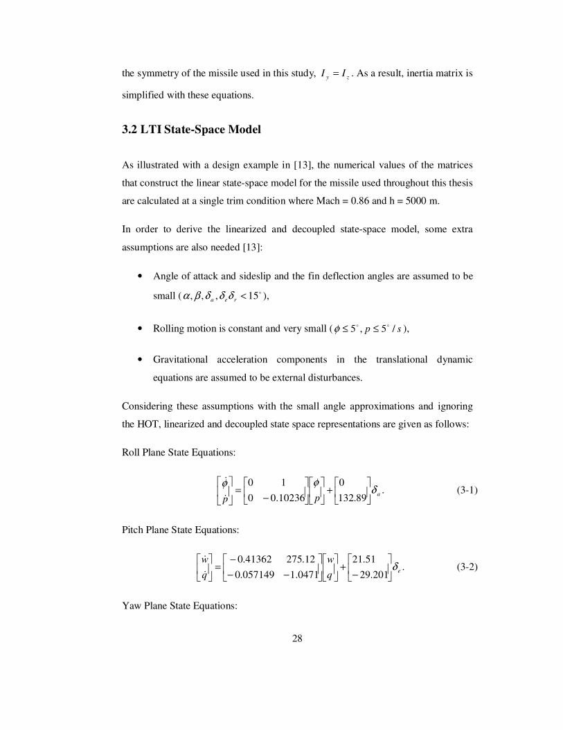
3.2 LTI State-Space Model

As illustrated with a design example in [13], the numerical values of the matrices

that construct the linear state-space model for the missile used throughout this thesis

are calculated at a single trim condition where Mach = 0.86 and h = 5000 m.

In order to derive the linearized and decoupled state-space model, some extra

assumptions are also needed [13]:

• Angle of attack and sideslip and the fin deflection angles are assumed to be

small ( o15,,, <rea δδδβα ),

• Rolling motion is constant and very small ( sp /5,5 oo ≤≤φ ),

• Gravitational acceleration components in the translational dynamic

equations are assumed to be external disturbances.

Considering these assumptions with the small angle approximations and ignoring

the HOT, linearized and decoupled state space representations are given as follows:

Roll Plane State Equations:

app

δφφ

+

−=

89.132

0

10236.00

10

&

&

. (3-1)

Pitch Plane State Equations:

eq

w

q

wδ

−+

−−

−=

201.29

51.21

0471.1057149.0

12.27541362.0

&

&. (3-2)

Yaw Plane State Equations:

29

rr

v

r

vδ

+

−

−−=

201.29

51.21

0471.1057149.0

12.27541362.0

&

&. (3-3)

Remark: Although the LTI state-space models given above represent missile

dynamics for small perturbations about the trim condition, the symbol “δ ” is not

used in front of the state and control variables of the missile. However, that symbol

is used to discriminate the state and control variables of the LTI and the nonlinear

state-space models of aircraft. Since, only the LTI models are used for the design

purposes of missile flight control systems and missile guidance systems, the symbol

“δ ” is discarded.

Normally, there are 12 nonlinear state equations that model the dynamics of the

missile. The linear equations given at (3-1), (3-2) and (3-3) represent 6 of the

nonlinear state equations. The rest of them considering the assumptions and the

linearization process are given as follows:

ψψθ

θψ

θ

θθ

ψθψψθ

sincoscos

.cos

cossin

sinsincossincos

vux

constu

r

q

wuz

wvuy

−=

=

=

=

+−=

++=

&

&

&

&

&

. (3-4)

Note that, equations (3-1), (3-2), (3-3) and (3-4) are used in flight simulations to get

the state trajectory of the missile.

30

CHAPTER 4

AUTOPILOT OF THE AIRCRAFT

4.1 Introduction

Autopilot of an aircraft can be designed via classical or modern control techniques.

The former requires closure of one-loop-at-a-time by such tools as root locus, Bode

and Nyquist plots and so on, whereas by using the latter, all the control gains are

calculated simultaneously and hence all the loops are closed at once.

Generally, a classical control technique such as PID necessitates the tuning of its

parameters for each control loop by trial-and-error. Although Ziegler-Nichols

tuning of a PID compensator works for a large class of industrial systems, the

design procedure becomes more complex as more loops are existing. As a result,

often PID technique is not preferred for controlling MIMO systems. However, a

modern control technique such as LQR is fundamentally a time-domain design

technique useful in shaping the closed-loop response in contrast to the classical

controls, where most techniques are in the frequency domain [2]. By using LQR,

one can design a controller for a MIMO system satisfying the performance

specifications like rise time, overshoot and settling time, by selecting the precise

performance criterion. As a consequence, this technique is mostly used in the design

of stability augmentation systems and autopilots.

31

For the design of lateral and longitudinal aircraft autopilots, both LQR and PID

techniques are used in this study. Tuning of the PID parameters are done via an

optimization technique choosing a suitable cost function to satisfy the closed loop

stability and the performance specifications.

Finally, it is important to note that, both of the controller design techniques are

applied on lateral and longitudinal LTI state-space models derived in section 2.5 for

each of 12 trim points that are chosen in the flight envelope of the aircraft. Then, the

resultant lateral and longitudinal controllers are used on the nonlinear aircraft model

by gain scheduling depending on the speed and the altitude of the aircraft. Note that

the local controller gains found for each trim point are linearly interpolated within

the flight envelope to find the global controller gains.

4.2 Linear Quadratic Controller (LQC) Design

4.2.1 Linear Quadratic Regulator (LQR)

The LQR is an optimal control method used on a linear system so that the states of

this linear system are regulated to zero by minimizing a quadratic cost function as

follows:

( )dttuRtutxQtxtutxJTT

∫∞

+=0

)()()()(2

1))(),(( , (4-1)

where, nRx ∈ is the state vector, r

Ru ∈ is the control vector, and nnRQ

×∈ is a

positive semi-definite matrix, rrRR

×∈ is a positive definite matrix and J is the

performance index.

By minimizing the performance index with the selection of suitable Q and R, a

feedback gain “K” can be found such that the control is optimal in order to satisfy

the time-domain performance criteria, such as settling time, overshoot and rise time.

32

)()( txKtu −= . (4-2)

If all of the states are available, then an LQR with full-state feedback design is used,

as in our case throughout this thesis. But if all the states are not available, then an

LQR with output feedback design is used. The output feedback design is not in the

scope of this study. More information about these techniques can be found in [2]

and [1].

For a linear system described by:

)()(

)()()(

txty

tuBtxAtx

=

+=&, (4-3)

controllability of the pair ( )BA, and observability of the pair ( )AH , guarantee the

closed loop stability of this LQR with state feedback [2]. Here, H is any matrix such

that HHQT= .

Substituting (3-2) into (3-3) results in the following closed loop system:

)()(

)()()()(

txty

txAtxBKAtx C

=

=−=&. (4-4)

In fact, finding the Q and R matrices requires trial-and-error, so, engineering comes

into play to find suitable values for them. The next section briefly describes how to

select these parameters.

For a selected (Q,R) pair, the feedback gain K is found by solving the LQR problem

via the function “lqr” in Matlab. By using “lqr”, the closed loop stability of the

system is obtained, since the controllability of the pair ( )BA, and the observability

of the pair ( )AH , are checked as an initial step. More details on the analytical

solution to the problem can be found in [17], [2], [18] and [10].

33

4.2.2 Selection of Quadratic Weights: Q and R

The selection of Q and R necessitates the engineering judgment. In different

designs, they may be selected for different performance requirements. If they are

both chosen nonsingular, then all of the state vector )(tx and control vector )(tu

will eventually go to zero if J has a finite value. Since the minimization of J is a

type of minimum energy problem, the aim of this optimal control method, LQR, is

to minimize the energy in the states without using too much control energy [2].

The relative magnitudes of Q and R determine smallness of the states relative to

those of the controls. For example, a larger R penalizes the controls more so that the

state vector will be in greater norm relative to the control vector. On the other hand,

Q is chosen larger in order to make the states go to zero quickly.

It is worth noting that the selection of Q and R determines the closed-loop pole

positions which, in fact, shape the time response of the closed-loop system.

4.2.3 Suboptimal Linear Quadratic Tracker (SLQT)

Flight control systems generally require the direct application of the LQR for the

inner control loops that determine the stability of the system. These inner loops are

the rate loops. However, the controller specifications may require not always the

regulation of the states to zero, but also some of them may be wanted to track a

nonzero reference command signal, r(t). This type of a problem is called as servo

design problem and it has many implementations in the design of control

augmentation systems that contain stability augmentation systems as inner loops.

The optimal linear quadratic tracker is not a causal system. It depends on solving an

adjoint system of differential equations backward in time, and so is impossible to be

implemented. Instead, a suboptimal “steady-state” tracker is used [2]. Then, the

design problem turns out to be a suboptimal linear quadratic tracker problem with

the following cost function (or performance index):

34

( ) ( )∫∞

+=0

)()()()(2

1)(),( dttuRtuteQtetuteJ

TT , (4-5)

where, the tracking error and the performance output are formulated respectively as:

)()()( tytrte −= , (4-6)

)()( txCty = . (4-7)

The sub-optimality stems from the fact that, the performance index does not

necessarily minimize a quadratic function of the total tracking error [2].

Solution to the steady-state tracker problem is similar to the one defined previously

for the LQR. Depending on the type of the LTI system on which the SLQT is

applied, one of the two different techniques is used as explained in the preceding

sections.

4.2.3.1 SLQT Design for Type 0 LTI System

An SLQT for an LTI system that has no integrator, that is to say type 0, can be

constructed as follows [1]:

Figure 4-1: Servomechanism for a type 0 LTI system [1].

35

Here, the control signal u, the output signal y and the reference step signal r are

scalars, and nnnnnRKRCRBRA

×××× ∈∈∈∈ 111 ,,, . From the diagram above,

following equations are obtained:

BuxAx +=& , (4-8)

xCy = , (4-9)

ξIkxKu +−= , (4-10)

xCryr −=−=ξ& . (4-11)

The pair (A, B) is assumed to be controllable and also BAsIC1)( −− is assumed to

have no zero at the origin to avoid the pole zero cancellation due to the integrator

inserted in the feed-forward path. Suppose that the reference step input is applied at

0=t . Then, by combining the equations (4-8) and (4-11) for 0>t , the system

dynamics takes the form:

)(1

0)(

0)(

)(

0

0

)(

)(trtu

B

t

tx

C

A

t

tx

+

+

−=

ξξ&

&. (4-12)

At steady state, (4-12) turns into:

)(1

0)(

0)(

)(

0

0

)(

)(∞

+∞

+

∞

∞

−=

∞

∞ru

Bx

C

Ax

ξξ&

&. (4-13)

An asymptotically stable system can be designed such that )(),( ∞∞ ux and )(∞ξ

converge to constant values and hence, 0)( =∞ξ& and ry =∞)( .

By defining:

)()()(

)()()(

)()()(

∞−=

∞−=

∞−=

ututu

tt

xtxtx

e

e

e

ξξξ , (4-14)

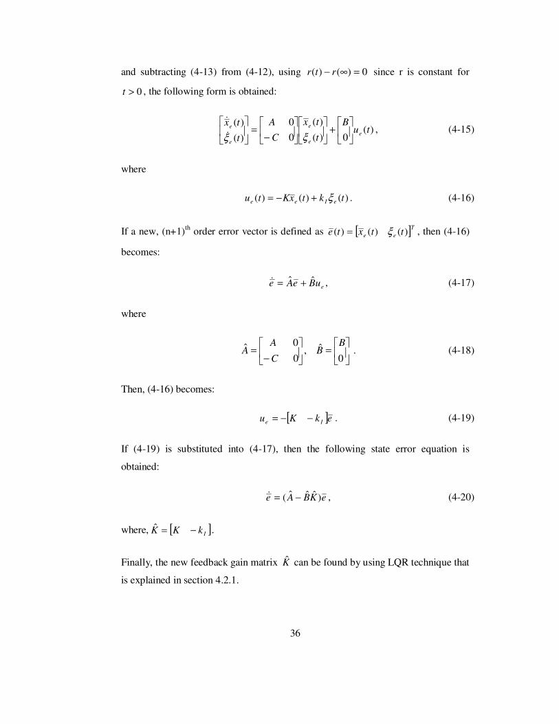
36

and subtracting (4-13) from (4-12), using 0)()( =∞− rtr since r is constant for

0>t , the following form is obtained:

)(0)(

)(

0

0

)(

)(tu

B

t

tx

C

A

t

txe

e

e

e

e

+

−=

ξξ&

&, (4-15)

where

)()()( tktxKtu eIee ξ+−= . (4-16)

If a new, (n+1)th order error vector is defined as [ ]T

ee ttxte )()()( ξ= , then (4-16)

becomes:

euBeAe ˆˆ +=& , (4-17)

where

=

−=

0ˆ,

0

0ˆ BB

C

AA . (4-18)

Then, (4-16) becomes:

[ ]ekKu Ie −−= . (4-19)

If (4-19) is substituted into (4-17), then the following state error equation is

obtained:

eKBAe )ˆˆˆ( −=& , (4-20)

where, [ ]IkKK −=ˆ .

Finally, the new feedback gain matrix K̂ can be found by using LQR technique that

is explained in section 4.2.1.

37

4.2.3.2 SLQT Design for Type 1 LTI System

If the LTI system defined by (4-8) has an integrator, then there is no need to add an

integrator to the feed-forward path shown in Figure 4-1, so the resultant block

diagram of the controller is as follows:

Figure 4-2: Servomechanism for a type 1 LTI system [1].

According to the state-feedback control scheme shown above,

rkxKu I+−= , (4-21)

where, K is the feedback gain matrix defined by [ ]nkkkK L21= . Then, the

state dynamics can be described by:

rBkxBKABuxAtx I+−=+= )()(& . (4-22)

After defining )()()( ∞−= xtxte and using the similar steps used in the previous

section, the error dynamics can be described by:

38

eBKAe )( −=& . (4-23)

Hence, the feedback gain matrix K can be found by using LQR technique that is

explained in section 4.2.1.

4.2.4 Gain Scheduling

The trimming process explained in section 2.3 is used to obtain the trim points in

flight envelope of the aircraft. Borders of the flight envelope are given roughly in

Appendix A.1. In order to see the trimming performance at the trim points, the trim

values of the state and control variables are used as initial conditions for the

nonlinear model and tested with zero input to check if the linear and angular

accelerations are close to zero. Also, maximum value of the cost function of the

trim process which is given in equation (2-43) is checked if it is close to zero.

In order to design the lateral and longitudinal autopilots of the aircraft by using

LQC technique, 12 trim points shown in the Figure 4-3 are used:

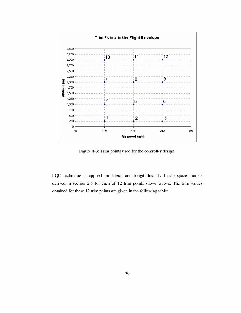
39

Figure 4-3: Trim points used for the controller design.

LQC technique is applied on lateral and longitudinal LTI state-space models

derived in section 2.5 for each of 12 trim points shown above. The trim values

obtained for these 12 trim points are given in the following table:

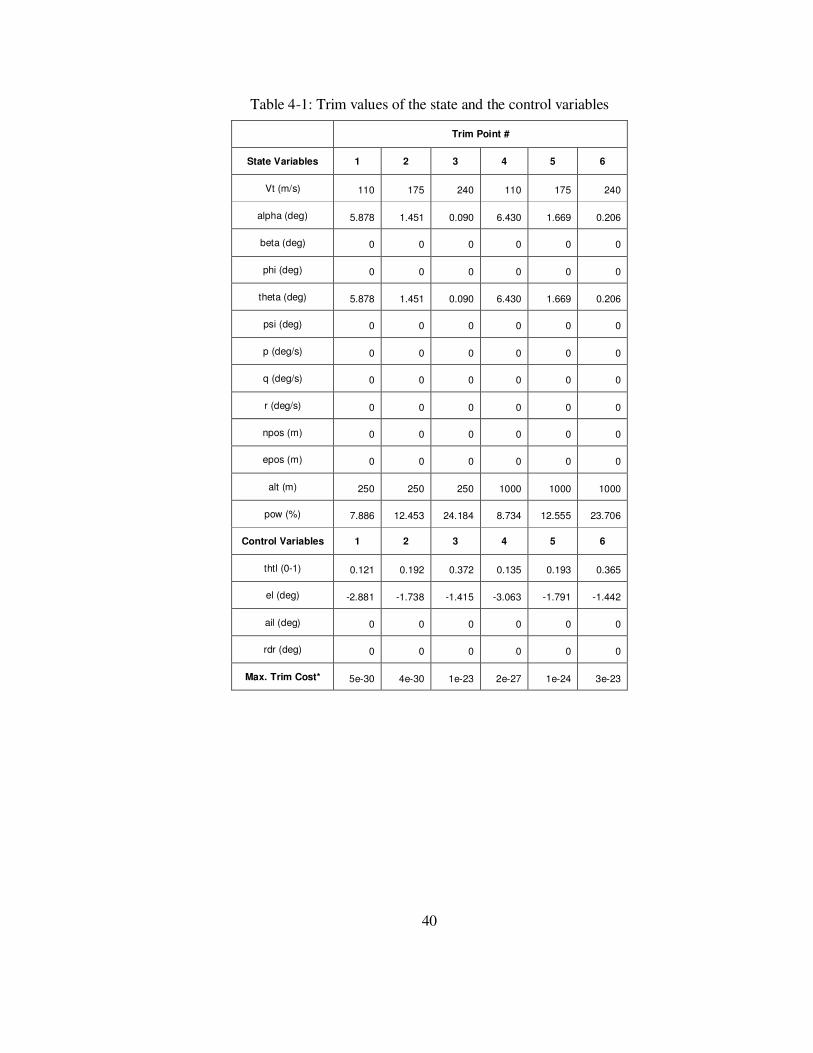
40

Table 4-1: Trim values of the state and the control variables

Trim Point #

State Variables 1 2 3 4 5 6

Vt (m/s) 110 175 240 110 175 240

alpha (deg) 5.878 1.451 0.090 6.430 1.669 0.206

beta (deg) 0 0 0 0 0 0

phi (deg) 0 0 0 0 0 0

theta (deg) 5.878 1.451 0.090 6.430 1.669 0.206

psi (deg) 0 0 0 0 0 0

p (deg/s) 0 0 0 0 0 0

q (deg/s) 0 0 0 0 0 0

r (deg/s) 0 0 0 0 0 0

npos (m) 0 0 0 0 0 0

epos (m) 0 0 0 0 0 0

alt (m) 250 250 250 1000 1000 1000

pow (%) 7.886 12.453 24.184 8.734 12.555 23.706

Control Variables 1 2 3 4 5 6

thtl (0-1) 0.121 0.192 0.372 0.135 0.193 0.365

el (deg) -2.881 -1.738 -1.415 -3.063 -1.791 -1.442

ail (deg) 0 0 0 0 0 0

rdr (deg) 0 0 0 0 0 0

Max. Trim Cost* 5e-30 4e-30 1e-23 2e-27 1e-24 3e-23

41

Table 4-2: Trim values of the state and the control variables – cont’d

Trim Point #

State Variables 7 8 9 10 11 12

Vt (m/s) 110 175 240 110 175 240

alpha (deg) 7.245 1.994 0.379 8.162 2.361 0.575

beta (deg) 0 0 0 0 0 0

phi (deg) 0 0 0 0 0 0

theta (deg) 7.245 1.994 0.379 8.162 2.361 0.575

psi (deg) 0 0 0 0 0 0

p (deg/s) 0 0 0 0 0 0

q (deg/s) 0 0 0 0 0 0

r (deg/s) 0 0 0 0 0 0

npos (m) 0 0 0 0 0 0

epos (m) 0 0 0 0 0 0

alt (m) 2000 2000 2000 3000 3000 3000

pow (%) 10.269 12.819 23.103 12.430 13.274 22.540

Control Variables 7 8 9 10 11 12

thtl (0-1) 0.158 0.197 0.356 0.191 0.204 0.347

el (deg) -3.332 -1.868 -1.484 -3.633 -1.956 -1.530

ail (deg) 0 0 0 0 0 0

rdr (deg) 0 0 0 0 0 0

Max. Trim Cost* 1e-29 6e-29 3e-25 1e-29 4e-30 3e-25

*: This value is obtained after testing of the trim values on the nonlinear aircraft

model within 100 seconds.

The resultant lateral and longitudinal controller gains are scheduled with respect to

the airspeed and the altitude, and the controllers are applied on the nonlinear aircraft

model to check the design performance as shown below:

42

Figure 4-4: Block diagram used to test the performance of the autopilot designed for

an LTI system at a single trim point

The controller gains for the points in the flight envelope that do not correspond to

the trim points, are calculated by using the linear interpolation method. Built-in

interpolation algorithm of Simulink is used for this purpose.

4.2.5 Gain Scheduled LQC Design

4.2.5.1 Longitudinal LQC Design

The LTI longitudinal system for the aircraft is composed of the states and controls

defined in (2-54). For the 12 trim points given in the previous section, controller

structure formulated in section 4.2.3.1 is used to design the longitudinal flight

43

control system of the aircraft. The following figure illustrates the block diagrams

used for the design process.

Figure 4-5: Longitudinal autopilot of the aircraft designed with SLQT

Table 4-3 shows the selection of Q and R matrices for the longitudinal LQC design.

These values are determined by trial and error. It is important to note that, the

closed loop stability is satisfied even if the reference signal magnitudes given in the

next table are applied to the nonlinear (NL) system.

Note that, the reason of choosing some of the delta speed reference signal

amplitudes smaller than the others (in Table 4-4) is the maximum speed constraint

(which is 270 m/s) for the flight envelope. Also, note that the diagonal entries of the

diagonal Q and R matrices are shown as they are represented in Matlab in order to

save space.

44

Table 4-3: Selection of Q and R for the longitudinal LQC design

Trim Point # Weighting Matrices

Values

Q diag(1, 1, 1, 1, 1, 1, 2000, 20) 1

R diag(300000000, 150000)

Q diag(1, 1, 1, 1, 1, 1, 300, 1) 2

R diag(25000000, 10000)

Q diag(1, 1, 1, 1, 1, 1, 1500, 1) 3

R diag(10000000, 30000)

Q diag(1, 1, 1, 1, 1, 1, 2000, 20) 4

R diag(500000000, 3000000)

Q diag(1, 1, 1, 1, 1, 1, 300, 1) 5

R diag(30000000, 50000)

Q diag(1, 1, 1, 1, 1, 1, 2000, 1) 6

R diag(10000000, 80000)

Q diag(1, 1, 1, 1, 1, 1, 20, 1) 7

R diag(10000000, 1000000)

Q diag(1, 1, 1, 1, 1, 1, 100, 1) 8

R diag(50000000, 500000)

Q diag(1, 1, 1, 1, 1, 1, 2000, 1) 9

R diag(20000000, 80000)

Q diag(1, 1, 1, 1, 1, 1, 50, 1) 10

R diag(20000000, 1000000)

Q diag(1, 1, 1, 1, 1, 1, 200, 1) 11

R diag(50000000, 200000)

Q diag(1, 1, 1, 1, 1, 1, 1000, 1) 12

R diag(50000000, 100000)

Table 4-4: Longitudinal LQC design

Max. Reference Step Commands Trim Point #

delta_V (m/s) delta_h (m)

1 65 750

2 65 750

3 30 750

4 65 1000

5 65 1000

6 30 1000

7 65 1000

8 65 1000

9 30 1000

10 65 1000

11 65 1000

12 30 1000

45

4.2.5.2 Lateral LQC Design

The LTI lateral system for the aircraft is composed of the states and controls

defined in (2-55). For the 12 trim points, the controller structure formulated in

section 4.2.3.2 is used to design the lateral flight control system. The following

figure illustrates the block diagrams used for the design process:

Figure 4-6: Lateral autopilot of the aircraft designed with SLQT

Table 4-5 shows the selection of Q and R matrices for the lateral LQC design.

These values are determined by trial and error. It is important to note that, the

closed loop stability is satisfied even if the reference signal magnitudes given in the

next table are applied to the nonlinear (NL) system.

46

Table 4-5: Selection of Q and R for the lateral LQC design

Trim Point # Weighting Matrices

Values

Q diag(1, 1, 1, 1, 1000) 1

R diag(100000, 8)

Q diag(1, 1, 1, 1, 2000) 2

R diag(5000000, 5)

Q diag(1, 1, 1, 1, 10) 3

R diag(200, 1)

Q diag(1, 1, 1, 1, 1000) 4

R diag(100000, 10)

Q diag(1, 1, 1, 1, 5000) 5

R diag(10000000, 30)

Q diag(1, 1, 1, 1, 10) 6

R diag(150, 1)

Q diag(1, 1, 1, 1, 400) 7

R diag(100000, 30)

Q diag(1, 1, 1, 1, 2000) 8

R diag(10000000, 10)

Q diag(1, 1, 1, 1, 10) 9

R diag(100, 7)

Q diag(1, 1, 1, 1, 600) 10

R diag(100000, 40)

Q diag(1, 1, 1, 1, 1000) 11

R diag(5000000, 10)

Q diag(1, 1, 1, 1, 30) 12

R diag(500, 1)

Table 4-6: Lateral LQC design

Max. Reference Step Command

delta_yaw (deg) Trim Point #1 to #12

179

47

4.2.6 Gain Scheduled LQC Design Performance

The resultant lateral and longitudinal autopilots designed by gain scheduled LQC

method are combined and then tested by applying reference signals (i.e. delta speed,

delta height and delta yaw, simultaneously) to the nonlinear system. In order to

illustrate the performance of the resultant autopilot, the following case is given:

Test Case: The state and input trim values for the initial point at which V0=175 m/s

and h0=2000 m are found by the trimming algorithm given in section 2.3. Then,

delta speed, delta height and delta yaw step reference signals are applied

simultaneously; that is to say, the height and the speed of the aircraft are increased,

while making a coordinated turn in the horizontal plane. The step responses of the

gain scheduled autopilot are given with the following figures:

0 20 40 60 80 100-100

0

100

200

300

400

time(s)

delta h

eig

ht

(m)

Actual Height

Desired Height

Figure 4-7: Height response of the LQC from the point A to the point B

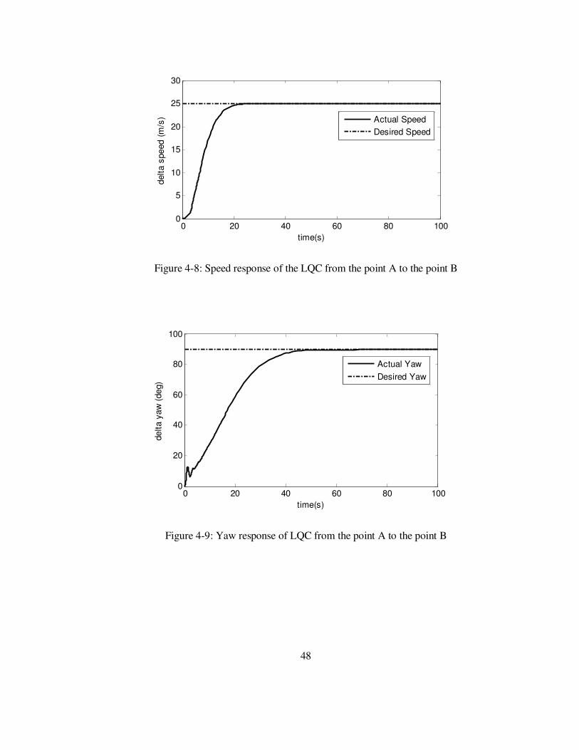
48

0 20 40 60 80 1000

5

10

15

20

25

30

time(s)

delta s

peed (

m/s

)

Actual Speed

Desired Speed

Figure 4-8: Speed response of the LQC from the point A to the point B

0 20 40 60 80 1000

20

40

60

80

100

time(s)

delta y

aw

(deg)

Actual Yaw

Desired Yaw

Figure 4-9: Yaw response of LQC from the point A to the point B

49

4.3 Proportional Integral Derivative (PID) Controller Design

For the longitudinal and lateral autopilots, the controller structures are given in

Figure 4-10 and Figure 4-11. In order to tune the proportional, integral and

derivative coefficients of each PID controller, the optimization algorithm “fmincon”

of the Matlab Optimization Toolbox is used. By defining necessary bounds for the

coefficients to be tuned and also a suitable cost function, the optimization algorithm

finds a solution that satisfies a user defined stopping criteria, for example, the

directional derivative, 1-D search step length, change in the cost function value or

change in the magnitude of the coefficient vector to be tuned.

Lateral and longitudinal autopilot structures used for the PID controller are shown

in the figures below.

Figure 4-10: Longitudinal autopilot of the aircraft designed with PID

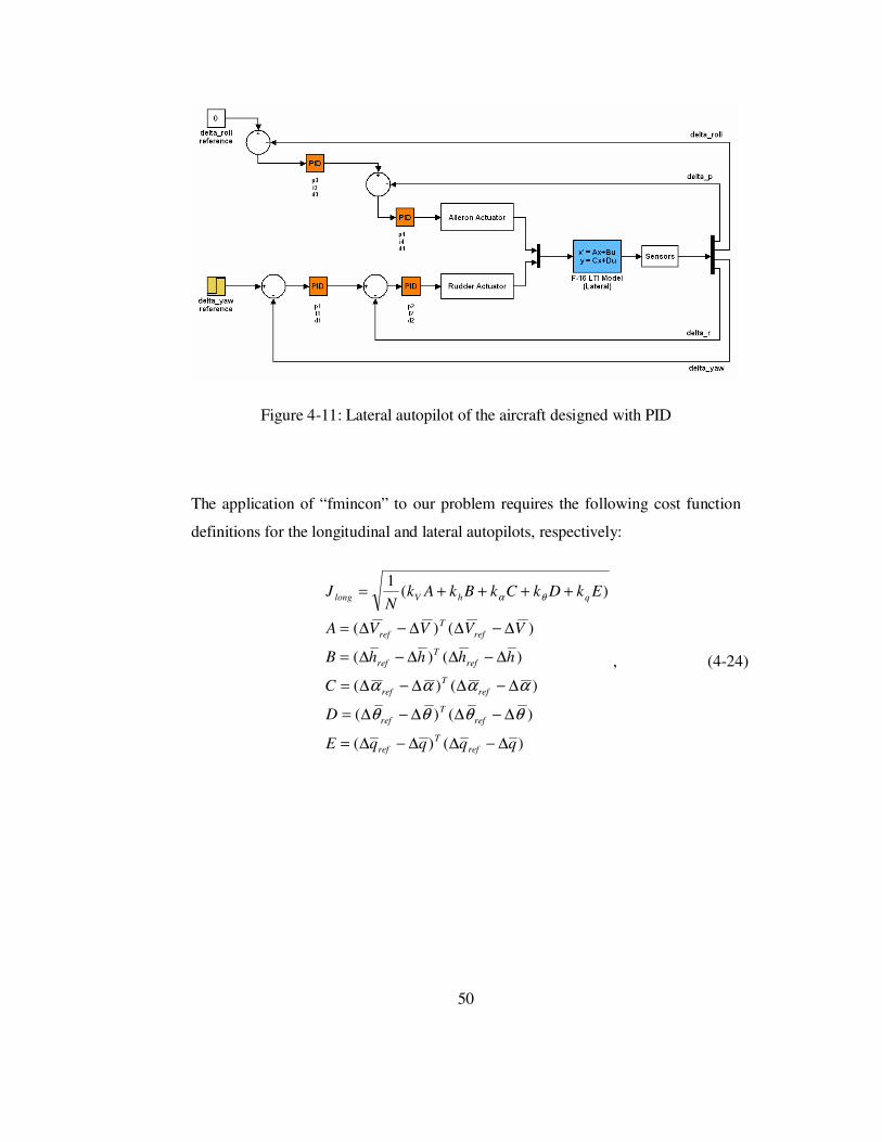
50

Figure 4-11: Lateral autopilot of the aircraft designed with PID

The application of “fmincon” to our problem requires the following cost function

definitions for the longitudinal and lateral autopilots, respectively:

)()(

)()(

)()(

)()(

)()(

)(1

qqqqE

D

C

hhhhB

VVVVA

EkDkCkBkAkN

J

ref

T

ref

ref

T

ref

ref

T

ref

ref

T

ref

ref

T

ref

qhVlong

∆−∆∆−∆=

∆−∆∆−∆=

∆−∆∆−∆=

∆−∆∆−∆=

∆−∆∆−∆=

++++=

θθθθ

αααα

θα

, (4-24)

51

)()(

)()(

)()(

)()(

)()(

)(1

ψψψψ

φφφφ

ββββ

ψφβ

∆−∆∆−∆=

∆−∆∆−∆=

∆−∆∆−∆=

∆−∆∆−∆=

∆−∆∆−∆=

++++=

ref

T

ref

ref

T

ref

ref

T

ref

ref

T

ref

ref

T

ref

rplat

E

rrrrD

ppppC

B

A

EkDkCkBkAkN

J

, (4-25)

where, N is the number of total time steps and the vector VVref ∆−∆ is an Nx1

vector that stores the delta speed error value for each time step.

Also note that, the reference values of the variables other than the controlled ones

are taken as zero for the applications given below. Only the weight values (k’s) of

the error for each state variable change as indicated for each of the application (see

the example below).

By choosing a suitable initial condition for the coefficients, the algorithm is run at

fixed step size for tfinal seconds for each iteration steps of the “fmincon”. Finally, the

solution is found for the user specified termination condition.

4.3.1 PID Controller Design Example

In order to illustrate the utilization of the optimization algorithm on our problem,

the state trim values and input trim values are used that are the solution of the trim

algorithm given in section 2.3 for the speed of 150 m/s and the altitude of 680 m,

(for the lateral and longitudinal autopilots of the following example).

4.3.1.1 Longitudinal Autopilot

The parameter selection for this design is given as follows:

52

[ ] [ ]1001010

01.0

100

1

/1

=

=∆

=

=∆

=∆

qhV

final

ref

ref

kkkkk

st

st

mh

smV

θα

. (4-26)

The optimization process is completed in 75 iterations after reaching the directional

derivative of 6e-8 and the final cost value is 0.438675. So, the final values of the

PID coefficients are given in the following table (note that, the first row

corresponds to the initial conditions):

p1 i1 d1 p2 i2 d2 p3 i3 d3 p4 i4 d4

0.003 0 0 1 0 0 -1 0 0 1 1 1

0.693 0.034 0.130 34.976 0 4.593 -0.203 -3.942 -0.106 13.861 0 16.036

0 20 40 60 80 100-0.2

0

0.2

0.4

0.6

0.8

1

1.2

time(s)

speed (

m/s

)

Desired

LTI Response

NL Response

Figure 4-12: Step response of the longitudinal autopilot for delta speed command

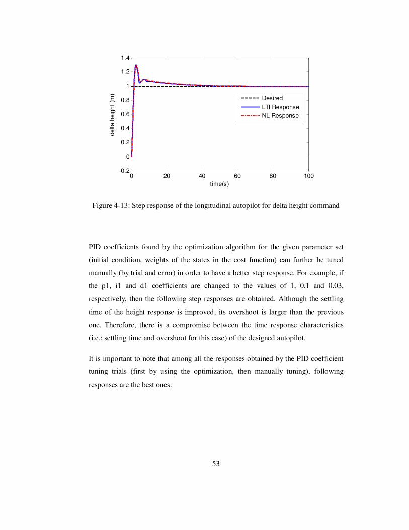
53

0 20 40 60 80 100-0.2

0

0.2

0.4

0.6

0.8

1

1.2

1.4

time(s)

delta h

eig

ht

(m)

Desired

LTI Response

NL Response

Figure 4-13: Step response of the longitudinal autopilot for delta height command

PID coefficients found by the optimization algorithm for the given parameter set

(initial condition, weights of the states in the cost function) can further be tuned

manually (by trial and error) in order to have a better step response. For example, if

the p1, i1 and d1 coefficients are changed to the values of 1, 0.1 and 0.03,

respectively, then the following step responses are obtained. Although the settling

time of the height response is improved, its overshoot is larger than the previous

one. Therefore, there is a compromise between the time response characteristics

(i.e.: settling time and overshoot for this case) of the designed autopilot.

It is important to note that among all the responses obtained by the PID coefficient

tuning trials (first by using the optimization, then manually tuning), following

responses are the best ones:

54

0 20 40 60 80 100-0.2

0

0.2

0.4

0.6

0.8

1

1.2

time(s)

delta s

peed (

m/s

)

Desired

LTI Response

NL Response

Figure 4-14: Step response of the longitudinal autopilot after manual tuning - 1

0 20 40 60 80 100-0.5

0

0.5

1

1.5

2

time(s)

delta h

eig

ht

(m)

Desired

LTI Response

NL Response

Figure 4-15: Step response of the longitudinal autopilot after manual tuning – 2

55

4.3.1.2 Lateral Autopilot

The parameter selection for this design is given as follows:

[ ] [ ]55511

01.0

100

1

=

=∆

=

=∆

ψφβ

ψ

kkkkk

st

st

rp

final

ref

o

. (4-27)

The optimization process is completed in 42 iterations after reaching the directional

derivative of -1e-9 and the final cost value is 0.256912. So, the final values of the

PID coefficients are given in the following table (note that, the first row

corresponds to the initial conditions):

p1 i1 d1 p2 i2 d2 p3 i3 d3 p4 i4 d4

1 0 0 -1 0 0 1 0 0 -1 0 0

5.514 0.004 4.061 -4.445 0 -0.350 0.318 0 0 -1.948 -0.002 -1.397

0 10 20 30 40 50 60 70 80 90 1000

0.2

0.4

0.6

0.8

1

1.2

1.4

time(s)

delta y

aw

(deg)

Desired

LTI Response

NL Response

Figure 4-16: Step response of the lateral autopilot for delta yaw command

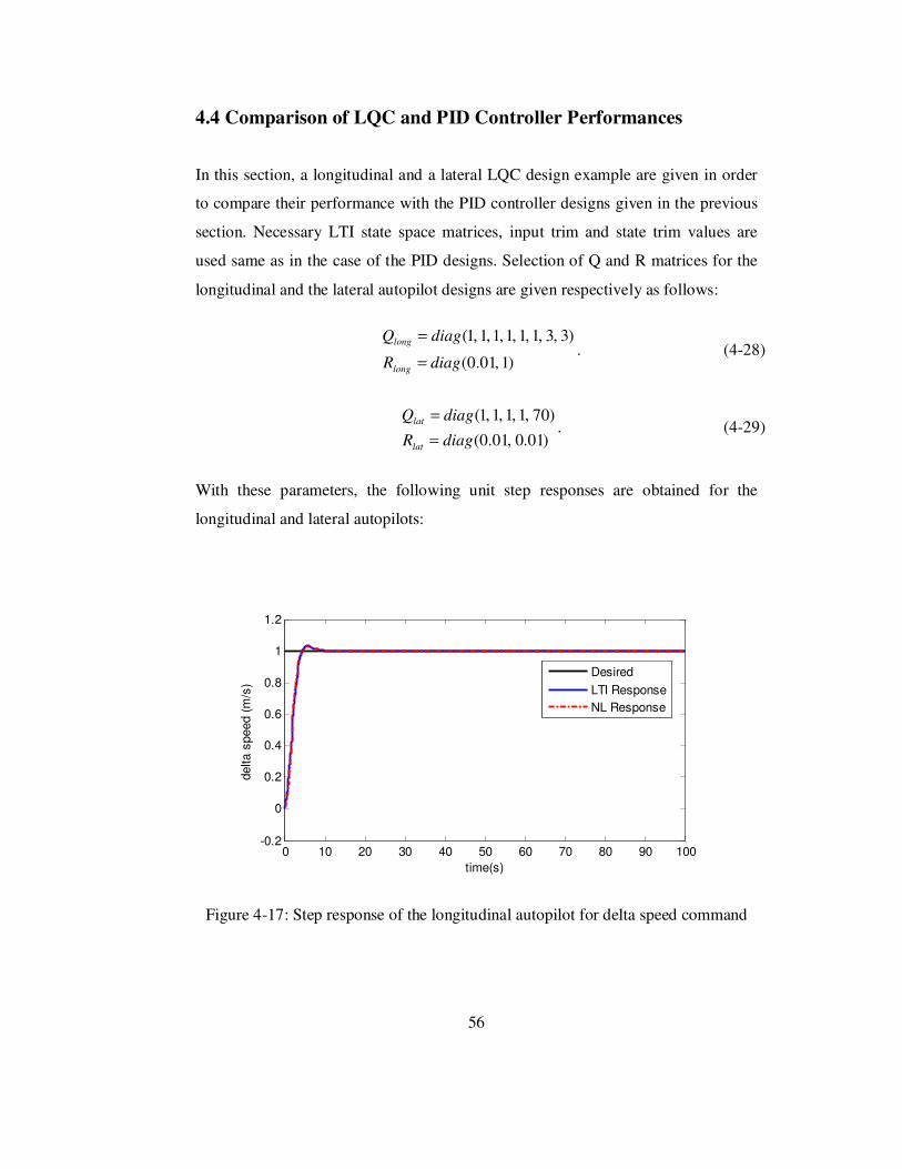
56

4.4 Comparison of LQC and PID Controller Performances

In this section, a longitudinal and a lateral LQC design example are given in order

to compare their performance with the PID controller designs given in the previous

section. Necessary LTI state space matrices, input trim and state trim values are

used same as in the case of the PID designs. Selection of Q and R matrices for the

longitudinal and the lateral autopilot designs are given respectively as follows:

)1,01.0(

)3,3,1,1,1,1,1,1(

diagR

diagQ

long

long

=

=. (4-28)

)01.0,01.0(

)70,1,1,1,1(

diagR

diagQ

lat

lat

=

=. (4-29)

With these parameters, the following unit step responses are obtained for the

longitudinal and lateral autopilots:

0 10 20 30 40 50 60 70 80 90 100-0.2

0

0.2

0.4

0.6

0.8

1

1.2

time(s)

delta s

peed (

m/s

)

Desired

LTI Response

NL Response

Figure 4-17: Step response of the longitudinal autopilot for delta speed command

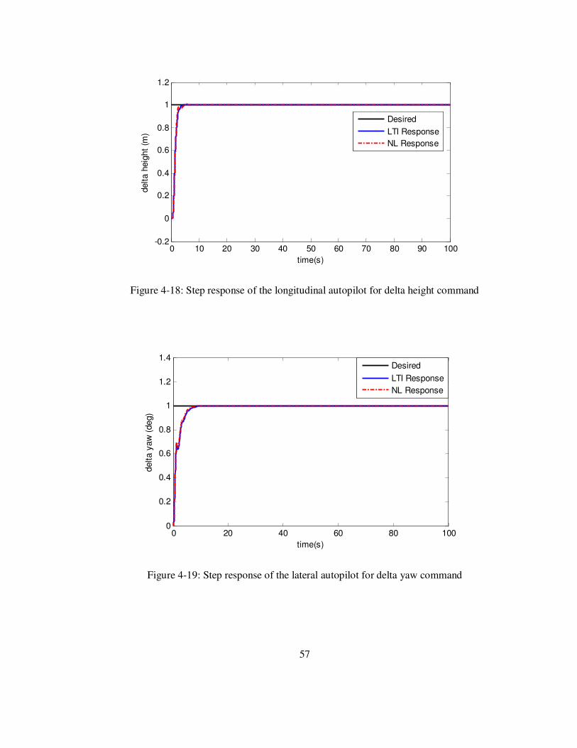
57

0 10 20 30 40 50 60 70 80 90 100-0.2

0

0.2

0.4

0.6

0.8

1

1.2

time(s)

delt

a h

eig

ht

(m)

Desired

LTI Response

NL Response

Figure 4-18: Step response of the longitudinal autopilot for delta height command

0 20 40 60 80 1000

0.2

0.4

0.6

0.8

1

1.2

1.4

time(s)

delta y

aw

(deg)

Desired

LTI Response

NL Response

Figure 4-19: Step response of the lateral autopilot for delta yaw command

58

If the above graphs are compared with the ones obtained for the PID controller

design method considering the rise time, settling time and overshoot criteria, the LQ

controllers perform better than the PID controllers. Although for each of the two

controller design methods there is a parameter selection and a tuning process, LQ

controller method gives better results and therefore, it is used for the gain scheduled

controller design (see sections 4.2.5 and 4.2.6).

59

CHAPTER 5

AUTOPILOT OF THE MISSILE

5.1 Introduction

In this chapter, missile autopilot design is explained first. Then, the design

parameters and the autopilot structures are given. Finally, the unit step responses of

the designed autopilots are given.

Missile autopilots are designed applying the SLQT methods that are explained in

section 4.2.3. Three different autopilots are used here, such as roll autopilot, normal

acceleration autopilot and lateral acceleration autopilot.

5.2 Autopilot Design

Roll autopilot is designed using the approach given in section 4.2.3.2 using the state

space formulation given in the equation (3-1) with the following weight matrices for

the application of the SLQT method:

10000,300

05000=

= RQ . (5-1)

The following figure shows the roll autopilot design:

60

Figure 5-1: Missile roll autopilot

Normal and lateral acceleration autopilots are designed using the approach given in

section 4.2.3.1 with the state space formulations given in the equations (3-2) and (3-

3), respectively. It is important to note that, since the normal and lateral

accelerations are not present as state variables in the state space formulation, they

can be obtained as follows, by assuming the roll rate is negligibly small [13]:

uqwa

urva

z

y

−=

+=

&

&. (5-2)

The weight matrices used to apply SLQT method for the normal acceleration and

lateral acceleration autopilots are given, respectively, as follows:

5.0,

2000

000

000

=

= RQ , (5-3)

5.0,

400

000

000

=

= RQ . (5-4)

In the Q matrices given above, diagonal entries in the third rows represent the

normal acceleration error and the lateral acceleration error, respectively. These error

states are also shown in the following figures:

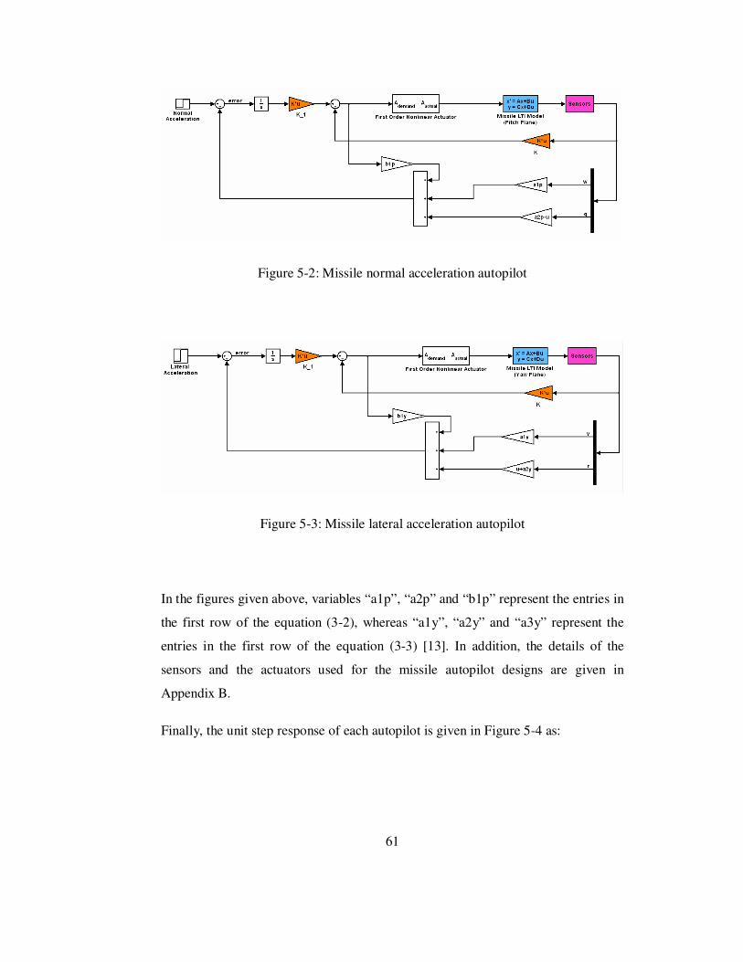
61

Figure 5-2: Missile normal acceleration autopilot

Figure 5-3: Missile lateral acceleration autopilot

In the figures given above, variables “a1p”, “a2p” and “b1p” represent the entries in

the first row of the equation (3-2), whereas “a1y”, “a2y” and “a3y” represent the

entries in the first row of the equation (3-3) [13]. In addition, the details of the

sensors and the actuators used for the missile autopilot designs are given in

Appendix B.

Finally, the unit step response of each autopilot is given in Figure 5-4 as:

62

0 0.2 0.4 0.6 0.8 10

0.2

0.4

0.6

0.8

1

1.2

1.4

time(s)

response

yaw acceleration (g)

roll (deg)

pitch acceleration (g)

Figure 5-4: Unit step responses of the missile autopilots

63

CHAPTER 6

GUIDANCE OF THE MISSILE

6.1 Introduction

In this chapter, formulations of three different missile guidance methods, one of

which is developed throughout this study, are given. In addition to the formulations,

these methods require some parameters to be selected before using them in the

simulation studies. Therefore, parameter selection processes and the necessary

assumptions are also given. Consequently, the engagement scenarios used for the

performance comparison of the guidance methods and the simulation results are

also given.

6.2 Proportional Navigation Guidance (PNG)

Theoretically, PNG guidance law gives out an acceleration command that is

proportional to LOS rate λ& and the missile-target closing velocity Vc [5]. The

acceleration command produced by PNG that is perpendicular to the instantaneous

missile-target LOS, can be stated as:

λ&cc NVn = , (6-1)

64

where, cn is the normal acceleration command, N is a unitless, designer chosen

gain (usually in the range of 3-5) known as the proportional navigation ratio, cV is

the missile-target closing velocity, and λ is the LOS angle.

In tactical IR missile applications of PNG, LOS rate is measured; whereas the

closing velocity is estimated [10] or taken as constant [3]. For the model used in this

thesis, LOS rate is calculated after the measurement of the position of the target.

The position measurement is obtained by adding a Gaussian noise with a specified

rms value to the position of the target since a seeker model does not exist in this

study.

Following figure shows two-dimensional missile-target engagement geometry to

illustrate how PNG works:

Figure 6-1: Two-dimensional missile-target engagement geometry

65

To derive relative kinematics between a missile and a target in the ECS, inertial

azimuth and elevation LOS angles are expressed respectively as:

+

−=

22tan

rr

r

EL

YX

Zaλ , (6-2)

( )rrAZ XYa ,2tan=λ , (6-3)

where, rY and

rZ denote the relative position errors and TMR stands for target-to-

missile range that can be expressed as:

222rrrTM ZYXR ++= . (6-4)

In order to use equation (6-1) to compute the accelerations in a non-rotating fixed

frame, cV should be clarified as:

TMc RV &−= . (6-5)

Once the equalities above are given, the guidance commands in the horizontal and

vertical frames can be stated respectively as:

cAZH VNa λ&= , (6-6)

cELV VNa λ&= . (6-7)

Proportional navigation ratio (N) is taken as 4 in this study.

66

6.3 Proportional Integral Derivative Navigation Guidance (PIDNG)

6.3.1 PIDNG Method Formulation

The PID controller design method can be applied from a different perspective to the

missile guidance problem [10]. It has a transfer function of the form:

sks

kksG d

ipc ++=)( , (6-8)

with the control input produced as:

)()()( sesGsu c= , (6-9)

where, )(se stands for the error to be regulated to zero. In the equation stated

above, controller input surely corresponds to steering command and error is the

LOS rate in order for the missile to hit the target.

By using the idea in equations (6-8) and (6-9) with the rule that LOS rate is the

variable to be nullified in guidance applications, the acceleration commands in the

vertical and horizontal planes of the inertial frame can be stated as follows:

ELdELiELpVdt

dkdtkka λλλ &&& ++= ∫ . (6-10)

AZdAZiAZpH

dt

dkdtkka λλλ &&& ++= ∫ . (6-11)

Here, the proportional (kp), integral (ki) and derivative (kd) navigation ratios are the

design parameters chosen by the user via trial-and-error. The following section

describes how these parameters were selected for the simulations done by PIDNG

method throughout the thesis.

67

6.3.2 Parameter (kp, ki, kd) Selection

In order to determine the proportional, integral and derivative navigation ratio

parameters of the PIDNG method, a fast maneuvering target scenario (S3, given in

the section 6.5.1.3) with a measurement rms value of 1 m is used. Also, for

guidance in the horizontal and the vertical planes of the inertial frame, the same

parameter set (kp, ki, kd) is used.

Table 6-1 shows the performance of the 13 different parameter sets. Considering the

results given in this table, if the miss distance is taken as the performance criterion,

the best values of the parameters are obtained at case 11. Therefore, for the rest of

the simulations where PIDNG is used in this thesis, proportional (kp), integral (ki)

and derivative (kd) navigation ratio parameters are used as 500, 10 and 0.1,

respectively. To illustrate the effect of these parameters on the trajectory of the

missile, three cases are chosen. The following figures give a feeling about how the

integral and derivative navigation ratios affect the trajectory and hence the miss

distance.

68

Table 6-1: Examples for PID parameter selection

Case kp ki kd Miss Distance (m) Time (s)

1 400 0 0 200.7 50.0

2 500 0 0 8.6 49.3

3 1000 0 0 53.9 41.4

4 1500 0 0 105.6 38.9

5 500 0.1 0 8.2 49.3

6 500 1 0 4.0 49.1

7 500 5 0 18.6 48.5

8 500 10 0 3.6 48.2

9 500 15 0 16.8 48.1

10 500 10 0.01 3.2 48.2

11 500 10 0.1 0.9 48.3

12 500 10 1 15.0 48.6

13 500 10 5 15.9 48.1

69

-1000 0 1000 2000 3000 4000 5000 6000 70000

500

1000

1500

2000

2500

3000

3500

y (m)

altitude (

m)

Missile and Target Trajectories in Inertial y-z Plane

Missile

Target

Figure 6-2: Case 4

-2000 0 2000 4000 6000 8000 100000

500

1000

1500

2000

2500

3000

3500

y (m)

altitude (

m)


Missile

Target

Figure 6-3: Case 7

70

-2000 0 2000 4000 6000 8000 100000

500

1000

1500

2000

2500

3000

3500

y (m)

altitude (

m)


Missile

Target

Figure 6-4: Case 11

6.4 Hybrid Proportional Navigation Guidance (HPNG)

PNG and PIDNG methods used in this thesis are based on the utilization of the

measured position of the target to calculate the closing velocity and the LOS rate.

These methods will suffer from the existence of the noise in the position

measurements, especially, when the rms error of measurements are high. Therefore,

an update in the calculated values of the closing velocity and the LOS rate is needed

to improve the guidance performance of the missile. To decrease the effect of noise

in the position measurements, a state estimator based on an Interacting Multiple

Model (IMM) via Kalman filtering (KF) approach is used. Since both measurement

and estimation values are utilized, this new method is called as “hybrid” PNG

method.

Considering the motion of the aircraft, resultant state trajectory of it involves

uniform motion and maneuvers. During all of the maneuvers, the missile’s tracking

performance should be high in order to decrease the miss-distance, the time of flight

71

and also the control effort used. So, the state estimation process is expected to give

better performance in estimated position rms error compared to the measured

position rms error. Also, the state estimator provides the velocity and acceleration

estimations of the target that are unavailable for PNG and PIDNG cases.

An IMM-KF state estimator can be constructed such that, the uniform motion and

the maneuvering motion of the target are modeled with the constant velocity (CV)

and constant acceleration (CA) kinematics models [4]. Since the acceleration of the

target being tracked is unknown for the missile sensor, it is modeled as a Gaussian

noise with zero mean. Variance of the Gaussian noise changes according to the

maneuver type being modeled, i.e.: noise with low variance is used for modeling the

CV motion whereas noise with higher variance is used for modeling the CA motion.

Also, CV and CA models are used in interaction such that the switching between

them is a Markov process (Markov chain) with known transition probabilities.

The details of the CV and CA models used in this thesis are formulated in the

following sections.

6.4.1 CV Model

The constant velocity (CV) motion model intends to represent the dynamics of a

platform in uniform motion that is not maneuvering. The noise term, which is zero-

mean white Gaussian, corresponds to the unknown target acceleration. The direct

discrete-time kinematics model representing the CV motion is given as follows:

kkkkk GvxFv

TI

IT

xI

TIIx +=

+

=+

3

3

2

3

331 20

(6-12)

where, T represents the constant time difference between the steps, I3 represents the

identity vector of dimension 3 and kv represents the unknown acceleration of the

target called process noise. Here, the state vector contains the position in x, y, z

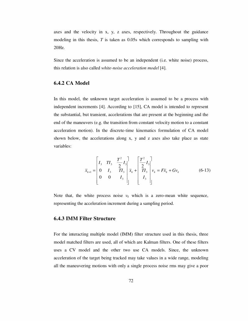
72

axes and the velocity in x, y, z axes, respectively. Throughout the guidance

modeling in this thesis, T is taken as 0.05s which corresponds to sampling with

20Hz.

Since the acceleration is assumed to be an independent (i.e. white noise) process,

this relation is also called white-noise acceleration model [4].

6.4.2 CA Model

In this model, the unknown target acceleration is assumed to be a process with

independent increments [4]. According to [15], CA model is intended to represent

the substantial, but transient, accelerations that are present at the beginning and the

end of the maneuvers (e.g. the transition from constant velocity motion to a constant

acceleration motion). In the discrete-time kinematics formulation of CA model

shown below, the accelerations along x, y and z axes also take place as state

variables:

kkkkk GvxFv

I

TI

IT

x

I

TII

IT

TII

x +=

+

=+

3

3

3

2

3

33

3

2

33

1

2

00

02

(6-13)

Note that, the white process noise vk which is a zero-mean white sequence,

representing the acceleration increment during a sampling period.

6.4.3 IMM Filter Structure

For the interacting multiple model (IMM) filter structure used in this thesis, three

model matched filters are used, all of which are Kalman filters. One of these filters

uses a CV model and the other two use CA models. Since, the unknown

acceleration of the target being tracked may take values in a wide range, modeling

all the maneuvering motions with only a single process noise rms may give a poor

73

performance. Instead, it is assumed that the target’s uniform motion can be modeled

with a single process (low) noise level and the maneuvering motion can be modeled

by using two different (higher) noise levels. The following table shows the

acceleration levels chosen to model the maneuvers done by the target.

Table 6-2: Process noise levels for the CV and CA models used

a_CV = 0.001 g,

a_CA1 = 0.01 g,

a_CA2 = 1 g.

a_CV : Acceleration level for the CV model

a_CAi : Acceleration increment level for the ith CA model, i = 1, 2

More details about the modeling of the IMM filter can be found in [4]. Briefly, the

steps used for the IMM filter are shown in the following figure:

74

Figure 6-5: One cycle of the IMM Estimator [4].

The mixing of the models is characterized by the Markov transition probabilities.

These probability values are assigned according to the properties of the dynamic

system (for instance the maneuverability of the target). By considering the

maneuvers expected to be done by the target, the Markov transition probabilities

can be chosen by the designer. Following matrix shows the Markov transition

probabilities that represent the switching between the CV and CA models used:

98.001.001.0

05.094.001.0

05.005.090.0

. (6-14)

The first row of this matrix shows the transition probabilities of CV model to stay

either in CV mode or switch to any of CA models. The total of these probabilities

must be 1. Usually, the diagonal entries of the matrix are chosen between 0.80 and

0.98 that shows the probability of each model to stay in its mode [4].

The IMM filter can be expressed by the following four fundamental steps [4], [15]:

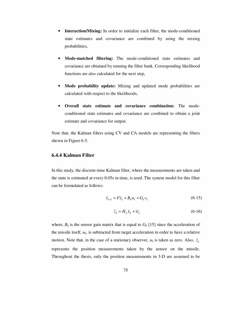
75

• Interaction/Mixing: In order to initialize each filter, the mode-conditioned

state estimates and covariance are combined by using the mixing

probabilities,

• Mode-matched filtering: The mode-conditioned state estimates and

covariance are obtained by running the filter bank. Corresponding likelihood

functions are also calculated for the next step,

• Mode probability update: Mixing and updated mode probabilities are

calculated with respect to the likelihoods,

• Overall state estimate and covariance combination: The mode-

conditioned state estimates and covariance are combined to obtain a joint

estimate and covariance for output.

Note that, the Kalman filters using CV and CA models are representing the filters

shown in Figure 6-5.

6.4.4 Kalman Filter

In this study, the discrete-time Kalman filter, where the measurements are taken and

the state is estimated at every 0.05s in time, is used. The system model for this filter

can be formulated as follows:

kkkkkk vGuBxFx ++=+1 (6-15)

kkkk wxHz += (6-16)

where, Bk is the sensor gain matrix that is equal to Gk [15] since the acceleration of

the missile itself, uk, is subtracted from target acceleration in order to have a relative

motion. Note that, in the case of a stationary observer, uk is taken as zero. Also, kz

represents the position measurements taken by the sensor on the missile.

Throughout the thesis, only the position measurements in 3-D are assumed to be

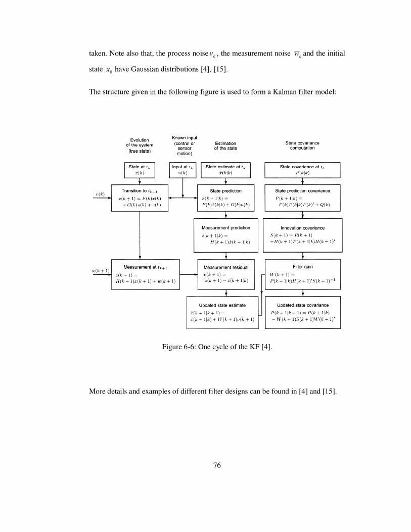
76

taken. Note also that, the process noise kv , the measurement noise kw and the initial

state 0x have Gaussian distributions [4], [15].

The structure given in the following figure is used to form a Kalman filter model:

Figure 6-6: One cycle of the KF [4].

More details and examples of different filter designs can be found in [4] and [15].

77

6.4.5 Formulation of the HPNG Method

The derivation of this new method is based on the PNG method. The only

modification to the acceleration commands generated by PNG is given as follows:

estcestestmeascmeasmeasc VNVNn ,, λλ && += (6-17)

where, the first part corresponds to the calculated values using the measurement,

and the second part corresponds to the calculated values using the estimation. In

fact, if the parameter Nest is chosen as zero, then this formulation is exactly in the

form of a PNG formulation. By modifying the PNG formulation with the results of

the estimations, an improvement is done if the estimation rms error is less than the

measurement rms error. Throughout this study, the following equation is used in

order to compare this new method with PNG fairly:

4=+ estmeas NN , (6-18)

where, Nmeas corresponds to the parameter N that is used in the equations (6-1), (6-

6) and (6-7).

If the estimated positions by the IMM filter are closer to the real position values

other than the measured position values, then the higher the Nest value, the more

effective the noise reduction in the signals used by the guidance system. As a

consequence, the guidance system that uses HPNG method will perform better than

the PNG method.

6.4.5.1 Selection of Nest

To select an appropriate value for Nest, HPNG method is tested on three different

scenarios defined in section 6.5.1. For these scenarios, different measurement noise

rms values (σw) are used to see the effectiveness of the state estimation process.

Here, σw represents the noise rms for each of three axes.

78

Table 6-3: Nest selection

σw = 1 m σw = 5 m σw = 10 m

S1 S2 S3 S1 S2 S3 S1 S2 S3

Miss Dist. (m) 10 6 4 675 820 213 3977 3506 3526

Nest = 0

Time (s) 44 36 49 37 30 40 8 11 11

Miss Dist. (m) 10 13 2 22 92 133 1969 684 486

Nest = 1.0

Time (s) 44 36 49 42 34 41 37 34 39

Miss Dist. (m) 10 24 3 54 25 87 409 857 456

Nest = 2.0

Time (s) 44 36 50 42 35 43 38 28 37

Miss Dist. (m) 12 31 5 33 59 134 447 47 393

Nest = 3.0

Time (s) 44 36 50 43 35 44 38 34 38

Miss Dist. (m) 18 34 1 12 148 121 19 196 108

Nest = 3.5

Time (s) 44 36 50 44 34 45 42 34 42

Miss Dist. (m) 19 35 5 131 79 40 21 154 130

Nest = 3.9

Time (s) 44 36 50 43 35 48 43 35 44

Miss Dist. (m) 18 32 11 136 82 27 200 34 51 Nest = 4.0

Time (s) 44 36 50 43 35 48 43 145 47

Remark: Throughout the study, miss distance represents the closest distance

between the missile and the aircraft trajectories (position states in 3D). Also, the

parameter, named “time”, given in Table 6-3 represents the time duration after

launch up to the instant when the miss distance is reached.

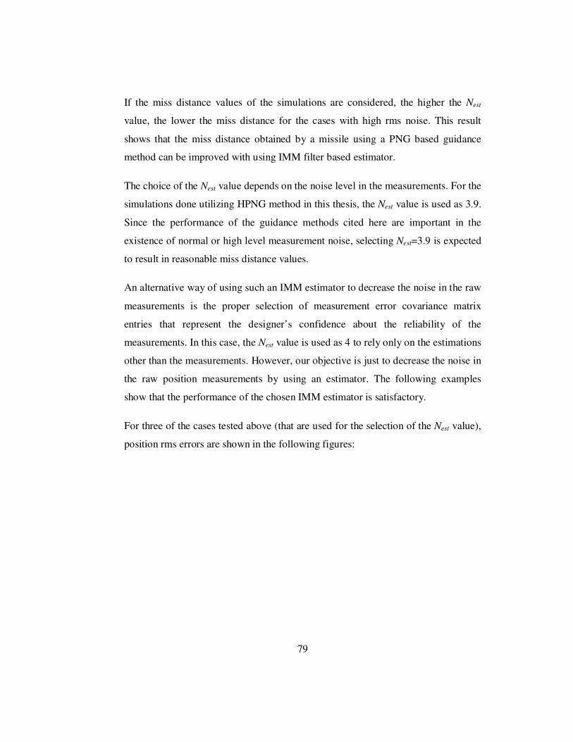
79

If the miss distance values of the simulations are considered, the higher the Nest

value, the lower the miss distance for the cases with high rms noise. This result

shows that the miss distance obtained by a missile using a PNG based guidance

method can be improved with using IMM filter based estimator.

The choice of the Nest value depends on the noise level in the measurements. For the

simulations done utilizing HPNG method in this thesis, the Nest value is used as 3.9.

Since the performance of the guidance methods cited here are important in the

existence of normal or high level measurement noise, selecting Nest=3.9 is expected

to result in reasonable miss distance values.

An alternative way of using such an IMM estimator to decrease the noise in the raw

measurements is the proper selection of measurement error covariance matrix

entries that represent the designer’s confidence about the reliability of the

measurements. In this case, the Nest value is used as 4 to rely only on the estimations

other than the measurements. However, our objective is just to decrease the noise in

the raw position measurements by using an estimator. The following examples

show that the performance of the chosen IMM estimator is satisfactory.

For three of the cases tested above (that are used for the selection of the Nest value),

position rms errors are shown in the following figures:

80

0 5 10 15 20 25 30 35 40 45 500

0.5

1

1.5

2

2.5

3

3.5

4

time (s)

pos

itio

n r

ms

err

or

(m)

Measurement

Estimation

Figure 6-7: Measurement and estimation errors for S3, Nest=3.9, σw=1 m

0 5 10 15 20 25 30 35 40 450

5

10

15

20

25

time (s)

positio

n r

ms e

rror

(m)

Measurement

Estimation


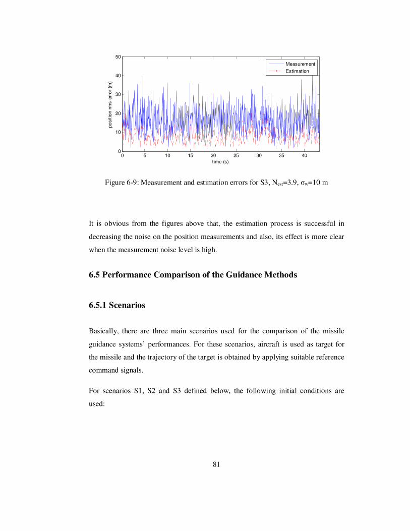
81

0 5 10 15 20 25 30 35 400

10

20

30

40

50

time (s)

po

sitio

n r

ms e

rror

(m)

Measurement

Estimation


It is obvious from the figures above that, the estimation process is successful in

decreasing the noise on the position measurements and also, its effect is more clear

when the measurement noise level is high.

6.5 Performance Comparison of the Guidance Methods

6.5.1 Scenarios

Basically, there are three main scenarios used for the comparison of the missile

guidance systems’ performances. For these scenarios, aircraft is used as target for

the missile and the trajectory of the target is obtained by applying suitable reference

command signals.

For scenarios S1, S2 and S3 defined below, the following initial conditions are

used:

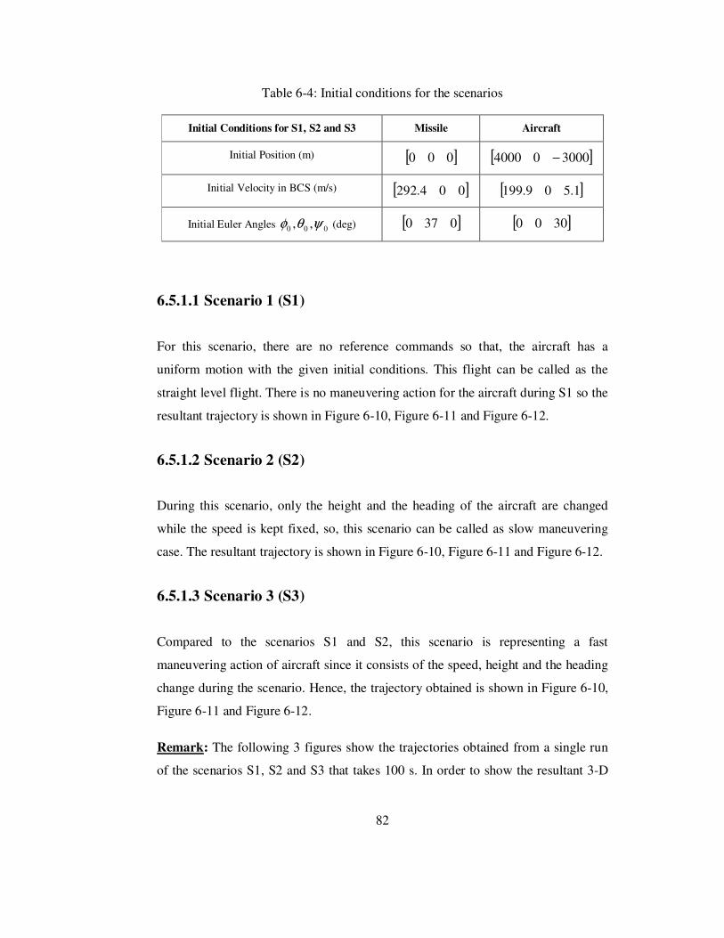
82

Table 6-4: Initial conditions for the scenarios

Initial Conditions for S1, S2 and S3 Missile Aircraft

Initial Position (m) [ ]000 [ ]300004000 −

Initial Velocity in BCS (m/s) [ ]004.292 [ ]1.509.199

Initial Euler Angles 000 ,, ψθφ (deg) [ ]0370 [ ]3000

6.5.1.1 Scenario 1 (S1)

For this scenario, there are no reference commands so that, the aircraft has a

uniform motion with the given initial conditions. This flight can be called as the

straight level flight. There is no maneuvering action for the aircraft during S1 so the

resultant trajectory is shown in Figure 6-10, Figure 6-11 and Figure 6-12.

6.5.1.2 Scenario 2 (S2)

During this scenario, only the height and the heading of the aircraft are changed

while the speed is kept fixed, so, this scenario can be called as slow maneuvering

case. The resultant trajectory is shown in Figure 6-10, Figure 6-11 and Figure 6-12.

6.5.1.3 Scenario 3 (S3)

Compared to the scenarios S1 and S2, this scenario is representing a fast

maneuvering action of aircraft since it consists of the speed, height and the heading

change during the scenario. Hence, the trajectory obtained is shown in Figure 6-10,

Figure 6-11 and Figure 6-12.

Remark: The following 3 figures show the trajectories obtained from a single run

of the scenarios S1, S2 and S3 that takes 100 s. In order to show the resultant 3-D

83

trajectories with a better sense of the maneuvers, output of the single run is given

from 3 different view angles.

01

23

x 104

0

1

2

3

x 104

0

1000

2000

3000

4000

y (m)

Target Trajectories in 3D

x (m)

altitude (

m)

S1

S2

S3

Figure 6-10: Aircraft trajectories for S1, S2 and S3 – 1st view angle

84

0

0.5

1

1.5

2

2.5

x 104

0

1

2

3

x 104

0

2000

4000

y (m)

Target Trajectories in 3D

x (m)

altitude (

m)

S1

S2

S3

Figure 6-11: Aircraft trajectories for S1, S2 and S3 – 2nd view angle

0 0.5 1 1.5 2 2.5

x 104

02

4

x 104

0

500

1000

1500

2000

2500

3000

3500 Target Trajectories in 3D

y (m)

x (m)

altitude (

m)

S1

S2

S3

Figure 6-12: Aircraft trajectories for S1, S2 and S3 – 3rd view angle

85

6.5.2 Simulation Results

In this section, the performance comparison is done for the PIDNG and HPNG

methods, since the PNG method performs worse than the HPNG method in the

existence of noise on the position measurements (see the section 6.4.5.1).

The three scenarios given in the previous section (S1, S2 and S3) were used with

different noise levels on the position measurement. Also, the success criterion is

taken as the 50 m kill distance, that is to say, miss distance values that are below 50

m are called as success for the evaluation of the missile guidance methods.

By checking the simulation results given in the following table, although both

methods have same success in most of the cases, performance of the new method,

HPNG, is higher when the measurement noise level is high. As a result, utilization

of the position values estimated by an IMM filter structure and then updating the

PNG method by combining the measurement and estimation results give way to a

new guidance method, which performs much better than the classical PNG method.

This new method, HPNG, even works better than the PIDNG method in some of the

scenarios when the measurement noise level is high.

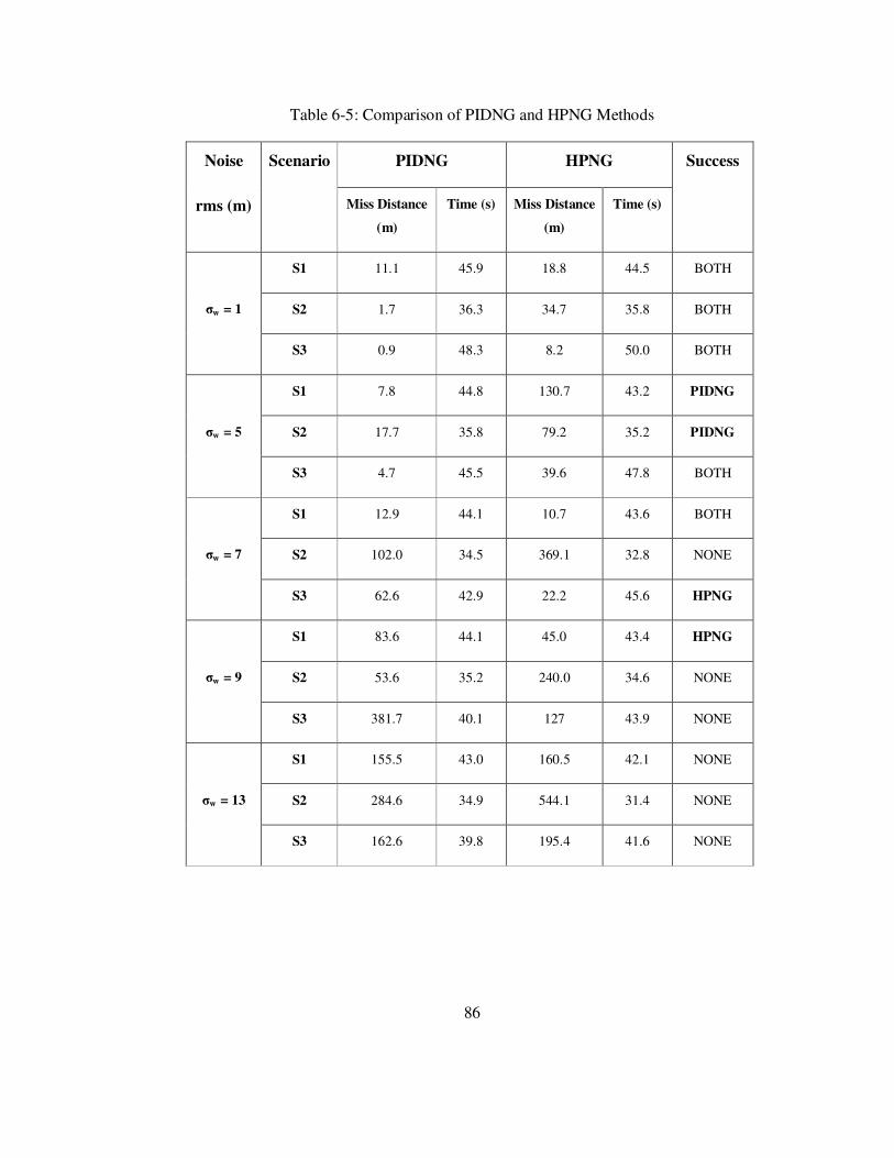
86

Table 6-5: Comparison of PIDNG and HPNG Methods

PIDNG HPNG Noise

rms (m)

Scenario

Miss Distance

(m)

Time (s) Miss Distance

(m)

Time (s)

Success

S1 11.1 45.9 18.8 44.5 BOTH

S2 1.7 36.3 34.7 35.8 BOTH σw = 1

S3 0.9 48.3 8.2 50.0 BOTH

S1 7.8 44.8 130.7 43.2 PIDNG

S2 17.7 35.8 79.2 35.2 PIDNG σw = 5

S3 4.7 45.5 39.6 47.8 BOTH

S1 12.9 44.1 10.7 43.6 BOTH

S2 102.0 34.5 369.1 32.8 NONE σw = 7

S3 62.6 42.9 22.2 45.6 HPNG

S1 83.6 44.1 45.0 43.4 HPNG

S2 53.6 35.2 240.0 34.6 NONE σw = 9

S3 381.7 40.1 127 43.9 NONE

S1 155.5 43.0 160.5 42.1 NONE

S2 284.6 34.9 544.1 31.4 NONE σw = 13

S3 162.6 39.8 195.4 41.6 NONE

87

CHAPTER 7

GUIDANCE OF THE AIRCRAFT

7.1 Introduction

To guide an aircraft under a missile threat such that the miss distance is maximized,

is a difficult problem and there is not a systematic way of solving such a problem.

According to some of the states (i.e. speed, direction, range) at the beginning of the

engagement scenario and also the dynamic limits of the aircraft and the missile, the

effective way of missile evasion technique for the aircraft is expected to change.

In this chapter, the aim is to develop a rule based missile evasion method to guide

the aircraft such that, the aircraft is successfully evaded by increasing the miss

distance. To do this, first, maximization of the miss distance is expressed as an

optimal control problem. After the optimal control problem is formulated and a

solution technique is given, this solution technique is applied on 45 cases that have

different initial conditions (in terms of the aircraft-missile distance, the relative

speed and direction at the beginning of the scenario). Then, by extracting a rule

from each of these cases, the reference signals of the aircraft autopilot is

determined. It is important to note that, these reference signals are the delta speed,

delta height and the delta yaw command signals.

Although these 45 cases are chosen to characterize the typical engagement

scenarios, a new optimal control problem with a different initial condition other

88

than these 45 cases should also be dealt with. Instead of solving the optimal control

problem for this new case, an interpolation method is formulated so that a solution

to a new case is found by combining the solutions of 45 cases by taking the distance

of the new case to all of the 45 cases into consideration. Since finding the solution

to an optimal control problem necessitates solving an adjoint system of differential

equations backward in time, its online implementation is unrealizable. However, the

proposed interpolation algorithm finds a solution online by combining the solutions

of the 45 optimal control problems that are solved offline.

Finally, formulation of a PNG-based guidance technique is given in order to

evaluate the performance of the proposed rule-based missile evasion method under

some simulations (that are given in the next Chapter).

7.2 Rule Based Missile Evasion Method

7.2.1 Miss Distance Maximization as an Optimal Control Problem

The optimal control problem for the miss distance maximization can be formulated

as follows:

)()(min)(

finalafinalmtu

tPtPJrr

−−= , (7-1)

subject to the equation (2-37) with the following constraints and the initial

condition:

0

maxmin

)0(

)(

0))((

xx

utuu

txG

=

≤≤

≤

, (7-2)

where, G(.) is a vector mapping of state inequality constraints, )( finalm tPr

and

)( finalm tPr

are the position of the missile and the aircraft at t=tfinal , minu and maxu are

89

the bounds of the control input vector. This problem is an optimal control problem

(with fixed final time) with state and input dependent inequality constraints. Thus,

instead of solving this problem analytically, nonlinear programming and simulation

tools are used in this thesis.

7.2.2 Typical Engagement Scenarios

Throughout this study, a typical engagement scenario is defined with the initial

distance between missile and aircraft, R (Figure 7-2), and the angle between the

initial velocity vectors of the missile and the aircraft, θ (Figure 7-1).

Figure 7-1: Missile and aircraft velocity vectors at the launch time

To illustrate the generic missile-aircraft engagement scenarios, the following figures

are given:

90

Figure 7-2: Generic engagement scenario for a missile and an aircraft - 1


91

For all of the cases chosen, the direction of aVr

is along the x-axis of the ECS. When

the distance between the missile and the aircraft, R, the initial altitude of the

aircraft, h, and the angle θ are given, the (xm,ym) coordinates of the missile launch

point are calculated with the following formula, assuming that the missile launch

point lies on the horizontal plane of ECS, with zm = 0 m:

222 sin

cos

hRy

Rx

m

m

−=

−=

θ

θ. (7-3)

From the formula above, it is seen that the xm takes both positive and negative

values according to the angle θ, however, ym only takes positive values. This

convention is used since (xm,-ym) coordinates are just the symmetric points with

respect to the x-z plane of the ECS. Using (xm,-ym) as the launch point instead of

(xm,ym) differs only in the lateral plane of the motion due to the symmetry of the

aircraft and the missile. The following figure shows the launch point that is

symmetric with the one shown in the previous figure.


92

In order to see the aircraft’s maneuvering capability for evasion, 5 different R and 9

different θ values are selected as follows:

{ }{ }170,150,130,110,90,70,50,30,10

3500,3000,2000,1000,500

=

=

θ

R, (7-4)

where, R is in meters and θ is in degrees and also total number of (R,θ)

combinations is 45.

Bu using the scenario and parameter definitions above, the following table is

obtained to summarize the conditions for all of the 45 cases:

Table 7-1: Engagement scenario parameters

Case # R (m) θ (deg) h (m) xm (m) ym (m) tfinal (s)

1 500 10 85 -492 18 3.46

2 500 30 85 -433 235 3.08

3 500 50 85 -321 373 2.55

4 500 70 85 -171 462 2.07

5 500 90 85 0 493 1.71

6 500 110 85 171 462 1.45

7 500 130 85 321 373 1.29

8 500 150 85 433 235 1.18

9 500 170 85 492 18 1.14

10 1000 10 170 -985 35 6.91

11 1000 30 170 -866 470 6.15

12 1000 50 170 -643 747 5.10

13 1000 70 170 -342 924 4.15

14 1000 90 170 0 985 3.42

15 1000 110 170 342 924 2.91

16 1000 130 170 643 747 2.57

17 1000 150 170 866 470 2.37

18 1000 170 170 985 35 2.27

19 2000 10 340 -1970 71 13.82

20 2000 30 340 -1732 940 12.31

21 2000 50 340 -1286 1494 10.21

22 2000 70 340 -684 1848 8.30

23 2000 90 340 0 1971 6.84

24 2000 110 340 684 1848 5.82

25 2000 130 340 1286 1494 5.14

93

Table 7-2: Engagement scenario parameters – cont’d

Case # R (m) θ (deg) h (m) xm (m) ym (m) tfinal (s)

26 2000 150 340 1732 940 4.74

27 2000 170 340 1970 71 4.54

28 3000 10 510 -2954 106 20.74

29 3000 30 510 -2598 1411 18.46

30 3000 50 510 -1928 2241 15.31

31 3000 70 510 -1026 2773 12.44

32 3000 90 510 0 2956 10.26

33 3000 110 510 1026 2773 8.73

34 3000 130 510 1928 2241 7.72

35 3000 150 510 2598 1411 7.10

36 3000 170 510 2954 106 6.82

37 3500 10 595 -3447 124 18.05

38 3500 30 595 -3031 1646 17.01

39 3500 50 595 -2250 2614 15.34

40 3500 70 595 -1197 3235 13.56

41 3500 90 595 0 3449 11.97

42 3500 110 595 1197 3235 10.72

43 3500 130 595 2250 2614 9.81

44 3500 150 595 3031 1646 9.23

45 3500 170 595 3447 124 8.95

For these 45 cases, the initial speed of the missile is taken as 292.4 m/s, the initial

speed of the aircraft for the cases 1-36 is taken as 150 m/s and for the cases 37-45, it

is taken as 100 m/s. This difference in the aircraft initial speed stems from the

constraint on the final time and the step size of the simulations in order for them to

be solvable with a powerful workstation (64 bit, 3.6 GHz processor with 8 MB

RAM). In addition, the final time of an engagement is calculated with the following

equation:

θcosam

final

VV

Rt rr

−= , (7-5)

94

where, the distance between the aircraft and the missile (at the launch time) is

divided by the difference of the missile and aircraft’s initial velocity vector

components along the LOS direction.

7.2.2.1 Solutions of the 45 Cases

7.2.2.1.1 Problem Solution Method

The formulation and the solution of the optimal control problem used in this thesis

are defined in [19].

The steps of the solution method used here is similar to the one used for the

optimization method explained in section 4.3. The basic differences are the state

and the input constraints and also the minimization here is applied on the aircraft

nonlinear model. So, “fmincon” function is used again to minimize the cost function

given in equation (7-1) subject to the following state and input constraints:

oo

oo

oo

oo

oo

oo

oo

oo

3030

5.215.21

2525

10

179179

179179

8989

1000

120000

3030

4510

/270/35

≤≤−

≤≤−

≤≤−

≤≤

≤≤−

≤≤−

≤≤−

≤≤

≤≤

≤≤−

≤≤−

≤≤

r

a

e

th

a

pow

mhm

smVsm

δ

δ

δ

δ

ψ

φ

θ

β

α

. (7-6)

Here, the position of the missile is obtained by taking the position states of the

missile designed in section 5.2 that uses the PNG method given in section 6.2.

95

During the simulations, measurement noise is not used, so both the missile and the

aircraft are assumed to have each other’s position information in the ECS.

Note that, the control input trim values calculated for the speed (Va) and altitude (h)

given for each case (by using the trimming algorithm defined in section 2.3) are

used as the initial conditions to start the minimization process.

By choosing a suitable termination condition, (i.e.: the directional derivative = 1e-6,

1-D search step length = 5e-4, maximum number of iterations = 150), the problem

is solved for all of the 45 cases successfully. Results of some of the cases are given

in the next section.

7.2.2.1.2 Results

All the 45 cases are solved with the proposed solution method given in the previous

section. The solution for each case is composed of the optimal control input vector

for the aircraft which is given in the equation (2-36). Note that, the time duration of

each control input vector is tfinal seconds, and it changes for each case.

The following 5 example cases show the resulting state trajectories after applying

the optimal control input vector to the nonlinear aircraft model:

96

-500

0

500

1000

-2000

0

2000

4000-200

0

200

400

y (m)

Missile and Target Trajectories in 3D

x (m)

altitude (

m)

Missile

Target

Figure 7-5: Case 20, miss distance = 720 m

-1000010002000

0

500

1000

0

100

200

300

400

x (m)

y (m)


altitude (

m)

Missile

Target


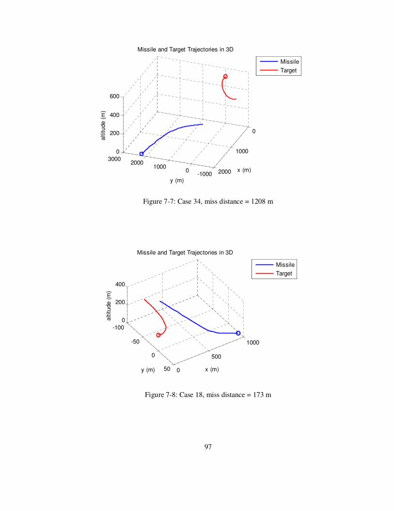
97

-10000

10002000

3000

0

1000

2000

0

200

400

600

x (m)


y (m)

altitude (

m)

Missile

Target


-100

-50

0

50 0

500

1000

0

200

400

x (m)


y (m)

altitude (

m)

Missile

Target


98

-50005001000

-500

0

500

1000

0

50

100

150

200

x (m)

y (m)


altitude (

m)

Missile

Target


7.2.2.2 Rule Extraction

Since the autopilot of the aircraft uses delta speed, delta height and delta yaw as the

command signals, the solution of each case, given in the previous section, must be

converted to delta speed, delta height and delta yaw commands. To do this, the

values of delta speed, delta height and delta yaw at t=0 is subtracted from their

values at t=tfinal. So, the optimal control input found for each case, iu , is converted to

a rule, ir , that is composed of the reference command signals of the aircraft

autopilot:

45,...,1,

)0()(

)0()(

)0()(

=

∆−∆

∆−∆

∆−∆

=

∆

∆

∆

= i

t

hth

VtV

h

V

r

ifinali

ifinali

ifinali

i

i

i

i

ψψψ

. (7-7)

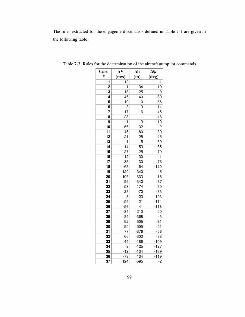
99

The rules extracted for the engagement scenarios defined in Table 7-1 are given in

the following table:

Table 7-3: Rules for the determination of the aircraft autopilot commands

Case #

∆V (m/s)

∆h (m)

∆ψ (deg)

1 12 1 -1

2 -1 -34 -10

3 -13 25 -9

4 -45 40 -60

5 -10 -10 36

6 -3 13 11

7 -17 6 -45

8 -23 11 46

9 -1 -3 10

10 55 -132 -2

11 45 -80 -30

12 21 -25 -45

13 1 5 -60

14 -14 -53 65

15 -27 -25 79

16 -12 30 1

17 -35 30 -75

18 -63 54 -120

19 120 -340 -5

20 105 -333 -16

21 95 -340 -37

22 58 -174 -69

23 28 -70 -83

24 3 -23 -103

25 -59 21 -114

26 -56 41 -118

27 -84 210 50

28 84 -368 -3

29 92 -505 -31

30 90 -505 -51

31 77 -376 -56

32 66 -300 -88

33 44 -186 -109

34 8 -125 -127

35 -12 -134 -139

36 -73 134 -119

37 124 -595 -2

100

Table 7-4: Rules for the determination of the aircraft autopilot commands – cont’d

Case #

∆V (m/s)

∆h (m)

∆ψ (deg)

38 133 -592 -25

39 126 -590 -32

40 118 -525 -68

41 83 -392 -83

42 83 -373 -110

43 58 -335 -129

44 33 -330 -142

45 8 -260 -174

Max. 133 210 79

Min. -84 -595 -174

7.2.3 Interpolation Algorithm

The function of the algorithm given here is to find a rule, r , for an arbitrary case

other than those 45 cases.

First, define the initial condition of each case given in the previous section as an

event, E . Each event can be defined by the initial distance between missile and

aircraft, R, and the initial angle between the velocity vectors of the missile and the

aircraft, θ:

45,,3,2,1, K=

= i

RE

i

i

i θ. (7-8)

Then, define the initial condition of an arbitrary case as an input event:

=

θ

RE . (7-9)

After that, distance of the arbitrary event to an event is defined as follows:

45,...,1, =−= iEEd ii . (7-10)

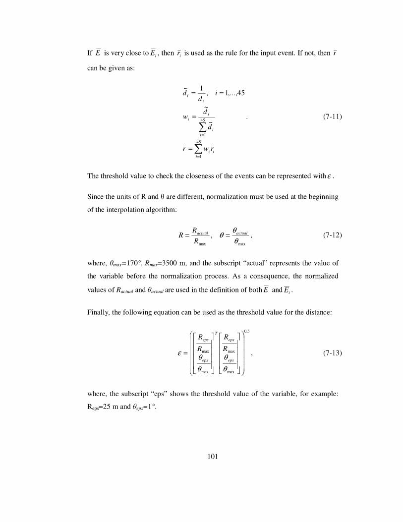
101

If E is very close to iE , then ir is used as the rule for the input event. If not, then r

can be given as:

i

i

i

i

i

i

i

i

i

rwr

d

dw

id

d

∑

∑

=

=

=

=

==

45

1

45

1

~

~

45,...,1,1~

. (7-11)

The threshold value to check the closeness of the events can be represented withε .

Since the units of R and θ are different, normalization must be used at the beginning

of the interpolation algorithm:

maxmax

,θ

θθ actualactual

R

RR == , (7-12)

where, θmax=170°, Rmax=3500 m, and the subscript “actual” represents the value of

the variable before the normalization process. As a consequence, the normalized

values of Ractual and θactual are used in the definition of both E and iE .

Finally, the following equation can be used as the threshold value for the distance:

5.0

max

max

max

max

=

θ

θ

θ

θε

eps

eps

T

eps

eps

R

R

R

R

, (7-13)

where, the subscript “eps” shows the threshold value of the variable, for example:

Reps=25 m and θeps=1°.

102

7.2.4 Implementation Details

During the implementation of the rule based missile evasion method, the

interpolation algorithm defined in the previous section is applied at every time step

of the simulation. Note that, the flight simulations throughout this thesis are run

with a fixed-step size of 10 ms.

Note that, since the formulated optimal control problem is complex, solving it with

a normal PC is not possible even the fixed-step size in the optimization process is

chosen large (i.e.: about 100 ms). Thus, a powerful workstation is needed to solve

this kind of a problem. It is obvious that, there is a compromise between the

duration of the engagement scenarios (tfinal) and the fixed step size of the

simulations. If the duration is increased, then large step size must be chosen to solve

it, and by choosing it large, the solution does not always converge.

7.3 Anti-Proportional Navigation Guidance (Anti-PNG)

7.3.1 Formulation

This guidance method is based on the PNG method which is explained in [20]. The

formulas given in section 6.2 for the PNG method are generally applicable with a

minor change in the sign of the produced acceleration commands. The main idea of

the anti-PNG method is to guide the aircraft with a command ( Tn in Figure 7-10)

which is the negative of the PNG command ( Tn′ in Figure 7-10). By doing this, the

aircraft is forced to evade from the missile instead of having a collision.

A 2-D aircraft-missile engagement geometry which is similar to the one given in

Figure 6-1 is given as follows:

103

Figure 7-10: Two-dimensional target-missile engagement geometry.

Equations (6-1) to (6-5) are directly used in order to formulate the anti-PNG

method. In addition, equations (6-6) and (6-7) are used with a negative sign as

shown below to express the guidance commands in the horizontal and vertical

frames, respectively:

cAZH VNa λ&−=′ , (7-14)

cELV VNa λ&−=′ . (7-15)

Note that, the proportional navigation ratio (N) is taken as 4 as in the case of PNG

method.

7.3.2 Conversion Logic

In order to use the anti-PNG method to guide the aircraft whose autopilot is

designed utilizing gain scheduled LQC method as expressed in section 4.2.5, the

104

outputs of the anti-PNG method, which are the acceleration commands, must be

converted to the autopilot reference commands that are delta speed, delta height and

delta yaw commands. To do this, the following steps are being followed:

1. The accelerations expressed in the ECS are converted to the delta speed

components that are expressed in the ECS:

dtaV

dtaV

Vz

Hy

∫

∫′=∆

′=∆. (7-16)

2. The delta speed components expressed in the ECS are converted to the delta

position components that are expressed in the ECS:

dtVz

dtVy

z

y

∫

∫∆=∆

∆=∆. (7-17)

3. The x-component of the aircraft speed that is expressed in the ECS is

assumed to be constant:

tVx

V

constV

x

x

x

∆=∆

=∆

⇒

≈

0

.

. (7-18)

4. The delta speed commands expressed in the ECS are converted to the WCS:

∆

∆

∆

=

∆

∆

∆

z

y

x

BEWB

z

y

x

V

V

V

TT

V

V

V

W

W

W

. (7-19)

Briefly, the autopilot commands that are obtained by using the assumption and the

equations above can be summarized as follows:

105

)arctan(

222

x

y

zh

VVVVWWW zyx

∆

∆=∆

∆−=∆

∆+∆+∆=∆

ψ

. (7-20)

Finally, note that the simulation studies in which the anti-PNG method is used are

given in the Chapter 8. There, the performance of the anti-PNG method is tested

under some example cases that are also used to test the performance of the rule

based missile evasion method given section 7.2.

106

CHAPTER 8

SIMULATION STUDIES

In this chapter, performances of the proposed aircraft guidance methods in chapter

7, rule-based method and anti-PNG method, are tested under 17 cases. These cases

are chosen to cover different ranges and orientations of the missile with respect to

the aircraft at the beginning of the engagement scenarios.

For each test case given in, missile-aircraft initial distance (R), initial angle between

missile and aircraft velocity vectors (θ), and aircraft height above ground (h) are

chosen first. Then, x-y position of the missile on the ground is calculated by using

equation (7-3). Note that, aircraft initial velocity vector lies along the x-axis of the

ECS and missile initial velocity vector lies along the initial LOS direction (see

Figure 7-3). In addition, initial speed of the missile is taken as 292.4 m/s and initial

speed of the aircraft is taken as 150 m/s.

Throughout the simulations, the missile is guided by the PNG method given in

section 6.2 and controlled by the autopilot that is designed in chapter 5. On the

other hand, the gain scheduled LQC structure designed in section 4.2.5 is used as

the aircraft autopilot. It is important to note that, both the aircraft and the missile are

assumed to know each other’s position during an engagement.

Results of the simulations are given in Table 8-2. Here, if a test scenario ends up

with a miss distance of 50 m or higher, the guidance method used is assumed to be

the successful, that is to say, the kill distance is chosen as 50 m.

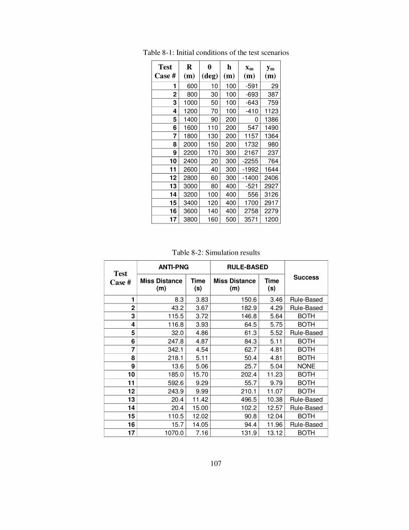
107

Table 8-1: Initial conditions of the test scenarios

Test Case #

R (m)

θ (deg)

h (m)

xm

(m) ym

(m) 1 600 10 100 -591 29

2 800 30 100 -693 387

3 1000 50 100 -643 759

4 1200 70 100 -410 1123

5 1400 90 200 0 1386

6 1600 110 200 547 1490

7 1800 130 200 1157 1364

8 2000 150 200 1732 980

9 2200 170 300 2167 237

10 2400 20 300 -2255 764

11 2600 40 300 -1992 1644

12 2800 60 300 -1400 2406

13 3000 80 400 -521 2927

14 3200 100 400 556 3126

15 3400 120 400 1700 2917

16 3600 140 400 2758 2279

17 3800 160 500 3571 1200

Table 8-2: Simulation results

ANTI-PNG RULE-BASED Test

Case # Miss Distance (m)

Time (s)

Miss Distance (m)

Time (s)

Success

1 8.3 3.83 150.6 3.46 Rule-Based

2 43.2 3.67 182.9 4.29 Rule-Based

3 115.5 3.72 146.8 5.64 BOTH

4 116.8 3.93 64.5 5.75 BOTH

5 32.0 4.86 61.3 5.52 Rule-Based

6 247.8 4.87 84.3 5.11 BOTH

7 342.1 4.54 62.7 4.81 BOTH

8 218.1 5.11 50.4 4.81 BOTH

9 13.6 5.06 25.7 5.04 NONE

10 185.0 15.70 202.4 11.23 BOTH

11 592.6 9.29 55.7 9.79 BOTH

12 243.9 9.99 210.1 11.07 BOTH

13 20.4 11.42 496.5 10.38 Rule-Based

14 20.4 15.00 102.2 12.57 Rule-Based

15 110.5 12.02 90.8 12.04 BOTH

16 15.7 14.05 94.4 11.96 Rule-Based

17 1070.0 7.16 131.9 13.12 BOTH

108

By checking the results given in Table 8-2, it is seen that there is only one critical

scenario (test case #9) in which both of the guidance methods are said to fail. But

for the rest of the test scenarios, the rule based method is successful to guide the

aircraft by evading the missile, whereas for the 6 of the scenarios, anti-PNG method

is said to fail. However, for 8 of the scenarios at which both of the methods are said

to be successful, miss distance values obtained by the anti-PNG method are higher

than the values obtained by the rule-based method. This result shows that the anti-

PNG method may also be used as an effective guidance method for some specific

scenarios.

If the kill distance of 50 m is used as the only success criterion, following

generalizations can be deduced:

• For the short range engagements (500-1500 m), and the long range

engagements (3000-4000 m) rule based method performs better than the

anti-PNG method,

• For the mid-range engagements (1500-3000 m), both methods perform well

except a specific case which is test case #9 (a mid-range, nearly head-on

engagement).

In order to make more generalizations, the test case parameter resolutions may be

increased and also different PNG ratios can be used for the anti-PNG method to

check its effect on the evasion capability of the aircraft.

The missile and the aircraft trajectories in 3-D, obtained for both guidance methods

applied on each test case (given in Table 8-2) are shown as follows:

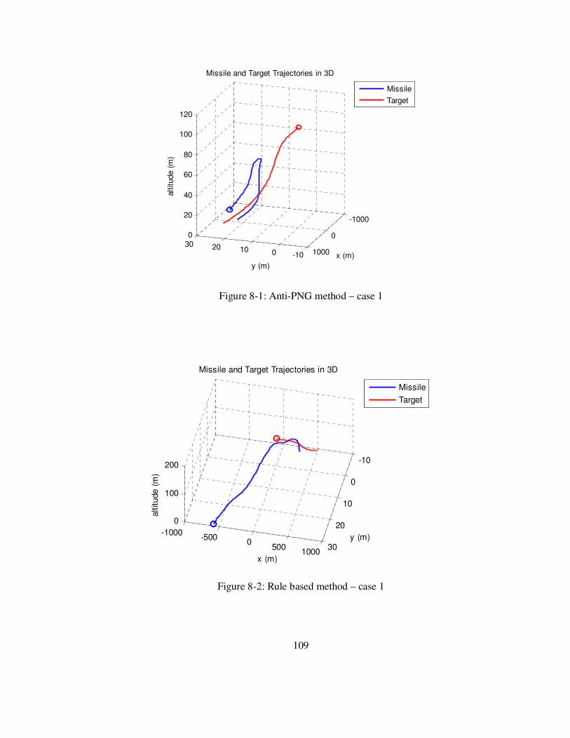
109

-100102030

-1000

0

1000

0

20

40

60

80

100

120

x (m)


y (m)

altitude (

m)

Missile

Target

Figure 8-1: Anti-PNG method – case 1

-10

0

10

20

30

-1000-500

0500

1000

0

100

200

y (m)

x (m)


altitude (

m)

Missile

Target

Figure 8-2: Rule based method – case 1

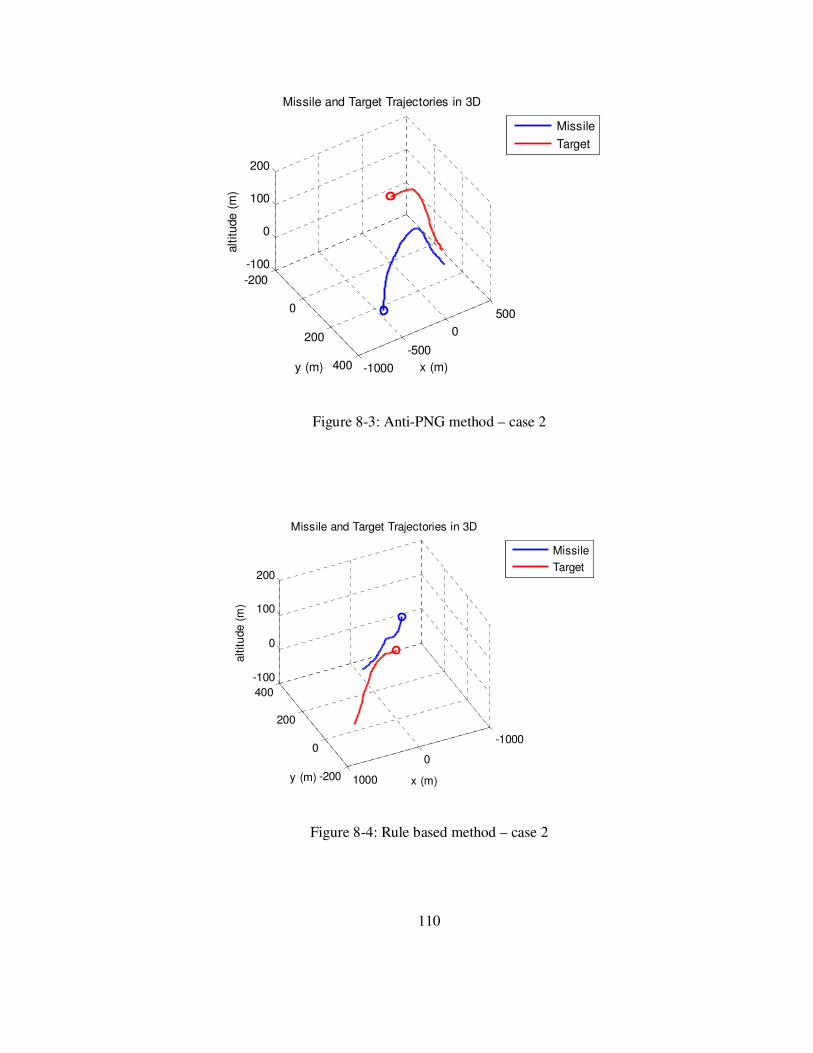
110

-200

0

200

400 -1000

-500

0

500

-100

0

100

200

x (m)


y (m)

altitude (

m)

Missile

Target


-200

0

200

400

-1000

0

1000

-100

0

100

200

x (m)


y (m)

alt

itu

de (

m)

Missile

Target


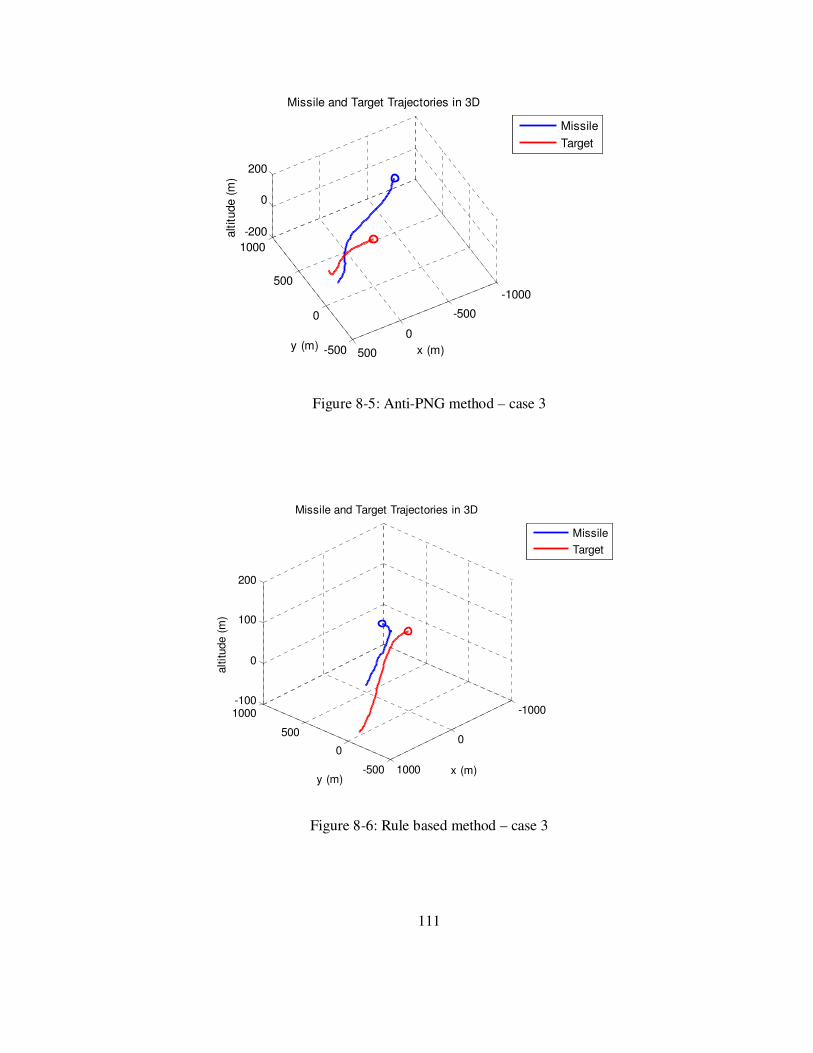
111

-500

0

500

1000

-1000

-500

0

500

-200

0

200

x (m)


y (m)

altitude (

m)

Missile

Target


-500

0

500

1000 -1000

0

1000

-100

0

100

200

x (m)


y (m)

altitude (

m)

Missile

Target


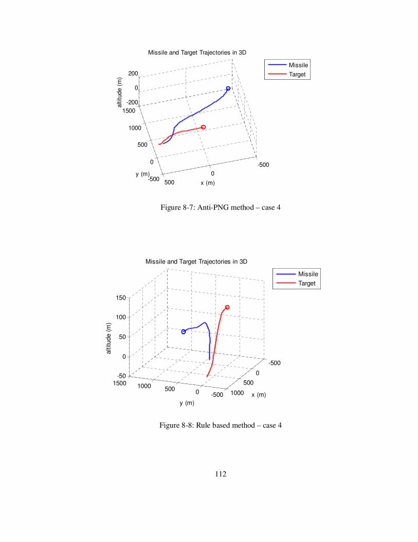
112

-500

0

500

1000

1500

-500

0

500

-200

0

200

x (m)


y (m)

altitude (

m)

Missile

Target


-500050010001500

-500

0

500

1000

-50

0

50

100

150

x (m)


y (m)

altitude (

m)

Missile

Target


113

-1000

0

1000

2000

0

500

10000

100

200

300

y (m)


x (m)

altitude (

m)

Missile

Target


-5000500100015000

5001000

0

50

100

150

200

250

x (m)


y (m)

altitude (

m)

Missile

Target


114

-500050010001500

05001000

-50

0

50

100

150

200

250 Missile and Target Trajectories in 3D

y (m)x (m)

altitude (

m)

Missile

Target


-10000

10002000

0

500

1000

0

50

100

150

200

250

y (m)


x (m)

altitude (

m)

Missile

Target


115

-5000

5001000

1500

0

500

1000

1500

-100

0

100

200

300

y (m)


x (m)

altitude (

m)

Missile

Target


-10000

10002000 0

1000

20000

100

200

300

x (m)


y (m)

altitude (

m)

Missile

Target


116

-5000

5001000

1500

0

500

1000

1500

-100

0

100

200

300

y (m)


x (m)

altitude (

m)

Missile

Target


-5000

500

1000 0

1000

20000

100

200

300

x (m)


y (m)

altitude (

m)

Missile

Target


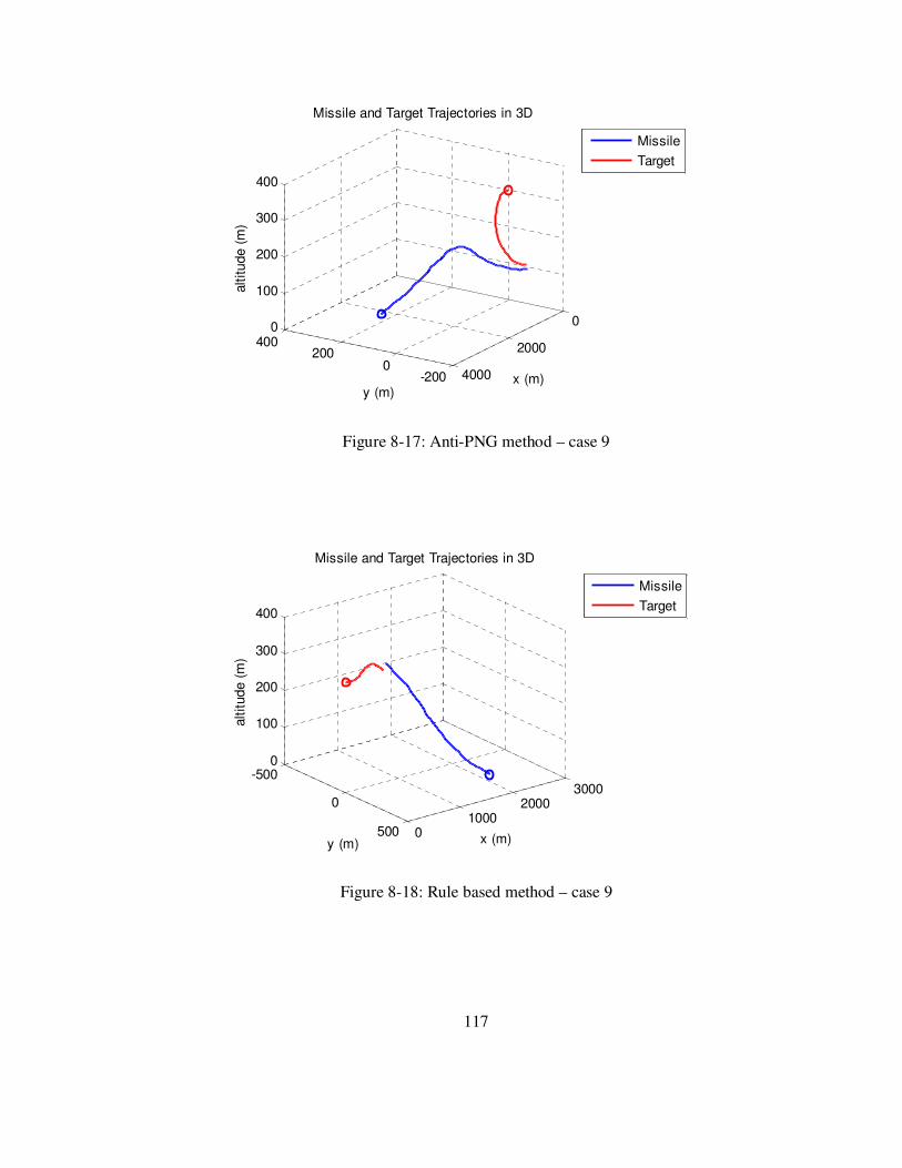
117

-2000

200400

0

2000

4000

0

100

200

300

400

x (m)


y (m)

altitude (

m)

Missile

Target


-500

0

500 01000

20003000

0

100

200

300

400

x (m)


y (m)

altitude (

m)

Missile

Target


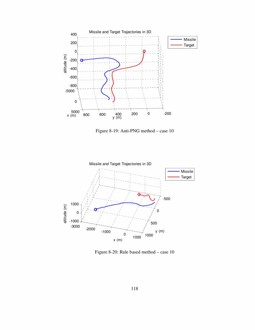
118

-2000200400600800

-5000

0

5000

-800

-600

-400

-200

0

200

400


y (m)

x (m)

altitude (

m)

Missile

Target


-500

0

500

1000

-3000-2000

-10000

1000

-1000

0

1000

y (m)

x (m)


altitude (

m)

Missile

Target


119

-2000200400600800

-5000

0

5000

-800

-600

-400

-200

0

200

400


y (m)

x (m)

altitude (

m)

Missile

Target


-2000

0

2000-2000 -1000 0 1000

0

100

200

300

400

x (m)


y (m)

altitude (

m)

Missile

Target


120

-5000

0

5000

-1500-1000-50005001000

-100

0

100

200

300


x (m)

y (m)

altitude (

m)

Missile

Target


-5000

0

5000

-1500-1000-5000500-500

0

500

1000

y (m)


x (m)

altitude (

m)

Missile

Target


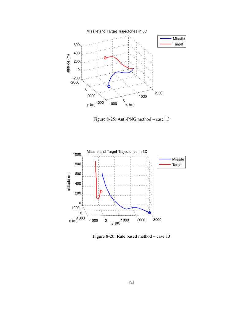
121

-2000

0

2000

4000 -10000

10002000

-200

0

200

400

600

x (m)


y (m)

altitude (

m)

Missile

Target


-1000 0 1000 2000 3000-1000

0

1000

0

200

400

600

800


y (m)

x (m)

altitude (

m)

Missile

Target


122

-5000

0

5000

0500

10001500

2000

0

200

400

600

y (m)


x (m)

altitude (

m)

Missile

Target


-20000200040000

5001000

0

200

400

600

800

1000

1200

x (m)


y (m)

altitude (

m)

Missile

Target


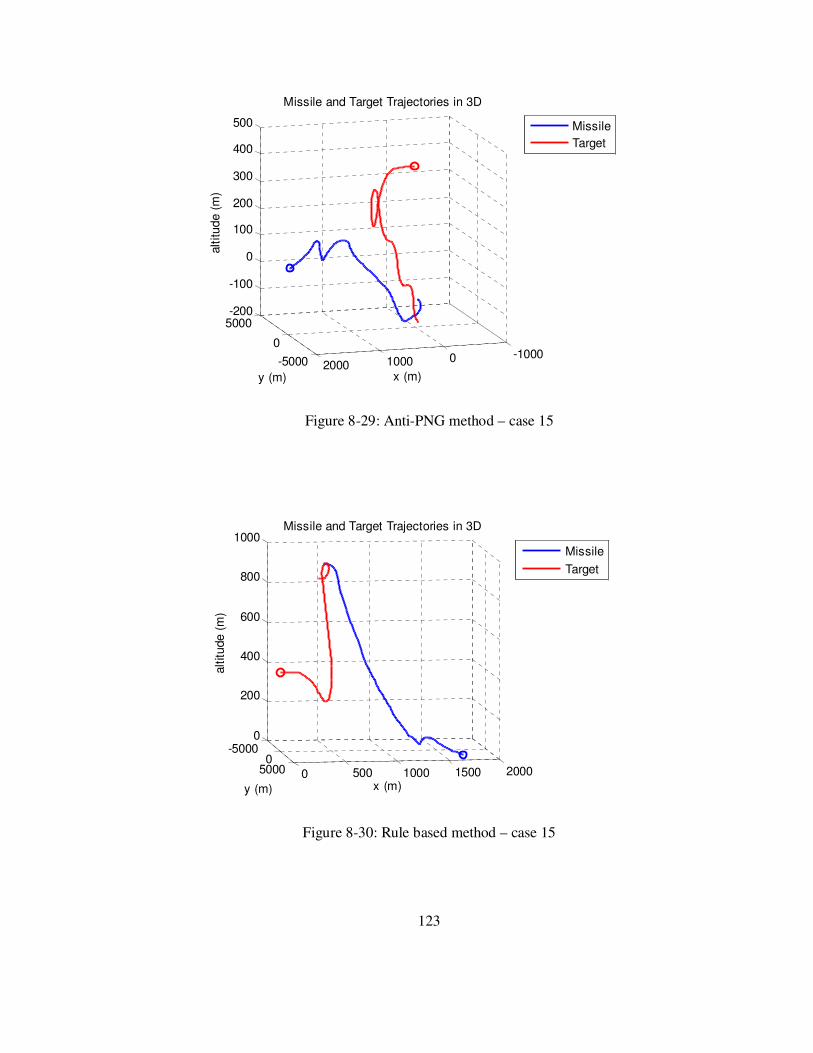
123

-5000

0

5000

-1000010002000

-200

-100

0

100

200

300

400

500

x (m)


y (m)

altitude (

m)

Missile

Target


-50000

5000 0 500 1000 1500 2000

0

200

400

600

800


x (m)y (m)

altitude (

m)

Missile

Target


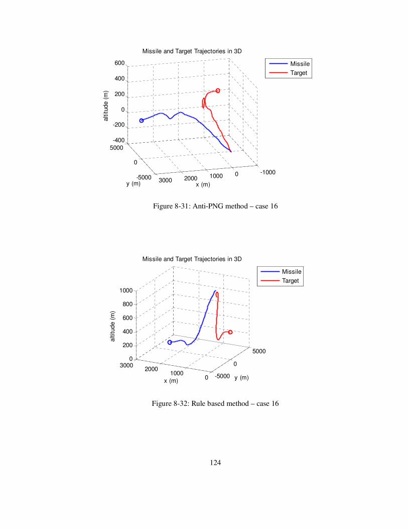
124

-5000

0

5000

-10000100020003000

-400

-200

0

200

400

600

x (m)


y (m)

altitude (

m)

Missile

Target


-5000

0

5000

01000

20003000

0

200

400

600

800

1000

y (m)


x (m)

altitude (

m)

Missile

Target


125

-2000

0

2000

01000200030004000

0

200

400


x (m)y (m)

altitude (

m)

Missile

Target


-10000

10002000

0

2000

4000

-200

0

200

400

600

y (m)


x (m)

altitude (

m)

Missile

Target


126

CHAPTER 9

CONCLUSION AND FUTURE WORK

In this thesis, in order to develop a guidance system for a missile and an aircraft,

first, the derivations of EOM of a missile and an aircraft are given. Then,

linearization, trimming and decoupling processes of the nonlinear EOM are

explained. After having the linearized models, the controllers are designed based on

the lateral and the longitudinal LTI models separately. The aircraft controllers are

tested on both LTI system and NL system, whereas, the missile controllers are only

tested on the LTI system. Then, the guidance system designs for a missile and an

aircraft are explained. Finally, simulation studies are given in order to compare the

performances of the proposed aircraft guidance methods.

The main contribution of this thesis to the literature is two new guidance methods,

one of which is developed for a missile and the other is developed for a fighter

aircraft. Although the new missile guidance method, HPNG, is based on the

classical PNG method, its performance is much better than the performance of the

PNG method, especially when there is noise in the position measurements.

Performance of the HPNG method may further be improved by using more complex

Kalman filter structures that are suppressing the measurement noise more and also

modeling the target maneuvers better.

The aircraft guidance method developed for this study is the rule based missile

evasion method that suggests a way of using the results of the miss distance

127

maximization problem online, although the problem is formulated as an optimal

control problem and the online implementation of solving such a problem is

unrealizable. Therefore, an interpolation algorithm finds a solution online by

combining the solutions of the 45 optimal control problems that are solved offline.

Hence, the aircraft is guided online by using the interpolated rule derived from the

solution of lots of miss distance maximization problems that are constructed taking

the typical engagement scenarios into account.

A relatively new guidance method used for the aircrafts given in [20], called anti-

PNG, is utilized for this study with a suitable conversion logic. This guidance

method is used to evaluate the performance of the rule based method by comparing

them under some generic engagement scenarios. The main idea of the anti-PNG

method is to guide the aircraft with a command which is the negative of the PNG

command. By doing this, the aircraft is forced to evade from the missile instead of

having a collision.

Simulation studies given in chapter 8 shows that the rule based missile evasion

algorithm performs better than the anti-PNG method. However, the simulation

results also show that the anti-PNG method may also be used as an effective

guidance method for some specific scenarios.

In addition to the studies done in this thesis, both of the proposed aircraft guidance

methods may further be improved. For example, the rule based method developed

here is used to extract general rules (change in speed, height and yaw). An

improvement can be made such that a collection of some special purpose rules that

behaves as a general purpose rule is found for a more complex engagement scenario

that includes CMs (such as a flare) and CCMs (such as a tracker that discards the

CMs). Another improvement may be made by solving much more optimal control

problems to increase the resolution in the rule extraction process. On the other hand,

the conversion logic used for the anti-PNG method may be improved to evade from

a proportional navigation guided threat in a more effective way.

128

Finally, all the suggested improvements for the given guidance methods may be

considered as a future work that constitutes the parts of a doctoral study.

129

REFERENCES

[1] K. Ogata, “Modern Control Engineering”, Prentice Hall, NJ, 2002

[2] B. Stevens, and F. Lewis, “Aircraft Control and Simulation”, Wiley

Interscience, NY, 1992

[3] P. H. Zipfel, “Modeling and Simulation of Aerospace Vehicle Dynamics”,

AIAA Education Series, VA, 2000

[4] Y. Bar-Shalom, X. R. Li, and T. Kirubarajan, “Estimation with Applications to

Tracking and Navigation”, John Wiley & Sons, NY, 2001

[5] P. Zarchan, “Tactical and Strategic Missile Guidance”, Volume 199, Progress in

Astronautics and Aeronautics, Massachusetts, 2002

[6] L. T. Nyugen, M. E. Ogburn, W. P. Gilbert, K. S. Kibler, P. W. Brown, and P.

L. Deal, “NASA Technical Paper 1538 – Simulator Study of Stall / Post-Stall

Characteristics of a Fighter Airplane With Relaxed Longitudinal Static Stability”,

NASA, Langley, 1979

[7] F. R.Garza, and E. A. Morelli, “A Collection of Nonlinear Aircraft Simulations

in MATLAB”, NASA/TM-2003-212145, Virginia, 2003

[8] Y. Huo, “Model of F-16 Fighter Aircraft”,

http://www.usc.edu/dept/ee/catt/soft.htm, June 10th 2007, Last date accessed:

January 15th 2008

[9] R. S. Russell, “Nonlinear F-16 Simulation Using Simulink and Matlab”,

Technical Report, Department of Aerospace Engineering and Mechanics,

University of Minnesota, 2003,

130

http://www.aem.umn.edu/people/faculty/balas/darpa_sec/SEC.Software.html,

February 10th 2007, Last date accessed: January 15th 2008

[10] Ç. Evcimen, and K. Leblebicioğlu, “An Optimal Proportional-Integral

Guidance for Missiles”, 4. Ankara International Aerospace Conference, 10-12

September 2007

[11] M. Rauw, S. Bennani, H. van der Vaart, “An Integrated Approach to the

Design of Flight Control Systems using CAD Tools”, 3rd ESIEE Congress, France,

November 17-18, 1994

[12] http://www.mathworks.com, February 1st 2007, Last date accessed: May 2nd

2008

[13] R. Ö. Doruk, “Missile Autopilot Design by Projective Control Theory”, M. S.

Thesis in METU, Department of Electrical and Electronics Engineering, August

2003

[14] K. D. Şahin, “A Pursuit Evasion Game Between a Missile and an Aircraft”, M.

S. Thesis in METU, Department of Electrical and Electronics Engineering,

December 2002

[15] B. Yıldırım, “A Comparative Evaluation of Conventional and Particle Filter

Based Radar Target Tracking”, M. S. Thesis in METU, Department of Electrical

and Electronics Engineering, November 2007

[16] J. H. Blakelock, “Automatic Control of Aircraft and Missiles”, John Wiley &

Sons, NY, 2nd Edition, 1991

[17] D. E. Kirk, “Optimal Control Theory: An Introduction”, Prentice-Hall, NJ,

1970

[18] C. T. Chen, “Linear System Theory and Design”, 3rd Ed, Oxford University

Press, NY, 1999

131

[19] V. M. Becerra, “Solving Optimal Control Problems with State Constraints

Using Nonlinear Programming and Simulation Tools”, IEEE Transactions on

Education Vol. 47, No. 3, August 2004

[20] B. Jung, K. S. Kim, Y. Kim, “Guidance Law for Evasive Aircraft Maneuvers”,

AIAA Guidance, Navigation and Control Conference and Exhibit, Austin, Texas,

11-14 August 2003

132

APPENDIX A. AIRCRAFT DESIGN PARAMETERS

A.1 Aerodynamic Model and Coefficients

Aerodynamic forces and moments stem from the air diverted by the aircraft in

different directions, depending on the following factors:

• the airspeed VT (or Mach number M) and density of the airflow ρ,

• the geometry of the aircraft: wing area S, wing span b and mean

aerodynamic chord c ,

• the orientation of the aircraft relative to the airflow: angle of attack α and

angle of sideslip β,

• the chord surface deflections δ,

• the angular rates p, q , r.

As a result of these dependencies, non-dimensional aerodynamic force and moment

coefficients of the aircraft vary nonlinearly with angle of attack and sideslip,

angular velocity components and control surface deflections. There are other

variables such as the time derivatives of the angle of attack and sideslip that also

play a role, but this effect is neglected because of the Assumption 1. Detailed

information about the aerodynamic forces and moments is given in [2].

Briefly, the standard way of modeling the aerodynamic forces and moments can be

given as follows:

133

,...),,,,,(

,...),,,,,(

,...),,,,,(

δβα

δβα

δβα

rqpSCqZ

rqpSCqY

rqpSCqX

T

T

T

Z

Y

X

=

=

=

, (A-1)

,...),,,,,(

,...),,,,,(

,...),,,,,(

δβα

δβα

δβα

rqpSbCqN

rqpCcSqM

rqpSbCqL

T

T

T

n

m

l

=

=

=

, (A-2)

where, q is the aerodynamic pressure (see Appendix A.2). Instead of the BCS force

coefficientsTXC ,

TYC andTZC , the WCS force coefficients DC , YC and LC can be

used, where DC is called drag, YC is side-force and LC is lift coefficient [2]. All of

these aerodynamic coefficients can be obtained by wind-tunnel experiments and

flight tests. The aerodynamic data used for the aircraft in this thesis were derived

from wind-tunnel tests conducted with sub-scaled models of a jet fighter aircraft,

which is F-16 [6].

Below, formulations of total coefficient equations are shown that are formed by

summation of various aerodynamic contributions to a given coefficient [2]:

The x-axis force coefficientTXC :

)(2

),( dX

T

edxX qTC

V

cqCC αδα += . (A-3)

The y-axis force coefficientTYC :

[ ]pCrCV

bC dYdY

T

radY prT

)()(230

086.020

021.002.0 ααδδ

β ++++−= . (A-4)

The z-axis force coefficientTZC :

25

19.0)(2

),(1,e

dZ

T

ddzZ qTC

V

cqCC

δαβα −+= . (A-5)

134

The rolling-moment coefficientTl

C :

[ ] )30

)(,()20

)(,()()(2

),( 3,2,1,r

ddla

ddldldl

T

ddll CCpCrCV

bCC

prT

δβα

δβαααβα ++++= . (A-6)

The pitching moment coefficientTmC :

)(2

)(),( dm

T

cgcgrZedmm qTTC

V

cqxxCCC αδα +−+= . (A-7)

The yawing moment coefficientTnC :

[ ]

)30

)(,()20

)(,(

)...()()(2

),(

3,2,

1,

r

ddn

a

ddn

cgcgrYdndn

T

ddnn

CC

xxCb

cpCrC

V

bCC

TprT

δβα

δβα

ααβα

++

−−++=

, (A-8)

where, dα and dβ represent α and β in degrees. Note that, xcgr is the reference

center of gravity as a fraction of c and xcg is the center of gravity as a fraction of c ,

whose values are taken as 0.35 and 0.30, respectively [2].

The data for the aerodynamic coefficients are given as look-up tables in [2], and it is

valid for the following flight envelope for the F-16 [6], [2] and [7]:

• -10° ≤ α ≤ 45°

• -30° ≤ β ≤ 30°

• 0.1 ≤ M ≤ 0.6

• 0 m ≤ h ≤ 15,239 m

where, M is the Mach number (see Appendix A.2) and h is the altitude. During the

aircraft flight simulations, a linear interpolation algorithm is used to calculate the

135

coefficients within the flight envelope that also extrapolates beyond the look-up

table boundaries, however, the results are more likely to be unrealistic.

A.2 Atmospheric Model

Air density and speed of sound are calculated using relations that formulate the U.S.

Standard Atmosphere [2], [8]. Required quantities that depend on these atmospheric

properties, namely, Mach number M and dynamic pressure q are also calculated.

The relationships are:

2

14.4

5

5.0

000,355193.17164.1

000,353903.17164.1

002377.0

10703.01

T

T

T

Vq

fthT

V

fthV

M

T

hT

ρ

ρ

=

<×××

≥××=

×=

×−= −

, (A-9)

where, T is the temperature in Kelvin, h is the height in feet, ρ is the air density in

slug/ft3, VT is the true airspeed in ft/s and q is in lbf/ft2.

A.3 Engine Model

The jet fighter aircraft is powered by an afterburning turbofan jet engine, which is

modeled taking throttle gearing and engine power level lag into account. Thrust

response is modeled with a first-order lag, and lag time constant engτ is modeled as

a function of the actual engine power level aP and the commanded power, cP . The

commanded power level changes linearly with the throttle position up to the level of

0.77 and then the change of the slope causes nonlinearity as seen below [6]:

>−

≤=

77.038.11738.217

77.094.64)(

thth

thth

thcif

ifP

δδ

δδδ . (A-10)

136

Note that, the throttle position is limited to the range 10 ≤≤ thδ . As mentioned

before, engine power level dynamic response is modeled using a first-order lag.

Therefore, actual power level derivative aP& is given by [6]:

)(1 *

ac

eng

a PPP −=τ

& , (A-11)

where

<<

≥<

<≥

≥≥

=

5050

505040

505060

5050

*

acc

ac

ac

acc

c

PandPifP

PandPif

PandPif

PandPifP

P , (A-12)

<<

≥<

<≥

≥≥

=

50501

50500.5

50501

50500.5

1

ac

T

ac

ac

T

ac

eng

PandPif

PandPif

PandPif

PandPif

τ

τ

τ, (A-13)

<−<−−

≥−

≤−

=

50)(25)(036.09.1

50)(1.0

25)(0.11

**

*

*

acac

ac

ac

TPPifPP

PPif

PPif

τ. (A-14)

Engine thrust data for idle idleT , military milT and maximum power settings maxT are

given in look-up table format as a function of altitude and Mach number over

ranges 0 m < h < 15,239 m and 0 ≤ M ≤ 1 and the resulting force produced by the

thrust is computed according to the actual engine power level as follows [6]:

≥−

−+

<−+=

50)50

50)((

50)50

)((

max aa

milmil

aa

idlemilidle

T

PifP

TTT

PifP

TTTF . (A-15)

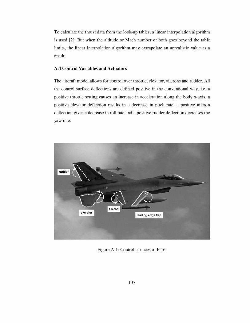
137

To calculate the thrust data from the look-up tables, a linear interpolation algorithm

is used [2]. But when the altitude or Mach number or both goes beyond the table

limits, the linear interpolation algorithm may extrapolate an unrealistic value as a

result.

A.4 Control Variables and Actuators

The aircraft model allows for control over throttle, elevator, ailerons and rudder. All

the control surface deflections are defined positive in the conventional way, i.e. a

positive throttle setting causes an increase in acceleration along the body x-axis, a

positive elevator deflection results in a decrease in pitch rate, a positive aileron

deflection gives a decrease in roll rate and a positive rudder deflection decreases the

yaw rate.

Figure A-1: Control surfaces of F-16.

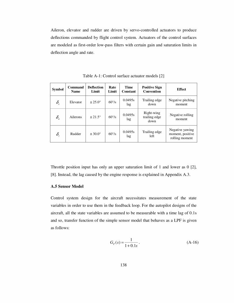
138

Aileron, elevator and rudder are driven by servo-controlled actuators to produce

deflections commanded by flight control system. Actuators of the control surfaces

are modeled as first-order low-pass filters with certain gain and saturation limits in

deflection angle and rate.

Table A-1: Control surface actuator models [2]

Symbol Command

Name Deflection

Limit Rate Limit

Time Constant

Positive Sign Convention

Effect

eδ Elevator ± 25.0° 60°/s 0.0495s

lag Trailing edge

down Negative pitching

moment

aδ Ailerons ± 21.5° 60°/s 0.0495s

lag

Right-wing trailing edge

down

Negative rolling moment

rδ Rudder ± 30.0° 60°/s 0.0495s

lag Trailing edge

left

Negative yawing moment, positive rolling moment

Throttle position input has only an upper saturation limit of 1 and lower as 0 [2],

[8]. Instead, the lag caused by the engine response is explained in Appendix A.3.

A.5 Sensor Model

Control system design for the aircraft necessitates measurement of the state

variables in order to use them in the feedback loop. For the autopilot designs of the

aircraft, all the state variables are assumed to be measurable with a time lag of 0.1s

and so, transfer function of the simple sensor model that behaves as a LPF is given

as follows:

s

sGF 1.01

1)(

+= . (A-16)

139

This LPF type sensor works as a noise filter that is used to remove the high

frequency components of the signal being measured.

In addition to a sensor, a washout circuit is used on the output of the yaw rate

sensor, in order to filter the steady-state component of the yaw rate during turns [2].

As a result, transfer function of the washout circuit is given below as a HPF whose

time constant is 1s:

s

ssGW

+=

1)( . (A-17)

This kind of an HPF passes the signal changes that are faster than the time constant

of the filter itself. More information about the sensor and the washout circuit and

some implementations can be found in [2].

A.6 Additional Parameters for F-16 Model

Table A-2: Other parameters used in the model

Symbol Parameter Value Unit

rcgx Reference center of gravity location 1.2 m

g Gravitational constant 9.8 m/s2

engh Engine angular momentum 216.9 kg.m2/s

rd Radian-to-degree conversion factor 57.3 -

140

Table A-3: Mass and geometry properties

Symbol Parameter Value Unit

W Vehicle weight 9295.4 kg

b Reference wing span 9.1 m

S Reference wing area 27.9 m2

c Mean aerodynamic chord 3.5 m

xI Roll moment of inertia 12874.8 kg.m2

yI Pitch moment of inertia 75673.6 kg.m2

zI Yaw moment of inertia 85552.1 kg.m2

xzI Product moment of inertia 1331.4 kg.m2

xyI Product moment of inertia 0 kg.m2

yzI Product moment of inertia 0 kg.m2

141

APPENDIX B. MISSILE DESIGN PARAMETERS

B.1 Actuators

Aileron, elevator and rudder are driven by servo-controlled actuators to produce

deflections commanded by flight control system. Actuators of the control surfaces

are modeled as first-order systems with the parameters and the structure shown in

the table and the figure, respectively:

Table B-1: Control surface actuator models

Symbol Command

Name Deflection

Limit Rate Limit

Time Constant

eδ Elevator ±10° 1200°/s 0.02s lag

aδ Ailerons ± 5° 1200°/s 0.02s lag

rδ Rudder ± 10° 1200°/s 0.02s lag

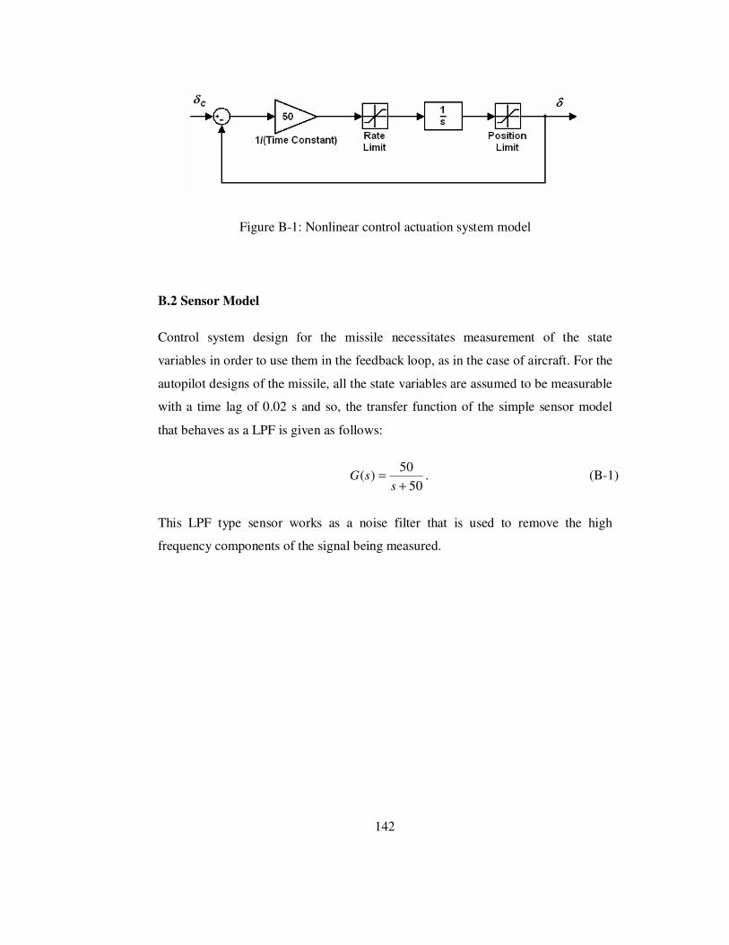
142

Figure B-1: Nonlinear control actuation system model

B.2 Sensor Model

Control system design for the missile necessitates measurement of the state

variables in order to use them in the feedback loop, as in the case of aircraft. For the

autopilot designs of the missile, all the state variables are assumed to be measurable

with a time lag of 0.02 s and so, the transfer function of the simple sensor model

that behaves as a LPF is given as follows:

50

50)(

+=

ssG . (B-1)

This LPF type sensor works as a noise filter that is used to remove the high

frequency components of the signal being measured.

a rule based missile evasion method for fighter aircrafts...

Documents