A Scalable Pattern Mining Approach to Web Graph Compression with Communities

Greg Buehrer and Kumar ChellapillaMicrosoft Live Labs

Motivation

Who links to me?How many hops is it from me to Kevin Bacon?What is the growth/impact of social network X?Are these web pages part of a link farm?

+ =>

Web Graph Compression• Goal: Reduce the memory footprint of the graph

• Existing Approaches [WWW04, DCC02, SHS]– Sort by URL to improve similarity between near nodes– Encode Id lists using a reference to a list in a near node, say within

5 nodes, called REFERENCE– Sort outlinks to minimize gap, code gap instead of Id, using

Huffman coding (or a similar flat code) – called GAP– Zeta Codes – Flat codes to code the gap (no lookup table required)

designed for power law distributionsNode Outlinks

1 2,10,12,14,18

2 5,10,12,14,18

Node Outlinks

1 2,10,12,14,18

2 (-1) +5,-2

Node Outlinks

1 8,2,2,2,4

2 (-1) +5,-2

Our ApproachMine for Dense Bipartite Graphs

20 Links [CN99, KDD00]

Virtual Node Miner

Virtual Node

9 Links (20/9) = 2.2x compression

Finding Bipartite Graphs

• Cast adjacency list as a transactional data set• Use pattern mining to find frequent itemsets

• Use an approximate mining strategy

Cust 1: milk bread cerealCust 2: milk bread eggs sugarCust 3: milk bread butterCust 4: eggs sugar

Node 1 Outlinks: 12,13,14,17Node 2 Outlinks: 12,13,14,19Node 3 Outlinks: 12,13,14,33Node 4 Outlinks: 3,4,12,13,14

=>

Webgraph Compression via Probabilistic Itemset Mining

• Perform mining in several steps1. Cluster/group similar nodes together using min-

wise hashing2. Finds patterns in the correlated group3. Create virtual nodes4. Substitute VN into graph5. Iterate

Find Patterns

Remove Patterns

Add Virtual Node

Cluster

Step 1 – Clustering

A. Use K min hashes to reduce each outlink list from variable length to length K, obtaining an n*K matrix

Id 1 2 3 4 K

1 hashA hashF hashW hashC hashB

2 hashF hashR hashA hashA hashB

3 hashA hashE hashA hashF hashC

n hashG hashR hashE hashG hashG

Clustering (cont)

B. Sort the matrix

Id 1 2 3 4 K

1 hashA hashF hashW hashC hashB

2 hashF hashR hashA hashA hashB

3 hashA hashE hashA hashF hashC

n hashG hashR hashE hashG hashG

Id 1 2 3 4 K

3 hashA hashE hashA hashF hashC

1 hashA hashF hashW hashC hashB

2 hashF hashR hashA hashA hashB

n hashG hashR hashE hashG hashG

Clustering (cont)3. Traverse the columns lexicographically,

grouping nodes with the same hash valueIf we reach K or have a small set, mine it

Id 1 2 3 4 K

3 hashA hashE hashA hashF hashC

1 hashA hashE hashA hashC hashB

2 hashA hashE hashW hashA hashB

n hashA hashR hashE hashG hashG

Step 2 - Mining1. Scan all node outlinks and record a histogram

of outlink ID frequenciesNode Id Outlinks

23 6,10,5,12,15, 1,2,3

102 1,2,3,20

55 2,3, 10,12,1,5,6,15

204 1,7,8,9,3

13 1,2,3,8

64 1,2,3,5,6,10,12,15

43 1,2,5,10,22,31,8,23,36,6

431 1,2,5,10,21,31,67,8,23,36,6

Id 1 2 3 5 6 10 8 12 15 23 31 36 7 9 20 21 22 67

Count 8 7 6 5 5 5 4 3 3 2 2 2 1 1 1 1 1 1

Node Id Outlinks

23 6,10,5,12,15, 1,2,3

102 1,2,3,20

55 2,3,1,5

204 1,7,8,9,3

13 1,2,3,8

64 1,2,3,5,6,10,12,15

43 1,2,5,10,22,31,8,23,36,6

431 1,2,5,10,21,31,67,8,23,36,6

Mining (cont)

2. Reorder each node’s outlink list based on the histogram (delete those with count=1)

Id 1 2 3 5 6 10 8 12 15 23 31 36 7 9 20 21 22 67

Count 8 7 6 5 5 5 4 3 3 2 2 2 1 1 1 1 1 1

Node Id Outlinks

23 1,2,3,5,6,10, 12,15

102 1,2,3

55 1,2,3,5,6,10,12,15

204 1,3,8

13 1,2,3,8

64 1,2,3,5,6,10,12,15

43 1,2,5,6,10,8,23,31,36

431 1,2,5,6,10,8,23,31,36

Mining (cont)

Node Id Outlinks

23 1,2,3,5,6,10, 12,15

102 1,2,3

55 1,2,3,5,6,10,12,15

204 1,3,8

13 1,2,3,8

64 1,2,3,5,6,10,12,15

43 1,2,5,6,10,8,23,31,36

431 1,2,5,6,10,8,23,31,36

3: {204}

8: {13}

23: {43,431}

31: {43,431}

36: {43,431}

10: {43,431}

8: {43,431}

8: {204}

1: {23}

2: {23}

3: {23}

5: {23}

6: {23}

10: {23}

12: {23}

15: {23}

1: {23,102}

2: {23,102}

3: {23,102}

5: {23}

15: {23,55,64}

12: {23,55,64}

3: {13,23,55,64,102}

5: {23,55,64}

1: {13,23,43,55,64,102,204,431}

2: {13,23,43,55,64,102,431}

3. Build a trie of the node outlink lists

6: {23,55,64}

10: {23,55,64}

5: {43,431}

6: {43,431}

Mining (cont)

4. Walk the trie and add candidate nodes to a list$ = (L-1)*(F-1)

|P| Node List $

9 43,431 8

|P| Node List $

9 43,431 8

3 13,23,43,55,64,102,431 8

|P| Node List $

9 43,431 8

3 13,23,43,55,64,102,431 6

8 23,55,64 14

3: {204}

8: {13}

23: {43,431}

31: {43,431}

36: {43,431}

10: {43,431}

8: {43,431}

8: {204}

1: {23}

2: {23}

3: {23}

5: {23}

6: {23}

10: {23}

12: {23}

15: {23}

1: {23,102}

2: {23,102}

3: {23,102}

5: {23}

15: {23,55,64}

12: {23,55,64}

3: {13,23,55,64,102}

5: {23,55,64}

1: {13,23,43,55,64,102,204,431}

2: {13,23,43,55,64,102,431}

6: {23,55,64}

10: {23,55,64}

5: {43,431}

6: {43,431}

|P| Node List $

9 43,431 8

2 13,23,43,55,64,102,431 6

8 23,55,64 14

3 13,23,55,64,102 8

Mining Stage (cont)

5. Sort the list based on their $– Including a Virtual Node for a pattern may rule out

another pattern

|P| Node List $

9 43,431 8

8 23,55,64 14

3 13,23,55,64,102 8

2 13,23,43,55,64,102,431 6

|P| Node List $

8 23,55,64 14

9 43,431 8

3 13,23,55,64,102 8

2 13,23,43,55,64,102,431 6

Node Id Outlinks

23 6,10,5,12,15, 1,2,3

102 1,2,3,20

55 2,3, 10,12,1,5,6,15

204 1,7,8,9,3

13 1,2,3,8

64 1,2,3,5,6,10,12,15

43 1,2,5,10,22,31,8,23,36,6

431 1,2,5,10,21,31,67,8,23,36,6

Mining (cont)6. Remove the top item in

the list and make a virtual node of it (replacing outlink IDs along the way)

|P| Node List $

8 23,55,64 14

9 43,431 8

3 13,23,55,64,102 8

2 13,23,43,55,64,102,431 6

Node Id Outlinks

23 V1

102 V3,20

55 V1

204 1,7,8,9,3

13 V3,8

64 V1

43 V2,22

431 V2,21,67

V1 1,2,5,6,10,8,23,31,36

V2 1,2

V3 1,2,3,5,6,10,12,15

Empirical Evaluation• Goal: Evaluate along 3 axes

– Compression, Scalability, Patterns Discovered– Implementation in C++– Windows Server 2003, 16GB RAM, 2.8GHz core

• Datasets from WebGraph data repository

Compression Afforded by VNodes

Webbase2001 is old and only has 8

edges/node

Total Compression

Compression Comparison

Bits per edge for Virtual Node Miner and WebGraph

Scalability

Virtual Node Properties

Communities are far apart

Reference schemes typically

have a small window size

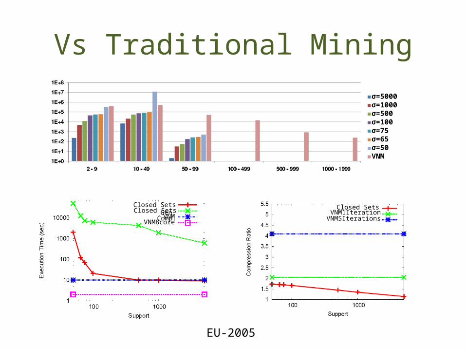
Vs Traditional Mining

σ=5000σ=1000σ=500σ=100σ=75σ=65σ=50VNM

VNM8core

Closed Sets Gen.Closed Sets Comp.

VNMVNM1Iteration

Closed Sets

VNM5Iterations

EU-2005

Take Home Message

• Web Graph Compression Contribution– Supports any URL ordering, any labeling– Supports any encoding scheme– Seeds for community discovery– High compression ratio– Scales well– Can be extended

• Data Mining – Log-linear itemset miner– Interesting data sets for pattern mining

Ongoing Work

• Computations on the compressed graph

• Ease of importing/updating data

• Compression for the full graph

Thanks!

[JCSS98] A. Broder, M. Charikar, A. Frieze, M. Mitzenmache. Min-wise Independent Permutations. In Journal of Computer and System Sciences, 1998.

[CN99] R. Kumar, P. Raghavan, S. Rajagopalan and A. Tomkins. Trawling the Web for emerging cyber-communities. In CN 1999.

[KDD00] G. Flake, S. Lawrence and C. Giles. Efficient identification of web communities. In KDD 2000.

[SIG00] J. Han, J. Pei and Y. Yin. Mining frequent patterns without candidate generation. In SIGMOD 2000.

[DCC02] K. Randall, R. Stata, R. Wickremesinghe and J. Wiener. The Link database: Fast access to graphs of the web. In DCC 2002.

[WWW04] P. Boldi and S. Vigna. The webgraph framework i: Compression Techniques. In WWW 2004.

[VLDB05] D. Gibson, R. Kumar and A. Tomkins. Discovering large dense subgraphs in massive graphs. In VLDB 2005.

External References

End of Talk

Extra slides for question support

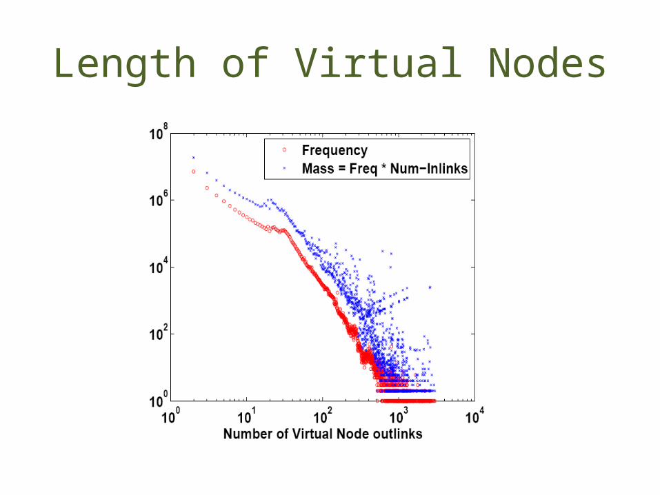
Length of Virtual Nodes

Compression as a Function of Pattern Length

Empirical EvaluationScalability and Execution Time

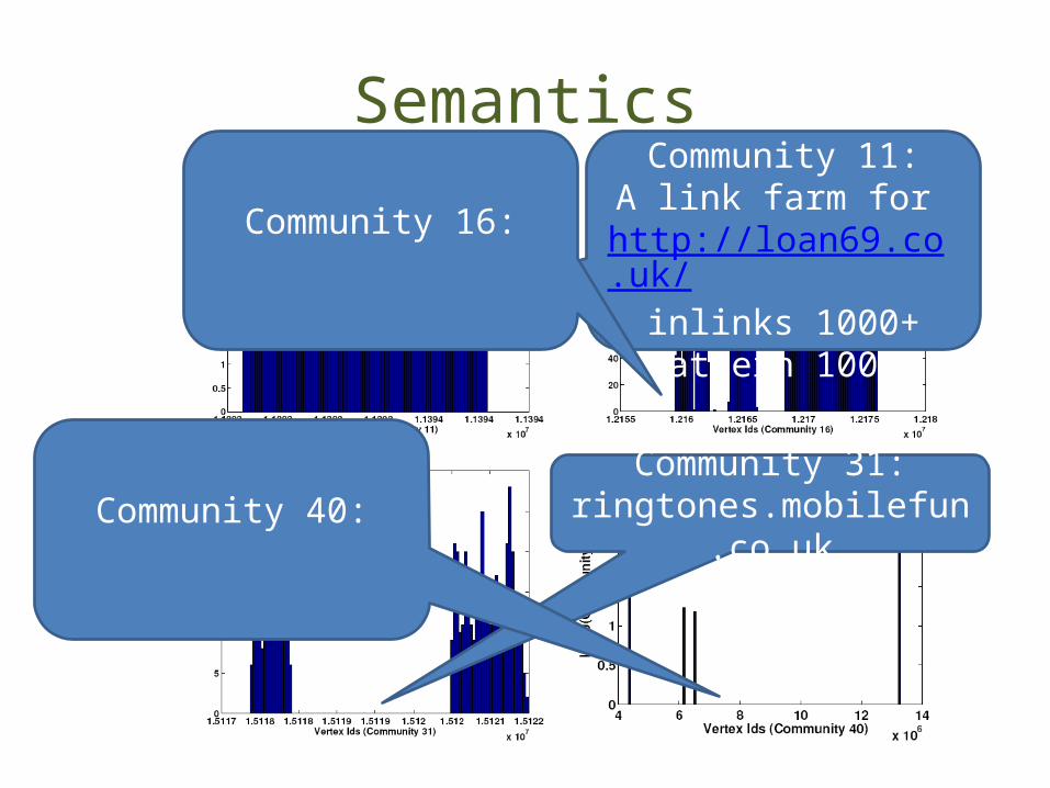
SemanticsCommunity 11:A link farm for

http://loan69.co.uk/inlinks 1000+pattern 1000+

Community 31:ringtones.mobilefun.co.uk

Community 16:

Community 40:

Optimality

• What if we were given every itemset and its frequency for free?

Optimality is intractable

An approximate solution may prove useful

1,2,4,5,9,10,12,13,14,18,23,34

Existing Itemset Mining Algorithms• Existing solutions have worst case exponential

runtimes [FIMI03]– Our use case is worst case (support=2)– Even streaming algorithms have worst case

exponential runtime complexities• Other patterns besides itemsets, such as

closed sets, maximal sets, and top-K sets also have exponential runtimes

Compression Components

Huffman coding degrades as VN compression increases